On Ad Hoc Communication in Industrial Environments


1
SEW-EURODRIVE GmbH & Co. KG, 76646 Bruchsal, Germany
2
Bochum University of Applied Sciences, Campus Velbert/Heiligenhaus, 42579 Heiligenhaus, Germany
*
Author to whom correspondence should be addressed.
Appl. Sci. 2020, 10(24), 9126; https://0-doi-org.brum.beds.ac.uk/10.3390/app10249126
Submission received: 20 November 2020
/
Revised: 11 December 2020
/
Accepted: 14 December 2020
/
Published: 21 December 2020
(This article belongs to the Special Issue Industry 4.0 Based Smart Manufacturing Systems)
Abstract
:Wireless communication is becoming vital in the industrial environment. New communication technologies, including ad hoc communication, are researched for this application. A thorough understanding regarding the connection characteristics of industrial networks could benefit this trend. In this work it was possible to record the time-variant network topology of such a network utilizing a novel method. Using this method and the generated recordings, novel insights into the behavior of industrial ad hoc networks are presented. The recorded time-variant topology, the tools and method of acquisition, and tools for processing and examination are published. This enables researchers and engineers to check their communication technologies in terms of applicability to the industrial use case and record more network topologies in a wide variety of wireless networking scenarios.
1. Introduction
Trends like Industry 4.0 are shaping the factory of the future. Flexibility and mobility are central requirements for future production facilities. Wireless communication plays a central part in enabling mobility and facilitating flexibility [1]. Automated guided vehicles (AGVs) for example, depend on wireless communication systems. Researchers are investigating the possibility of utilizing ad hoc communication (e.g., Mesh [2] or Delay Tolerant Networks (DTNs) [3]) for communication in AGVs. The research and implementation of wireless and ad hoc networks, in particular, would benefit from a thorough understanding of the wireless channel in industrial environments or the ability to simulate this use case. Additionally, further practical research is needed [4].
Research regarding wireless communication in industrial environments is challenging due to the limited accessibility of industrial facilities; thus, data from such facilities are sparse. This research aims to ease this challenge by publishing a data-set from a running production facility, and this enables researchers to test custom routing algorithms and networking strategies for ad hoc networks in an industrial scenario without accessing a production facility. Additionally, the tools for the creation, examination, and usage of this data-set are provided. The utilized method simplifies the scenario by abstracting the physical layer of the network and focusing on the connection-oriented aspects of communication. This work proposes a new method to record time-variant topologies of wireless networks and emphasizes its advantages over existing methods. The topologies of a mobile wireless network from a running production facility are recorded and published. These data enable researchers and engineers to test and verify networking strategies and routing algorithms. The connection-oriented topology characteristics are examined and compared to non-industrial and static wireless networks. Based on these comparisons, recommendations for the design of industrial ad hoc networks are given.
An encounter is a continuous time frame in which a transmitter can send data to a receiver and is the basic building block of a wireless network topology. A nodal encounter pattern (NEP) is a recording of the encounters in a specific scenario using a specific communication technology. The NEP denotes the time variant topology of the network and abstracts the physical layer of the communication interface. Properties of the NEP can therefore be used to determine connection characteristics of the used communication technologies in an examined scenario. This work contains a new method for recording and analyzing NEPs that were recorded in a running production facility. The NEPs are additionally published so the research community can use them for further analysis and as a basis for the simulation of wireless industrial networks. Although the NEPs recorded in this work are limited to the examined combination of the factory environment and communication technology, the proposed methods are applicable to a wide variety of applications and use cases. In terms of communication technology, the proposed method is limited to technologies that enable wireless broadcasting.
Utilizing NEPs to denote the time-variant topology of an industrial ad hoc network is novel and enables many new use cases. A researcher can, for example, use the published NEP to test a newly developed routing algorithm in regards to its applicability to an industrial use case when utilizing an IEEE802.11 interface. In another example, a research engineer can utilize the provided tools and record an NEP in a different environment, analyze the NEP, and select a communication technology on the basis of his observations.
The following research questions are answered by this work: How can the time-variant topology of a complex network be observed? What are the topology characteristics of an industrial ad hoc network? Additional topics regard the method of observing the topology, the applicability of different routing strategies to the industrial use case, and the ability to emulate a complex network without simulating it in detail.
The contribution of this work is four-fold:
- The applicability of an existing acquisition method for time-variant network topologies to the industrial use case is analyzed, and the method is found to not be applicable.
- A new method in the form of a custom protocol for recording time-variant network topologies is described and published. This includes the tools and methods for processing the acquired the data.
- NEPs describing the time-variant network topology of mobile industrial ad hoc networks are recorded and published for use by other researchers in further examinations and industrial ad hoc network simulations.
- The acquired NEPs are analyzed. Connection characteristics are extracted from these NEPs, and recommendations for suitable ad hoc networking solutions are given.
Wireless communication in the industrial context and related nodal encounter patterns are surveyed in Section 2. In Section 3 two different methods for NEP acquisition are compared in terms of their ability to represent the true network characteristics. Additionally, metrics are introduced, which characterize a wireless network and can be extracted from a NEP. Section 4 introduces the proposed and utilized tracing protocol and the process of encounter pattern generation from the recordings. The performed measurements and examined network characteristics are described in Section 5. Afterwards, Section 6 concludes this work with a discussion on methods and presented observations.
2. Related Work
Wireless communication is not new in the industrial context, but it has continuously gained importance [5,6]. The industrial environment is particularly challenging for the application of wireless communication technologies [7]. On the one hand, high requirements in terms of latency, throughput, and especially reliability are applied [8,9]. On the other hand, dynamic environments including fading, mobility in the transmitter and receiver, and the permanent presence of interference degrade the performance of wireless communication technologies. Fellan et al. and Zhang et al. [10,11] analyzed these challenging requirements for the communication systems of mobile robots in the Industry 4.0 context. The requirements for different industrial use cases were compared and the applicability of several communication technologies examined.
Relevant communication technologies for the industrial AGV use case include LTE [12], 5G [1,13], WiFi [11,14], ZigBee [11], and specialized solutions like visible light communication (VLC) [15] and radar [16]. These technologies have different advantages and strengths and must be chosen based on the application specific requirements. References [5,10,11,16] compare these strengths to the requirements of emerging industrial trends. This high variability in underlying communication technology makes it necessary to develop methods that do not depend on specific technologies.
References [17,18,19,20,21,22,23,24] performed measurements in different industrial environments and provide valuable insight on the expected channel characteristics at different frequencies. The observed variability of the link over time is a strong indicator for the dynamic nature of the propagation properties within an industrial environment. The measurements were executed with static transmitter and receivers at different positions. Spatial variability is an important factor in scenarios, where the transmitter and/or receiver are mobile [14]. Reference [25] illustrates the lack of measurements in industrial applications. No previous work has specifically characterized the peer-to-peer communication channels in a mobile industrial network. Additionally, the previously published measurements of wireless channel propagation characteristics lack abstraction towards available connections that the utilized method provides. Thus, this works provides a complementary approach to existing work.
Ad hoc communication technologies are an emerging trend in the use case of factory automation and industry in general. Wireless sensor networks (WSN) are possibly the best established use case for this technology [26,27]. These sensor networks are utilized to monitor machines, environmental conditions, and more. Software-Defined WSN (SDWSN) are a particular variant of these networks, surveyed by [4].
Mobile Ad hoc NETworks (MANET) are not yet present in many industrial facilities. However, they are being investigated by researchers in the context of mobile robots (e.g., AGVs) [2]. In this use case, MANETs and other other ad hoc technologies, like delay tolerant networks (DTNs) [3], offer enhanced flexibility, reliability, and independence from network infrastructure. The applicability of existing communication and routing solutions to an industrial MANET have not been researched at this point in time. This work offers, in contrast to previous work, a non-simulation-based, routing-independent view on the mobile industrial peer-to-peer channel. It is therefore useful as a foundation for future research on ad hoc technologies in the industrial environment. In contrast to the presented methods, the observed connection characteristics depend on the chosen combination of examined environment and communication technologies.
NEPs have previously been used to examine mobile ad hoc networks [28]. Hsu et al. used NEPs to examine the properties and applicability of ad hoc data dissemination schemes to campus networks. They acquired NEPs using network traces [29,30] from the campus networks of several universities. These traces contain the complete communication within the examined infrastructure network, including the registration of mobile devices at certain access points. With the assumption that two nodes registered at the same access point can also directly communicate with each other, NEPs are extracted from the network traces [31]. The presented work, in contrast, utilizes a novel protocol to directly record NEPs. This enables a more precise observation of the network without assumptions about the connectivity of clients.
No previous work has analyzed the ad hoc communication channel of mobile clients in an industrial environment. With ongoing trends like Industry 4.0, the importance of mobile clients and wireless communication will increase. Therefore, this investigation is highly relevant. Additionally, this work uses the established tool NEP to examine the ad hoc channel and proposes and publishes a new method to record these NEPs, which can be applied with other communication technologies in industrial scenarios, but also in non-industrial applications.
3. Comparing Methods for the Extraction of NEPs
It is hypothesized that the necessary base assumption for the NEP extraction from network traces is not applicable to the industrial scenario. In this section differences between the indirect generation of NEPs by means of network traces and the direct recording of NEPs by means of a custom protocol are shown. Two primary metrics are examined.
The average number of simultaneous encountered per node and the average duration of these encounters are examined. Both metrics can be directly calculated from a NEP. Both metrics are important when analyzing the characteristics of the ad hoc communication channels. The first is an indicator for the number of reachable destinations from any node, while the second indicates the duration for which these destinations are reachable.
The first NEP acquisition method is the acquisition by means of a custom protocol, further denoted as trace protocol. The protocol is described in Section 4. The second is the acquisition by means of network traces [28]. This second method is based on the assumption that any two nodes encounter each other if they are registered at the same access point. Both approaches have different strengths and weaknesses.
In this section the fundamental behavioral differences of encounters acquired by both methods are observed. The goal is to analyze the behavior of the average number of simultaneous encounters in regards to the number of nodes N and number of access points . Additionally, the average encounter duration in regards to the communication range r of the nodes and their speed v is analyzed. The communication range r results in a node coverage area .
In the following subsections the behavior of the average number of simultaneous encountered per node and the average duration of these encounters are explored. describes the type of examined acquisition method. is the recording of encounters by means of the tracing protocol, and is the acquisition by means of network traces. Models are proposed to emulate the behavior of the different metrics, when observed by the different methods. The goal of these models is to predict the network performance, as best as possible, given the impact of certain network parameters on the network behavior.
3.1. Average Number of Simultaneous Encounters per Node
With the assumption of equally distributed, randomly placed access points and randomly moving nodes on area A, can be determined for both acquisition methods. For the observation by trace protocol, the number of nodes that a specific node might encounter is calculated. It is expected that the other nodes are randomly distributed on A. The number of simultaneously encountered nodes is therefore expected to be the fraction of that are present in . It follows that
For the acquisition by means of network traces , two different cases must be considered. The first case is that the area A is not completely covered by access points. This case is defined by . This means that the combined covered area by all access point is smaller than A. Overlap of access point communication ranges is rare, due to the assumed equal distribution of access points. If the area is not completely covered, the average number of simultaneous encounters is equal to the average number of nodes, within range of an access point minus the source node () times the probability, to be within the range of an access point (). When assuming complete coverage of the area this probability is 1. Once the area is completely covered, the covered area per access point decreases because the nodes will tend to register at the closest access point. In reality, the chosen access point depends on the applied roaming scheme; most are based on received signal strength. This decline can be formalized with , where . It simplifies to
The model for the acquisition via trace protocol is therefore equal to the model for the acquisition via network trace only for the case and a perfect 1:1 coverage of the application area by the access points. Later results show differences even in this case.
3.2. Average Duration of Encounters
The average duration of encounters is mostly dependent on the mobility of the nodes. Hsu et al. [28] assumed nodes stayed within the range of an access point for a prolonged duration. This assumption minimizes the influence of mobility on the encounter pattern, which is a valid assumption for the examined network traces. In the examined campus networks, students listen to lectures or visit libraries and similar locations for a duration of h. This assumption, however, is not transferable to the examined use case of AGVs in an industrial environment; therefore, the effect of mobility on the two observation methods must be considered.
The proposed models reduce the dependencies of the encounter duration of two nodes to the speed v of the nodes and the communication range r. On average, a moving node passes the static communication range of an access point along a path of length (see Figure A2) and therefore for a time of . This average only accounts for a node passing an AP range. If the destination of the node is within the AP range, the average traveled distance within communication range (average destination is at the AP position; distance to reach the AP and subsequently leave range is ) changes to . It is assumed that ; therefore, this special case is subsequently not considered. An encounter between any two nodes persists as long as both are in range of the access point. At the point in time at which any node enters the range, every other node that already is connected to the AP will leave the range after . Therefore, the average encounter duration of two nodes can be reduced to :
Analogous to the model of , the case of complete coverage has to be considered when calculating the duration. This is done with the scaled access point communication radius .
Determining the encounter duration of two mobile nodes is challenging. Therefore, an approximate for the average encounter duration was determined via a fit to data from extensive simulation:
For typical values of A the best fit was generated with . Both models are highly simplified. For the model of NEP acquisition via network trace, a dependence on can be observed. The duration of encounters in a real ad hoc network, however, does not depend on this parameter.
3.3. Numerical Comparison
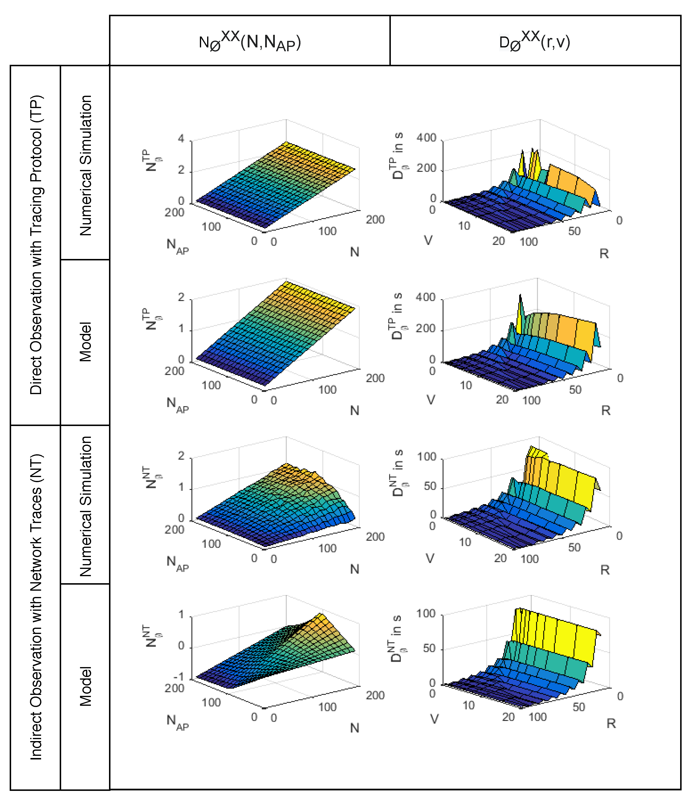
The proposed models for , , , and were compared to a numerical simulation of an ad hoc network. In this simulation, the nodes use the Random WayPoint Model [32] to move within the confined area. The results of the proposed models and the numerical simulation are presented in Appendix A.
In Appendix A it can be seen that the numerical simulation behaved similarly to the proposed models. This validates that the proposed models are able to estimate the network performance and behavior without simulating the complete network.The plots of the performance predicted by observations from tracing protocol and from network traces, however, are highly dissimilar; this suggests that the assumptions of the NEP generation from network traces are not applicable.
The numeric simulation confirms the behavior expected from the presented models. Models and simulations show the same behavior in regards to parameters and similar network performance. Figure A1 also shows the differences of the two methodologies and . The two acquisition types showed clear behavioral differences, which are examined in detail in the following subsection. Only for specific configurations of N, , v, and r can similar results in terms of N∅ and D∅ be obtained from both acquisition methods. All these observations were done under assumptions of random node mobility and random access point placement. More complex distributions of nodes and APs will lead to even more complex relations between all of these parameters and metrics, and even more pronounced differences between both acquisition methods.
3.4. Behavioral Differences
The average number of simultaneous encounters and the average encounter duration are two metrics that change their behavior in regard to the applied acquisition method. Direct acquisition by means of a tracing protocol enables the more precise examination of a network. Using this method, both metrics behave as expected. The number of encounters increases linearly with the number of mobile nodes. The duration of the encounters is constant when the communication range and node speed are not changed. Both extensive simulation and the proposed model confirm this intuitively expected behavior.
The indirect acquisition by means of network traces shows a different behavior. The number of access points is important when observing the behavior with this method. The duration of encounters is lower than expected, and further declines when the density of access points is increased. A higher density of access points is beneficial when observing the number of encounters. The best fit to the direct observation is at the point of full coverage (). At higher access point density the number of encounters decreases. In both metrics the decrease is caused by the higher probability for overlapping of the communication ranges of the access points.
The direct acquisition by means of a tracing protocol is therefore recommended. Even if the number of access points is known, a correction of these metrics is hardly possible due to the complex spatial distribution of nodes and access points in real networks [33].
Using a tracing protocol for the acquisition of NEPs also has the advantage that encounters can be directional. This means that node A can send data to node B, while node B cannot send data to node A. This directionality in encounters can not be extracted when a network trace is the basis of the NEP. However, this is of major importance when evaluating the applicability of certain routing protocols.
4. Tracing Protocol
NEPs describe encounters between nodes of a wireless network [28]. The patterns can be used two-fold. Firstly, they can be analyzed independently to determine specific network or channel characteristics, like bidirectionality, encounter duration, and more. Secondly, they can replace the mobility model, signal propagation model, and the lowest layers of the network model in a network simulation. A NEP has the advantage of being extracted from the examined environment; therefore, no complex validation of models is necessary.
The goal of this section is to introduce a protocol that can be executed on mobile nodes (e.g., AGVs in a production facility) and generate a NEP. The protocol and the required processing are described, and a simple implementation based on the Click-Router [34] is published [35]. The tracing protocol has the advantage that the real NEP can be directly recorded, but the protocol must be implemented and running on all observed nodes.
Protocol Description
The basic idea of the protocol is to use beacons to indicate the possibility of data exchange between a transmitter T and a receiver R. A number of nodes is placed in the examined environment. All nodes send beacons with a certain frequency . If any beacon is received by any receiver, it is logged to a log file. After the recording is completed, the log files of all nodes are processed, and a NEP is created.
The nodes are all identical in function. The protocol defines a time step . This is the time resolution of the resulting NEP. A smaller leads to a higher resolution in the NEP and to a higher bandwidth usage by the protocol. For the channel to be non-changing within , must be chosen to be smaller than the coherence time of the communication channel. In the case of wireless communication at GHz and a node speed of m/s, the time resolution should be chosen to be smaller than 25 ms. An address is assigned to every node, and a counter is incremented every time the node sends a beacon. Beacons are send every . The beacon contains the address of the transmitter and the current index of the transmitter .
This beacon is send by the wireless interface (e.g., WiFi IEEE802.11 b/g/n) of the node. Any receiver () logs this beacon as an encounter tuple, with r being the receiver and s the transmitter. All recorded encounter tuples can be concatenated to form an encounter recording , which is a set of encounter tuples recorded by node R.
Any entry in the recording describes the start or persistence of an encounter of the nodes T and R. It is important to note that these encounters are directional. The entry only indicates a connection from T to R, not vice versa. A second entry must indicate the reverse encounter.
With the indices can be converted to time values. All connections have two time values. This is necessary to compensate for time offset and drift between the internal clocks of the nodes. The encounter recordings of all nodes can be concatenated to form . The clock offset is compensated by choosing a reference node , and for every other node an offset has to be determined. For every non-reference node n a time pair is extracted from , where is the record time of the receiver, while is the send time recorded at the transmitter. The discrete offset function can be made continuous by assuming, for example, no or linear drift between the clocks of node and n. The offset is subsequently compensated by the following conversion:
An offset compensated encounter list L is the result, when applying this offset to all entries.
The NEP is subsequently a function of the transmitter T, the receiver R, and the time t. It is defined as
For computational purposes this function is represented as a 3d matrix of the dimension , with N being the number of nodes that were used for the recording, and the last dimension offers one entry per time step for the complete measurement time t.
5. Examination of the Industrial Ad Hoc Channels
Measurements with the proposed tracing protocol were performed in different environments and under varying conditions. The goal of the measurements and the analysis is to characterize the industrial environment in terms of effects on ad hoc communication channels. Knowing the characteristics of a communication channel allows for a more effective selection and configuration of applied routing solutions. The networks examined by Hsu et al. [28] are fundamentally different from the network examined in this work. The number of clients, the kind of mobility, and the environment are the most obvious differences. Different metrics for these network characterizations are therefore applied in this work.
Bai et al. [36] showed that after sufficient time all nodes of a network encounter each other if they move randomly on the same area. AGVs do not move randomly, but for the examined small networks the same behavior was observed. It is expected that, in bigger AGV systems, it may not be true all AGVs encounter all other AGVs. Certain AGVs could, for example, exclusively transport goods within specified disjoint areas.
The industrial environment where the measurements took place involves electric drives and gear production that adhere to Industry 4.0 paradigms, although it is a brown-field factory. Thus, a typical industrial environment by means of the amount of mobility and conductive material is present. The AGVs that were equipped with the measurement equipment facilitate intra-logistic processes of half-finished and finished products and drive up to m/s. They cover an area of ≈25,000 m.
5.1. Performed Tests
In order to evaluate the channel characteristics of industrial ad hoc channels, tests in different environments and with different setups were conducted. The goal is to differentiate between the influence of environment and mobility on ad hoc communication and how to extract this information from the NEPs.
A reference test was performed to check the general functionality of the protocol and to deliver a reference for the examined network characteristics. It was performed in an office environment with static nodes.
A static industry test describes the measurement with nodes in an industrial environment. In this test all nodes collectively moved in an industrial environment; hence, they did not experience any relative movement and therefore moved as one group. The goal of this test is to characterize the effect of interference on the industry, while mitigating the effects of mobility and variable signal propagation. The absolute movement of the node group enabled the observation of the spatial variation in the interference.
Lastly a mobile industry test was conducted by utilizing AGVs in an accessible production facility to implement mobility. The nodes were mounted on the AGVs in an unobstructed way. Therefore, two signal attenuation effects influenced the existence of encounters in the resulting NEP. Firstly, large scale fading causes path loss between transmitter and receiver due to the distance between them. Secondly, small-scale fading caused by reflection, refraction, and scattering can be caused by obstacles on the primary propagation path.
The tests are characterized by a number of varying parameters. When comparing the presented results of the measurements, variations in these parameters have to be taken into account. Table 1 compiles and describes the different parameters and their values for the performed experiments.
Some parameters are restricted by external requirements. The send period of the trace protocol, for example, had to be adjusted, as a minimal bandwidth impact of the measurement was required. Table 1 compares the measurement parameters of the three measurements.
5.2. Network Connectedness
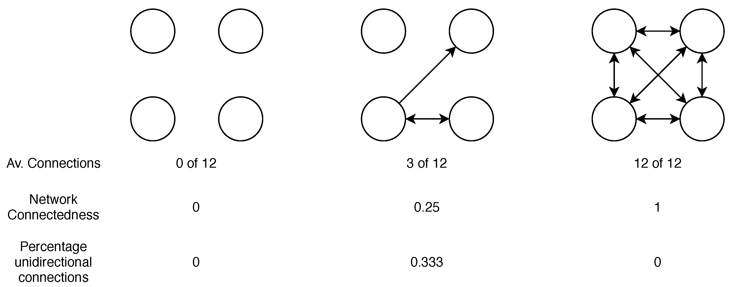
The network connectedness is the average percentile of neighboring nodes (encountered nodes with which direct data exchange is possible) [33]. A connection can be established if an encounter is registered. It is assumed that two nodes could communicate for the time of 1 dt after an encounter was registered. Within a network of n nodes, connections are simultaneously possible for any node. Hence, nodes cannot connect to themselves. The network connectedness of the network at time t is then defined as
where C is the NEP, as described in Section 4, and i and j iterate over N nodes (transmitter and receiver) in the examined network. When de-normalized and averaged over the time of the recording, the network connectedness is equal to the previously used metric . Figure 1 illustrates the meaning of different network connectedness values. A network connectedness describes a network where no nodes are connected. The network connectedness increases once connections are available. If all nodes can reach all other nodes the network connectedness reaches 1.
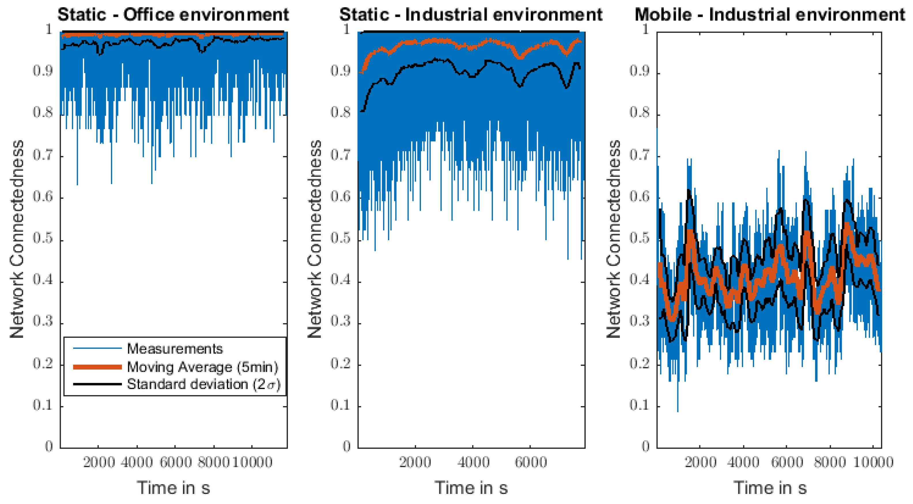
The network connectedness of the three examined measurement configurations are displayed in Figure 2. On average, the network in the reference measurement is fully connected. This means all nodes can communicate with all other nodes. Short-lived variations occur due to interference between the nodes and interference with other wireless communication systems within the same spectrum. The second measurement set shows slightly lower connectedness within the network. This indicates that the industrial environment might contain more sources for interference than the office environment. The variations in network connectedness indicate spatial correlation. The NEP of mobile nodes in the industrial environment exhibits the lowest network connectedness and even higher variations in connectedness as the static measurement in the industrial environment. In Figure 2 it can be seen that the effect of mobility is far more pronounced than the one of interference.
5.3. Directional Channel Probability
Consider a transmitter A sent a message to receiver B at time . In this work a channel is classified as unidirectional if a transmission at time from B was not received at A. If the transmission is received, the channel is classified as bidirectional. Possible reasons for unidirectional channels are changes in the propagation path within or interference with other communication networks. The office reference test shows that interference within the tracing protocol is unlikely.
Many common routing protocols (e.g., DSR [37], AODV [38]) expect bidirectional connections. Routing protocols can be enhanced to work in the presence of unidirectional channels at the cost of higher overhead [39]. The percentage of unidirectional connection is therefore highly relevant in the evaluation of the applicability of ad hoc routing protocols to the industrial environment. We assume that such protocols need at least about 200 ms for route search and establishment; therefore, the chosen s NEP time resolution is sufficient for the examined application.
NEPs that were extracted from the proposed trace protocol can be used to determine this probability of a channel being unidirectional. It is defined by Equation (9) using the same parameters as Equation (8).
Previously shown, Figure 1 illustrated examples for the percentage of channels that are unidirectional. In the central graph three connections exist. One of these connections has no reverse connection. Therefore, one-third of all connections are unidirectional.
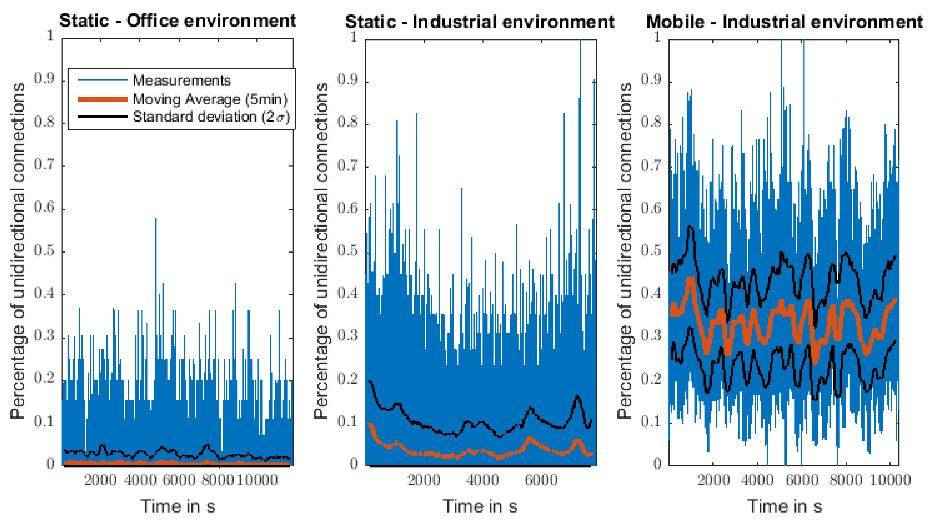
As seen in Figure 3, the percentage of unidirectional connections is much higher in mobile industrial scenarios than in the reference use case. In the static reference measurement, unidirectional connections are very rare and only of short duration. On average only % of all connections are unidirectional. In contrast, about % of all connections are unidirectional in the mobile industrial scenario. In the static industrial scenario, on average about % of all connections are unidirectional. The results therefore support the previous observations that node mobility has a higher impact on the wireless channel than the industrial environment. Overall, such channel characteristics have to be taken into account when selecting or designing a routing protocol for the industrial use case. Another important aspect for this task is the route lifetime.
5.4. Route Lifetime
The route lifetime describes how long a connection between two nodes persists before the ability to transmit data is lost. This is an important parameter in the analysis of applicability for certain network technologies. A low route lifetime would, for example, lead to more route failures and therefore more overhead in a MANET routing protocol. The average route lifetime is equivalent to the previously used parameter .
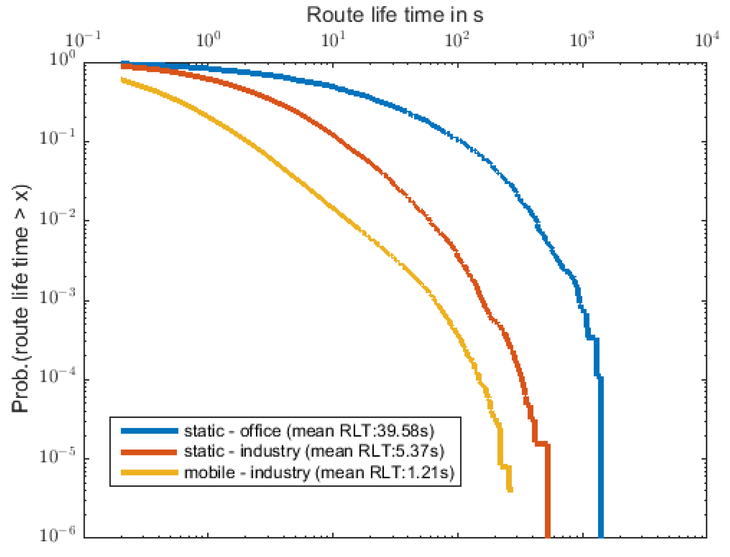
Figure 4 shows the probabilities for route lifetimes in the three scenarios. This metric also iterates the same trend as the previous: From static office scenario over static industrial scenario to mobile industrial scenario the route life time decreases. In the static office scenario an average route life time of about 39 s was observed. Interference between nodes or with other signal sources is rare. This route lifetime significantly decreases when the same setup is observed under industrial conditions. The route lifetime further decreases when observing mobile nodes. Two AGVs are within communication range for far longer than s (assuming a communication range m and an AGV speed m/s; an encounter duration of 20 s follows); therefore, the further decrease in route lifetime cannot be explained by the distance between the AGVs and their communication range. Rather, effects on the primary line-of-sight path or on secondary propagation paths might be the cause of the increased number of disconnections.
5.5. Effects of Multi-Hop Relaying
Mobile Ad hoc NETworks (MANETs) [2], Delay Tolerant Networks (DTNs) [3] and Wireless Sensor Networks (WSNs) [27] are emerging and developing trends in the industrial context. An ad hoc network’s major advantage over infrastructure networks (e.g., WiFi) is flexibility and redundancy. They are envisioned to mitigate the dependence on network infrastructure and enhance a combined wireless network structure.
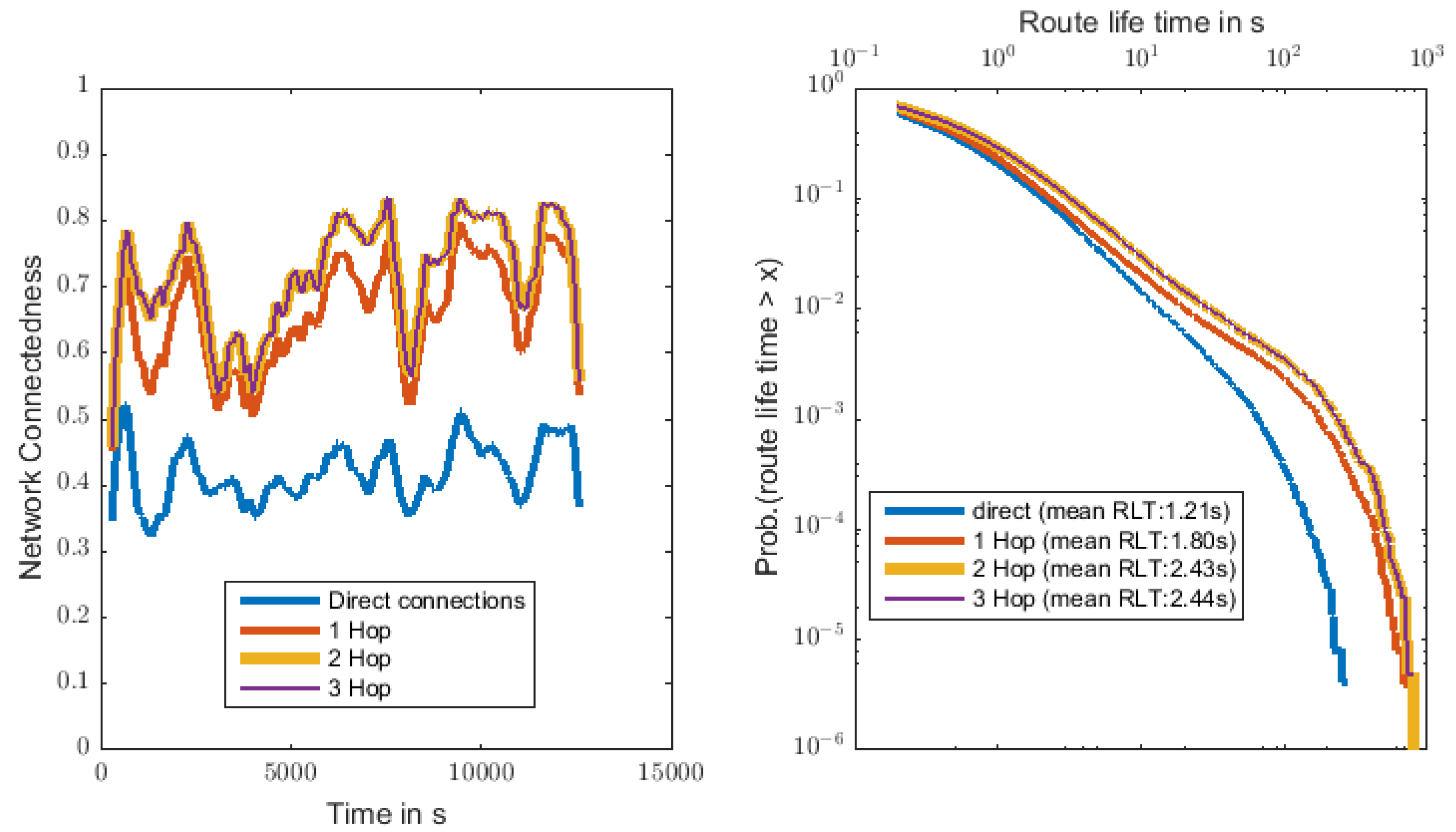
In this work the NEP is used to examine the advantage of redundant multi-hop links between mobile nodes in industrial environments. The previously examined route lifetime is the primary metric for evaluating the improvement. It is envisioned that the utilization of redundant links increases the route lifetime. Another expected improvement will be that multi-hop relaying enhances the network connectedness. In this examination only the mobile industrial measurements are used. Different network sizes, in terms of number of hops, are examined.
The relevant metrics regarding both expectations were examined and are presented in Figure 5. It can be confirmed that the utilization of multi-hop connections is beneficial in the mobile industrial context. Firstly, the network connectedness increases; therefore, more nodes can be reached by any other node. Secondly, the average route lifetime is positively affected. The number of available hops is highly relevant when examining these benefits. For the examinations it must be assumed that finding and establishing a route of length h (in hops) is possible within . As illustrated in Figure 5, the first hop is the most effective in increasing network connectedness and route lifetime. It is suspected that in AGV scenarios with more mobile nodes and/or on a bigger area, more hops would be effective in increasing the network connectedness. In the observed scenarios the first and second hops were most effective in enhancing the route lifetime, while only the first hop enhanced the number of reachable nodes.
6. Conclusions
This work examined the time-variant network topology of ad hoc communication under industrial conditions. Existing methods for the extraction of these topologies from network traces were examined. It is concluded that the direct observation of encounters with a novel custom protocol can more accurately represent the behavior of an ad hoc network compared to the work in [28]. The custom protocol was implemented, tested, and used in an industrial environment. The protocol is made available for researchers and engineers to analyze the behavior of other network applications. The time-variant topologies that were recorded are also made available. The examined production facility followed the principles of Industry 4.0. To the best of our knowledge, we are the first to provide comprehensive measurements that characterize ad hoc network behavior in this context. With these recordings, researchers and engineers (can for the first time) analyze, simulate, and test industry-specific communication solutions for the factory of the future. Additionally, the acquired topologies were analyzed in terms of general network behavior with the goal to give general recommendations for communication system design.
The ad hoc channels in an industrial environment present some challenging characteristics. The observations of network connectedness (sparse vs. fully meshed) suggest that interference impacts the channel availability in the industry. Mobility of the clients, however, has by far higher effects on the availability of channels between nodes. The analysis of the bidirectionality of the available channels suggests that many existing MANET protocols are not applicable to the shop floor. The high percentage of unidirectional connection (30% to 35%) highly impacts the search for routes and increases the resulting routing overhead. The network performance is further impacted by the low route lifetime. For the ad hoc channels between mobile clients in the industrial environment, an average route life time of s was observed. In regards to route lifetime, interference in the industrial environment has the higher impact factor, compared to the mobility. Lastly, the effects of multi-hop networks on the network connectedness and route lifetime were observed. Both benefit especially from the inclusion of the first and second relay/hop. This is an interesting observation when considering the availability of technologies like Side-Link for 5G. Even more hops have an even bigger effect, but the benefit decreases. The presented observations are currently limited to the wireless peer-to-peer channel of IEEE802.11 interfaces. However, the proposed methods are applicable to any other broadcast-enabled communication technology.
The presented results illustrate the benefits of industrial MANETs, as well as the challenges. In the future it is planned to acquire more NEPs from a rich set of industrial and other environments and a variety of wireless communication technologies. This data-set will benefit us in the design and testing of industrial MANETs and a unified communication framework for mobile robots in the industry. Additionally, the acquired NEPs shall be used to test different routing protocols, where the results will be validated by experimental MANET implementations in production facilities.
Author Contributions
Conceptualization, C.S. and M.S.; methodology, C.S.; software, C.S.; validation, C.S., M.S. and E.L.; formal analysis, C.S. and E.L.; investigation, E.L. and C.S.; resources, C.S.; data curation, C.S.; writing—original draft preparation, C.S. and E.L.; writing—review and editing, C.S., E.L. and M.S.; visualization, C.S.; supervision, M.S.; project administration, C.S. All authors have read and agreed to the published version of the manuscript.
Funding
This research received no external funding.
Conflicts of Interest
The authors declare no conflict of interest. The funders had no role in the design of the study; in the collection, analyses, or interpretation of data; in the writing of the manuscript, or in the decision to publish the results.
Appendix A. Simulation and Model Results
Results of numerical simulations are described and analyzed in Section 3.3.
Figure A1.
Comparison of the proposed model and numerical simulation.

Appendix B. Theorem of Circle Intersection Length
Theorem A1.
The chord length of a circle intersection depends on the radius r of the circle and the distance s of the chord to the center of the circle. With these two values α can be determined as . The length of the intersection is subsequently defined as . In the scenario of randomly driving nodes through the circle, it is assumed that s is equally distributed over . With this assumption the intersection length can be averaged over the distribution as follows:
Figure A2.
Line intersecting a circle.

References
- 5G ACIA. 5G for Connected Industries and Automation; Technical Report; ZVEI—German Electrical and Electronic Manufacturers: Frankfurt, Germany, 2018. [Google Scholar]
- Jarchlo, E.A.; Haxhibeqiri, J.; Moerman, I.; Hoebeke, J. To Mesh or not to Mesh: Flexible Wireless Indoor Communication among Mobile Robots in Industrial Environments. In Proceedings of the AdHoc-Now, Lille, France, 4–6 July 2016. [Google Scholar]
- Sauer, C.; Schmidt, M.; Sliskovic, M. Delay Tolerant Networks in Industrial Applications. In Proceedings of the IEEE ETFA, Zaragoza, Spain, 10–13 September 2019. [Google Scholar]
- Kobo, H.I.; Abu-Mahfouz, A.M.; Hancke, G.P. A Survey on Software-Defined Wireless Sensor Networks: Challenges and Design Requirements. IEEE Access 2017. [Google Scholar] [CrossRef]
- Wollschlaeger, M.; Sauter, T.; Jasperneite, J. The Future of Industrial Communication: Automation Networks in the Era of the Internet of Things and Industry 4.0. IEEE Ind. Electron. Mag. 2017. [Google Scholar] [CrossRef]
- Ericsson. The Industry Impact of 5G. Self-Published. 2018. Available online: https://files.vogel.de/vogelonline/files/9763.pdf (accessed on 18 December 2020).
- Lucas-Estañ, M.C.; Maestre, J.L.; Coll-Perales, B.; Gozalvez, J.; Lluvia, I. An Experimental Evaluation of Redundancy in Industrial Wireless Communications. In Proceedings of the 2018 IEEE 23rd International Conference on Emerging Technologies and Factory Automation (ETFA), Turin, Italy, 4–7 September 2018; Volume 1, pp. 1075–1078. [Google Scholar] [CrossRef]
- Chen, H.; Abbas, R.; Cheng, P.; Shirvanimoghaddam, M.; Hardjawana, W.; Bao, W.; Li, Y.; Vucetic, B. Ultra-Reliable Low Latency Cellular Networks: Use Cases, Challenges and Approaches. IEEE Commun. Mag. 2018, 56, 119–125. [Google Scholar] [CrossRef] [Green Version]
- 3GPP. TR22.804 Study on Communication for Automation in Vertical Domains (Release 16); Technical Report; 3GPP, Sophia Antipolis Cedex: Valbonne, France, 2018. [Google Scholar]
- Fellan, A.; Schellenberger, C.; Zimmermann, M.; Schotten, H.D. Enabling Communication Technologies for Automated Unmanned Vehicles in Industry 4.0. In Proceedings of the ICTC, Jeju, Korea, 17–19 October 2018. [Google Scholar]
- Zhang, M.; Yu, K. Wireless Communication Technologies in Automated Guided Vehicles: Survey and Analysis. In Proceedings of the IEEE IECON, Washington, DC, USA, 21–23 October 2018. [Google Scholar]
- Lyczkowski, E.; Munz, H.; Kiess, W.; Joshi, P. Performance of Private LTE on the Factory Floor during Production. In Proceedings of the IEEE ICC Workshop, Dublin, Ireland, 7–11 June 2020. [Google Scholar]
- Gidlund, M.; Lennvall, T.; Åkerberg, J. Will 5G become yet another Wireless Technology for Industrial Automation? In Proceedings of the IEEE ICIT, Toronto, ON, Canada, 22–25 March 2017. [Google Scholar] [CrossRef] [Green Version]
- Lucas-Estañ, M.; Maestre, J.; Coll-Perales, B.; Gozalvez, J.; Lluvia, I. An Experimental Evaluation of Redundancy in Industrial Wireless Communications. In Proceedings of the IEEE ETFA, Turin, Italy, 4–7 September 2018. [Google Scholar]
- Pathak, P.H.; Feng, X.; Hu, P.; Mohapatra, P. Visible Light Communication, Networking, and Sensing: A Survey, Potential and Challenges. IEEE Commun. Surv. Tutor. 2015, 17, 2047–2077. [Google Scholar] [CrossRef]
- Lyczkowski, E.; Wanjek, A.; Sauer, C. Wireless Communication in Industrial Applications. In Proceedings of the IEEE ETFA, Zaragoza, Spain, 10–13 September 2019. [Google Scholar]
- Willig, A.; Kubisch, M.; Hoene, C.; Wolisz, A. Measurements of a wireless link in an industrial environment using an IEEE 802.11-compliant physical layer. IEEE Trans. Ind. Electron. 2002, 49, 1265–1282. [Google Scholar] [CrossRef] [Green Version]
- Chrysikos, T.; Georgakopoulos, P.; Oikonomou, I.; Kotsopoulos, S.; Zevgolis, D. Channel Measurement and Characterization for a Complex Industrial and Office Topology at 2.4 GHz. In Proceedings of the SKIMA, Malabe, Sri Lanka, 6–8 December 2017. [Google Scholar] [CrossRef]
- Chrysikos, T.; Georgakopoulos, P.; Oikonomou, I.; Kotsopoulos, S. Measurement-based Characterization of the 3.5 GHz Channel for 5G-enabled IoT at Complex Industrial and Office Topologies. In Proceedings of the IEEE WTS, Phoenix, AZ, USA, 17–20 April 2018. [Google Scholar] [CrossRef]
- Adegoke, E.I.; Edwards, R.M.; Whittow, W.G.; Bindel, A. Characterizing the Indoor Industrial Channel at 3.5GHz for 5G. In Proceedings of the 2019 Wireless Days (WD), Manchester, UK, 24–26 April 2019; pp. 1–4. [Google Scholar] [CrossRef]
- Tanghe, E.; Joseph, W.; Verloock, L.; Martens, L.; Capoen, H.; Herwegen, K.V.; Vantomme, W. The industrial indoor channel: Large-scale and temporal fading at 900, 2400, and 5200 MHz. IEEE Trans. Wirel. Commun. 2008, 7, 2740–2751. [Google Scholar] [CrossRef]
- Ai, Y.; Cheffena, M.; Li, Q. Power delay profile analysis and modeling of industrial indoor channels. In Proceedings of the 2015 9th European Conference on Antennas and Propagation (EuCAP), Lisbon, Portugal, 13–17 April 2015; pp. 1–5. [Google Scholar]
- Schmieder, M.; Eichler, T.; Wittig, S.; Peter, M.; Keusgen, W. Measurement and Characterization of an Indoor Industrial Environment at 3.7 and 28 GHz. In Proceedings of the 2020 14th European Conference on Antennas and Propagation (EuCAP), Copenhagen, Denmark, 15–20 March 2020; pp. 1–5. [Google Scholar] [CrossRef]
- Liu, L.; Zhang, K.; Tao, C.; Zhang, K.; Yuan, Z.; Zhang, J. Channel Measurements and Characterizations for Automobile Factory Environments. In Proceedings of the IEEE ICACT, Chuncheon-si Gangwon-do, Korea, 11–14 February 2018. [Google Scholar] [CrossRef]
- Wang, W. On Performance Modeling of 3D Mobile Ad Hoc Networks. In Graduate School of Systems Information Science; Future University Hakodate: Hakodate, Japan, 2018. [Google Scholar]
- Gungor, V.C.; Hancke, G.P. Industrial Wireless Sensor Networks: Challenges, Design Principles, and Technical Approaches. IEEE Trans. Ind. Electron. 2009, 56, 4258–4265. [Google Scholar] [CrossRef] [Green Version]
- Arvind, R.V.; Raj, R.R.; Raj, R.R.; Prakash, N.K. Industrial Automation using Wireless Sensor Networks. Indian J. Sci. Technol. 2016, 9, 1–8. [Google Scholar] [CrossRef]
- Hsu, W.j.; Helmy, A. On Nodal Encounter Patterns in Wireless LAN Traces. IEEE Trans. Mob. Comput. 2010, 9, 1563–1577. [Google Scholar] [CrossRef] [Green Version]
- CRAWDAD: A Community Resource for Archiving Wireless Data at Dartmouth. Available online: http://crawdad.cs.dartmouth.edu/index.php (accessed on 18 December 2020).
- MobiLib: Community-Wide Library of Mobility and Wireless Networks Measurements. Available online: https://www.cise.ufl.edu/~helmy/MobiLib.htm (accessed on 18 December 2020).
- Moon, S.; Helmy, A. Understanding Periodicity and Regularity of Nodal Encounters in Mobile Networks: A Spectral Analysis. In Proceedings of the IEEE GLOBECOM, Miama, FL, USA, 6–10 December 2010. [Google Scholar]
- Bettstetter, C.; Hartenstein, H.; Pérez-Costa, X. Stochastic properties of the random waypoint mobility model. Wirel. Netw. 2004, 10, 555–567. [Google Scholar] [CrossRef]
- Maruyama, S.; Nakano, K.; Meguro, K.; Sengoku, M.; Shinoda, S. On Location of Relay Facilities to Improve Connectivity of Multihop Wireless Networks. In Proceedings of the IEEE APCC/MDMC, Beijing, China, 29 August–1 September 2004. [Google Scholar]
- Kohler, E.; Morris, R.; Chen, B.; Jannotti, J.; Kaashoek, M.F. The Click Modular Router. ACM Trans. Comput. Syst. (TOCS) 2000, 18, 263–297. [Google Scholar] [CrossRef]
- Sauer, C. Git Repository of Data, Processing Tools and Protocol Implementation. Available online: https://github.com/c17r?tab=repositories (accessed on 18 December 2020).
- Bai, F.; Helmy, A. Impact of Mobility on Last Encounter Routing Protocols. In Proceedings of the IEEE SECON, San Diego, CA, USA, 18–21 June 2007. [Google Scholar]
- Johnson, D.B.; Maltz, D.A.; Broch, J. DSR: The Dynamic Source Routing Protocol for Multi-Hop Wireless Ad Hoc Networks. In Ad Hoc Networking; Addison-Wesley Longman Publishing Co., Inc.: Boston, MA, USA, 2001. [Google Scholar]
- Perkins, C.; Belding-Royer, E.; Das, S. Ad Hoc On-demand Distance Vector (AODV) Routing; Technical Report; Network Working Group: Wilmington, NC, USA, 2003. [Google Scholar]
- Asano, T.; Unoki, H.; Higaki, H. LBSR: Routing Protocol for MANETs with Unidirectional Links. In Proceedings of the IEEE AINA, Fukuoka, Japan, 29–31 March 2004. [Google Scholar]
Figure 1.
Illustration of network connectedness and probability for unidirectional channels with three example networks.
Figure 1.
Illustration of network connectedness and probability for unidirectional channels with three example networks.

Figure 2.
Network connectedness in different scenarios as extracted from the nodal encounter pattern (NEP).
Figure 2.
Network connectedness in different scenarios as extracted from the nodal encounter pattern (NEP).

Figure 3.
Percentage of unidirectional connections in scenarios.

Figure 4.
Complementary Cumulative Distribution Function (CCDF) of route lifetime in different scenarios.
Figure 4.
Complementary Cumulative Distribution Function (CCDF) of route lifetime in different scenarios.

Figure 5.
Network connectedness over time and CCDF of route lifetime in a mobile industrial scenario utilizing multi-hop relaying.
Figure 5.
Network connectedness over time and CCDF of route lifetime in a mobile industrial scenario utilizing multi-hop relaying.


Table 1.
Measurement parameter description and values for measurements.
| Parameter Name | Unit | Reference Test | Static Industry Test | Mobile Industry Test | Description |
|---|---|---|---|---|---|
| s | s | s | s | Time resolution of the NEP | |
| T | s | >11,800 s | s | >10,400 s | Run time of measurement |
| N | 6 | 7 | 8 | Number of nodes | |
| Mobility | Type | None | Group | AGV | Type of mobility |
| Environment | Type | Office | Industry | Industry | Environment description |
Sample Availability: Nodal encounter patterns (including raw data), protocol implementation and processing scripts are published at: https://github.com/ChrSau/IndustrialAdHoc. |
Publisher’s Note: MDPI stays neutral with regard to jurisdictional claims in published maps and institutional affiliations. |
© 2020 by the authors. Licensee MDPI, Basel, Switzerland. This article is an open access article distributed under the terms and conditions of the Creative Commons Attribution (CC BY) license (http://creativecommons.org/licenses/by/4.0/).
Share and Cite
MDPI and ACS Style
Sauer, C.; Schmidt, M.; Lyczkowski, E. On Ad Hoc Communication in Industrial Environments. Appl. Sci. 2020, 10, 9126. https://0-doi-org.brum.beds.ac.uk/10.3390/app10249126
AMA Style
Sauer C, Schmidt M, Lyczkowski E. On Ad Hoc Communication in Industrial Environments. Applied Sciences. 2020; 10(24):9126. https://0-doi-org.brum.beds.ac.uk/10.3390/app10249126
Chicago/Turabian StyleSauer, Christian, Marco Schmidt, and Eike Lyczkowski. 2020. "On Ad Hoc Communication in Industrial Environments" Applied Sciences 10, no. 24: 9126. https://0-doi-org.brum.beds.ac.uk/10.3390/app10249126
Note that from the first issue of 2016, this journal uses article numbers instead of page numbers. See further details here.