Metaheuristics and Support Vector Data Description for Fault Detection in Industrial Processes


 ,
, 

Abstract
:1. Introduction
2. Theoretical Background
2.1. Support Vector Data Description
2.2. Spotted Hyena Optimizer (SHO)
2.2.1. Encircling Prey
2.2.2. Hunting
2.2.3. Attacking the Prey
2.2.4. Searching for Prey (Exploration)
2.3. Krill Herd Algorithm (KH)
- (i)
- movement generated by other krill;
- (ii)
- food search activity;
- (iii)
- physical diffusion.
2.4. Squirrel Search Algorithm SSA
2.5. Particle Swarm Optimization
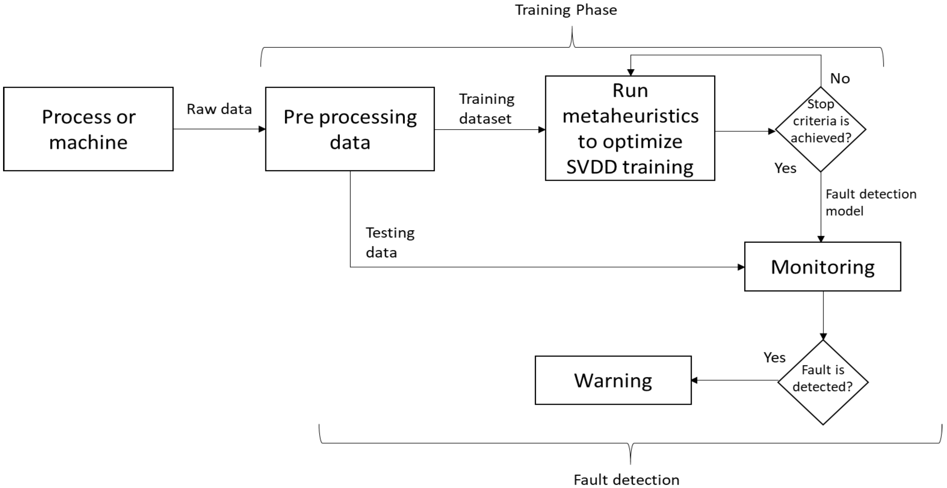
3. Methodology for Fault Detection
4. Industrial Application
5. Conclusions and Future Work
Author Contributions
Funding
Conflicts of Interest
References
- Ghaheri, A.; Shoar, S.; Naderan, M.; Hoseini, S. The Applications of Genetic Algorithms in Medicine. Oman Med. J. 2015, 30, 406–416. [Google Scholar] [CrossRef] [PubMed]
- Vats, S.; Dubey, S.K.; Pandey, N.K. Genetic algorithms for credit card fraud detection. In Proceedings of the International Conference on Education and Educational Technologies, Barcelona, Spain, 1–3 July 2013. [Google Scholar]
- Azzini, A.; De Felice, M.; Tettamanzi, A.G.B. A Comparison between Nature-Inspired and Machine Learning Approaches to Detecting Trend Reversals in Financial Time Series. In Natural Computing in Computational Finance: Volume 4; Brabazon, A., O’Neill, M., Maringer, D., Eds.; Springer: Berlin/Heidelberg, Germany, 2012; pp. 39–59. [Google Scholar] [CrossRef]
- Chiroma, H.; Gital, A.Y.; Rana, N.; Abdulhamid, S.M.; Muhammad, A.N.; Umar, A.Y.; Abubakar, A.I. Nature Inspired Meta-heuristic Algorithms for Deep Learning: Recent Progress and Novel Perspective. In Advances in Computer Vision; Arai, K., Kapoor, S., Eds.; Springer: Cham, Switzerland, 2020; pp. 59–70. [Google Scholar]
- Tao, Y.; Shi, H.; Song, B.; Tan, S. A Novel Dynamic Weight Principal Component Analysis Method and Hierarchical Monitoring Strategy for Process Fault Detection and Diagnosis. IEEE Trans. Ind. Electron. 2020, 67, 7994–8004. [Google Scholar] [CrossRef]
- Zhang, X.; Kano, M.; Li, Y. Principal Polynomial Analysis for Fault Detection and Diagnosis of Industrial Processes. IEEE Access 2018, 6, 52298–52307. [Google Scholar] [CrossRef]
- Amin, M.T.; Imtiaz, S.; Khan, F. Process system fault detection and diagnosis using a hybrid technique. Chem. Eng. Sci. 2018, 189, 191–211. [Google Scholar] [CrossRef]
- Wu, H.; Zhao, J. Deep convolutional neural network model based chemical process fault diagnosis. Comput. Chem. Eng. 2018, 115, 185–197. [Google Scholar] [CrossRef]
- Don, M.G.; Khan, F. Dynamic process fault detection and diagnosis based on a combined approach of hidden Markov and Bayesian network model. Chem. Eng. Sci. 2019, 201, 82–96. [Google Scholar] [CrossRef]
- Tax, D.M.; Duin, R.P. Support Vector Data Description. Mach. Learn. 2004, 54, 45–66. [Google Scholar] [CrossRef] [Green Version]
- Paturi, U.; Cheruku, S. Application and performance of machine learning techniques in manufacturing sector from the past two decades: A review. Mater. Today Proc. 2020. [Google Scholar] [CrossRef]
- Rostami, H.; Dantan, J.; Homri, L. Review of data mining applications for quality assessment in manufacturing industry: Support vector machines. Int. J. Metrol. Qual. Eng. 2015, 6, 401. [Google Scholar] [CrossRef] [Green Version]
- Orru, P.; Zoccheddu, A.; Sassu, L.; Mattia, C.; Cozza, R.; Arena, S. Machine learning approach using MLP and SVM algorithms for the fault prediction of a centrifugal pump in the oil and gas industry. Sustainability 2020, 12, 4776. [Google Scholar] [CrossRef]
- Giorgi, M.D.; Campilongo, S.; Ficarella, A. A diagnostics tool for aero-engines health monitoring using machine learning technique. Energy Procedia 2018, 148, 860–867. [Google Scholar] [CrossRef]
- Jiang, Z.; Hu, M.; Feng, K.; Wang, H. A SVDD and-Means Based Early Warning Method for Dual-Rotor Equipment under Time-Varying Operating Conditions. Shock Vib. 2018, 2018. [Google Scholar] [CrossRef] [Green Version]
- Jazi, A.Y.; Liu, J.J.; Lee, H. Automatic inspection of TFT-LCD glass substrates using optimized support vector machines. IFAC Proc. Vol. 2012, 45, 325–330. [Google Scholar] [CrossRef] [Green Version]
- Zhuang, L.; Dai, H. Parameter optimization of kernel-based one-class classifier on imbalance text learning. In Pacific Rim International Conference on Artificial Intelligence; Springer: Berlin/Heidelberg, Germany, 2006; pp. 434–443. [Google Scholar]
- Cao, Q.; Yu, L.; Cheng, M. A Brief Overview on Parameter Optimization of Support Vector Machine. DEStech Trans. Mater. Sci. Eng. 2016. [Google Scholar] [CrossRef] [Green Version]
- Zhang, X.; Chen, W.; Wang, B.; Chen, X. Intelligent fault diagnosis of rotating machinery using support vector machine with ant colony algorithm for synchronous feature selection and parameter optimization. Neurocomputing 2015, 167, 260–279. [Google Scholar] [CrossRef]
- Lessmann, S.; Stahlbock, R.; Crone, S.F. Genetic algorithms for support vector machine model selection. In Proceedings of the 2006 IEEE International Joint Conference on Neural Network, Vancouver, BC, Canada, 16–21 July 2006; pp. 3063–3069. [Google Scholar]
- Theissler, A.; Dear, I. Autonomously Determining the Parameters for SVDD with RBF Kernel from a One-Class Training Set. Int. J. Comput. Inf. Eng. 2013, 7, 949–957. [Google Scholar]
- Xiao, T.; Ren, D.; Lei, S.; Zhang, J.; Liu, X. Based on grid-search and PSO parameter optimization for Support Vector Machine. In Proceedings of the 11th World Congress on Intelligent Control and Automation, Shenyang, China, 29 June–4 July 2014; pp. 1529–1533. [Google Scholar]
- Panda, N.E.A. Oppositional Spotted Hyena Optimizer with Mutation Operator for Global Optimization and Application in Training Wavelet Neural Network. J. Intell. Fuzzy Syst. 2020. [Google Scholar] [CrossRef]
- Moayedi, H.; Bui, D.T.; Dounis, A.; Kalantar, B. Spotted Hyena Optimizer and Ant Lion Optimization in Predicting the Shear Strength of Soil. Appl. Sci. 2019, 9, 4738. [Google Scholar] [CrossRef] [Green Version]
- Dhiman, G.; Chahar, V. Spotted Hyena Optimizer for Solving Complex and Nonlinear Constrained Engineering Problems: Theory and Applications. In Harmony Search and Nature Inspired Optimization Algorithms; Springer: Singapore, 2019. [Google Scholar]
- Dhiman, G.; Kaur, A. Optimizing the Design of Airfoil and Optical Buffer Problems Using Spotted Hyena Optimizer. Designs 2018, 2, 28. [Google Scholar] [CrossRef] [Green Version]
- Chahar, V.; Kaur, A. Binary Spotted Hyena Optimizer and its Application to Feature Selection. J. Ambient. Intell. Humaniz. Comput. 2019, 11, 2625–2645. [Google Scholar]
- Dhiman, G.; Kaur, A. A Hybrid Algorithm Based on Particle Swarm and Spotted Hyena Optimizer for Global Optimization. In Soft Computing for Problem Solving; Bansal, J.C., Das, K.N., Nagar, A., Deep, K., Ojha, A.K., Eds.; Springer: Singapore, 2019; pp. 599–615. [Google Scholar]
- Divya, S.; El, K.; Rao, M.; Vemulapati, P. Prediction of Gene Selection Features Using Improved Multi-objective Spotted Hyena Optimization Algorithm. In Data Communication and Networks; Springer: Singapore, 2020. [Google Scholar]
- Gandomi, A.H.; Alavi, A.H. Krill herd: A new bio-inspired optimization algorithm. Commun. Nonlinear Sci. Numer. Simul. 2012, 17, 4831–4845. [Google Scholar] [CrossRef]
- Bolaji, A.L.; Al-Betar, M.A.; Awadallah, M.A.; Khader, A.T.; Abualigah, L.M. A comprehensive review: Krill Herd algorithm (KH) and its applications. Appl. Soft Comput. 2016, 49, 437–446. [Google Scholar] [CrossRef]
- Abualigah, L.M.; Khader, A.T.; Al-Betar, M.A.; Awadallah, M.A. A krill herd algorithm for efficient text documents clustering. In Proceedings of the 2016 IEEE Symposium on Computer Applications & Industrial Electronics (ISCAIE), Batu Feringghi, Malaysia, 30–31 May 2016; pp. 67–72. [Google Scholar]
- Abualigah, L.M.; Khader, A.T.; Hanandeh, E.S.; Gandomi, A.H. A novel hybridization strategy for krill herd algorithm applied to clustering techniques. Appl. Soft Comput. 2017, 60, 423–435. [Google Scholar] [CrossRef]
- Abualigah, L.M.; Khader, A.T.; Hanandeh, E.S. A combination of objective functions and hybrid krill herd algorithm for text document clustering analysis. Eng. Appl. Artif. Intell. 2018, 73, 111–125. [Google Scholar] [CrossRef]
- Abualigah, L.M.; Khader, A.T.; Hanandeh, E.S. Hybrid clustering analysis using improved krill herd algorithm. Appl. Intell. 2018, 48, 4047–4071. [Google Scholar] [CrossRef]
- Karthick, P.; Palanisamy, C. Optimized cluster head selection using krill herd algorithm for wireless sensor network. Automatika 2019, 60, 340–348. [Google Scholar] [CrossRef] [Green Version]
- Wang, Z.; Zheng, L.; Wang, J.; Du, W. Research on novel bearing fault diagnosis method based on improved krill herd algorithm and kernel extreme learning machine. Complexity 2019, 2019. [Google Scholar] [CrossRef]
- Zhang, Y.; Li, X.; Zheng, H.; Yao, H.; Liu, J.; Zhang, C.; Peng, H.; Jiao, J. A fault diagnosis model of power transformers based on dissolved gas analysis features selection and improved krill herd algorithm optimized support vector machine. IEEE Access 2019, 7, 102803–102811. [Google Scholar] [CrossRef]
- Jain, M.; Singh, V.; Rani, A. A novel nature-inspired algorithm for optimization: Squirrel search algorithm. Swarm Evol. Comput. 2019, 44, 148–175. [Google Scholar] [CrossRef]
- Zheng, T.; Luo, W. An improved squirrel search algorithm for optimization. Complexity 2019, 2019. [Google Scholar] [CrossRef]
- Altamirano-Guerrero, G.; Garcia-Calvillo, I.D.; Resendiz-Flores, E.O.; Costa, P.; Salinas-Rodriguez, A.; Goodwin, F. Intelligent design in continuous galvanizing process for advanced ultra-high-strength dual-phase steels using back-propagation artificial neural networks and MOAMP-Squirrels search algorithm. Int. J. Adv. Manuf. Technol. 2020, 110, 2619–2630. [Google Scholar] [CrossRef]
- Basu, M. Squirrel search algorithm for multi-region combined heat and power economic dispatch incorporating renewable energy sources. Energy 2019, 182, 296–305. [Google Scholar] [CrossRef]
- Hu, H.; Zhang, L.; Bai, Y.; Wang, P.; Tan, X. A hybrid algorithm based on squirrel search algorithm and invasive weed optimization for optimization. IEEE Access 2019, 7, 105652–105668. [Google Scholar] [CrossRef]
- Sanaj, M.; Prathap, P.J. Nature inspired chaotic squirrel search algorithm (CSSA) for multi objective task scheduling in an IAAS cloud computing atmosphere. Eng. Sci. Technol. Int. J. 2020, 23, 891–902. [Google Scholar] [CrossRef]
- Shen, F.; Song, Z.; Zhou, L. Improved PCA-SVDD based monitoring method for nonlinear process. In Proceedings of the 2013 25th Chinese Control and Decision Conference (CCDC), Guiyang, China, 25–27 May 2013; pp. 4330–4336. [Google Scholar] [CrossRef]
- Yin, G.; Zhang, Y.T.; Li, Z.N.; Ren, G.Q.; Fan, H.B. Online fault diagnosis method based on Incremental Support Vector Data Description and Extreme Learning Machine with incremental output structure. Neurocomputing 2014, 128, 224–231. [Google Scholar] [CrossRef]
- Liu, C.; Gryllias, K. A semi-supervised Support Vector Data Description-based fault detection method for rolling element bearings based on cyclic spectral analysis. Mech. Syst. Signal Process. 2020, 140, 106682. [Google Scholar] [CrossRef]
- Dhiman, G.; Chahar, V. Spotted Hyena Optimizer: A Novel Bio-inspired based Metaheuristic Technique for Engineering Applications. Adv. Eng. Softw. 2017. [Google Scholar] [CrossRef]
- Kennedy, J.; Eberhart, R.C. Particle Swarm Optimization. IEEE Int. Conf. Neural Netw. 1995, 4, 1942–1948. [Google Scholar]
- Abualigah, L.M.; Khader, A.T.; Hanandeh, E.S. A new feature selection method to improve the document clustering using particle swarm optimization algorithm. J. Comput. Sci. 2018, 25, 456–466. [Google Scholar] [CrossRef]
- Abdi, L.J.W.H. Encyclopedia of Research Design; SAGE Publications: New York, NY, USA, 2010. [Google Scholar]


| Description | |
|---|---|
| [], Nozzle 1 | |
| [], Nozzle 2 | |
| [Percent], Heating power zone 1 | |
| [Percent], Heating power zone 2 | |
| [Percent], Heating power zone 3 | |
| [Percent], Heating power zone 4 | |
| [Percent], Heating power zone 5 | |
| [Percent], Heating power zone 6 | |
| [in], Mold position value | |
| [in], Opening run | |
| [US ton], Closing force peak value | |
| [US ton], Closing force real value | |
| [s], Mold protection time | |
| [], Oil temperature | |
| [], Traverse | |
| [s], Cooling time | |
| [psi], Backpressure | |
| [], Volume end screw | |
| holding pressure | |
| [psi], Holding pressure | |
| [/s], Dosage power | |
| [psi], Pressure at Switchover | |
| [s], Cycle time | |
| [lbf-ft], Mean spin | |
| [lbf-ft], Peak value at spin | |
| [psi], Specific injection pressure | |
| [], Dosage volume | |
| [], Injection volume | |
| [s], Dosing time | |
| [s], Injection time | |
| [], Cylinder zone 1 | |
| [], Cylinder zone 2 | |
| [], Cylinder zone 3 | |
| [], Cylinder zone 4 | |
| [ft/s], Revolutions | |
| [Wh], Injection work | |
| [], Switching volume |
| SHO | KH | SSA | PSO | |
|---|---|---|---|---|
| Number of iterations | 200 | 200 | 200 | 200 |
| Population size | 50 | 50 | 50 | 50 |
| , | ||||
| Other parameters | , | , | ||
| F1 Score | Time | |||||||
|---|---|---|---|---|---|---|---|---|
| SHO | KH | SSA | PSO | SHO | KH | SSA | PSO | |
| 1 | 0.9620 | 0.9189 | 0.9610 | 0.9189 | 76.6396 | 112.7972 | 139.2550 | 207.6410 |
| 2 | 0.9744 | 0.9189 | 0.9189 | 0.9189 | 78.2157 | 114.3666 | 149.3458 | 209.0972 |
| 3 | 0.9512 | 0.9189 | 0.9750 | 0.9189 | 77.4362 | 113.8831 | 129.8195 | 208.6143 |
| 4 | 0.9744 | 0.9189 | 0.9189 | 0.9189 | 77.4033 | 113.4381 | 149.1254 | 208.5458 |
| 5 | 0.9744 | 0.9189 | 0.9189 | 0.9189 | 77.6753 | 114.3179 | 147.2649 | 207.9583 |
| 6 | 0.9750 | 0.9189 | 0.9189 | 0.9189 | 76.9510 | 113.6539 | 155.0708 | 209.6714 |
| 7 | 0.9744 | 0.9189 | 0.9744 | 0.9189 | 77.3957 | 114.0773 | 142.7828 | 211.6702 |
| 8 | 0.9750 | 0.9189 | 0.9750 | 0.9333 | 79.0279 | 113.6960 | 128.8649 | 212.5049 |
| 9 | 0.9750 | 0.9189 | 0.9189 | 0.9189 | 78.7634 | 113.6895 | 143.1924 | 208.9668 |
| 10 | 0.9744 | 0.9189 | 0.9211 | 0.9189 | 83.3741 | 113.5960 | 142.3234 | 209.6382 |
| 11 | 0.9630 | 0.9189 | 0.9750 | 0.9189 | 80.4753 | 113.8772 | 116.8845 | 210.7641 |
| 12 | 0.9750 | 0.9189 | 0.9189 | 0.9189 | 82.3348 | 114.1014 | 151.0041 | 209.1223 |
| 13 | 0.9750 | 0.9189 | 0.9189 | 0.9189 | 79.5617 | 114.0026 | 149.3981 | 208.3499 |
| 14 | 0.9750 | 0.9189 | 0.9189 | 0.9189 | 78.9463 | 114.1080 | 146.5968 | 208.5490 |
| 15 | 0.9750 | 0.9189 | 0.9189 | 0.9189 | 79.7457 | 113.7620 | 151.1163 | 210.4518 |
| 16 | 0.9744 | 0.9189 | 0.9351 | 0.9189 | 88.0263 | 113.7218 | 135.8897 | 209.4198 |
| 17 | 0.9512 | 0.9189 | 0.9189 | 0.9189 | 78.0516 | 113.8042 | 147.1367 | 209.8243 |
| 18 | 0.9620 | 0.9189 | 0.9189 | 0.9189 | 77.6847 | 113.7368 | 147.1347 | 213.8261 |
| 19 | 0.9744 | 0.9744 | 0.9189 | 0.9189 | 77.9648 | 98.1384 | 145.6228 | 208.7176 |
| 20 | 0.9620 | 0.9744 | 0.9189 | 0.9189 | 79.1865 | 114.2702 | 152.3700 | 208.1235 |
| 21 | 0.9744 | 0.9744 | 0.9189 | 0.9189 | 79.1609 | 114.2038 | 146.7939 | 209.6390 |
| 22 | 0.9750 | 0.9744 | 0.9189 | 0.9189 | 76.4243 | 114.1394 | 148.8082 | 210.0689 |
| 23 | 0.9630 | 0.9744 | 0.9189 | 0.9189 | 76.2201 | 113.5049 | 147.7095 | 207.0849 |
| 24 | 0.9750 | 0.9744 | 0.9189 | 0.9189 | 78.9390 | 113.6086 | 145.8267 | 208.5851 |
| 25 | 0.9750 | 0.9744 | 0.9189 | 0.9189 | 75.2608 | 113.7726 | 149.5031 | 225.5017 |
| 26 | 0.9744 | 0.9744 | 0.9744 | 0.9189 | 74.3404 | 113.8676 | 129.5610 | 210.0427 |
| 27 | 0.9744 | 0.9744 | 0.9189 | 0.9189 | 74.6434 | 114.3396 | 148.6370 | 207.7600 |
| 28 | 0.9620 | 0.9744 | 0.9750 | 0.9189 | 74.9797 | 113.4536 | 131.1206 | 209.6813 |
| 29 | 0.9620 | 0.9750 | 0.9189 | 0.9189 | 74.6099 | 93.0891 | 154.4285 | 207.8903 |
| 30 | 0.9750 | 0.9750 | 0.9189 | 0.9189 | 76.3885 | 114.4280 | 157.7352 | 213.1721 |
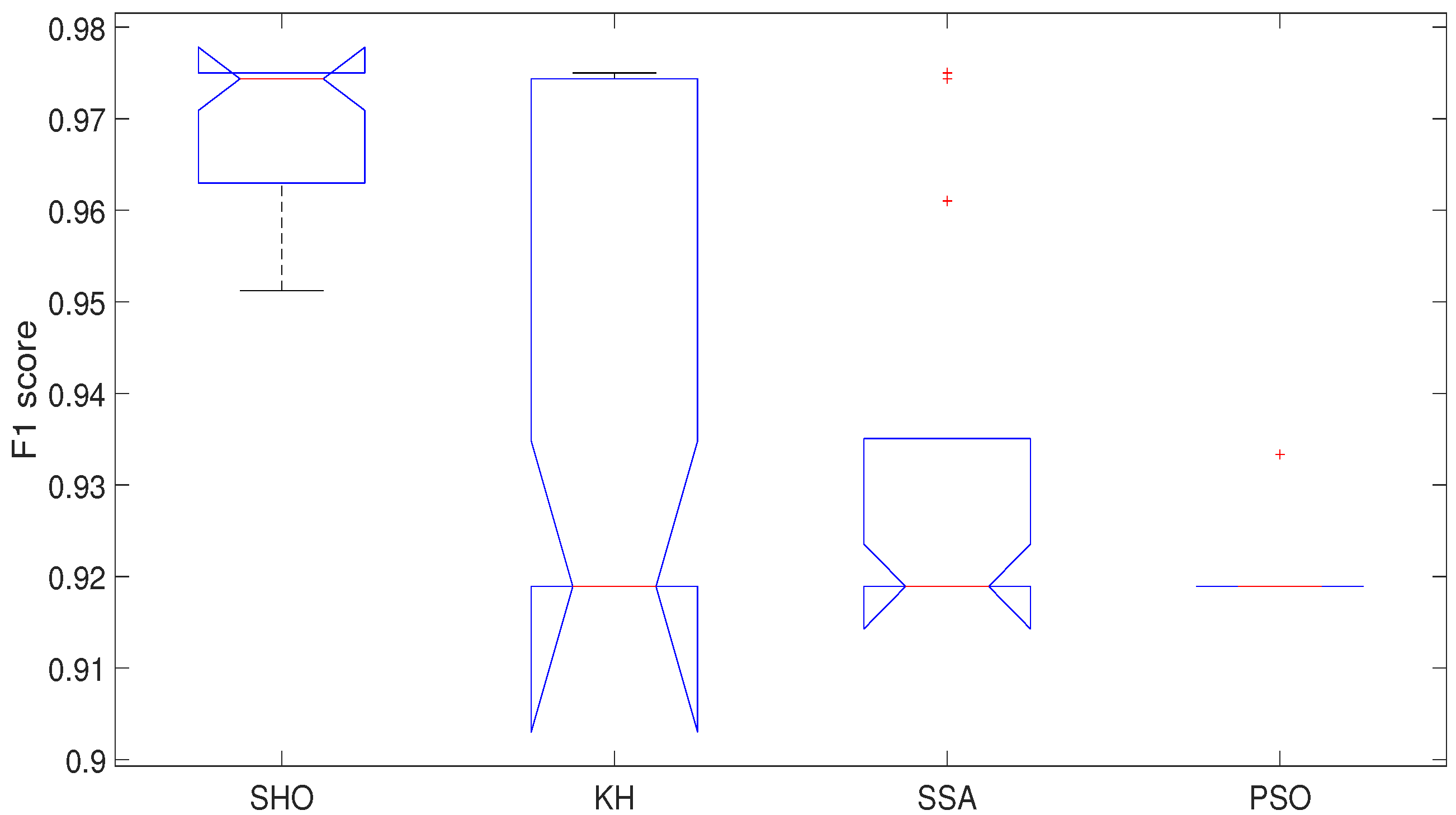
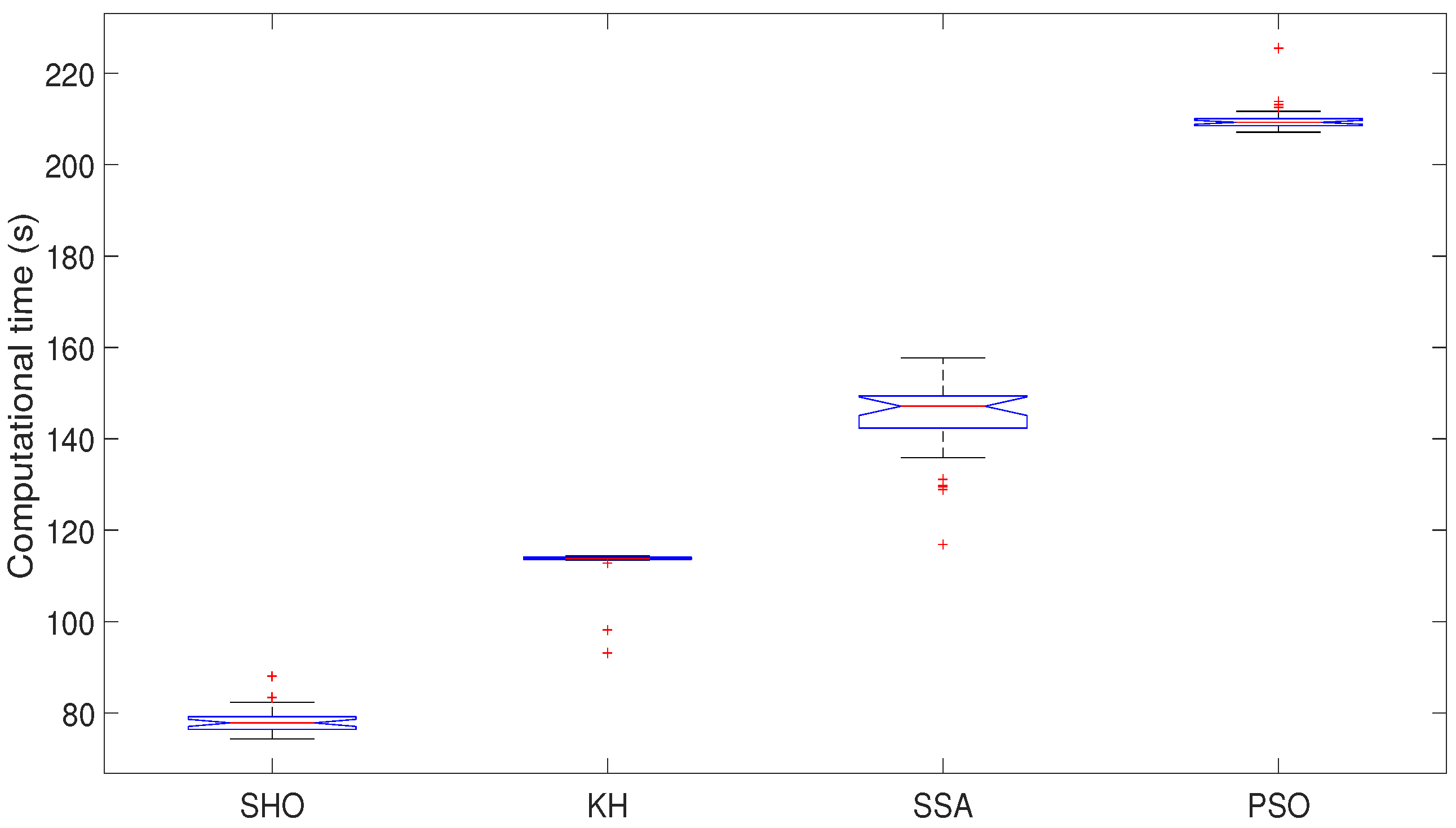
| Mean | 0.9702 | 0.9411 | 0.9321 | 0.9194 | 78.1942 | 112.6482 | 144.3441 | 210.0294 |
| Std | 0.0074 | 0.0277 | 0.0232 | 0.0026 | 2.8170 | 4.6904 | 9.1777 | 3.3325 |
| Source | SS | df | MS | Chi-sq | p-Value |
|---|---|---|---|---|---|
| Columns | 56,089.6 | 3 | 18,696.5 | 57.3 | 2.2188 |
| Error | 60,398.9 | 116 | 520.7 | ||
| Total | 116,488.5 | 119 |
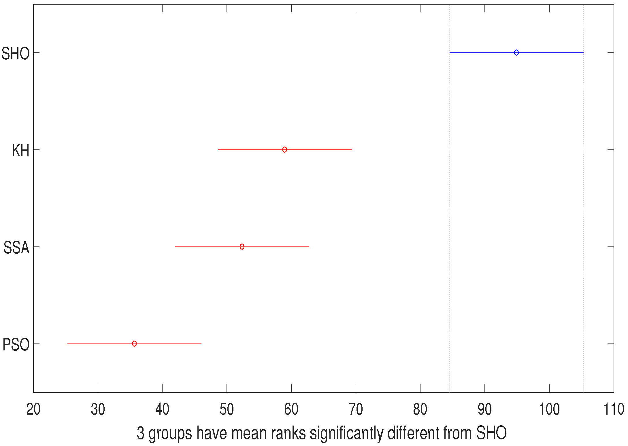
| Source | SS | df | MS | Chi-sq | p-Value |
|---|---|---|---|---|---|
| Columns | 135,000 | 3 | 45,000 | 111.57 | 5.0394 |
| Error | 8990 | 116 | 77.5 | ||
| Total | 143,990 | 119 |
Publisher’s Note: MDPI stays neutral with regard to jurisdictional claims in published maps and institutional affiliations. |
© 2020 by the authors. Licensee MDPI, Basel, Switzerland. This article is an open access article distributed under the terms and conditions of the Creative Commons Attribution (CC BY) license (http://creativecommons.org/licenses/by/4.0/).
Share and Cite
Navarro-Acosta, J.A.; García-Calvillo, I.D.; Avalos-Gaytán, V.; Reséndiz-Flores, E.O. Metaheuristics and Support Vector Data Description for Fault Detection in Industrial Processes. Appl. Sci. 2020, 10, 9145. https://0-doi-org.brum.beds.ac.uk/10.3390/app10249145
Navarro-Acosta JA, García-Calvillo ID, Avalos-Gaytán V, Reséndiz-Flores EO. Metaheuristics and Support Vector Data Description for Fault Detection in Industrial Processes. Applied Sciences. 2020; 10(24):9145. https://0-doi-org.brum.beds.ac.uk/10.3390/app10249145
Chicago/Turabian StyleNavarro-Acosta, Jesús Alejandro, Irma D. García-Calvillo, Vanesa Avalos-Gaytán, and Edgar O. Reséndiz-Flores. 2020. "Metaheuristics and Support Vector Data Description for Fault Detection in Industrial Processes" Applied Sciences 10, no. 24: 9145. https://0-doi-org.brum.beds.ac.uk/10.3390/app10249145