Research on Vehicle Trajectory Prediction and Warning Based on Mixed Neural Networks

Featured Application

The potential applications of car trajectory prediction include self-driving and vehicle warning systems.

Abstract

When driving on roads, the most important issue for driving is safety. There are various vehicles, including cars, motorcycles, bicycles, and pedestrians, that increase the complexity of road conditions and the burden on drivers. In order to improve driving safety, a deep learning framework is applied to predict and announce the trajectory of a car. This research is divided into three parts. Lane line detection is adopted first. Secondly, car object detection is employed. Lastly, car trajectory prediction is a key part of our research. In addition, real images and videos in the driving recorder are used to simulate the real situation the driver sees from the driver’s seat. Car detection is utilized to obtain the coordinates of the car in these images, reaching an accuracy of 0.91 and then predicting the future trajectory of the car, obtaining a loss of 0.00024 and costing 12 milliseconds. It can precisely mark the position of the car, accurately detect the lane line, and predict the future car’s trajectory. Through the prediction and announcement of the car trajectory, we verified that our model can correctly predict the car trajectory and truly enhance the safety of driving.

1. Introduction

The most significant aspect of driving is the safety of the driver. Vehicle accidents are sometimes unpredictable and happen suddenly. For instance, if someone violates traffic regulations, it greatly increases the probability of a vehicle accident. Therefore, we may encounter these terrible things even if we drive cautiously on the road. In this paper, at first, a traditional method [1] is used to predict the future location of objects. However, the traditional method is not suitable for complex predictions. In recent years, deep neural networks (DNNs) have been applied to process trajectory prediction, demonstrating impressive results [2,3]. Almost all of these approaches are based on recurrent neural networks (RNNs) [4], since a trajectory is a temporal sequence. RNNs can share parameters across a time sequence, but they cannot handle long-term dependencies, because RNNs will always retain previous information.

To improve the problem of RNNs, a long short-term memory (LSTM) network was designed [5]. LSTM is a kind of RNN architecture that contains three special gates for controlling information. In [6], the authors used an LSTM network to predict the trajectory of the car on the highway, and it showed excellent results of the predicted trajectory. The LSTM network is used to build temporal and spatial attention models, which can predict trajectory well [7]. Beyond the traditional LSTM, it is necessary to integrate more information on the road, such as our proposed new warning system for object detection and the prediction of the X and Y coordinates of the car. In [6], only an LSTM network is used to predict lateral position and longitudinal velocity of the car on highways. In this paper, we revised the architecture of the LSTM network to give drivers more important information by combining multiple models. The prediction results were as good as those in [6], but our proposed method could obtain more information about the road. In [7], the authors used social LSTM with a spatial attention model and trajectory attention model to predict the car trajectory. In [8], LSTM encoder–decoder neural network architecture was used. In [9], object detection was used to track an object. Our proposed method could reach 10.995 frames per second (FPS), which was better than the 3 FPS achieved in [9]. Without the complex structure in [7,8], an efficient LSTM-based model was proposed and realized. The performance was as good as that in [7,8,9], but it took very little time to train and test our model. In addition, our proposed method contained multiple models to give more valuable information, which could detect quickly, warn the drivers, and improve driving safety.

In this paper, our aim was to use multiple models to build a system that could predict and warn. A method combining object detection of a car, lane line detection, and trajectory prediction of the car was proposed.

Object detection of a car is capable of detecting the car, which can help us distinguish the car on the road. YOLO (you only look once) [10,11] has excellent results in object detection. Furthermore, YOLO object detection is easy to train to some extent. It is not only accurate but also takes very little time for detection.

Lane line detection can find the lane line on the road. An improved Hough transform method [12], which uses wavelet, canny, and the Hough transform to detect lane lines, shows good correctness and real-time performance for lane line detection. In [13], a novel formulation was used and a structural loss was proposed, achieving state-of-the-art performance in terms of both speed and accuracy. We used a simple method based on OpenCV [14] for lane line detection. This technique assists the drivers to drive in the appropriate lane area, thereby reducing the chances of accidents. It can also detect the direction of the steering wheel to the left, the right, or straight ahead.

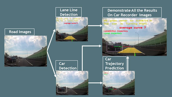
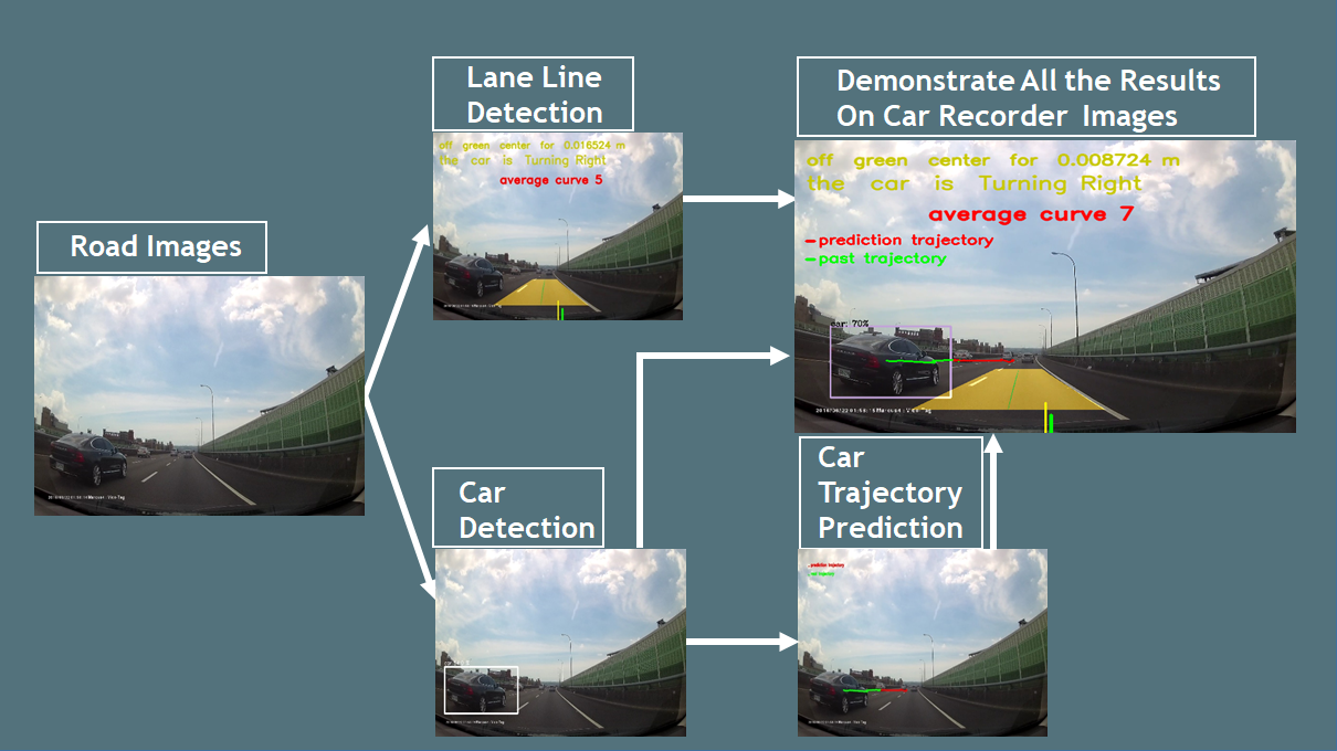
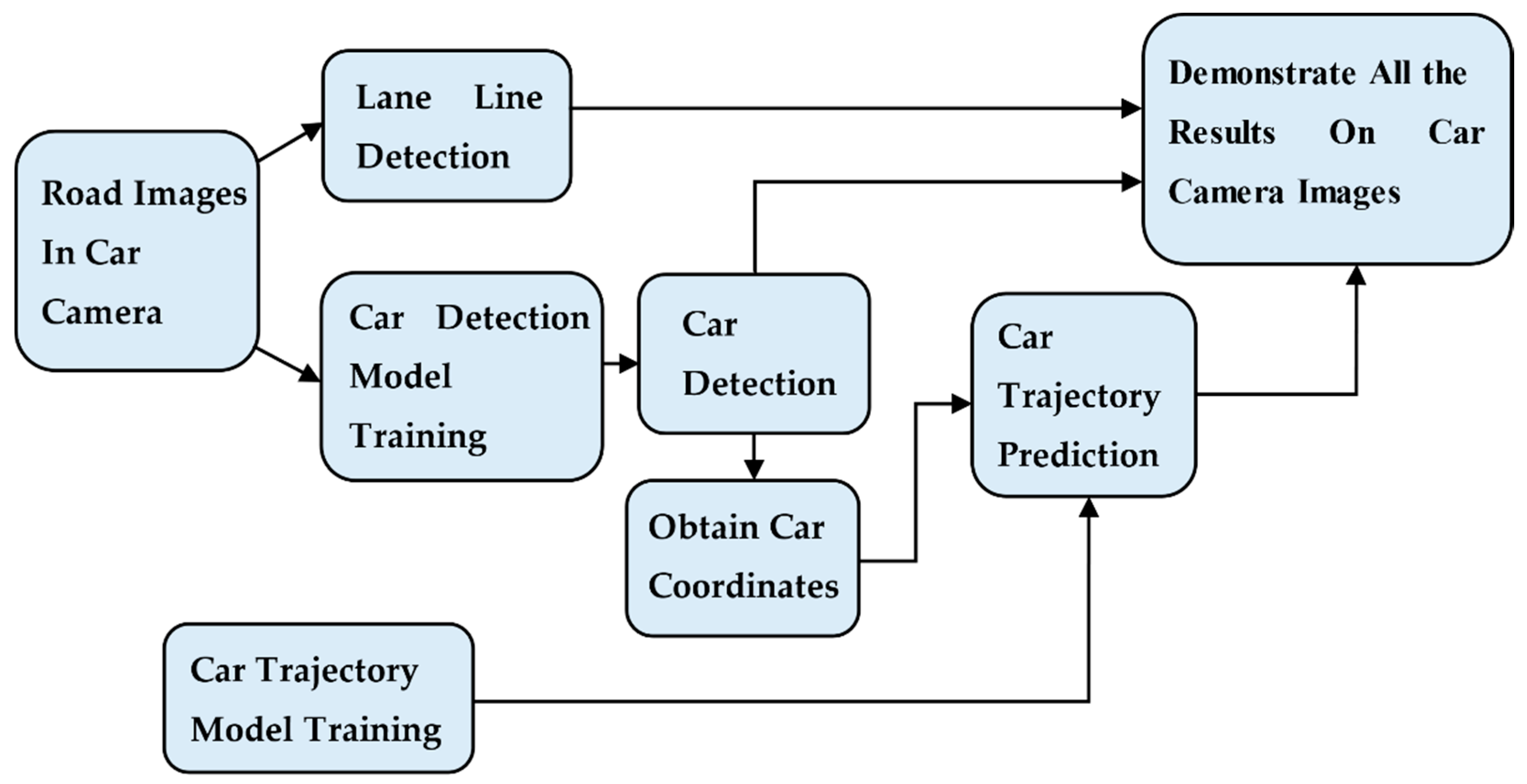
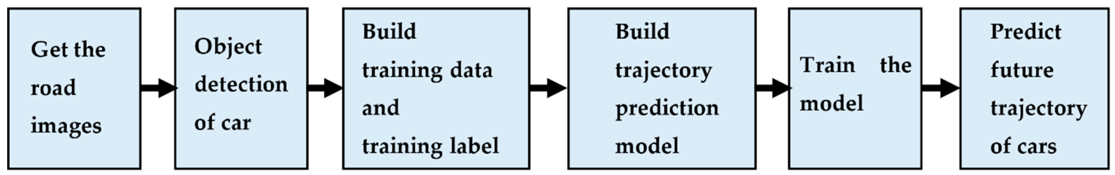
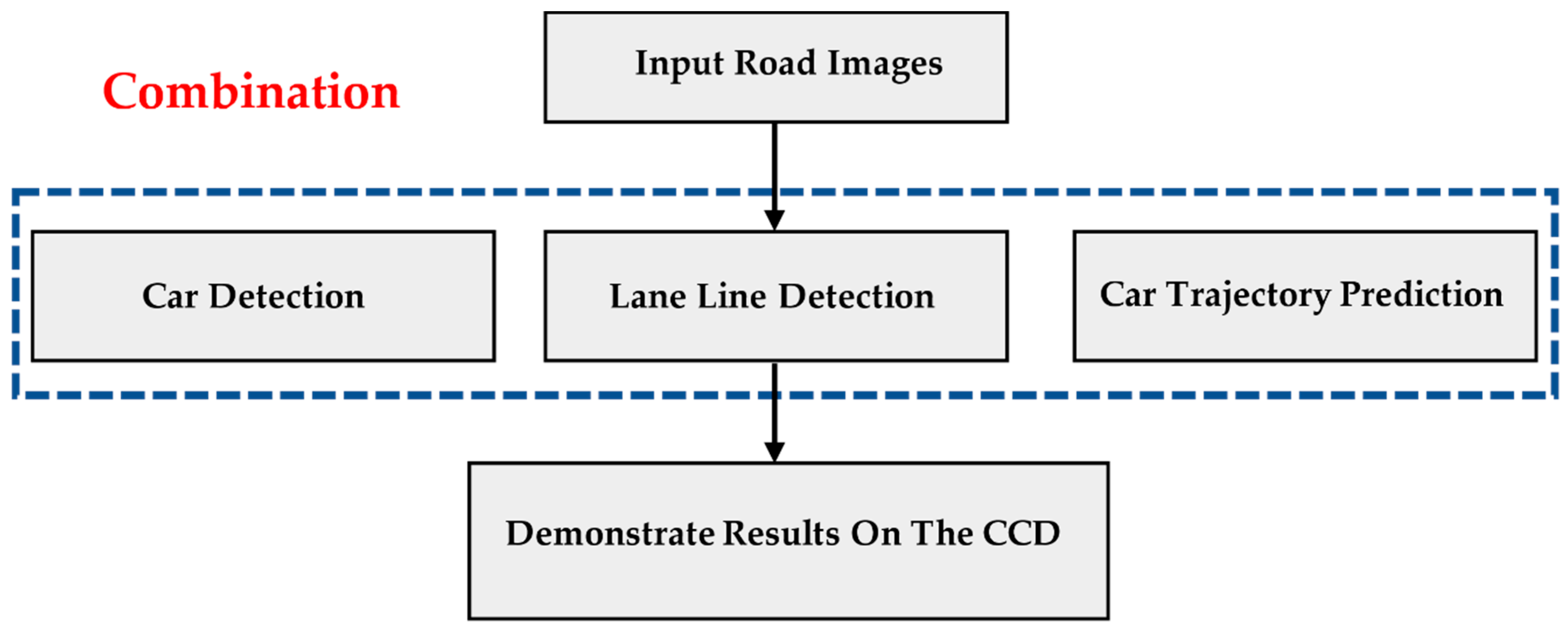
The crucial part of this research is trajectory prediction of a car. We retained the idea of [6] and proposed a new prediction model based on an LSTM structure [5,15]. If we could predict the possible trajectory of the car, we could preventively slow it down or take other suitable measures. At last, we combined all these techniques together. It was through the combination of multiple models that our system could detect cars and lane lines and predict the future trajectory of the car, showing good prediction and improving driving safety. Figure 1 shows the proposed framework of this research.

The rest of the paper is organized as follows. In Section 2, we review the materials on YOLO and LSTM, particularly in the process and structure. Section 3 describes our proposed approach and model design. Section 4 demonstrates the experiment results and presents the analysis and future prospects. We then conclude the paper in Section 5.

2. Related Works

2.1. Object Detection of a Car

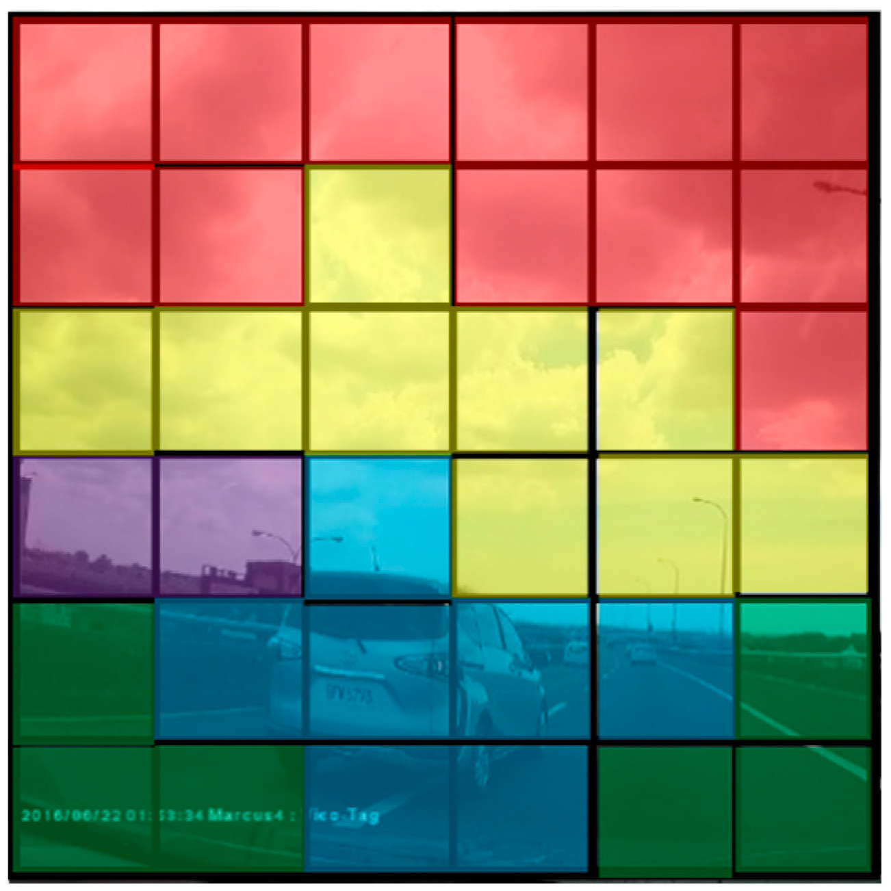
You only look once (YOLO) [10] is a machine learning (ML) framework for object detection, which attempts to detect any object depending on what is used to train the detection model. YOLO object detection can detect the location and the class of the object in the input image by carrying out one calculation of convolutional neural networks. In the first place, the input images are divided into S × S squares, which are called grid cells. As shown in Figure 2, there are 6 × 6 grid cells in Figure 2. Secondly, the prediction of the bounding box must be applied after the grid cells in the image are obtained. Each grid cell must process a fixed amount of prediction of the bounding box and confidence score. There are five values in each bounding box, including x, y, w, h, and confidence. The x, y value is the center of the bounding box, and w and h are the width and height, respectively, of the bounding box. The confidence is the value of intersection over union (IOU). The confidence score represents the probability of the bounding box that may contain the object. The confidence score will be zero if the bounding box does not contain an object. After predicting the bounding box, it will abandon redundant bounding boxes by the threshold method and the non-maximum suppression (NMS) method. The above operation is the method used to detect the location of the object in the image. Lastly, the class of the bounding box must be predicted. In this process, the class probability map must be used (Figure 3).

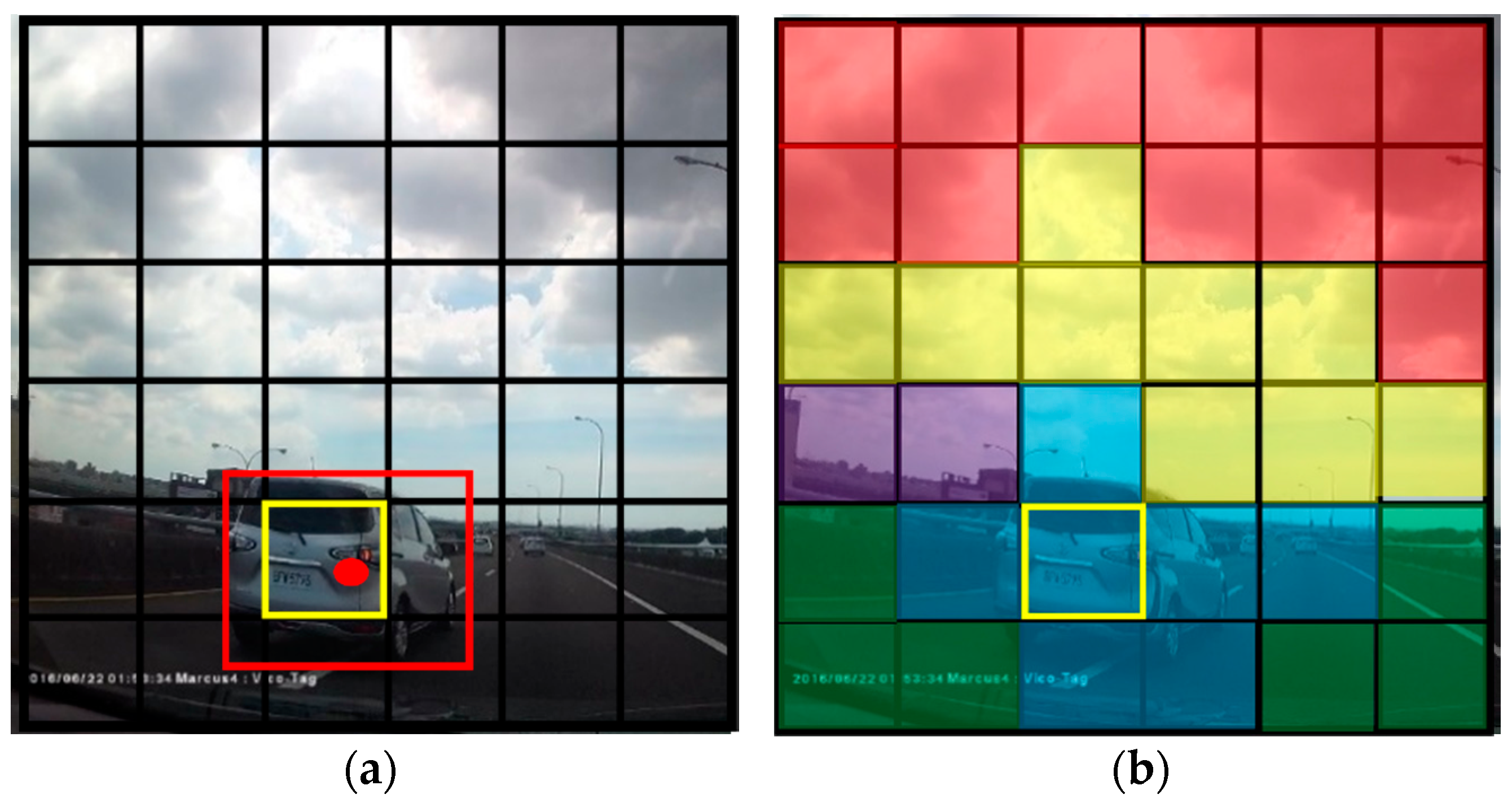
In this map, each color region represents one specific class. Using the blue region as an example, the blue region can be regarded as the car class in this class probability map. The class of the bounding box can then be predicted. The predicted bounding box is used in the second step. Then it can be compared with the class probability map. Figure 4 shows how to decide the class of the bounding box. Because the center of the bounding box is within the yellow grid cell, the yellow grid cell has to predict the bounding box. Thus, the only thing that must be done is to compare the left image to the right class map. Note that the yellow grid cell is inside the blue region, and we can assume that its class is a car. Finally, we can say that the red bounding box contains the car object. The object detection process is thus ended.

There are various improvements and extensions in YOLOv2 [11], while it also still predicts objects based on the above process. There are many crucial factors to enhance the accuracy of the model. YOLOv2 uses batch normalization, anchor boxes, and k-means, and removes two fully connected layers.

By adding these features into the model, the accuracy is increased and the detecting time is decreased.

2.2. Long Short-Term Memory

Long short-term memory (LSTM) [15] is a kind of recurrent neural network (RNN) [16], which is the optimal choice for addressing the problem of time sequences, for instance predicting the stock price for the next week. The share price must be changed every weekday. Thus, the stock price will change as time passes by every day, in which each time sequence can represent one specific value of the stock price. LSTM and RNN are the most suitable for conducting the problem of time sequences.

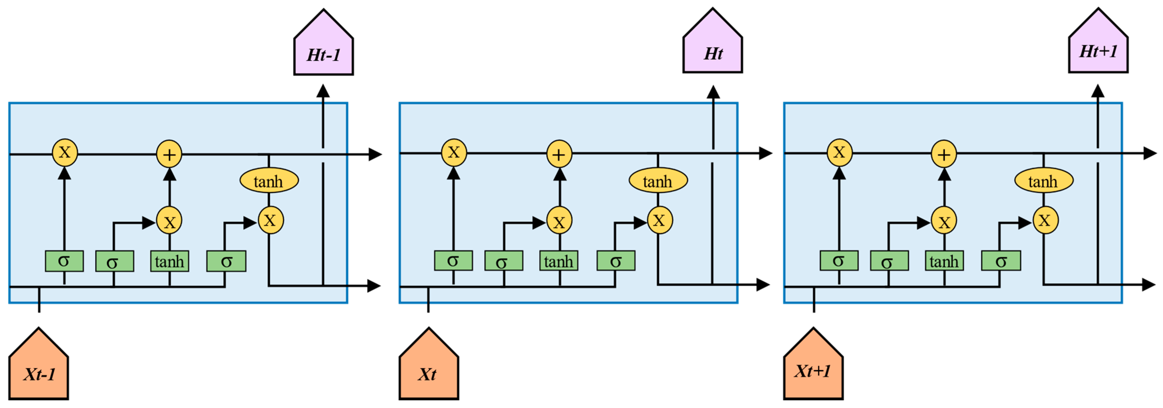
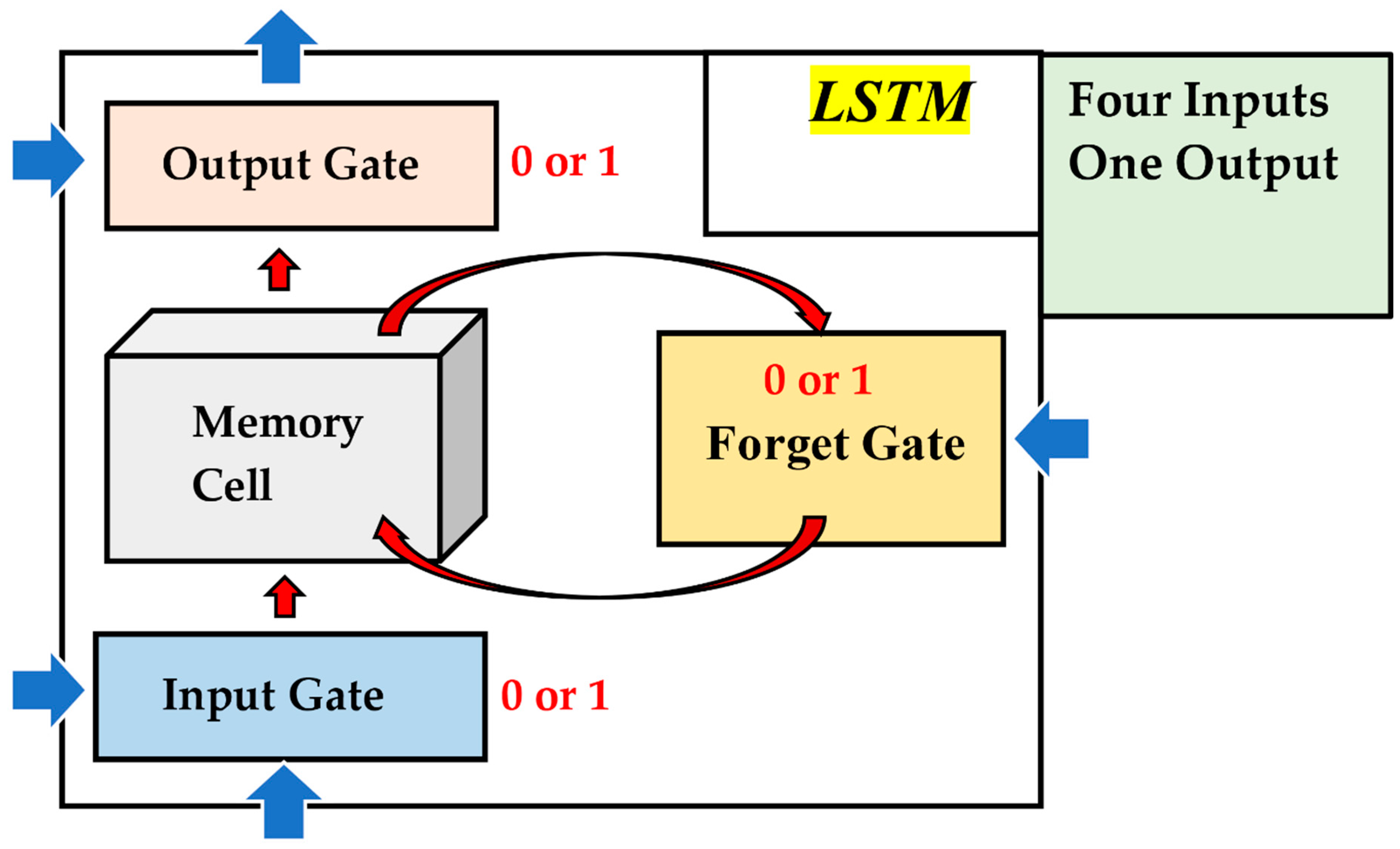
LSTM is the improved version of RNN. The structure of LSTM is shown in Figure 5 [17]. There are three specific features in the LSTM structure, including input gate, output gate, and forget gate (Figure 6). The major tasks of the gates are controlled by the LSTM, namely whether to abandon the history data, whether to let the data of new time sequences enter, and what data to output.

The process of LSTM consists of three stages. In the first stage, the forget gate operates, making the decision to either keep or discard the last time sequence data. The forget gate compares the history data with the new input data and eventually makes a choice. Next, the input gate controls what new data is allowed to pass through. Finally, the output gate determines the content of the output data. All these three gates are sigmoid activation layers. The sigmoid value is either zero or one. If the sigmoid value is zero, the gate will close. When the sigmoid value is one, the gate will open.

The above is the process of LSTM, and we can find that LSTM is very appropriate to handle the problem of time sequences. In addition, the model of LSTM can learn rapidly by controlling three gates. Due to the particular structure of the LSTM model, the LSTM model is easier to train than the RNN model.

3. Methods and Design

In our proposed method, we used multiple models. We applied Darkflow [18] only to process object detection of the car, and we did not change any of its parameters. In lane line detection, we used the simple method of OpenCV [14] for lane line detection. For car trajectory prediction, we proposed a new structure based on the LSTM model. In the end, we combined all of these and completed our forecasting system.

3.1. Object Detection of the Car

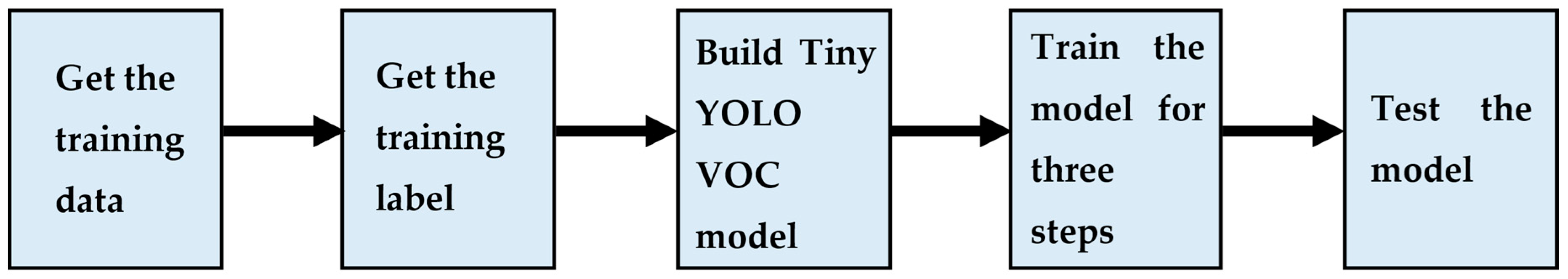
In this section, we discuss our training data, our car object detection model structure, and the training of the model. Our methods are demonstrated in the following sections. A flow-chart of object detection of the car is shown in Figure 7. The images from the car camera were used as our training data, and we applied labelImg [19] to obtain the training labels in the form of xml files. In addition, we built the object detection model of cars and trained the model in three steps. Finally, we used road images and videos to validate and evaluate the model.

3.1.1. Training Data Set

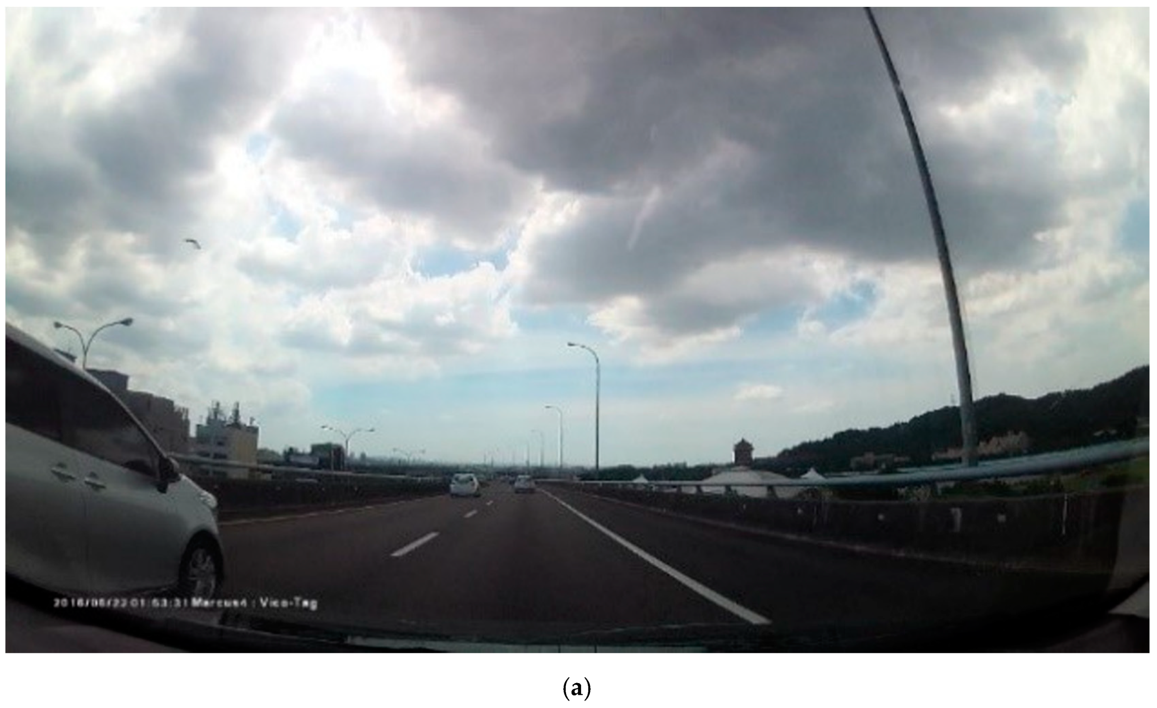
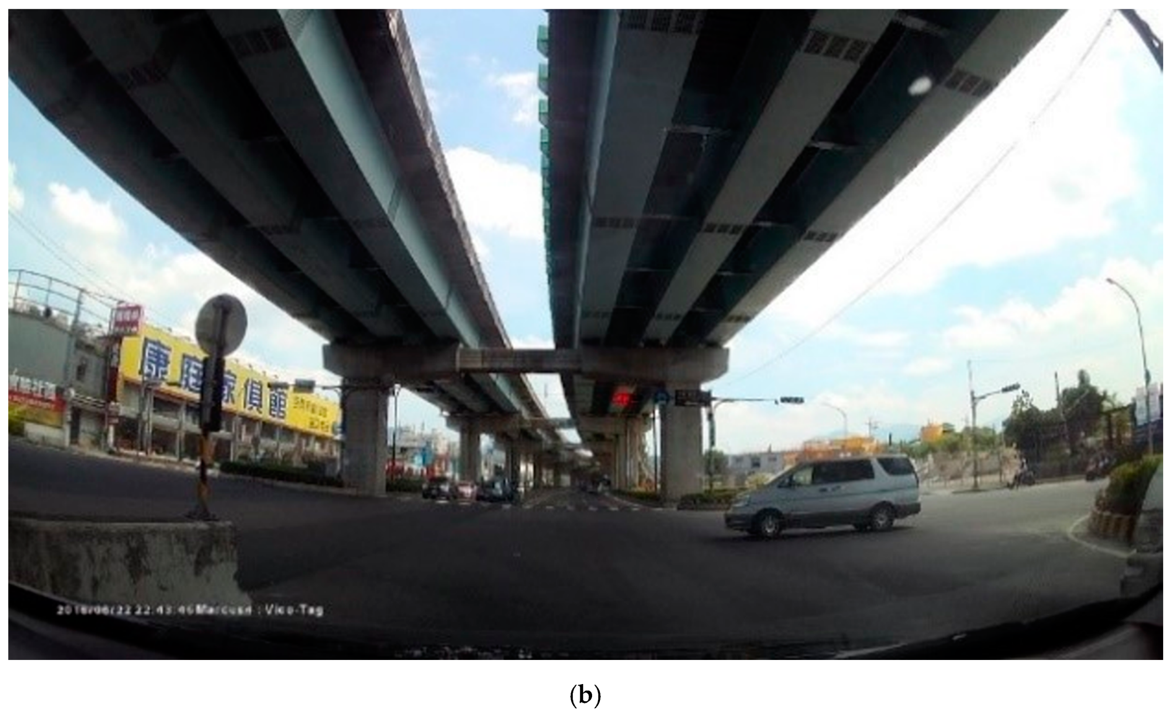
We obtained real videos of roads from our car recorder. After obtaining the videos, we transformed them into the form of an image. Figure 8 shows, by way of example, the ground truth road images that we recorded on a highway and urban road. We utilized these images as our training data.

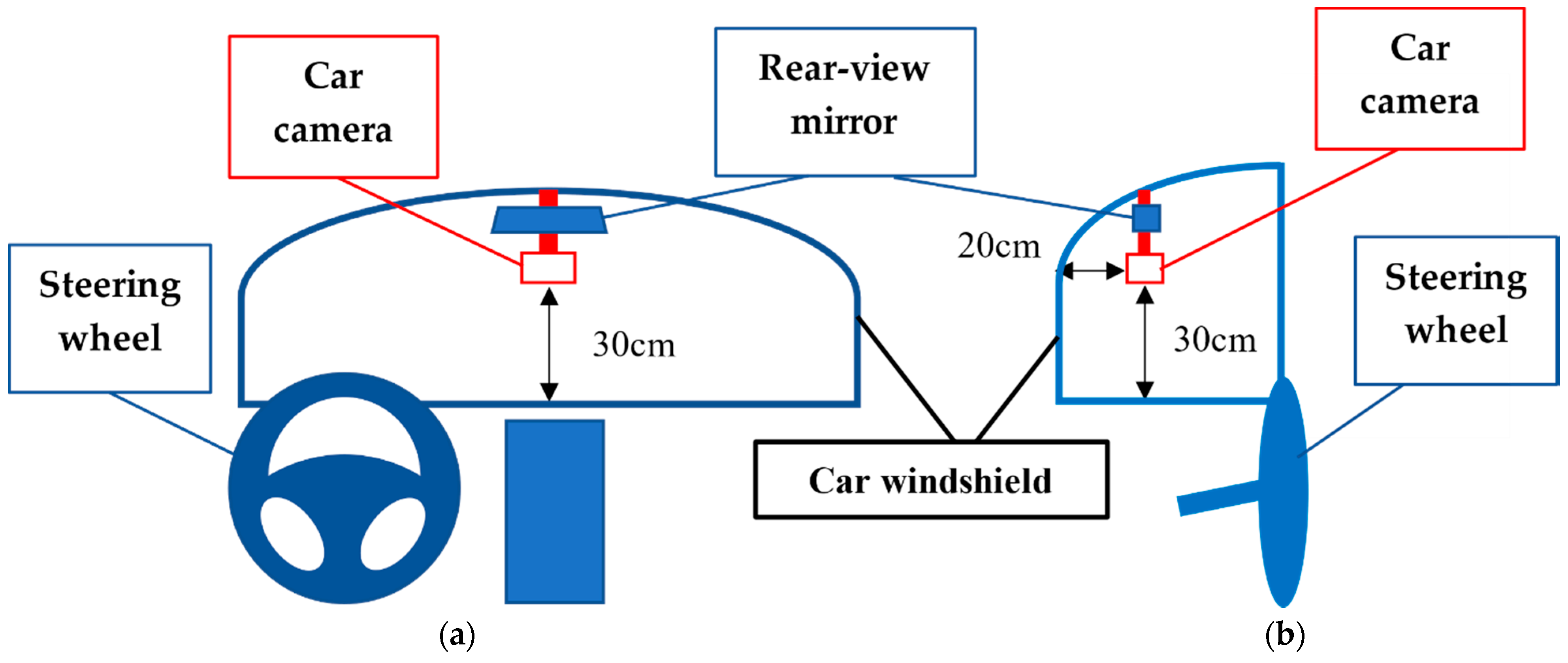
The view of the camera placed inside the vehicle is shown in Figure 9. Image (a) is the front view of the position of the camera inside the car, which was about 30 cm away from the steering wheel. The red rectangle is the car camera and the trapezoid above the car camera is the rear-view mirror. Image (b) is the side view of the position of the car camera inside the car, which is about 30 cm away from the steering wheel and 20 cm away from the car windshield.

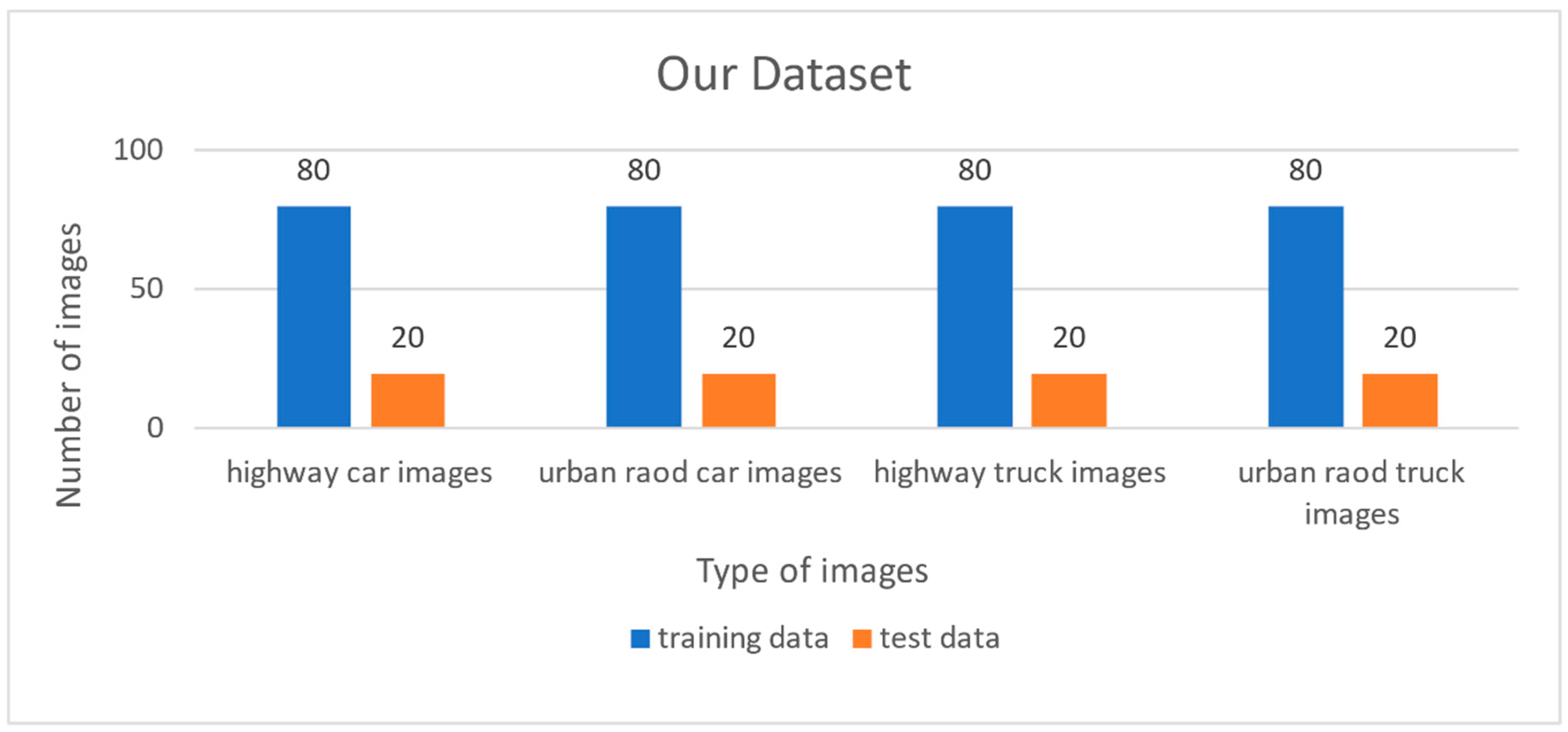
There were 400 road images in our data set, of which 320 images were training data and 80 images were test data. These images were collected from the car camera in the car when driving on the urban road and highway. There were four types of images in our data set, as shown in Figure 10. The blue bar is the training data while the orange one is the test data.

3.1.2. Car Object Detection Model Structure

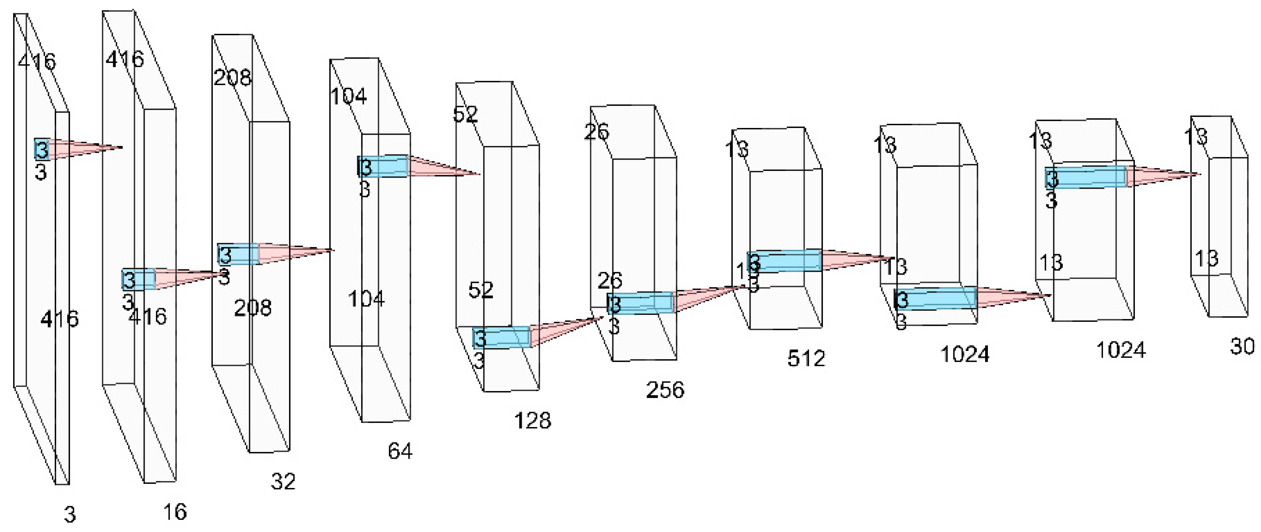
We used Darkflow [18], which is the github open source code. It is written in the Python background and designed as the YOLO version two. We applied a simpler version of the YOLOv2 model structure called Tiny YOLO VOC, which is a kind of object detection model, and we did not change any of the model’s parameters [18]. Figure 11 shows the structure of the Tiny YOLO VOC model and the essential parameters of Tiny YOLO VOC are shown in

Table 1. The parameters of tiny-YOLO-VOC structure.

Layers	Details	Output Size
1	Conv2d(filters = 16, kernel_size = 3, stride = 1, Batch_normalize = 1, Activation_function = Leaky Relu)	16 x 416 x 416
2	Maxpooling2d(pool_size = 2, stride = 2)	16 x 208 x 208
3	Conv2d(filters = 32, kernel_size = 3, stride = 1, Batch_normalize = 1, Activation_function = Leaky Relu)	32 x 208 x 208
4	Maxpooling2d(pool_size = 2, stride = 2)	32 x 104 x104
5	Conv2d(filters = 64, kernel_size = 3, stride = 1, Batch_normalize = 1, Activation_function = Leaky Relu)	64 x 104 x104
6	Maxpooling2d(pool_size = 2, stride = 2)	64 x 52 x 52
7	Conv2d(filters = 128, kernel_size = 3, stride=1, Batch_normalize = 1, Activation_function = Leaky Relu)	128 x 52 x 52
8	Maxpooling2d(pool_size = 2, stride = 2)	128 x 26 x 26
9	Conv2d(filters = 256, kernel_size = 3, stride = 1, Batch_normalize = 1, Activation_function = Leaky Relu)	256 x 26 x 26
10	Maxpooling2d(pool_size = 2, stride = 2)	256 x 13 x 13
11	Conv2d(filters = 512, kernel_size = 3, stride = 1, Batch_normalize = 1, Activation_function = Leaky Relu)	512 x 13 x 13
12	Maxpooling2d(pool_size = 2, stride = 1)	512 x 13 x 13
13	Conv2d(filters = 1024, kernel_size = 3, stride = 1, Batch_normalize = 1, Activation_function = Leaky Relu)	1024 x 13 x 13
14	Conv2d(filters = 1024, kernel_size = 3, stride = 1, Batch_normalize = 1, Activation_function = Leaky Relu)	1024 x 13 x 13
15	Conv2d(filters = 30, kernel_size = 1, stride = 1, Activation_function = Leaky Relu)	30 x 13 x 13

. The white rectangles are the layers, and the blue rectangles and red triangles are the sign of convolution process.

The model was designed as the YOLOv2 form, so there were no fully connected layers in the structure. The model contains nine convolutional layers. The input is 416 × 416 × 3 and the output is 13 × 13 × 30. When the road images are input, it goes through nine convolutional layers. Eight of them have the same parameters, including kernel_size of 3, stride of 1, Batch_normalize of 1, and activation_function of Leaky Relu. The parameters of the last convolutional layer include kernel_size as 1, stride as 1, and activation_function as Leaky Relu. The filters from the first convolutional layer to the last convolutional layer are 16, 32, 64, 128, 256, 512, 1024, 1024, and 30. For the meaning of the parameters in each convolutional layer, the filters mean the number of output filters in the convolution, kernel_size is the 2-D convolution window that slides the whole image, stride means the strides of the convolution along the height and width, Batch_normalize means the batch normalization, and activation is the activation function to use. At last, we set the filter number of the output layer at 30 due to there being only one class. The 30 count is obtained by adding one to five and then multiplying by five. One is class number, the first five refers to the values that the bounding box contains, while the latter five refers to the number of anchor boxes. This is our car detection model.

3.1.3. Training of Car Object Detection Model

As we obtained our training datasets and our model, we could commence with training. We used labelImg [19], which is also the github open source, to get the training label. The form of the training label was an xml file. Then, we trained our car object detection model three times. The model could learn to adjust its parameters in each step. At the first training, we had to pretrain our car object detection model. We used tiny-YOLO-VOC.weights [11], which is a pre-trained model developed by the authors of YOLO to pretrain our car detection model. The chief benefits are that it can make our model easy to learn and have better results. We set the learning rate to 0.001, batch size to 16, and epoch to 10, as shown in

Table 2. First training parameters of the car object detection model.

Parameters	Values
Number of epochs Batch size Learning rate Size of input image Input’s channels	10 16 0.001 416 3

. Secondly, we loaded our pretrained car object detection model to proceed with training. In the second training, the learning rate was modified from 0.001 to 0.00001, as written in

Table 3. Second training parameters of the car object detection model.

Parameters	Values
Number of epochs Batch size Learning rate Size of input image Input’s channels	10 16 0.00001 416 3

, and the other parameters remained the same. Lastly, our learning rate was 0.00001, and we revised the batch size to 8 and epoch to 25, as shown in

Table 4. Last training parameters of the car object detection model.

Parameters	Values
Number of epochs Batch size Learning rate Size of input image Input channels	25 8 0.00001 416 3

. Finally, we received our well-trained car detection model. The weight files were pb and meta, which are the common form of tensorflow weights. This was the process of our car detection model training.

3.2. Lane Line Detection

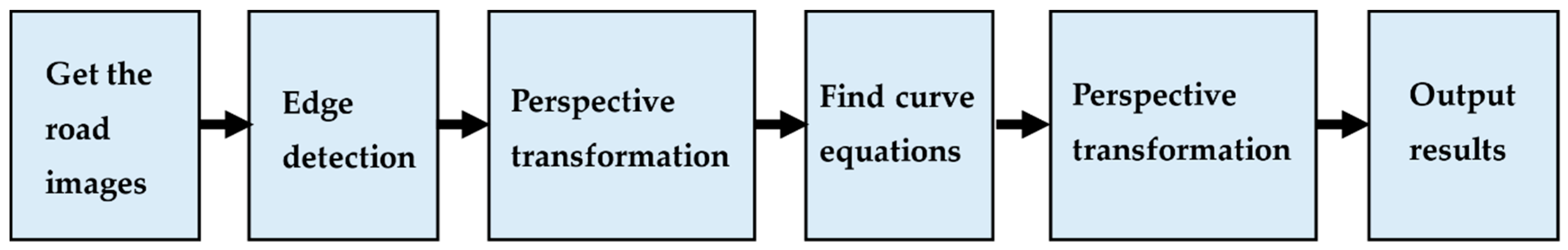
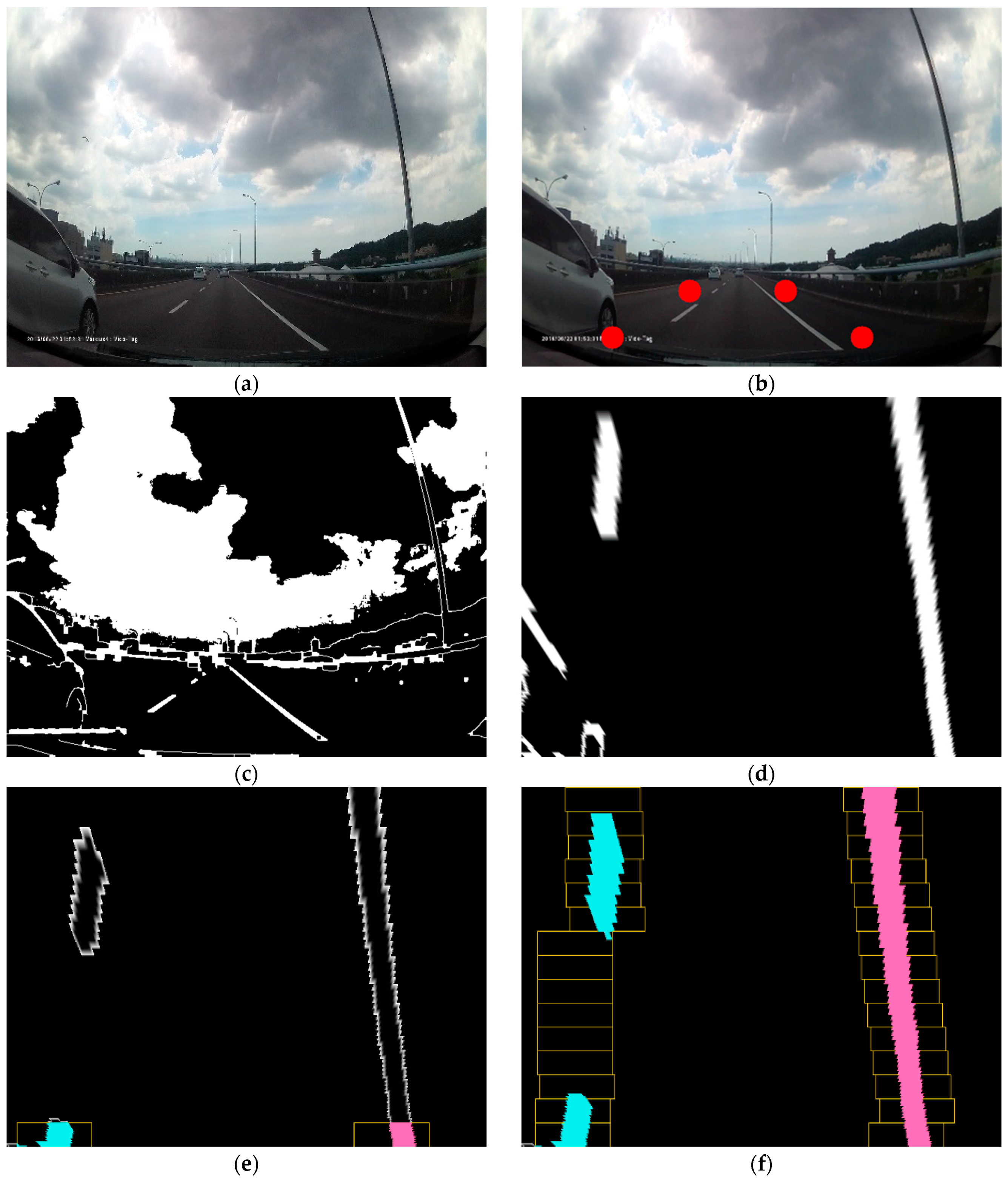
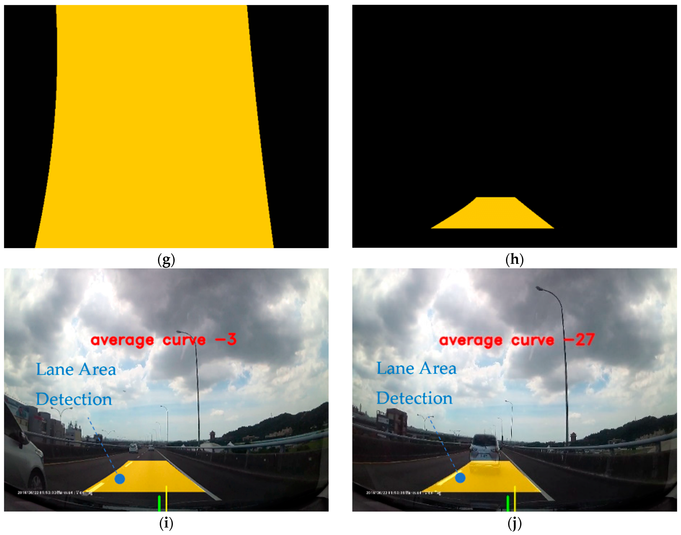
The lane line detection system can detect the lane line area on the road, assisting the drivers to drive in the appropriate lane. In this part, we discuss the process of lane line detection. The flow-charts of lane line detection are shown in Figure 12. When the road images were input, the edge detection was used to obtain the edged image. Next, perspective transformation was applied to convert the 3-D view to the 2-D view, and we could find the curve equations of lane lines. After obtaining the equations, we drew the lane area and performed the perspective transformation again. Finally, we could obtain the lane region and complete lane line detection.

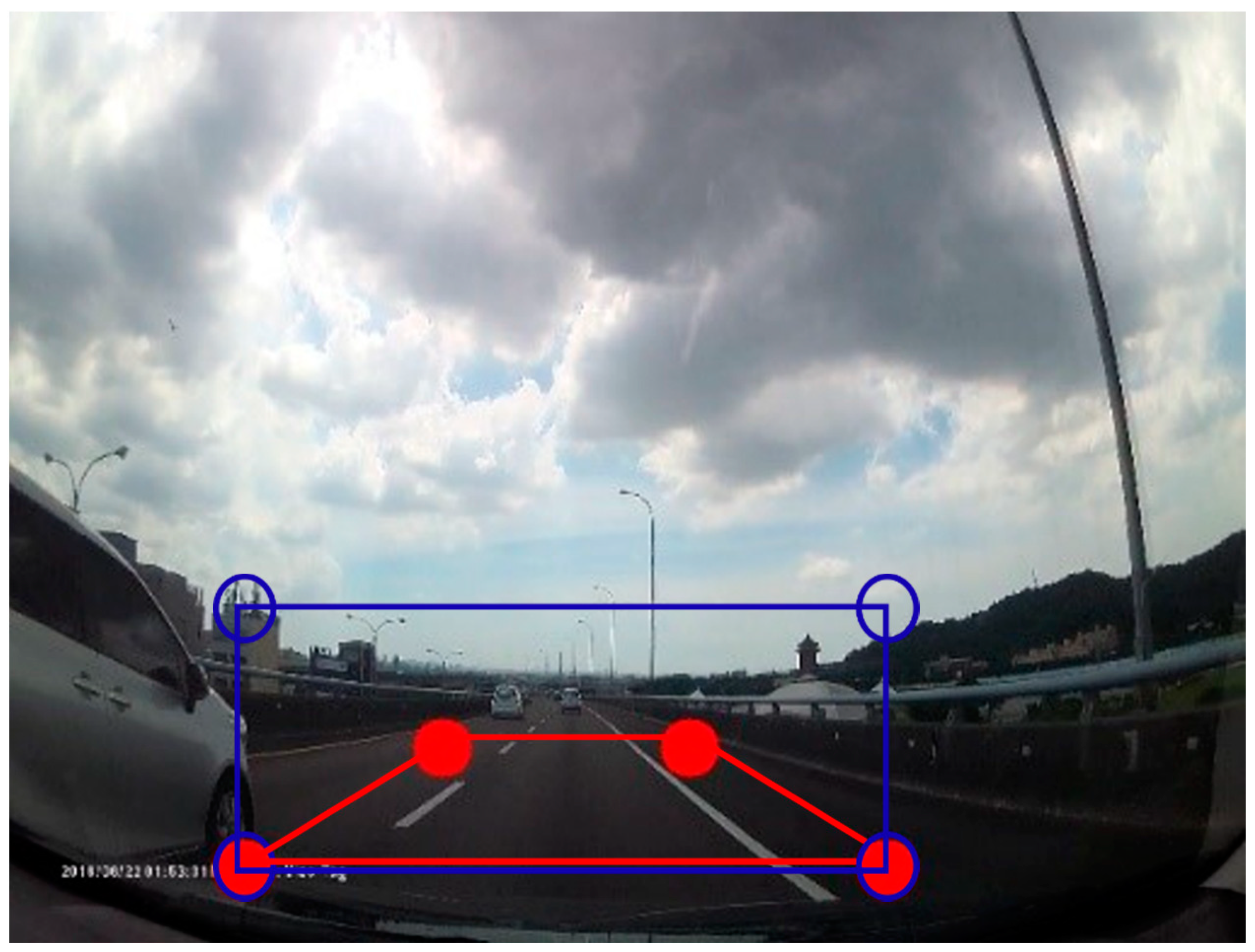
Our input images were ground truth images from the car recorder. After image input, we needed to find eight points on it (Figure 13). The red points could generate an area, which covered the two road lines. These eight points were later used in the process of the projection transformation.

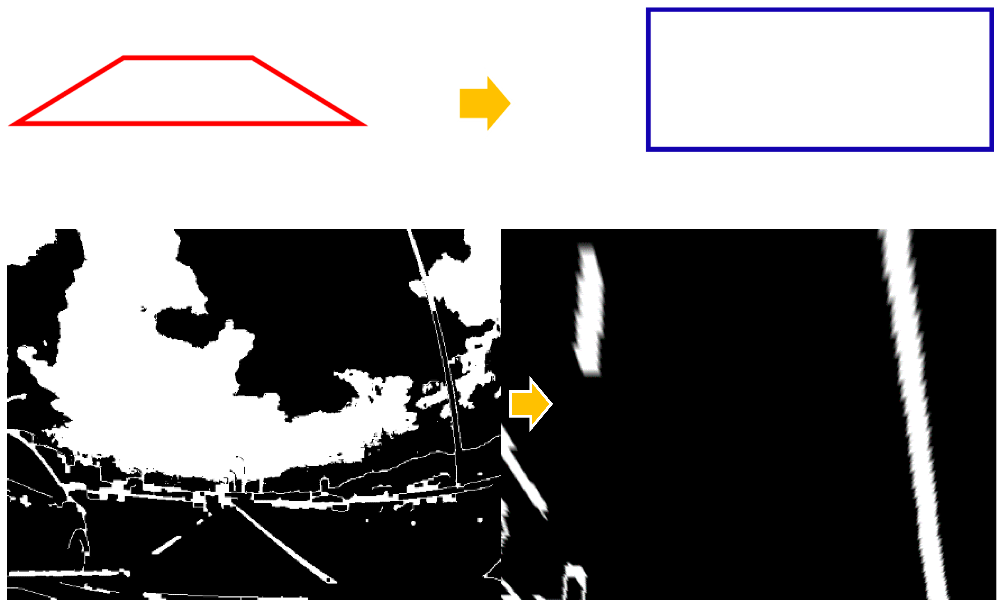
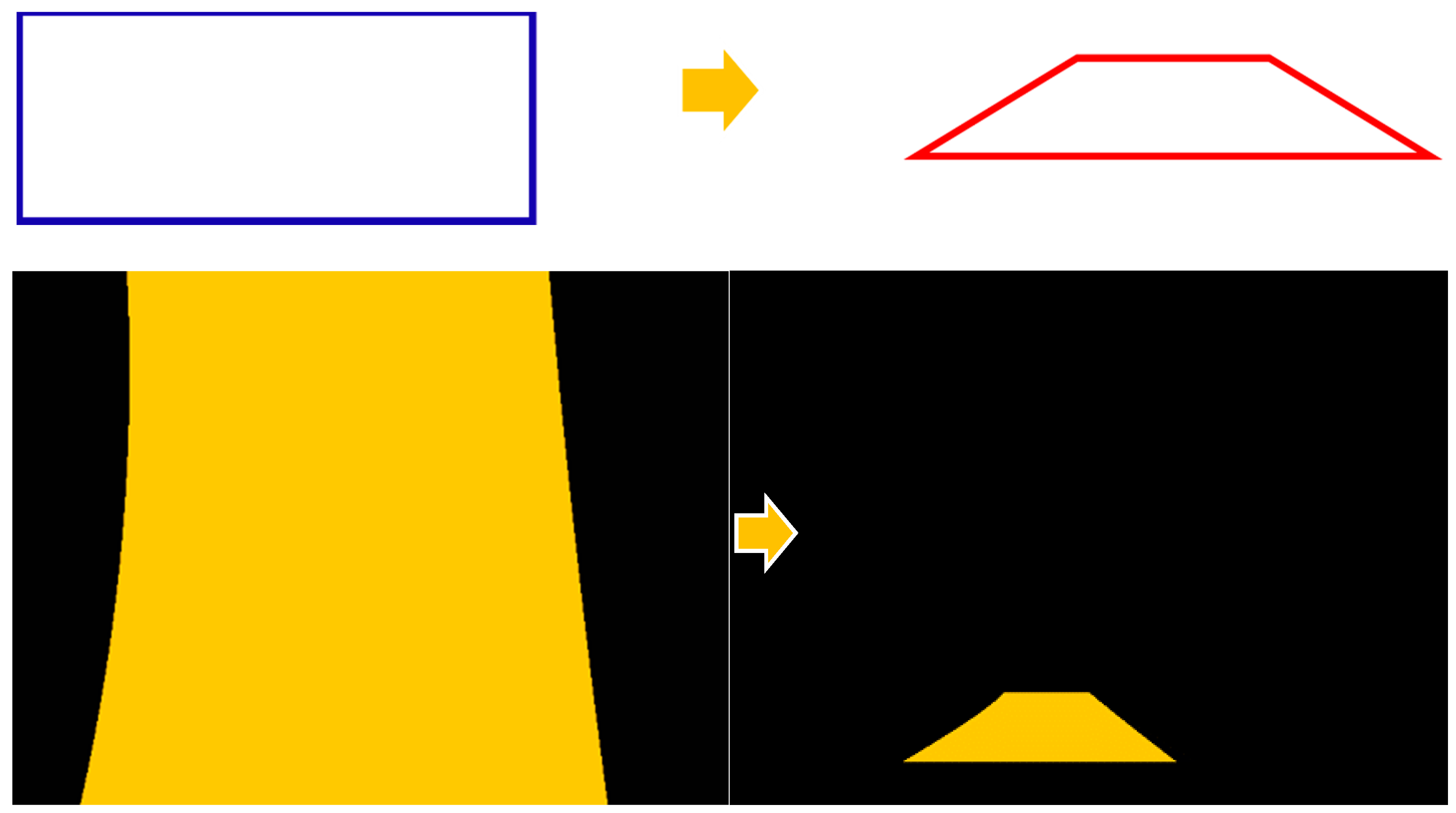
In order to obtain clear road lines, edge detection was carried out on our input road images. We used the projection transform to obtain the edged road images. This was the most significant step in the lane line detection. The main purpose of it was to convert the perspective from the 3-D view to the 2-D view, as seen in Figure 14. We conducted projection transformation twice in the lane line detection. Furthermore, the images of the projection transformation were used to find the curve equation that fit the two road lines. After obtaining the curve equations, we plotted our lane area. Since we processed the projection transformation, we had to convert the lane area from the 2-D view back to the 3-D view. Figure 15 shows the projection transformation of the lane area. In the end, we could combine the lane area with the original road image. The above is the entire process of lane line detection.

3.3. Trajectory Prediction of a Car

This section is the substantive content of our research. We sequentially discuss our data set, our car trajectory prediction model structure, and the training of the model. Our process is shown in the following sections. A flow-chart of the trajectory prediction of a car is shown in Figure 16. After the road images were input, object detection of the car was applied to obtain the X and Y coordinates of the car in the images. In addition, we built training data, which contained X and Y coordinates of the car and the training label, containing only the X or Y coordinates of the car. Next, we built and trained a trajectory prediction model based on LSTM. Finally, we tested and evaluated the model.

3.3.1. Data Set

We used the same data set in Section 3.1.1, and the technique in Section 3.1 was applied as well. We made use of car object detection to detect the car in the road image. It simultaneously obtained the car coordinates, representing the car location in the image. We could gather these coordinate changes over times, and they could become a certain car’s trajectory. Finally, these coordinates were saved in an Excel file, as shown in

Table 5. X and Y coordinates of the car saved in an Excel file.

1	X	Y
2	4.999238	0.174524
3	5.04951	0.178052
4	5.099782	0.181615
5	5.150053	0.185213
6	5.200325	0.188846
7	5.250597	0.192515
8	5.300869	0.196219
9	5.35114	0.199959
10	5.401412	0.203733
11	5.451684	0.207543
12	5.501955	0.211389
13	5.552227	0.215269
14	5.602499	0.219185
15	5.65277	0.223136
…	…	…

. The x and y contained in the Excel file referred to the x coordinates and y coordinates of the car in the road image.

3.3.2. The Structure of the Car Trajectory Prediction Model

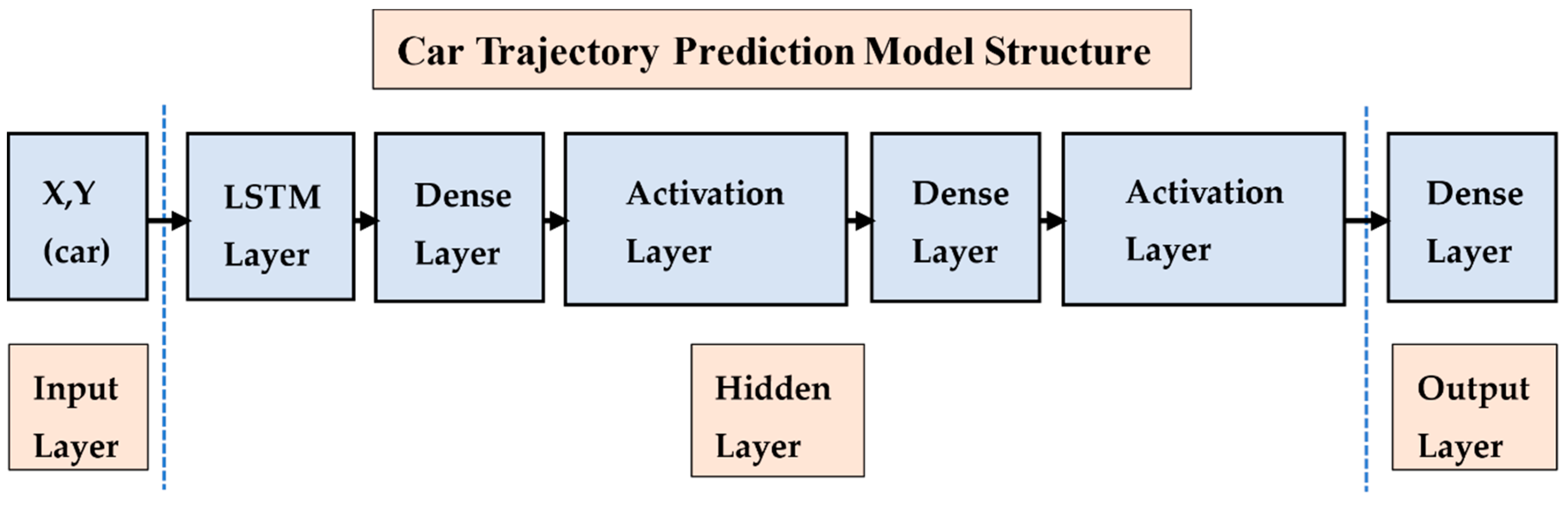
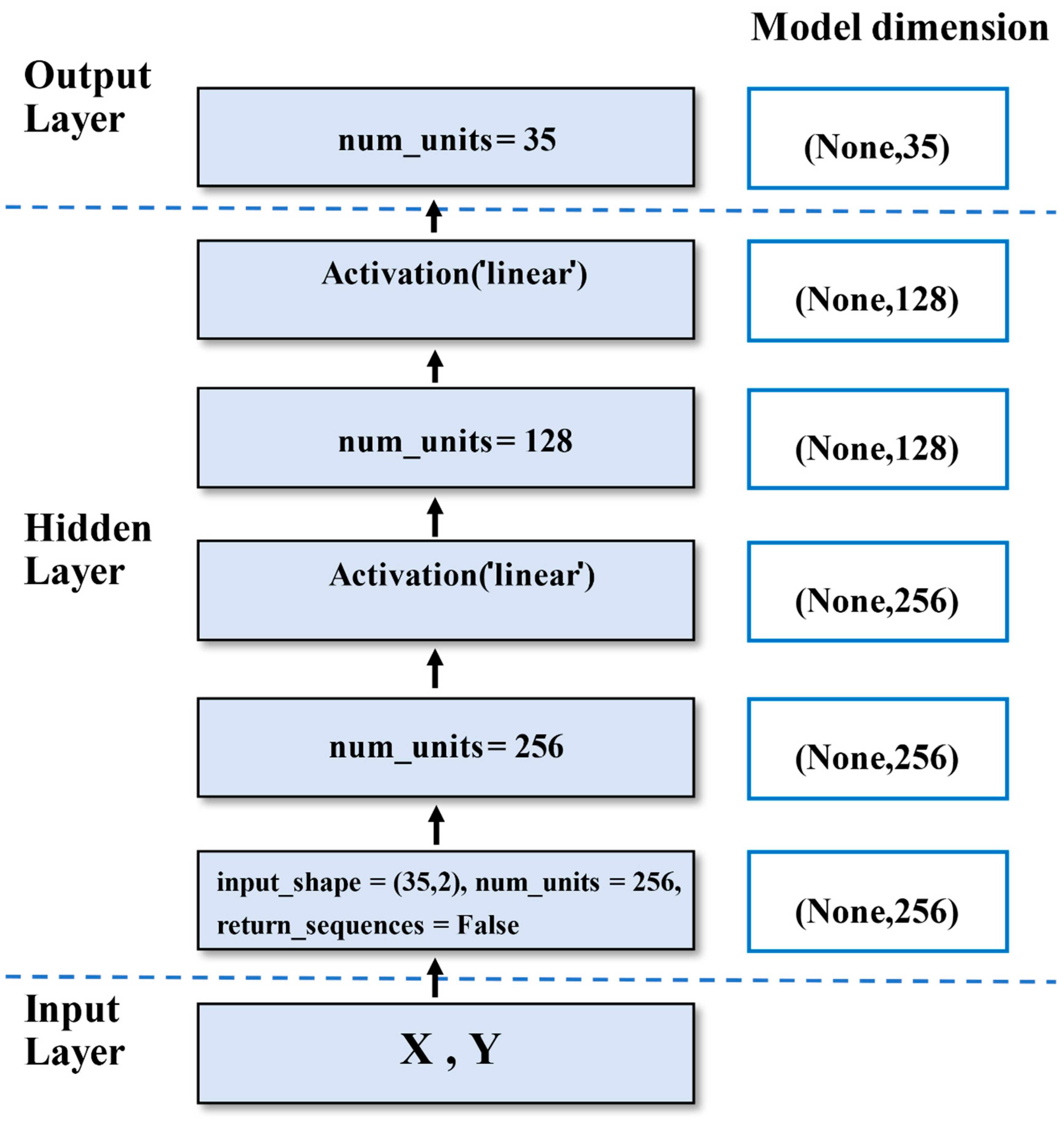
We used LSTM to construct our car trajectory prediction model based on keras in the Python background. Figure 17 shows our model structure. There were six layers, including one LSTM layer, two activation layers, and three dense layers. The first was input layer, and the X and Y coordinates of the cars were the input to the input layer. Next was the LSTM layer. We set the unit number at 256, input shape as (35,2), and return sequences as False. Our activation function was selected to be linear. In addition, we set the number of units in each dense layer to 256, 128, and 35. The essential parameters of the car trajectory prediction model are shown in

Table 6. The parameters of the car trajectory prediction model structure.

Layers	Details	Output Size
1 2 3 4 5 6	LSTM(num_units = 256, input_shape = (35,2), return_sequences = False) Dense(num_units = 256) Activation(‘linear’) Dense(num_units = 128) Activation(‘linear’) Dense(num_units = 35)	(None, 256) (None, 256) (None, 256) (None, 128) (None, 128) (None, 35)

. In the LSTM layer, num_units referred to the number of hidden units, input_shape the input shape, and return_sequences indicated whether to return a single hidden state value or the hidden state value of all time steps. False returns were single, and true returns were all. In the Dense layer, num_units represented the number of hidden units. Activation was the activation function to be used, and we used the linear function. In the output layer, it only contained the X or Y coordinates of the cars because we trained the model to predict X and Y separately. The detailed parameter diagram of the model is presented in Figure A1 in the Appendix A.

3.3.3. The Training of the Car Trajectory Prediction Model

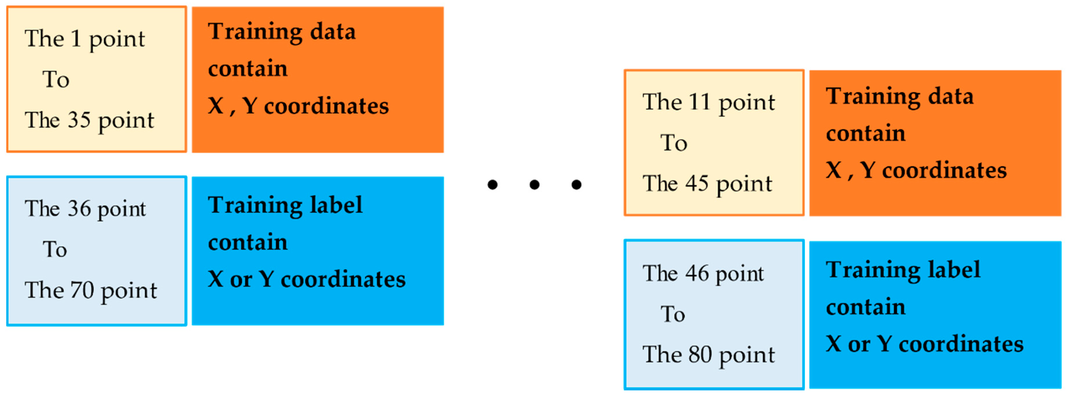
In the training process, we required certain model training data. We used the data set from Section 3.3.1. Next, the training data and train label could be constructed. Our aim was to train the model to predict the future trajectory of the car. Points 1 to 35 were used to predict the next 35 points. Figure 18 shows the method used to obtain the training data and labels.

Thus, we set points 1 to 35 as our first training data, and points 36 to 70 as our training labels. The training data had two columns, X and Y, which were the x coordinates and y coordinates of the car location in the road image. We decided to train the model to predict x and y coordinates separately. Thus, the training label contained only x coordinates or y coordinates. It is worth nothing that training labeling was significant in the training process. The training label can decide the model used to predict which features. For instance, if we want the model to predict future x coordinates of the car, the only thing we need to do is set the training label as x coordinates of the car. Furthermore, the model will learn to predict future x coordinates of the car. Thus, if we set the training label as y coordinates of the car, the model will learn to predict future y coordinates of the car.

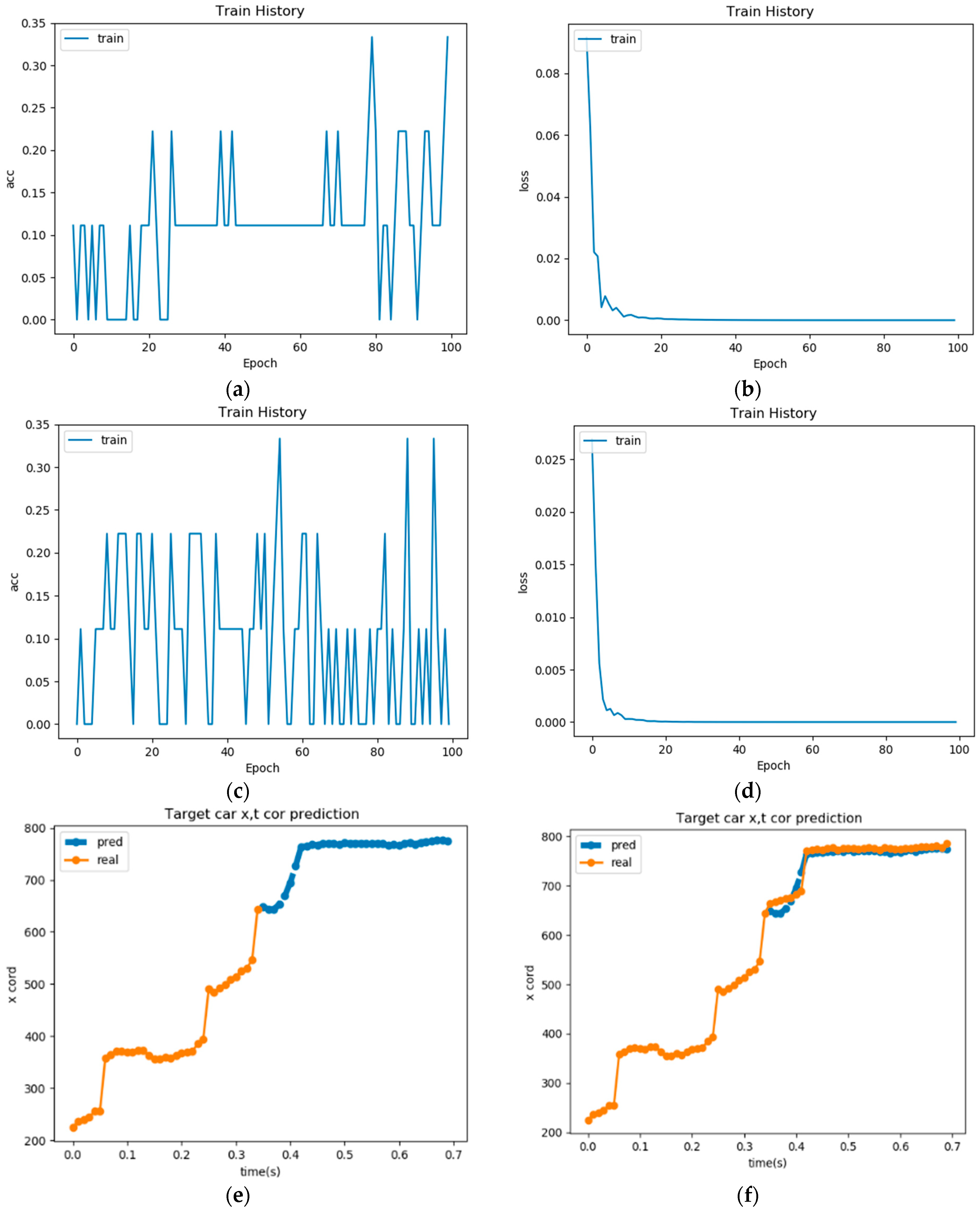
After obtaining the training data, training label, and our car trajectory prediction model, we had to set up the training parameters. We set the epochs as 100 times and batch size as 5. Loss function was mean square error (MSE), and the optimizer was Adam. The essential parameters of the car trajectory prediction model are shown in

Table 7. Training parameters of the car trajectory prediction model.

Parameters	Values
Number of epochs Batch size Learning rate Input shape Loss function Optimizer	100 5 0.001 (35,2) MSE Adam

.

3.4. Combination

We combined the techniques from Section 3.1, Section 3.2 and Section 3.3. We combined all Python code together. When the road images were input, it could process car detection, lane line detection, and car trajectory prediction simultaneously. As a result of the input of the three techniques was road image so that we could achieve this combination. Figure 19 shows our concept of the combination of techniques.

4. Results and Discussion

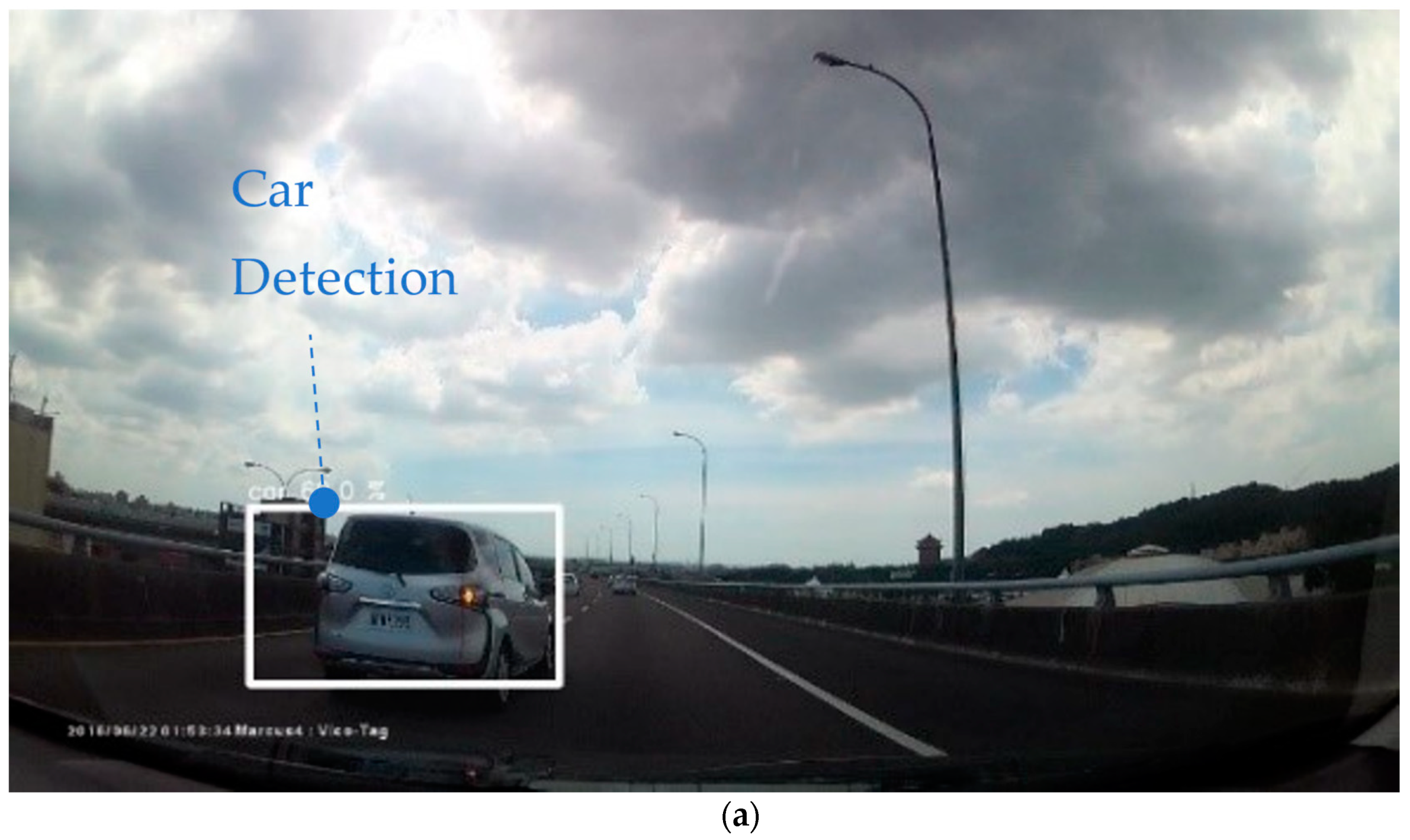
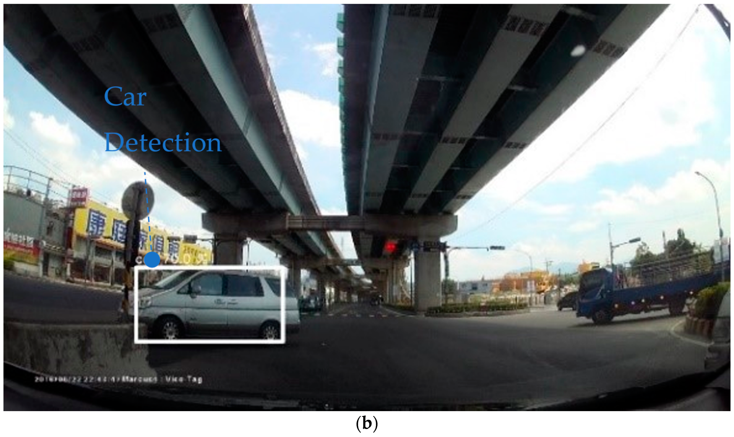
In this section, we show our research results and discuss them. The first is car object detection, the results of which are shown in Figure 20a,b. We find that the model is quite accurate. It has the ability to detect the car precisely. In the first training, it took 5 min and 58 s to train the car detection model. The loss dropped from 106.00877 to 0.96654, and the average loss from 106.00877 to 3.2454. At the second training step, it took 5 min and 57 s to train. The loss and the average loss fell to 0.69618 and 0.83406, respectively. Finally, in terms of the training step, because training was carried out 25 times, it took 15 min and 10 s. Fortunately, the loss and the average loss dropped to 0.22245 and 0.39897, respectively. The training results of car object detection are demonstrated in

Table 8. The training results of the car detection model.

Training Step	Training Time	Loss		Average Loss
		Max	Min	Max	Min
1	5 min 58 s	106.00877	0.96654	106.00877	3.2454
2	5 min 57 s	1.05844	0.69618	0.98139	0.83406
3	15 min 10 s	1.06956	0.22245	0.80912	0.39897

, and the evaluation results of the images of the trained car detection model are shown in

Table 9. The evaluation results of images of the car detection model.

Test Image Number	Total Processing Time (s)	Accuracy
1–10	0.3637	0.75
11–40	0.9518	0.86
50	0.132	0.71
65	0.159	0.89

. In the evaluation, the accuracy reached 0.89, and it only took 0.132 s to detect the car. Furthermore, the evaluation results of videos of the trained car detection model are shown in

Table 10. The evaluation results of videos of the car detection model.

Time in Video (s)	FPS		Accuracy
	Max	Min	Max	Min
1–5 s	10.995	10.868	0.88	0.72
5–10 s	10.202	9.461	0.91	0.76

. We used the value of frame per second (FPS) to measure the smooth performance of a video. The larger the number of FPS, the faster the display speed, the higher the frequency, and the smoother the image. The model was detected at 10.995 FPS, with an accuracy of 0.91, which is close to real time detection.

Secondly, we conducted lane line detection. Figure 16 shows the entire process of lane line detection. In lane line detection, we did not utilize the deep learning framework to construct neural networks but instead used OpenCV [14], which is a tool to process computer vision, to conduct our lane line detection process.

Despite the fact that we did not apply deep learning, we found that our lane detection results were quite good, as seen in Figure 21. It could genuinely detect the lane line and draw the appropriate lane area. This is a promising result because we can now use lane area to deal with other valuable issues. For example, we can use lane area to build a warning system, which can draw the driver’s attention to decelerate preventively and drive safely in the appropriate lane.

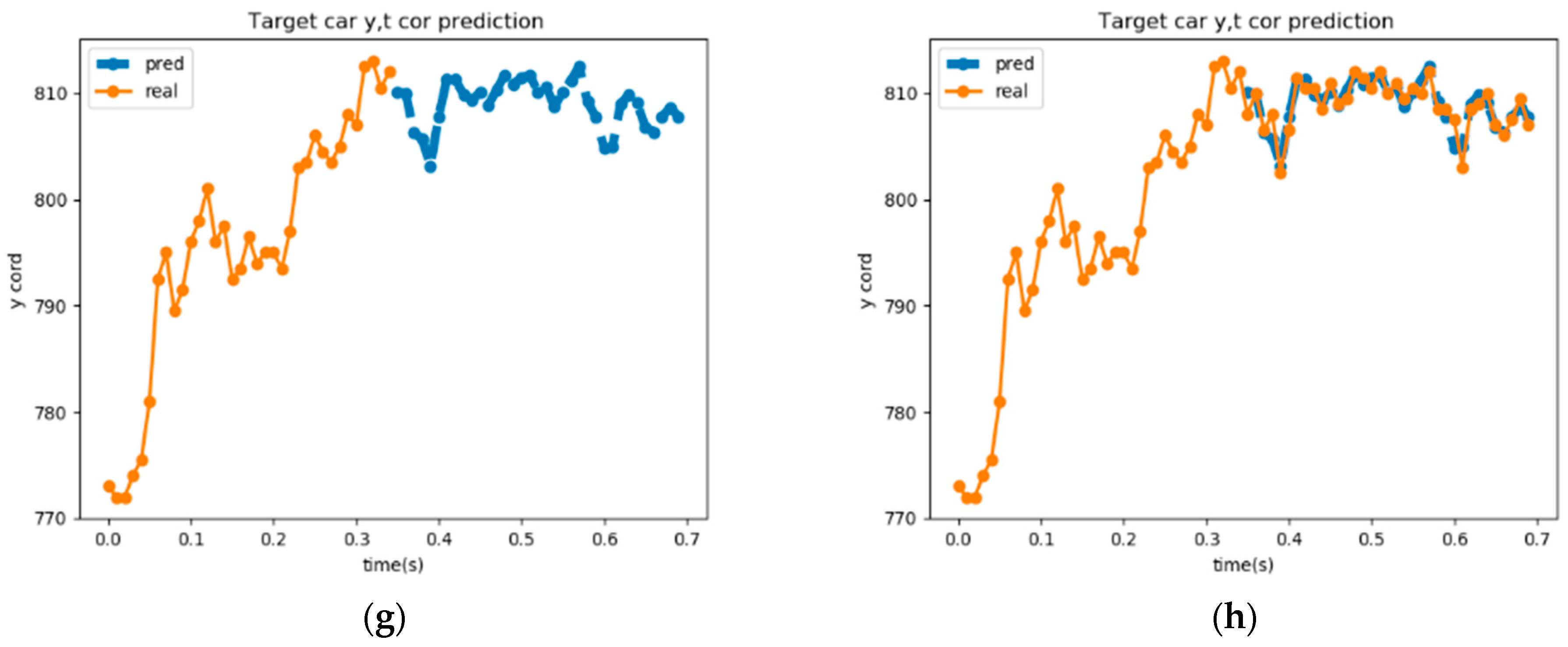
Next, we showed our training for the car trajectory prediction (Figure 22). We constructed two models, which are the model that predicts future x coordinates of the car and the model that predicts future y coordinates of the car. We trained these two models separately. Thus, our training data were the same, while the training label was different. One contained x coordinates, and the other contained y coordinates. It took 6.829 s to train the x model and 6.75986 s to train the y model. The regression metrics were used to train our model, and we hoped that the predicted value as close to the actual value as possible. In addition, we used mean squared error (MSE) as our loss function. Thus, if the predicted value is close to the actual value, the loss will be small, and the accuracy will be high. If the accuracy is 1, this means that the predicted value is exactly the same as the actual value. However, this is quite difficult to achieve. In the evaluation, we used a trained model to predict the trajectory, which was not in the data set. We found that the model learned quickly, and the loss descended rapidly from 0.07694 to 0.00017 for the x model and 0.02107 to 0.00098 for the y model. However, the training accuracy was very poor. Surprisingly, although the accuracy was quite low, both x and y model could predict accurately when we verified the model. In addition, the processing time was only 12 milliseconds, and the losses were 0.000248 for the x model and 0.000932 for the y model. The training results of the x and y coordinates of the car trajectory model are demonstrated in

Table 11. The training results of car trajectory prediction model.

Model	Training Time (s)	Accuracy		Loss		Evaluation Time (ms)	Evaluation Score
		Max	Min	Max	Min		Acc	Loss
Predict X coordinates	6.829	0.33396	0.00104	0.07694	0.00017	12	0.22222	0.000248
Predict Y coordinates	6.75986	0.33357	0.00054	0.02107	0.00098	12	0.11111	0.000932

, which contains the processing time and score value of evaluation.

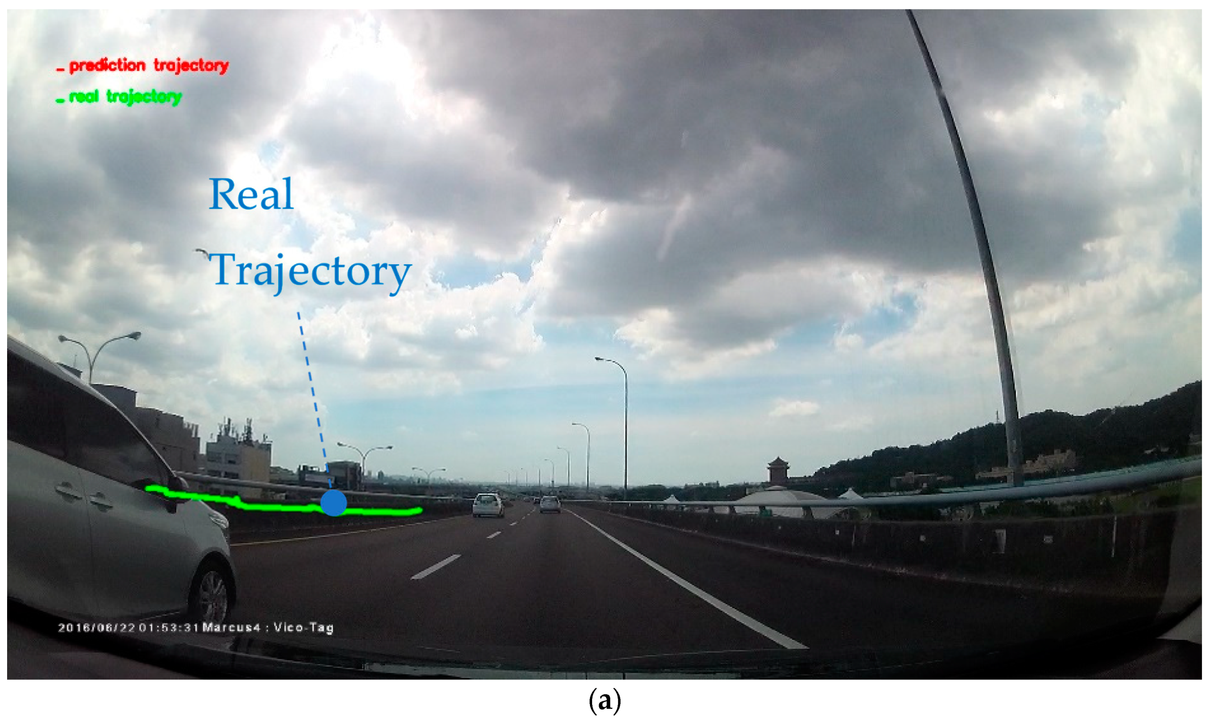
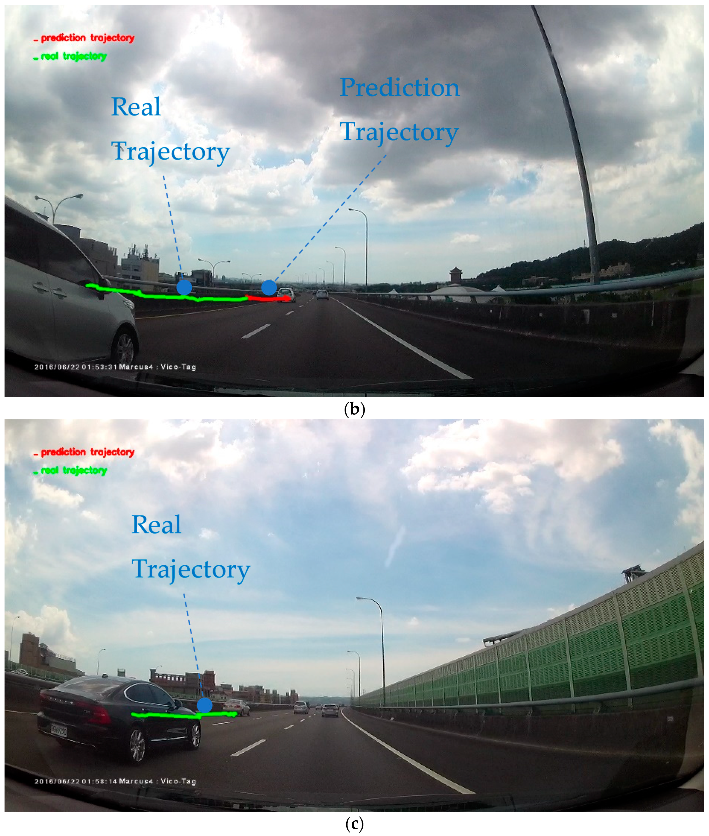
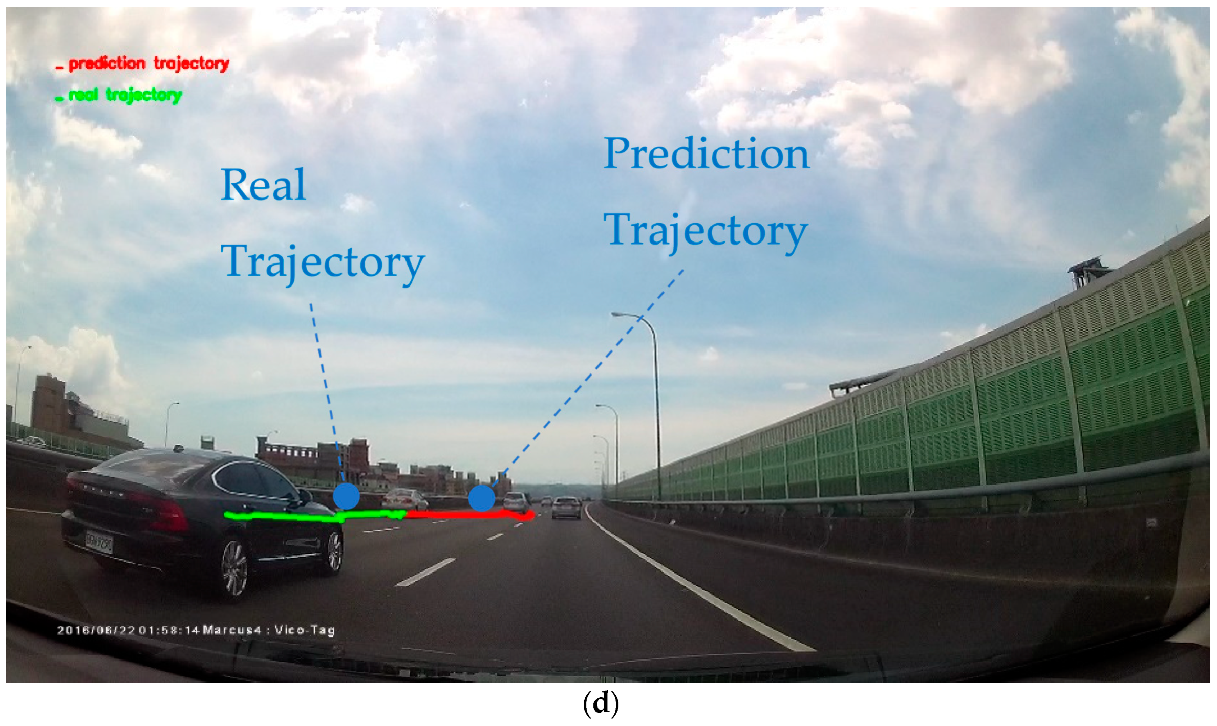
The car trajectory prediction results are shown in Figure 23. The ground truth road images were used to be our input. Then, we used car object detection first, and applied car trajectory prediction. We found that the car trajectory model had the ability to predict the future trajectory quite well, as seen in in Figure 18.

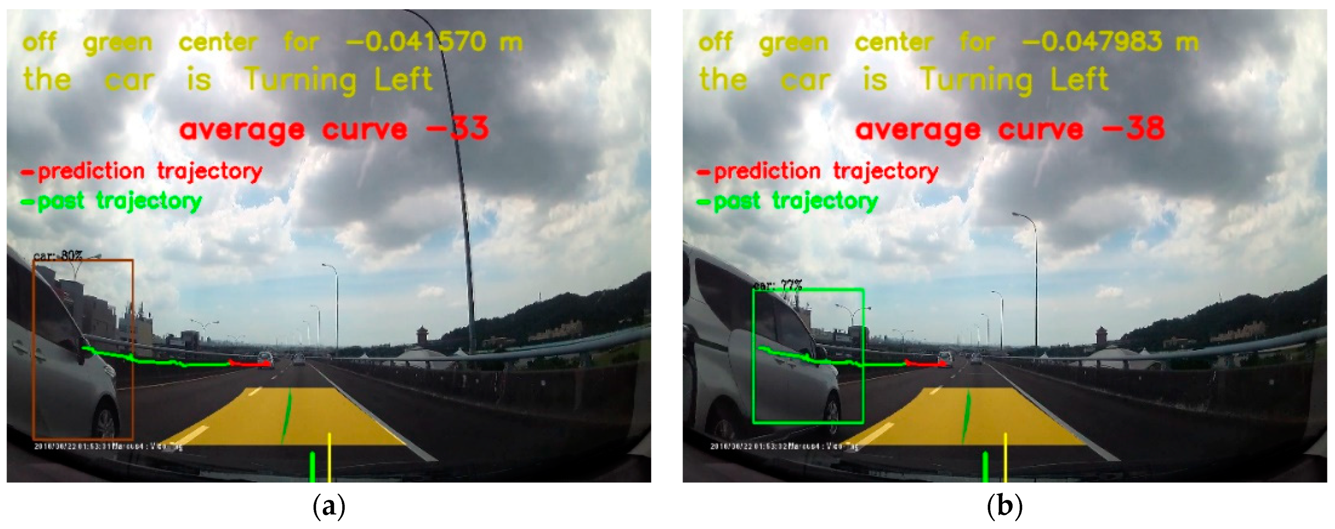
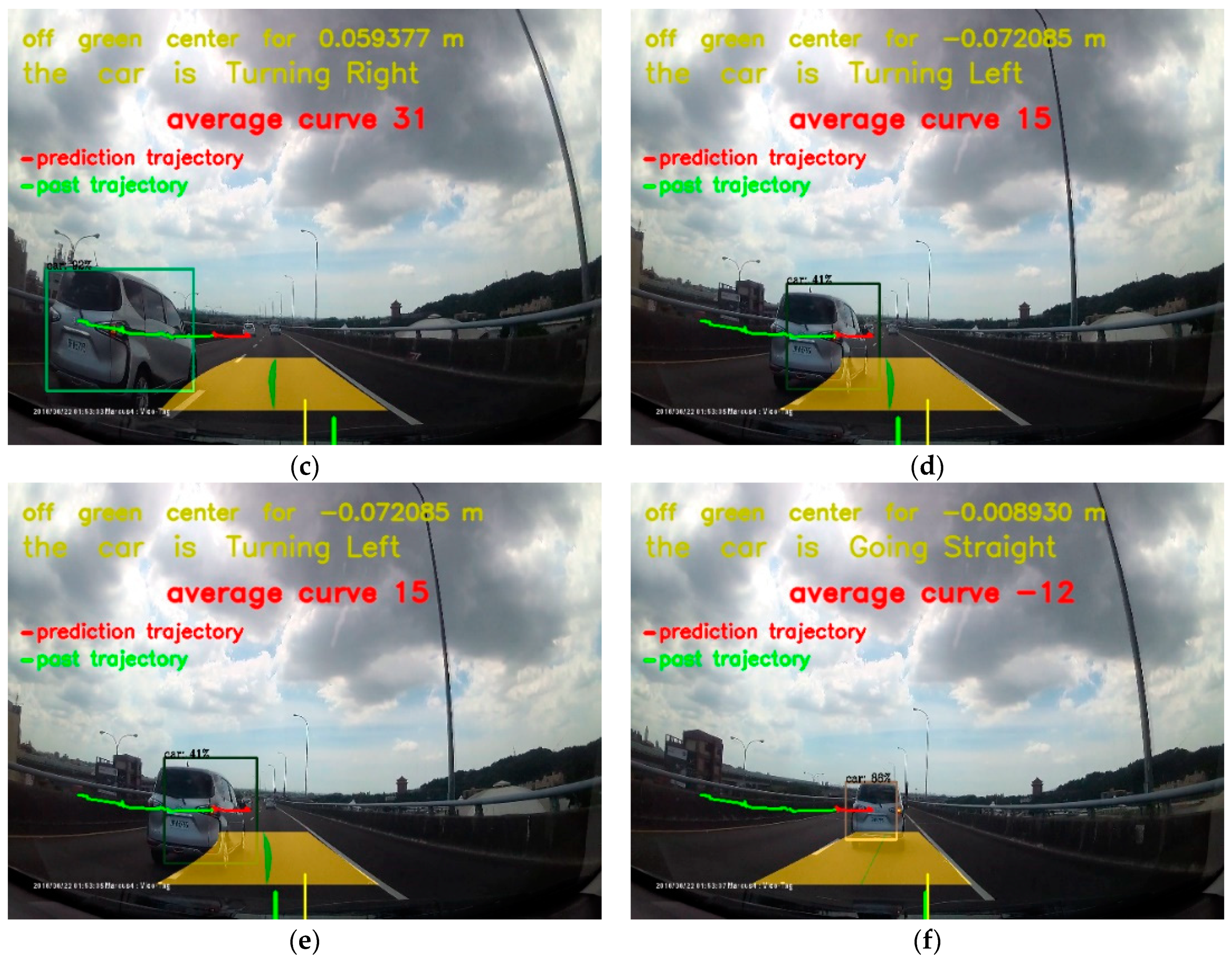
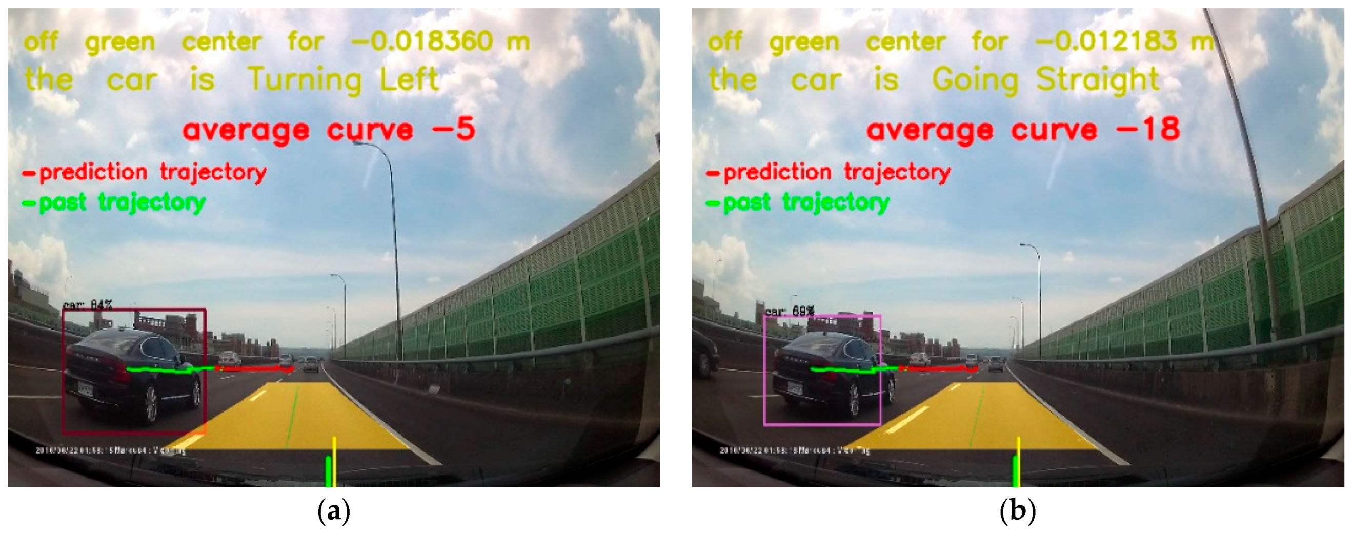
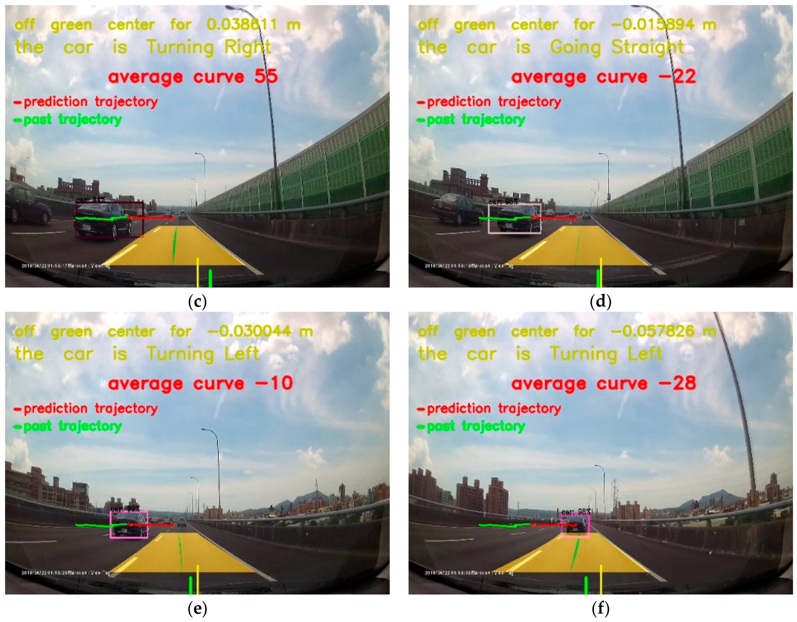
At last, we showed the results of the combination of all techniques. Figure 24 shows the first results of the validation. All the images in Figure 24 show the three techniques, namely car object detection, lane line detection, and car trajectory prediction. The images (a), (b), and (f) in Figure 24 show excellent results. However, as seen in images (c), (d), and (e) in Figure 24, while the car detection and car trajectory prediction performed quite well, unfortunately, we found that the lane area in these three pictures was slightly wrong due to other vehicles blocking our lane line. In image (d), the car on our left side crossed the lane so as to block the lane line. It caused the process of lane line detection to obtain the wrong curve equation. That is to say, the detection of the lane area was wrong. We considered that to be reasonable. If other vehicles were to cross the lane, we definitely would not be able to see the lane line as well due to the lane line being blocked by others.

Figure 25 shows the three techniques used, including car object detection, lane line detection, and car trajectory prediction.

We could assume that there were two crucial factors that would affect the lane detec-tion based on the results shown in Figure 24 and Figure 25. First of all, when one of our lane lines would be blocked by other cars, the detection of the lane area would be wrong. Sec-ondly, if the car in front of us would be very close to us, the lane area detection would likewise be wrong.

The proposed system must achieve the promised results of driver safety, which include object detection of the car, lane line detection, and trajectory prediction of the car, and the system needs to detect at each frame. The object detection and trajectory prediction of the car must not be affected by other cars crossing the lane line and they must detect efficiently. In lane line detection, two lane lines are required to find curve equations. Thus, the equations cannot be found if a vehicle crosses the line at a certain frame. Moreover, we are not capable of seeing the line blocked by the vehicle as well when we are sitting in the driver’s seat. If the two lines are not blocked by vehicles, we can obtain good lane line detection results. It is when a vehicle is crossing the lane line and is very close to us that our lane area will be affected. Although the vehicle crossing the line may influence the lane line detection, such as deformation of the lane area, it can still warn the drivers to slow down or take other measures. In addition, object detection and trajectory prediction of the car can help to remind the drivers as well. Therefore, based on the combination of multiple models to warn the drivers and enhance driving safety, our results are still promising.

Research Prospect

We look forward to proceeding with our research in three areas. First, the latest version of YOLO, such as YOLOv4 or YOLOv5, will be used. They not only have higher accuracy, but take less time to train the model, and require little time to detect objects. Next, we will use machine learning frameworks to construct the deep neural networks. We may use convolutional layers to address the images of computer vision. Lastly, the x and y coordinates of the car are predicted separately in this research. Therefore, we will make an effort to train the model to predict multiple features at the same time. In addition, the velocity and acceleration of the car will be added as our training features. We hope that we are capable of producing a more efficient and precise model. What is more, we will build a system that can warn the drivers. When other vehicles enter our lane area, or their predicted trajectory will cross the driver’s path, the system can warn the drivers to take the necessary measures. It can not only predict, but also issue warnings. It is a combination of all our work and also enhances driving safety.

5. Conclusions

The motivation of this research is to improve the safety of drivers. Car detection, lane line detection, and car trajectory prediction are applied to construct our warning system. Car detection has the ability to detect cars precisely, reaching an accuracy as high as 0.91 and taking merely 0.132 s to detect. Lane line detection can detect the appropriate lane area, which assists drivers to drive more safely. Car trajectory prediction, receiving a loss of 0.00024 and taking only 12 milliseconds to predict, is capable of predicting the future trajectory accurately and warning drivers to be more cautious and reduce the speed of the car in advance. By means of the above methods, based on the results of the two verifications, the probability of vehicle accidents can be reduced, and the safety of driving can be increased.

References

- Thompson, S.; Horiuchi, T.; Kagami, S. A probabilistic model of human motion and navigation intent for mobile robot path planning. In Proceedings of the IEEE Xplore, 2009 4th International Conference on Autonomous Robots and Agents, Wellington, New Zealand, 10–12 February 2009; pp. 663–668. [Google Scholar] [CrossRef]
- Alahi, A.; Goel, K.; Ramanathan, V.; Robicquet, A.; Fei-Fei, L.; Savarese, S. Social LSTM: Human Trajectory Prediction in Crowded Spaces. In Proceedings of the 2016 IEEE Conference on Computer Vision and Pattern Recognition (CVPR), Las Vegas, NV, USA, 26 June–1 July 2016; pp. 961–971. [Google Scholar] [CrossRef] [Green Version]
- Tharindu, F.; Simon, D.; Sridha, S.; Clinton, F. Soft + Hardwired attention: An LSTM framework for human trajectory prediction and abnormal event detection. Neural Netw. 2018, 108, 466–478. [Google Scholar] [CrossRef] [Green Version]
- Mikolov, T.; Karafiát, M.; Burget, L.; Cernocký, J.; Khudanpur, S. Recurrent neural network based language model. In Proceedings of the 11th Annual Conference of the International Speech Communication Association, INTERSPEECH 2010, Chiba, Japan, 26–30 September 2010. [Google Scholar]
- Hochreiter, S.; Schmidhuber, J. Long short-term memory. Neural Comput. 1997, 9, 1735–1780. [Google Scholar] [CrossRef] [PubMed]
- Altché, F.; de La Fortelle, A. An LSTM network for highway trajectory prediction. In Proceedings of the 2017 IEEE 20th International Conference on Intelligent Transportation Systems (ITSC), Yokohama, Japan, 16–19 October 2017; pp. 353–359. [Google Scholar] [CrossRef] [Green Version]
- Kuo, S. LSTM-Based Vehicle Trajectory Prediction. Master’s Thesis, Institute of Communication Engineering, National Tsinghua University, Hsinchu, Taiwan, 2018. Available online: https://hdl.handle.net/11296/q7qwdc (accessed on 20 August 2020).
- Park, S.H.; Kim, B.; Kang, C.M.; Chung, C.C.; Choi, J.W. Sequence-to-Sequence Prediction of Vehicle Trajectory via LSTM Encoder-Decoder Architecture. In Proceedings of the 2018 IEEE Intelligent Vehicles Symposium (IV), Changshu, China, 26–30 June 2018; pp. 1672–1678. [Google Scholar] [CrossRef] [Green Version]
- Leibe, B.; Schindler, K.; Cornelis, N.; Van Gool, L. Coupled Object Detection and Tracking from Static Cameras and Moving Vehicles. IEEE Trans. Pattern Anal. Mach. Intell. 2008, 30, 1683–1698. [Google Scholar] [CrossRef] [PubMed] [Green Version]
- Redmon, J.; Divvala, S.; Girshick, R.; Farhadi, A. You Only Look Once: Unified, Real-Time Object Detection. 2016. Available online: http://pjreddie.com/darknet/yolov1/ (accessed on 5 July 2020).
- Redmon, J.; Farhadi, A. YOLO9000: Better, Faster, Stronger. arXiv 2016, arXiv:1612.08242. Available online: http://pjreddie.com/darknet/yolov2/ (accessed on 5 July 2020).
- Qiu, D.; Weng, M.; Yang, H.; Yu, W.; Liu, K. Research on Lane Line Detection Method Based on Improved Hough Transform. In Proceedings of the 2019 Chinese Control And Decision Conference (CCDC), Nanchang, China, 3–5 June 2019; pp. 5686–5690. [Google Scholar] [CrossRef]
- Qin, Z.; Wang, H.; Li, X. Ultra Fast Structure-aware Deep Lane Detection. In Proceedings of the European Conference on Computer Vision (ECCV), Glasgow, UK, 23–28 August 2020. [Google Scholar]
- Bradski, G. The OpenCV Library. Dr. Dobbs J. Softw. Tools. 2000, 25, 120–125. [Google Scholar]
- SStaudemeyer, R.C.; Morris, E.R. Understanding LSTM—A tutorial into Long Short-Term Memory Recurrent Neural Networks. arXiv 2019, arXiv:1909.09586. [Google Scholar]
- Salehinejad, H.; Baarbé, J.K.; Sankar, S.; Barfett, J.; Colak, E.; Valaee, S. Recent Advances in Recurrent Neural Networks. arXiv 2018, arXiv:1801.01078. [Google Scholar]
- Olah, C. Understanding Lstm Networks–Colah’s Blog, Colah. 2015. Available online: https://colah.github.io/posts/2015-08-Understanding-LSTMs/ (accessed on 20 July 2020).
- Trieu, T.H. Trieu2018darkflow: Darkflow, on GitHub Repository. 2018. Available online: https://github.com/thtrieu/darkflow (accessed on 5 June 2020).
- Tzutalin, L. Git Code. 2015. Available online: https://github.com/tzutalin/labelImg (accessed on 5 June 2020).
Figure 1.
The proposed framework of this research, which is composed of car detection, lane line detection, and car trajectory prediction.
Figure 2.
The input image is divided into 6 × 6 grid cells.
Figure 3.
The probability map of specific classes.
Figure 4.
Deciding the class of the bounding box. (a) Prediction bounding box; (b) the class probability map.
Figure 5.
Long short-term memory (LSTM) structure.
Figure 6.
The three gates of one LSTM layer.
Figure 7.
Steps of object detection of a car.
Figure 8.
Our car detection model training data set. We show the data set in two rows: (a,b) are the data set we used in car detection.
Figure 9.
View of the camera placed in vehicle. (a) The front view of the position of the car camera inside the car. (b) The side view of the position of the car camera inside the car.
Figure 10.
Our road images data set includes four types of images, divided into the training data and test data.
Figure 11.
The structure of the tiny-YOLO-VOC model.
Figure 12.
Steps of lane line detection.
Figure 13.
Eight points on the road images.
Figure 14.
The process of projection transformation.
Figure 15.
The projection transformation of the lane area.
Figure 16.
Steps of the trajectory prediction of cars.
Figure 17.
Car trajectory prediction model structure.
Figure 18.
The process of our training data and training labels.
Figure 19.
Combination of three techniques.
Figure 20.
The results of the car detection. The figures are demonstrated in four rows: (a,b) are the results of car detection.
Figure 21.
Lane line detection. We demonstrated the entire process of lane line detection in five rows: (a) the ground truth, (b) find four points, (c) edge detection, (d) projection transformation, (e) and (f) find curve equation, (g) draw lane area, (h) projection transformation again; (i) and (j) are the results of the final lane line detection.