Multi-Objective Optimization of Cascade Blade Profile Based on Reinforcement Learning


1
Department of Aeronautics and Astronautics, Fudan University, Shanghai 200433, China
2
AECC Commercial Aircraft Engine Co., Ltd., Shanghai 200241, China
*
Author to whom correspondence should be addressed.
Appl. Sci. 2021, 11(1), 106; https://0-doi-org.brum.beds.ac.uk/10.3390/app11010106
Submission received: 22 November 2020
/
Revised: 13 December 2020
/
Accepted: 18 December 2020
/
Published: 24 December 2020
(This article belongs to the Section Aerospace Science and Engineering)
Abstract
:The multi-objective optimization of compressor cascade rotor blade is important for aero engine design. Many conventional approaches are thus proposed; however, they lack a methodology for utilizing existing design data/experiences to guide actual design. Therefore, the conventional methods require and consume large computational resources due to their need for large numbers of stochastic cases for determining optimization direction in the design space of problem. This paper proposed a Reinforcement Learning method as a new approach for compressor blade multi-objective optimization. By using Deep Deterministic Policy Gradient (DDPG), the approach modifies the blade profile as an intelligent designer according to the design policy: it learns the design experience of cascade blade as accumulated knowledge from interaction with the computation-based environment; the design policy can thus be updated. The accumulated computational data is therefore transformed into design experience and policies, which are directly applied to the cascade optimization, and the good-performance profiles can be thus approached. In a case study provided in this paper, the proposed approach is applied on a blade profile, which is thus optimized in terms of total pressure loss and laminar flow area. Compared with the initial profile, the total pressure loss coefficient is reduced by , and the relative laminar flow area at the suction surface is improved by .
1. Introduction
For complex aerodynamic design cases, such as turbomachinery blades, single optimization objective is not enough, according to the complicated flow phenomena. Multi-objective optimization is usually required and becomes more and more essential in the aerodynamic shape optimization. The compressor cascade design is an optimization with multiple objectives, including, e.g., total pressure loss, outlet flow angles (which need to be constrained during total pressure loss opitmizatiton), laminar flow area increasing (for skin friction drag reduction [1,2]), etc. [3]. The increased laminar flow area not only benefits the total pressure loss but also results in the decrease of the turbulence of the wake, which improves the quality of the incoming flow of downstream blades. Furthermore, the optimization of the compressor cascade is not only at one design point, but at multiple operating conditions [3], which makes the multi-objective optimization of cascade more complicated and a big challenge to the optimization methods. As the number of optimization objectives increases, the computation required for optimization increases, and there will be difficulty to obtain the globally optimized result [4]. Since aerodynamic shape design requires good understanding of aerodynamics and sufficient experience, one solution to the above problem is to provide the guidance of experience to the optimization process for a better use of accumulated data, thus saving computation resource. Therefore, a more global, efficient, and intelligent multi-objective optimization method based on accumulated design experience is proposed in this paper.
The optimization methods used in aerodynamic shape design are conventionally gradient-based methods and stochastic methods. Gradient-based methods rely on the gradient of the objection function, usually converge rapidly, and have low requirements for the computational cost. Adjoint methods are typical gradient-based methods and have been used in many aerodynamic shape optimizations [5,6,7], such as turbomachinery optimization [8,9,10]. However, gradient-based methods easily get trapped in local optima and perform poorly for strongly non-linear or discontinuous objective functions [11]. With the development of computing power, stochastic methods are more and more widely used in aerodynamic shape optimization, e.g., Particle Swarm Optimization (PSO) [12], Simulated Annealing (SA) [13], Genetic Algorithm (GA) [14], and Evolutionary Algorithm (EA) [15], which are good at finding global optima, in many multi-objective optimizations [16,17,18,19]. Multi-objective stochastic methods have been used in the optimization of turbomachinery (Multi-objective Genetic Algorithm (MOGA) [20,21,22], Multi-objective Evolutionary Algorithm (MOEA) [23,24,25]). However, stochastic methods need large numbers of stochastic cases to decide evolutionary trends via probability-based selection, whereas the existing data is not capable of being utilized in the above process to determine optimization direction. It results in the drawbacks of stochastic methods, like its slow convergence and high computational cost (especially for high-fidelity computational fluid dynamics (CFD)). These limitations are overwhelmingly disturbing in global multi-objective optimization with a larger number of design parameters.
In recent years, many artificial intelligence techniques have caught the attention of researchers. Reinforcement Learning (RL) is one such approach that interacts with the environment according to policies, learns from experience, and improves policies. For example, the RL algorithm, Q-learning [26], computes the Q value of every state and action pair and stores it in one table. This value-based algorithm completes each iterative calculation by looking up the table, so it is suitable for the conditions wherein the space of state and action are discrete and the dimensions are not high. The experience-based learning feature of RL makes it advantageous for optimization application [27]. In its application on aerodynamic shape design, the optimizer modifies the shape according to the design policy as an intelligent designer, interacts with the environment (obtaining aerodynamic data through CFD simulation or surrogate model), evaluates the policy according to the aerodynamic data, learns design experience, and updates the design policy. Some RL algorithms have been developed and applied in aerospace optimization. The application of RL on the direct optimization of aerodynamic shape was presented by Viquerat et al. [28] and led to new generic optimization strategies. Li et al. [29] exploited an RL algorithm to learn the policy for drag reduction of supercritical airfoils, where the mean drag reduction of 200 airfoils had been effectively accomplished.
Combined with Deep Learning, RL algorithm can extract features from data in high-dimensional state spaces. Recently, Google Deepmind developed Deep Reinforcement Learning (DRL). Deep Q-learning (DQN) [30] is one such example in that it is the improvement of Q-learning with three innovations: (1) DQN uses deep neural networks to approximate the value function; (2) DQN uses a replay buffer to reduce the correlation between samples; and (3) DQN sets up an independent target network to handle the error in the temporal difference. However, DQN is restricted to cases of the discrete and low-dimensional state and action. For high-dimensional continuous action problems, Deterministic Policy Gradient (DPG) was proposed. Different from the value-based learning in DQN, DPG learning is policy-based in that directly optimizes deterministic policies in form of parameters of the neural networks via gradient-based methods [31]. Combined with Deep Learning, Deep Deterministic Policy Gradient (DDPG) can thus be utilized in cases of more complicated action [32]. In its applications on aerodynamic optimizations, Yan et al. [33] proposed a DDPG-based aerodynamic shape optimization. They optimized a preliminary missile shape design involving lift coefficient and drag coefficient, where the DDPG network was applied to guide the shape parameters variation by interacting with the environment based on CFD and semi-empirical method DATCOM.
In this paper, DDPG is applied in a multi-objective optimization of compressor cascade blade profile. The geometric parameters of blade profile are taken as State, and the modification of parameters are taken as Action. From interaction with the simulation-based environment, the aerodynamic parameters corresponding to a certain State (profile geometry) can be achieved. The DDPG network can learn the design experience of cascade blade with the feedback according to the aerodynamic parameters, which can guide the modification of the profile optimization. The existing computational data is now utilized to build the policy to guide the optimization direction in the design space, which saves many calculations. With the learnt policy, the DDPG network can optimize the blade profile as an experienced designer to achieve the good-performance profile.
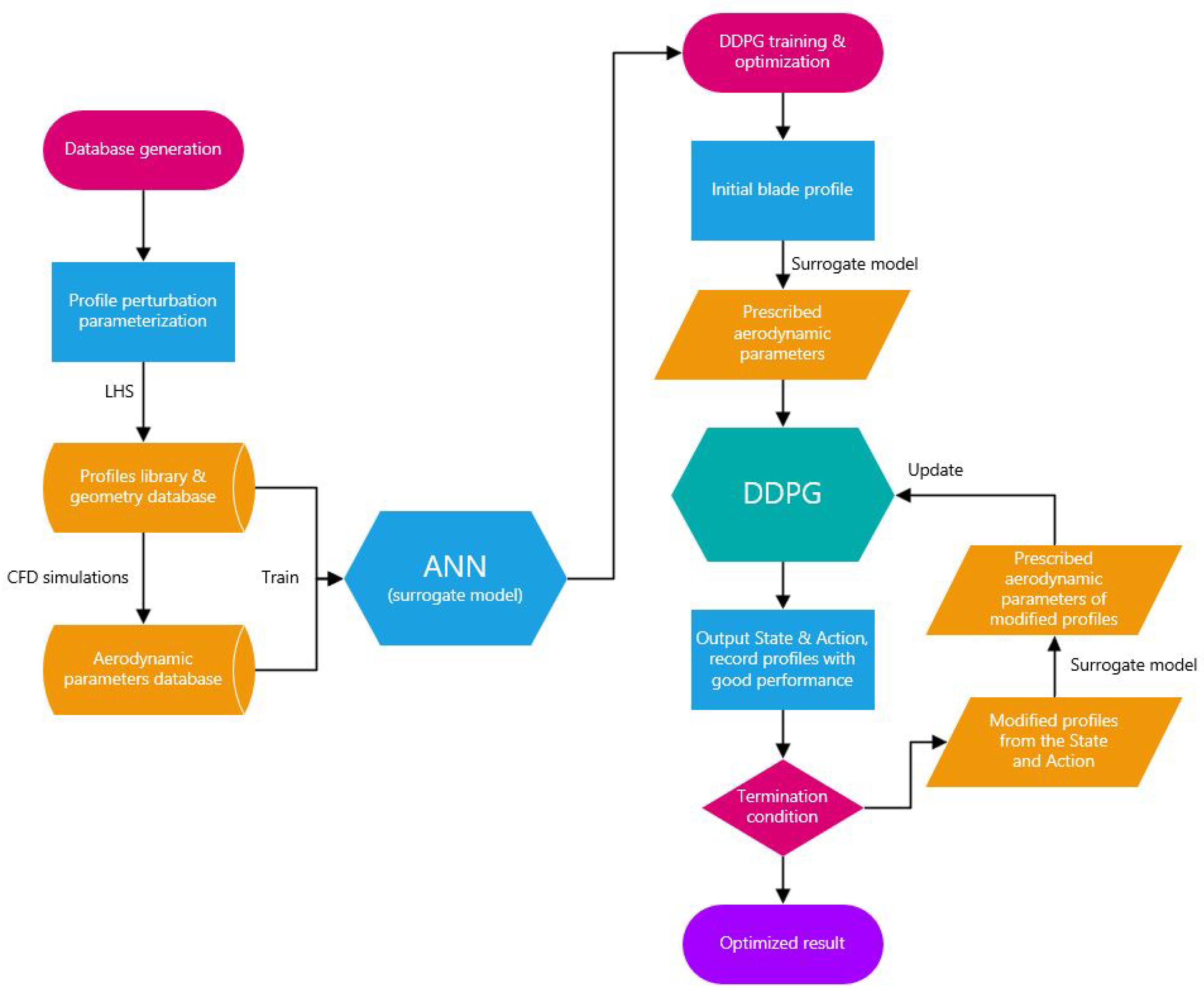
In order to reduce the computation and shorten the optimization period, an ANN (artificial neural network)-based surrogate model is used in this paper to approximate high-fidelity CFD simulations [34]. The model is trained with profile geometric parameters and aerodynamic parameters by numerical calculation. The surrogate model is utilized to feed back the aerodynamic information to the DDPG network as the environment in the optimization. To achieve the multiple objectives interconnection, as well as an appropriate objective function, analysis on the objective space, composed of optimization aerodynamic parameters, is done with Principal Component Analysis (PCA) [35]. The flowchart of the optimization is illustrated in Figure 1.
This paper is organized as follows: In Section 2, the parameterization of the blade profile is introduced. In Section 3, the cascade flow field calculation is validated. Section 4 introduces the surrogate model based on ANN. Section 5 introduces the DDPG algorithm, and the optimization application is presented. Section 6 shows the optimization results with some discussions, and the paper is concluded in Section 7.
2. Parameterization of the Blade Profile
The size of the database for training networks grows fast with the increased number of the input and output variables of the networks. For computation reduction, the number of parameters is required to be as few as possible. One approach is to parameterize the perturbation instead of complete blade profile. It is necessary to have an adequate number of variables to ensure geometric accuracy if parameterization is directly applied to complete description of the blade profile. However, the required number is less if the parameterization is applied on the perturbation of the blade profile.
The parameterization is used to obtain a library of modified profiles with related parameters. The parameterization of blade profiles in this paper is achieved by using the Hicks-Henne bump functions to perturb the original airfoil with assigned coefficients. For situations without fitting the leading edge and trailing edge, the shape functions are defined as:
where represents the normalized position of the bump, and w controls the width of the bump (w equals 3 in this paper). The deformed profile curve can thus be described by:
where presents the magnitude of bumps.
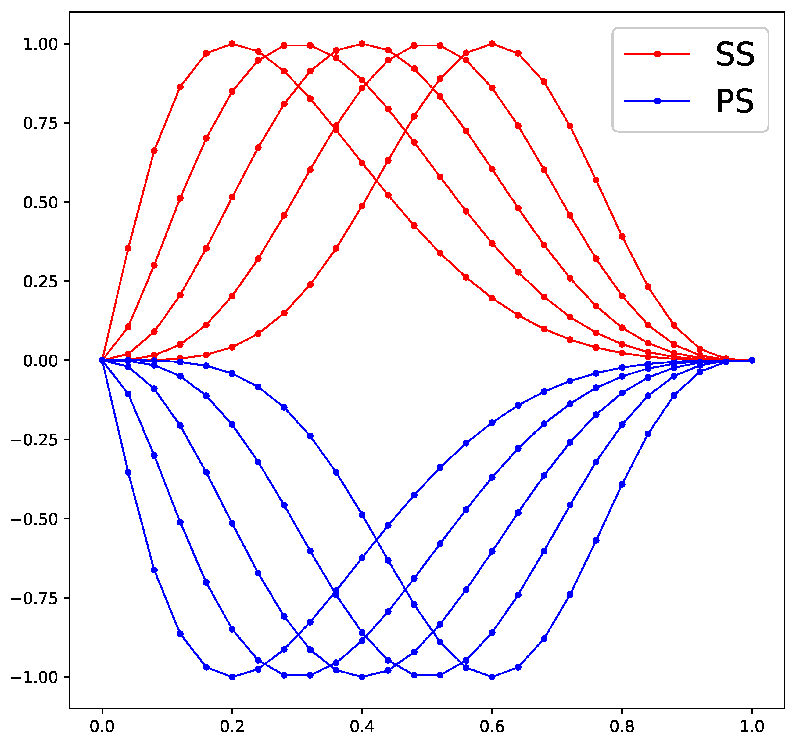
According to previous numerical simulation of the internal flow field of the initial cascade done by the authors, the front middle of the blade suction surface is where the transition and a strong passage shock wave takes place. In order to control the transition position and the passage shock, for both suction surface and pressure surface, five bump functions are used to perturb the profile, and the equals in Equation (1). The shape functions of profile perturbation are shown in Figure 2.
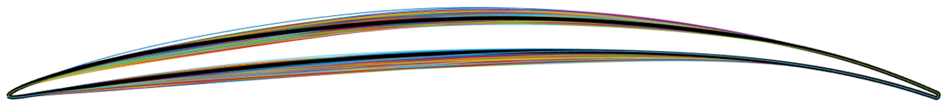
The geometric variable consists of ten coefficients of bump functions . With Latin Hypercube Sampling (LHS), the geometric parameters database is generated, thereby generating the blade profiles library. Ranges of variation of each coefficient are given in Table 1, where and represent expectation and standard deviation of the normal distribution of bump coefficient . The distribution of the profiles is shown in Figure 3.
3. Numerical Method
3.1. Governing Equations, Turbulence, and Transition Model
The governing equations of general Reynolds-averaged Navier–-Stokes (RANS) equations are as follows:
where is the volume, and is the surface of the control volume. The conservative variables , the inviscid flux , and the viscid flux in the time-averaged form can be written as:
Based on Boussinesq’s assumption, the Reynolds stress can be calculated with turbulent eddy viscosity , which is obtained by solving turbulence models.
For turbulence calculation, Spalart-Allmaras turbulence model (SA) coupled with Abu-Ghannam and Shaw transition model (AGS) is used in this paper. SA turbulence model is a one-equation turbulence model proposed and developed by Spalart and Allmaras in 1992 [36]. SA model is often used in the calculation of the internal flow field of turbomachinery ([37,38,39,40], [etc.]) because of its robustness and its ability to treat complex flows [41,42].
The principle of SA model is aimed at solving an additional transport equation for kinematic eddy viscosity. In a non-conservative manner, the equation contains an advective, a diffusive, and a source term. The transport equation is as follows:
The turbulent viscosity is given by
and
where is the turbulent working variable, is the molecular viscosity, d is the distance to the closest wall, and S denotes the magnitude of vorticity. The constants arising in the model are referred to Reference [42].
Abu-Ghannam and Shaw [43] investigated the experimental data of transition on a flat plate with pressure gradients and proposed the model to compute the location of transition from the flow solution by using empirical relations related to external parameters. The AGS model dictates that transition starts at a momentum thickness Reynolds number:
The dimensionless pressure gradient is defined as:
where is the velocity at the edge of boundary layer, S is the streamwise distance from the leading edge, and denotes the momentum thickness in the laminar region.
For the SA model, the free stream turbulence level is computed based on the upstream eddy viscosity and assuming a turbulent length scale of about of the reference length scale:
The function depends on the pressure gradient:
3.2. Cascade Performance Calculation
The three-dimensional compressible Navier–Stokes equation is solved by using a finite-volume based RANS solver NUMECA FineTurbo. Multigrid technique is used during the solving process in order to accelerate the convergence.
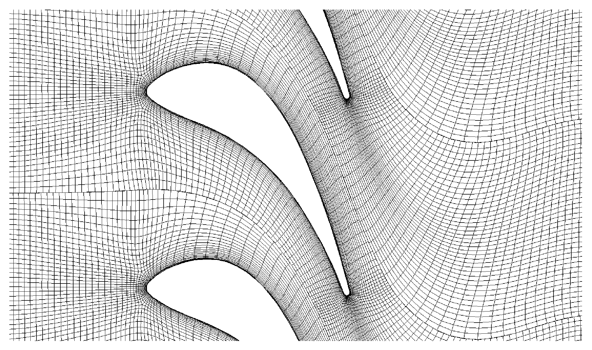
To test the accuracy of the transition position prediction, the VKI turbine blade is chosen as the validation case. The VKI turbine blade, as is shown in Figure 4, has been investigated a lot, both numerically and experimentally, and the experimental data on its transition position can be referred to in Ubaldi [51]. The blade-to-blade grid used to validate the calculation is shown in Figure 5.
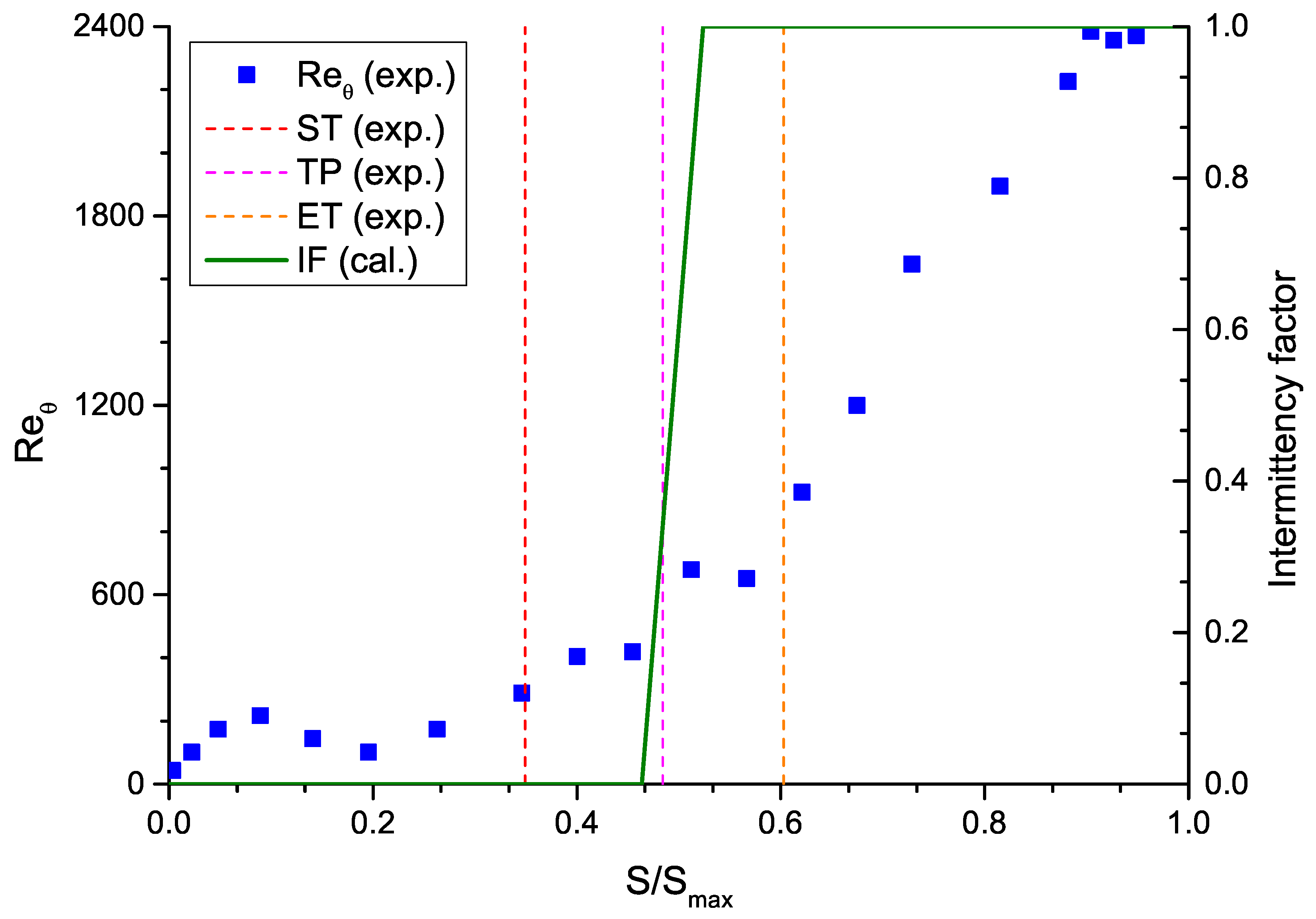
Figure 6 shows the experimental and the calculated data of the transition position of VKI turbine. The experiment was carried out by Ubaldi [51]. Details about experimental measurement can be referred to in Appendix A.1. With Laser Doppler Velocimetry (LDV), the boundary layer integral parameters distribution is measured, and the start of transition (ST), transition position (TP), and end of transition (ET), marked in Figure 6, were concluded by Ubaldi, according to the boundary layer integral parameter distributions from the experiment [51]. The intermittency factor is used to trigger the transition locally, which is computed on each point of the blade surface and at each iteration via the solver. The intermittency factor is 0 before transition and 1 after the transition onset. According to the calculated intermittency factor distribution in Figure 6, the computational transition position fits well with the experimental transition position (magenta dashed line in Figure 6), which validates the accuracy of the calculation of transition position.
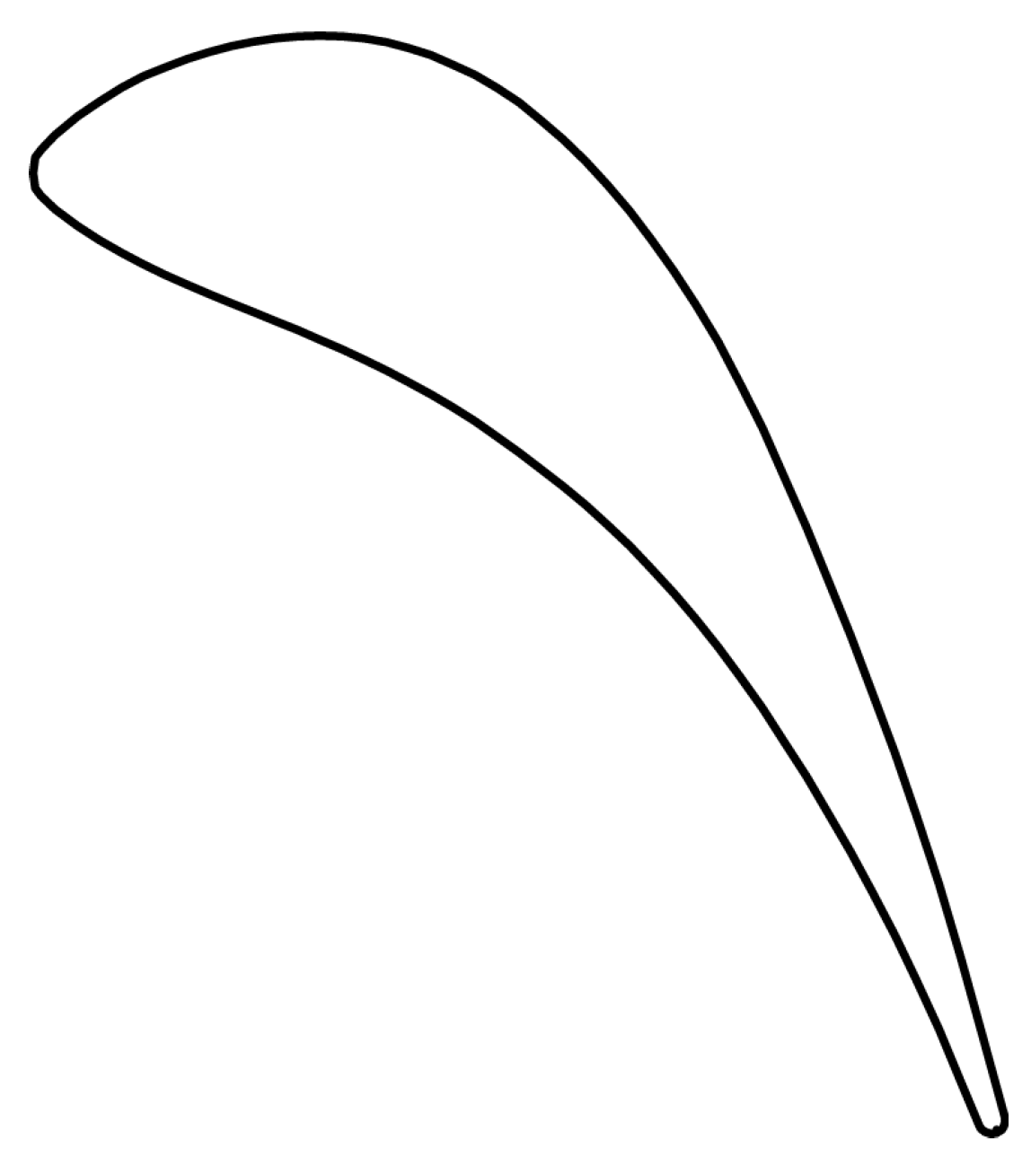
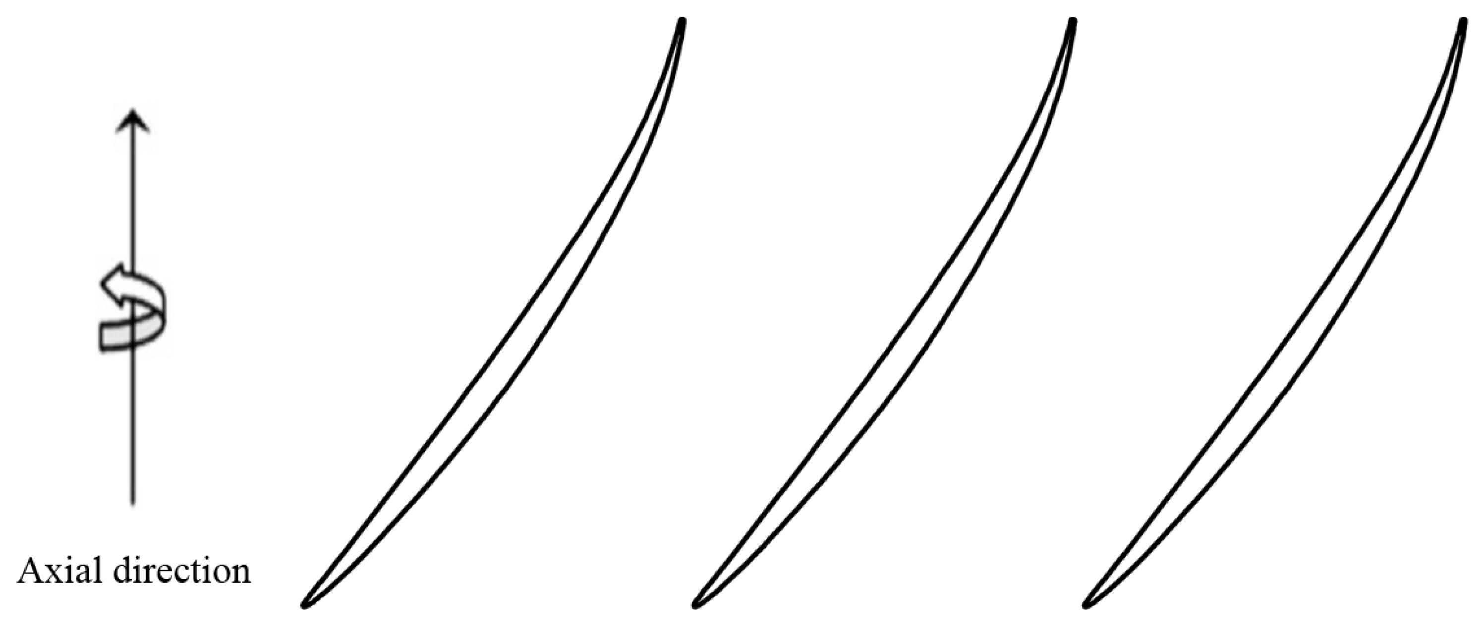
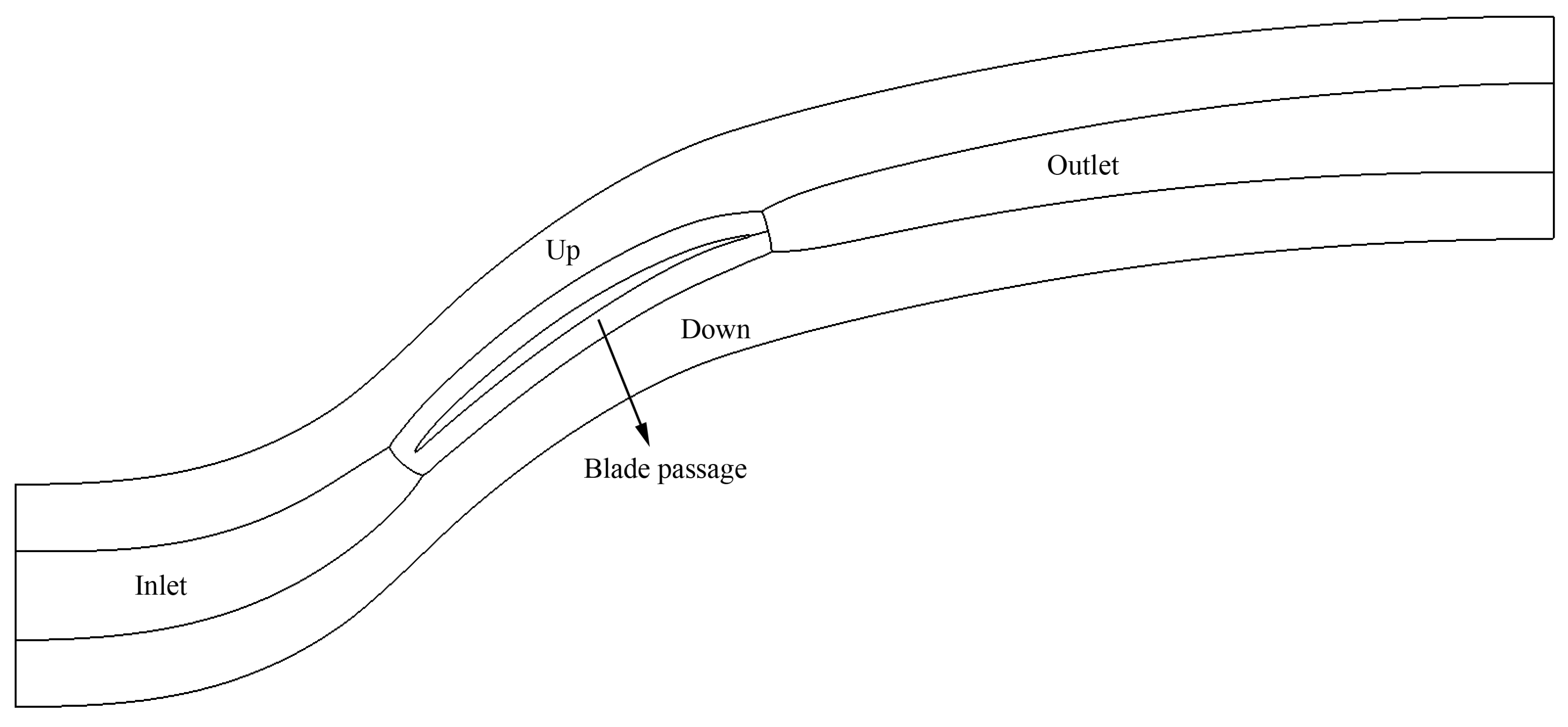
The geometry of the initial cascade blade profile to be optimized in this paper is shown in Figure 7, with the basic parameters listed in Table 2. The blade-to-blade grid is generated as a structured grid, with the topology shown in Figure 8. The length of the inlet domain is as long as the chord line, and the outlet domain is twice as long as the chord line.
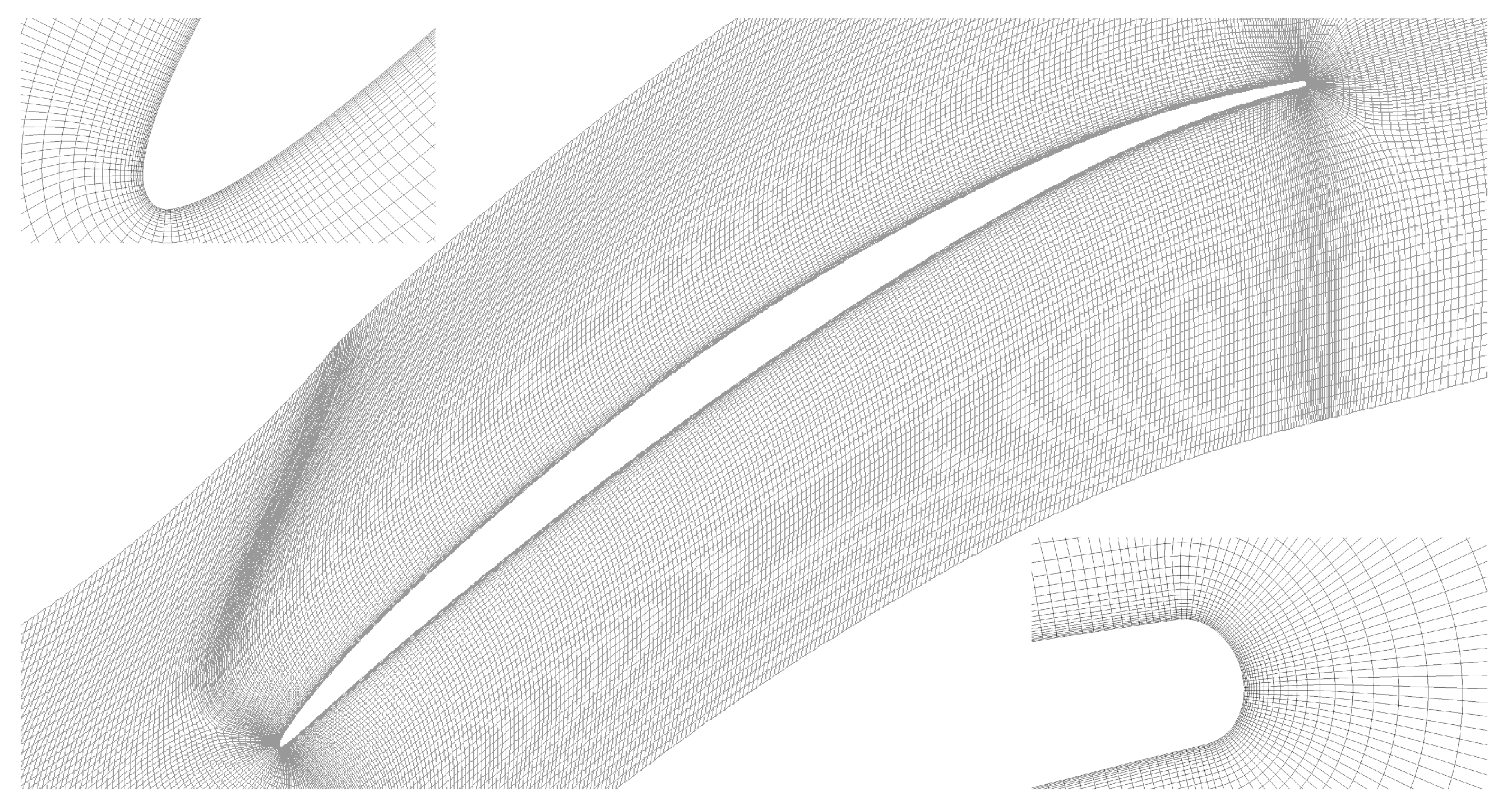
A three-dimensional grid is used as the cascade grid, with five points across the span of the cascade, generated via NUMECA AutoGrid. The boundary condition at the hub and shroud is set to the mirror boundary condition, to eliminate the three dimensional effect. The grid points distribution is listed in Table 3. The total number of grid points is . The height of the cells at the walls is set to m to ensure that is below 10. The 2D cross-sectional view of the computational grid is shown in Figure 9.
At the inlet boundary, the total pressure, the total temperature and the flow angle are specified. The total pressure of 119,600 Pa and the total temperature of 293 K are given at the inlet boundary. At the outlet boundary, the static pressure at standard sea level was specified. On the solid wall boundary, the no-slip and adiabatic conditions were used. In these conditions, the cascade flow is examined with an inlet Mach number of at the operating point (). From the simulation, the relative laminar region at the operating point is at the suction surface (SS) and at the pressure surface (PS).
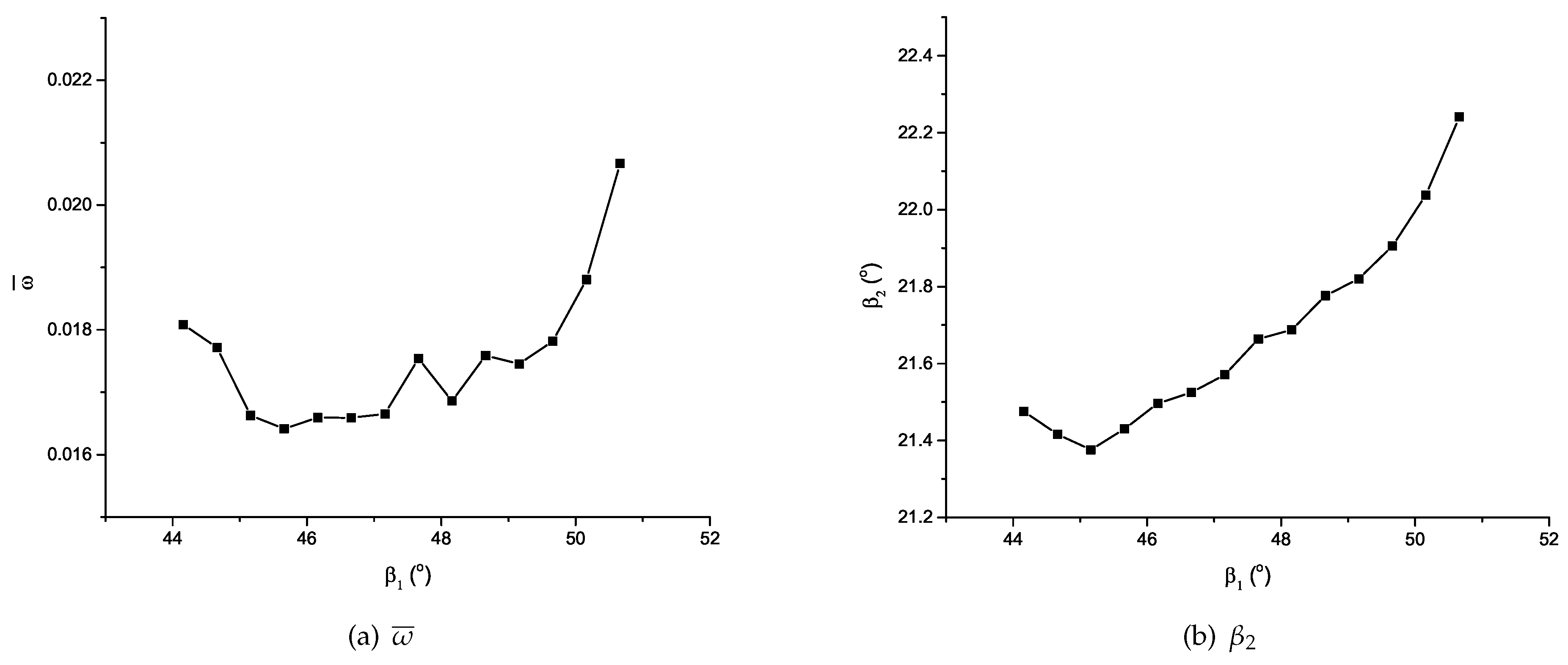
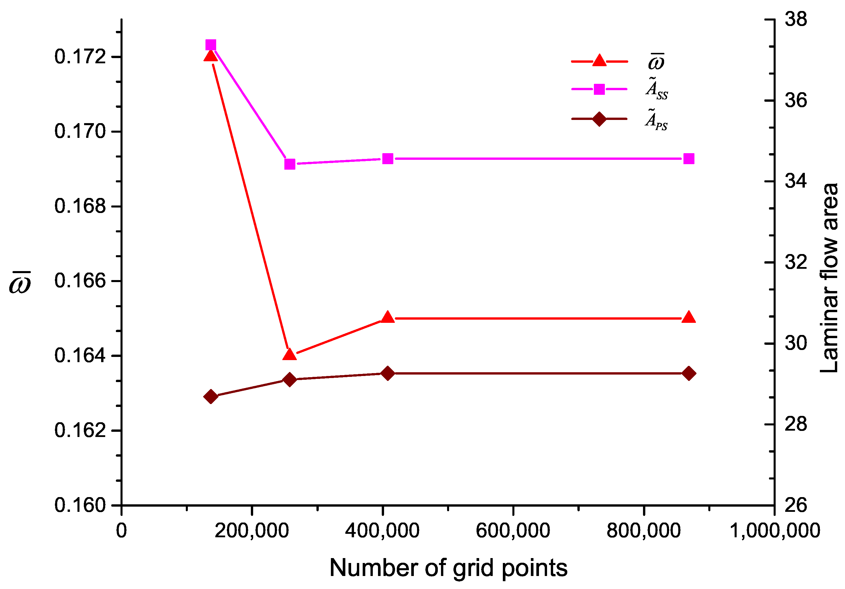
In this paper, total pressure loss coefficient is defined as: , where and are the total pressure of the inflow and outflow. is the static pressure of the inflow. From multiple computations with the inlet flow of the same Mach number and different , the aerodynamic performance curve can be obtained, as in Figure 10. The operating point is at the inlet flow angel of , and the operating range is from to for . The result of grid independence test is shown in Figure 11.
4. Surrogate Model Based on ANN
The optimization, especially with multiple objectives, are computationally intensive and time-costly. Using a surrogate model to approximate and replace high-fidelity CFD simulations is necessary for the complicated optimization of aerodynamic shapes. Surrogate models can provide aerodynamic information rapidly, which reduces the computation during optimization and shortens optimization period [52,53]. It is attractive for complex multi-objective optimizations for turbomachineries and is used in blade shape optimizations [54,55]. ANN has excellent nonlinear mapping and learning ability, which makes it advantageous in approximating the strong nonlinear relationship bewteen the geometric shape and multiple simulated aerodynamic parameters [34,56]. Using ANN as the surrogate model, with prediction instead of computation, eliminates the need for CFD simulations during optimization, which improves optimization efficiency and automation [56].
In this paper, a surrogate model based on ANN is used to predict the total pressure loss coefficients, outlet flow angles, and laminar flow areas of the deformed blade profiles. One separate neural network is used for prediction of each aerodynamic parameter. During the training process of the DDPG, the surrogate model acts as the role of environment, giving the predicted aerodynamic parameters and calculating the reward of the given action and state.
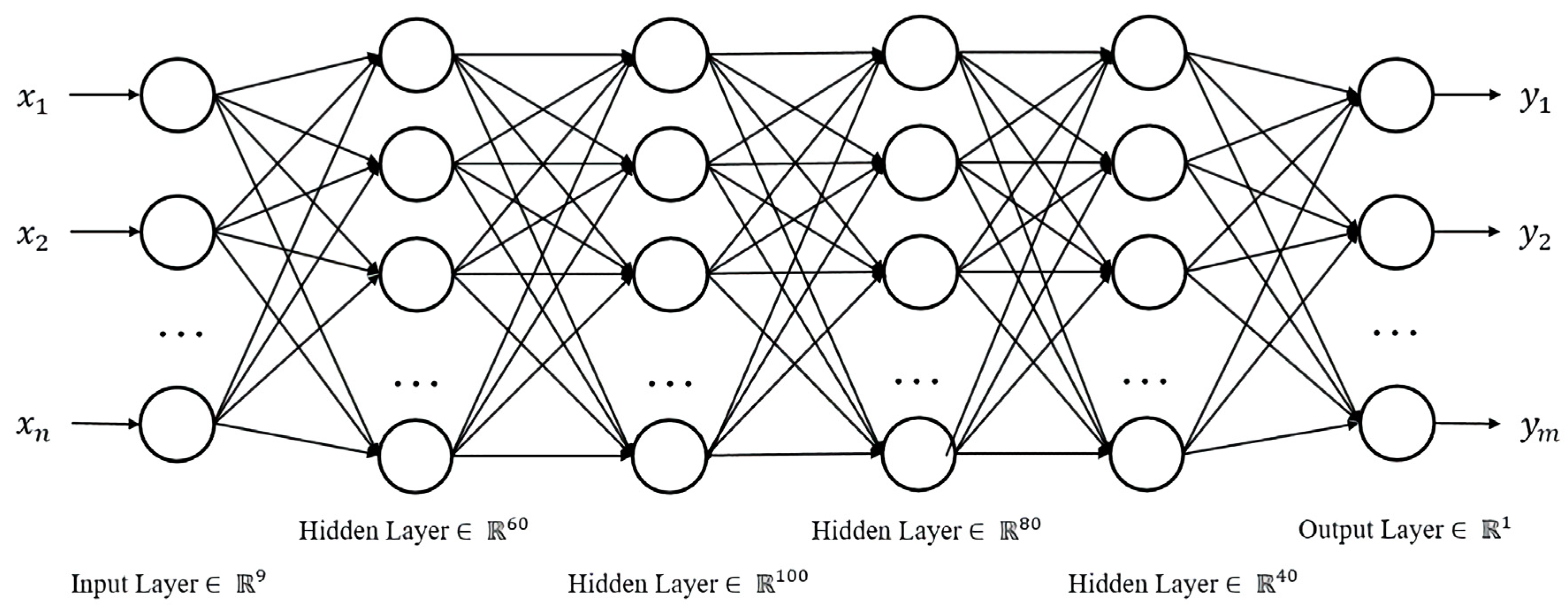
The structure of the neural network used in this paper is shown in Figure 12. The input variables are the geometrical parameters, and the output variable is the aerodynamic parameter. The network has a six-layer structure with four hidden layers. The numbers of nodes of the four hidden layers are , respectively. The selection of the ANN structure, including the number of hidden layers and the number of nodes in each hidden layer, is experience-based [57]. In this paper, referring to Reference [34], the structure is defined by adjusting and trying many times. The activation function of each layer is ReLU (Rectified Linear Unit) function , in which the expression can be written as: . The data is divided into a training set and test set . The optimizer of the network is Adam [58]. The learning rate is set as to make sure the network converges fast.
Since the transition location and the total pressure loss vary consistently in a small range near the design point when the modification is reasonable and small, while the outlet flow angles vary less consistently over the operating range, the total pressure loss coefficient and the laminar flow areas at the operating point and multiple on-design and off-design outlet flow angles are considered in the optimization. One network with the above structure and hyperparameters is built and trained for each output variable in aerodynamic parameters (, , , of in ()). The trained networks can represent the correspondence between geometric data and aerodynamic data. The aerodynamic parameters of one specific deformed rotor can be predicted easily by feeding the geometric parameters to the trained networks.
5. DDPG-Based Optimization for Blade Profile
5.1. Deep Deterministic Policy Gradient (DDPG)
In this paper, DDPG [32] is used as the intelligent designer to find the optimial policy for the multi-objective design of cascade blade. DDPG is one reinforcement learning algorithm which can choose the appropriate action according to specific state. Different from the value-based learning methods, e.g., deep Q-learning (DQN), which is restricted to discrete and low-dimensional state and action space, DDPG can handle the high-dimensional complicated action problems with the continuity of state and action space.
DDPG is developed from DPG, by using deterministic policy instead of random policy [31]. Since the policy is deterministic, the output action is determined according to the input state and does not need to be sampled from a probability distribution. Therefore, the calculation of internal expectation for policies is avoided, and external expectation only needs to be calculated according to the environment. The computational resources are saved, and the variance becomes small, improving the convergence.
DDPG is a policy gradient method with an actor-critic structure [59]. The actor network approximates to the deterministic policy function , which learns a policy that yields the highest possible reward so that a definite action from the current state can be given. The critic network approximates the action-state value function to criticize the given action, according to the action in state and following policy . With the network parameter , the critic network can be written as . The actor network can be written as with parameter . With the value function, the actor network can be updated by the gradient of the policy , according to the deterministic policy gradient theorem:
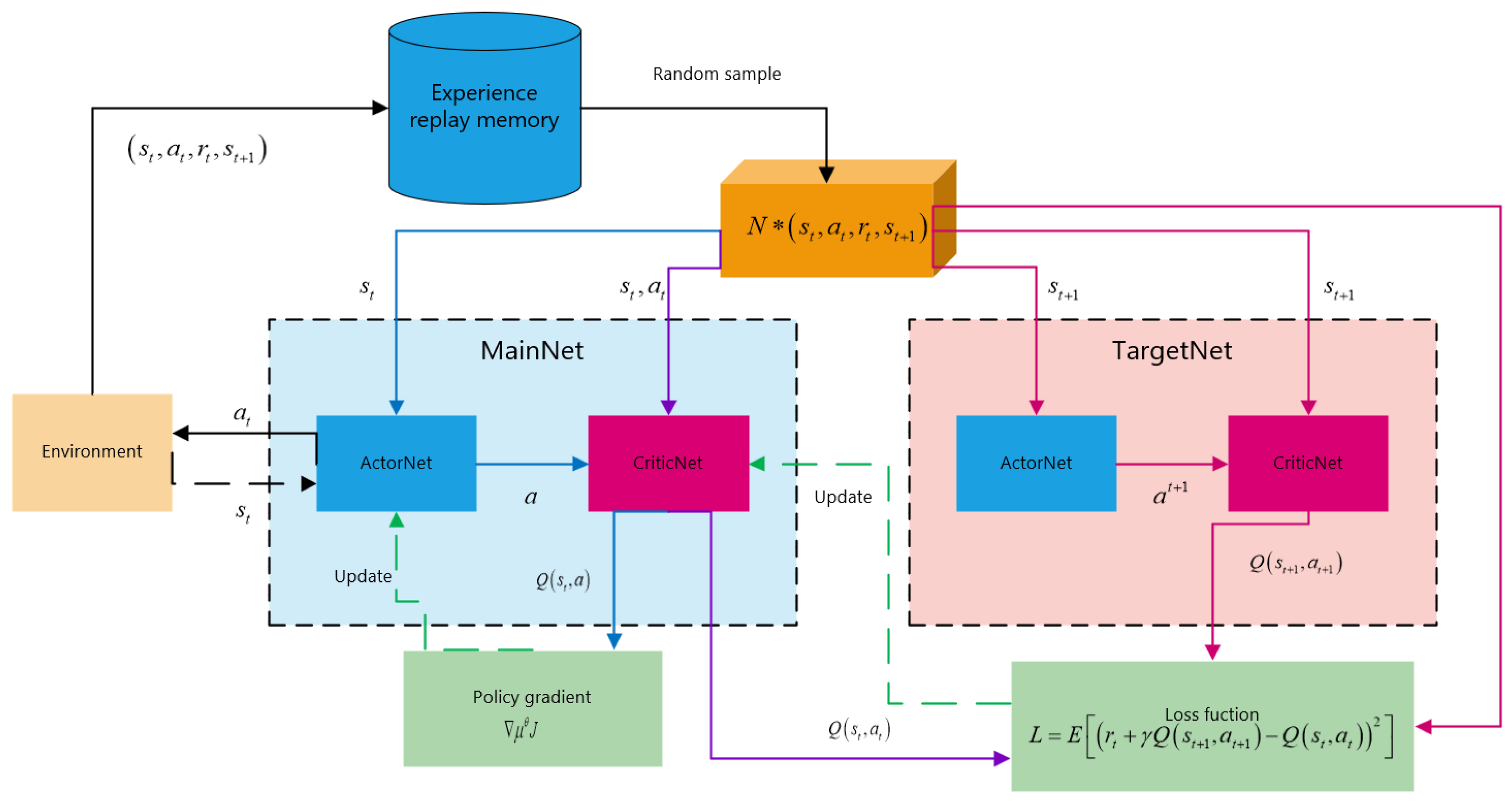
Drawing on the idea of DQN, DDPG has two frameworks of actor-critic structure: main framework and target framework. Each framework contains one actor network and one critic network. The main actor network gives the action . The main critic network outputs the value function and updates the actor network. The action is performed in the environment, to achieve the next moment state and the calculated reward . The target framework stores the fixed target networks. The target actor network gives according to the state and the policy . The target critic network outputs the value . When the target networks are updated, soft update is used: ,, where is the soft-update parameter. Therefore, the target network parameters can be updated slowly, with improved learning stability. The main critic network is updated to minimize the loss function:
DDPG uses an experience replay memory to store transitions from interacting with the environment. The experience transitions are stored in the memory and then fed to update the networks in batches with a random sample strategy. Random sampling can eliminate the correlation between transitions, improving the stability of network training. The structure of DDPG is shown in Figure 13.
Based on DPG, DDPG uses deep neural networks. A multilayer feed-forward network with enough neurons in hidden layers can approximate any continuous function with arbitrary accuracy [60]. With the deeper network structure, the actor and the critic network can approximate the policy and the value function more accurately. The deeper network structure also increases the dimension of action that can be handled. But, for problems with complex action space, increasing the number of hidden layers and the number of nodes of each layer may increases the training time of the network, and even lead to the tendency of over-fitting.
5.2. Application of DDPG and Optimization
DDPG is used in this paper to approach optimization policies. Since the optimization is to achieve the blade profile with the optimal aerodynamic parameters by modifying the geometry, it is suitable to take the geometric parameters space as the state of DDPG network, and to choose the variations of geometric parameters as the action.
The hyperparameters of the DDPG network are as follows: The target smoothing coefficient is 0.005. The discounted factor is 0.99. The batch size equals 64, and the replay buffer size equals 50,000. The learning rate is selected as 0.01, to make sure the network can converge faster. The other hyperparameters are selected by referring to Reference [61,62] with little adjustment, which is common and widely-used in the applications of DDPG. The hyperparameters are selected in order to ensure the actor and critic networks can converge and the DDPG network can achieve high rewards.
For multi-objective optimization, the analysis of objective space can help us better understand the relationship between optimization variables, which is directly associated with a more problem-oriented formulation of optimization objective. The aerodynamic parameter database generated to train the network can provide a large number of samples for objective space analysis. Principal Component Analysis (PCA) [63] is an effective tool to extract the main modes from objective space considered to be the essential information that may help establish a more reasonable optimization objective.
For blade profiles in the profile library sampled corresponding to given n, the aerodynamic parameters of n profiles achieved through CFD simulation constitute a database represented in Equation (14), where the eight columns are the total pressure loss, relative laminar flow areas, outlet flow angles of different inlet flow angles, respectively. To compare the parameters according to the principal component, the aerodynamic parameters in are normalized. To obtain the relative distribution matrix , Each column of the data matrix is subtracted from the mean value of the column. According to Equation (15), the data from objective space systematically forms the covariance matrix . The eigendecomposition is shown in Equation (16), where represents diagonal matrix of eigenvalues and represents agglomeration of eigenvectors.
Through the analysis of eigenvectors, the relationship between the parameters in the multi-objective optimization of the cascade blade can be known and help to determine the reasonable reward function of reinforcement learning method and appropriate objective function of optimization. The first and second principal component of the aerodynamic data are listed in Table 4. The first principal component represents the internal relation of outlet flow angle variations. The second principal component contains information: the decrease of total pressure loss coefficient has a strong dependence on the increase of laminar flow area. It may be inferred that the increase of laminar flow area is beneficial to the reduction of total pressure loss, and the influence of the laminar flow area of the suction surface is much greater than that of the pressure surface.
The environment of the DDPG network in this paper is the ANN-based surrogate model. With the given state and action (the profile geometry and geometric change), the next step state (updated geometry) can be obtained. The aerodynamic parameters according to the state and action can be predicted with the surrogate model, to calculate the reward function . The reward function represents our actual evaluation of an action. It is used to adjust the critic network to output value function closer to reality. Since a blade profile is expected with lower total pressure loss coefficient, larger laminar flow area, and as small as possible change in outlet flow angle, the reward function can be expressed as:
where , and and are boundaries to constrain of different . , , and represent the initial profile’s , , and . According to the PCA, the weights in Equation (17) are: .
The target of the optimization is to achieve a blade profile with reduced total pressure loss and improved laminar flow area. During the training process of the DDPG network, huge numbers of states (profiles) interact with the environment, many of which have good performance. Each time the reward value of one state is calculated, the aerodynamic parameters of the blade profile of the state are predicted by the surrogate models. The state (the geometric parameters) of the blade profile with the smaller objective function is stored in the training process of the DDPG network to optimize the blade profile. Compared with the initial blade profile, the optimized blade profile should have as small total pressure loss coefficient as possible, enough large laminar flow area, and enough small change in outlet flow angle, so the objective function of the optimization can be expressed as:
with a constraint on . The weights are: .
With the optimization policy from DDPG, the optimizer can approach the good-performance profile (high reward state) with not many iterations of geometric modification (action).
6. Results and Discussion
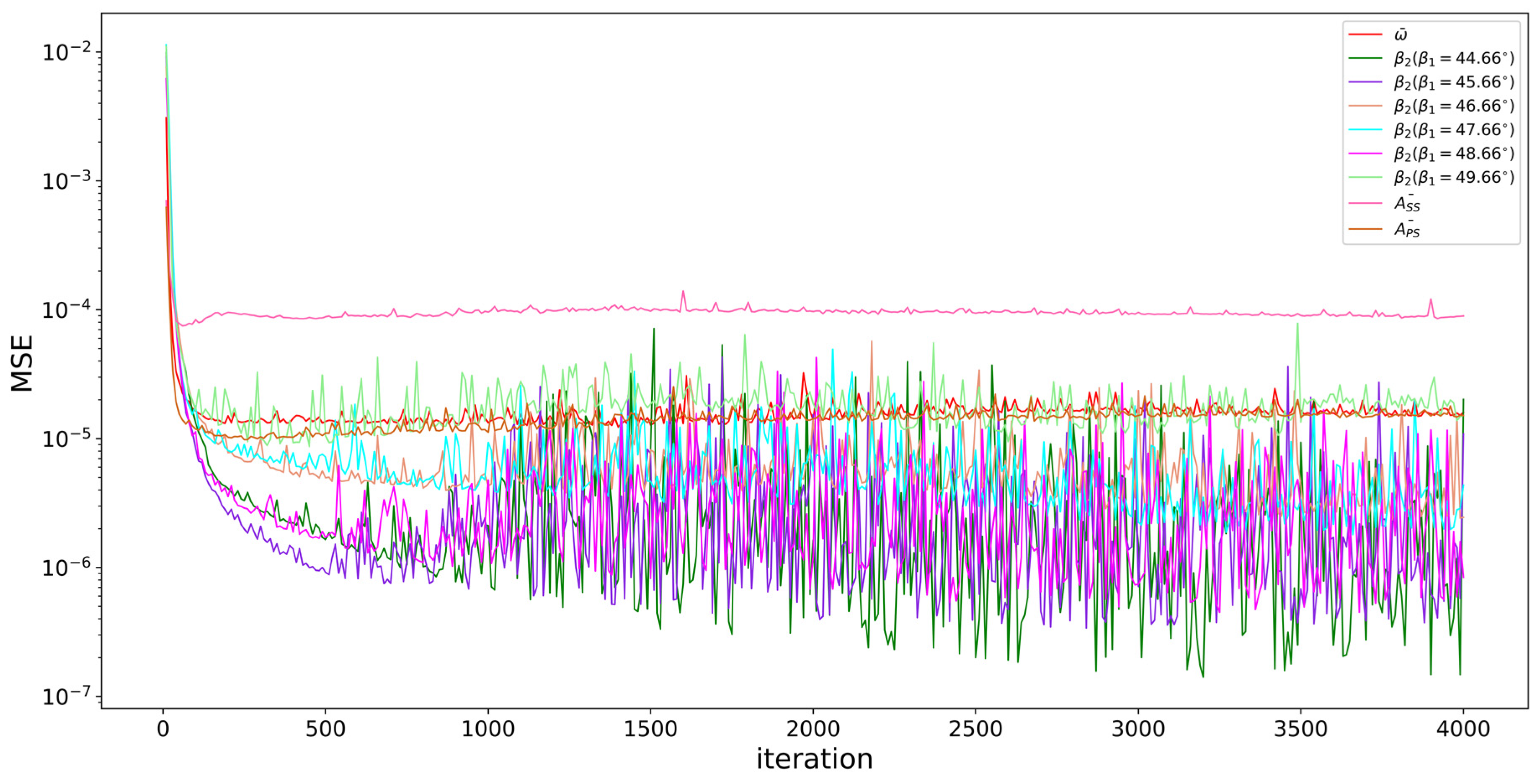
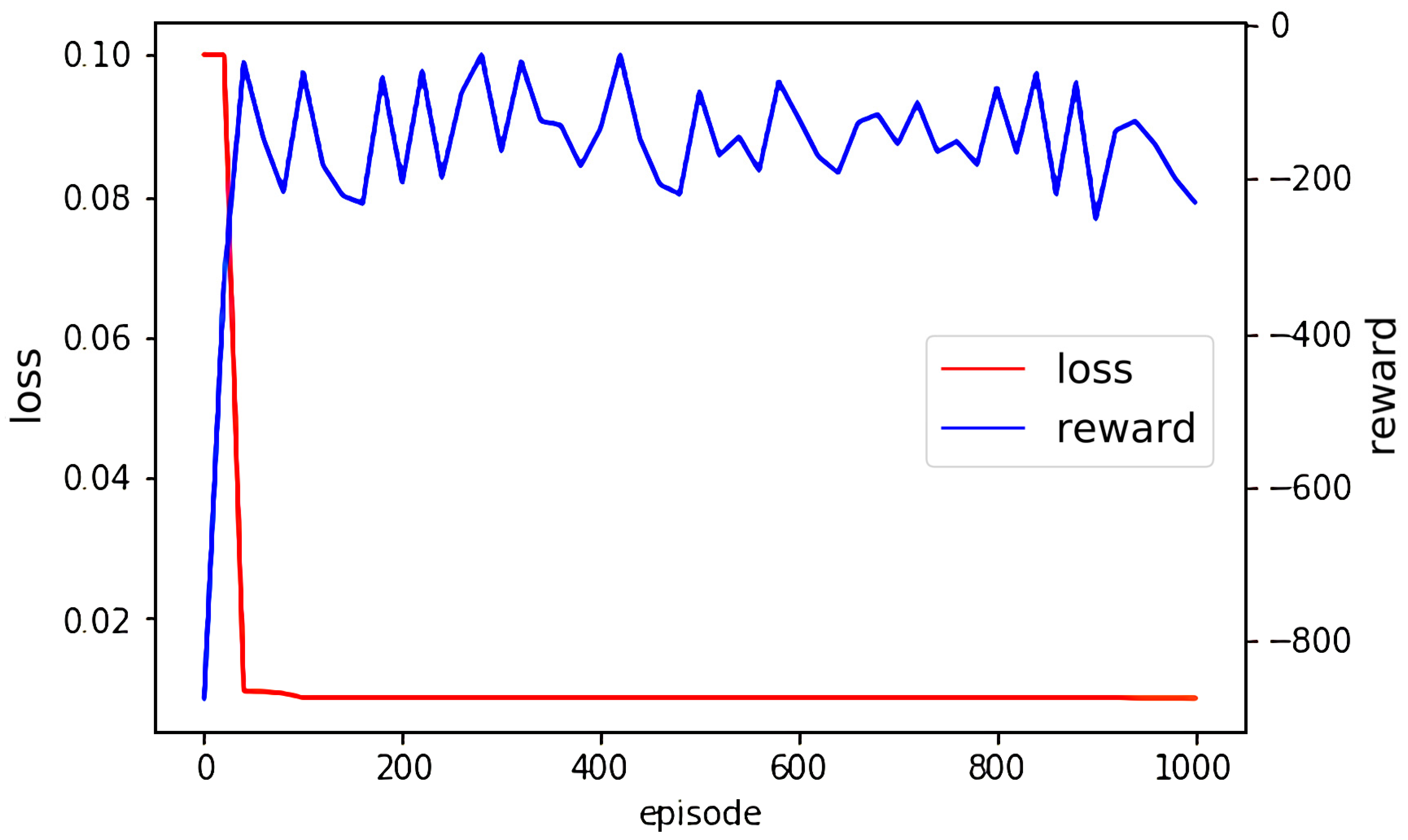
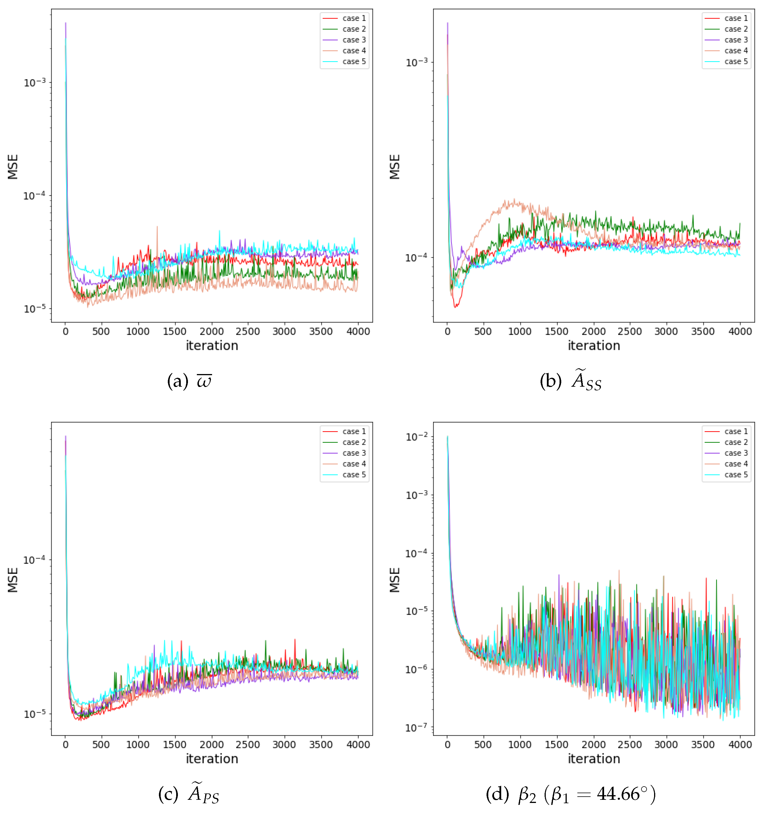
The convergence curves of the neural networks are shown in Figure 14. The aerodynamic parameters, except , have a good convergence result with MSEs (mean square errors) by less than . varies much for profiles in the profile library; thus, it does not converge as well as other parameters, but it is still within small MSE of . The small convergence errors show that the ANNs have good performance of prediction on the test sets. The independence study of division of train-set and test-set is shown in Appendix A.2. Figure 15 shows the reward curve of the DDPG algorithm and the objective function curve of the optimization. The DDPG network can be trained well and obtain a high reward in 100 episodes. With the trained DDPG network, the optimizer can find and record a profile with very good performance in no more than 200 episodes, which, as it turns out, means that this optimization method based on DDPG can rapidly achieve a fairly good result. The better-performance profile updates slow and varies slightly after 200 episodes, as well as the objective function.
With the ANN-based surrogate model and the DDPG based optimization, a new rotor blade profile with lower total pressure loss coefficient and larger laminar flow area is achieved. By CFD validation, the performance characteristics and the flow field characteristics of the cascade with the optimized blade profile can be known and compared with the original cascade.
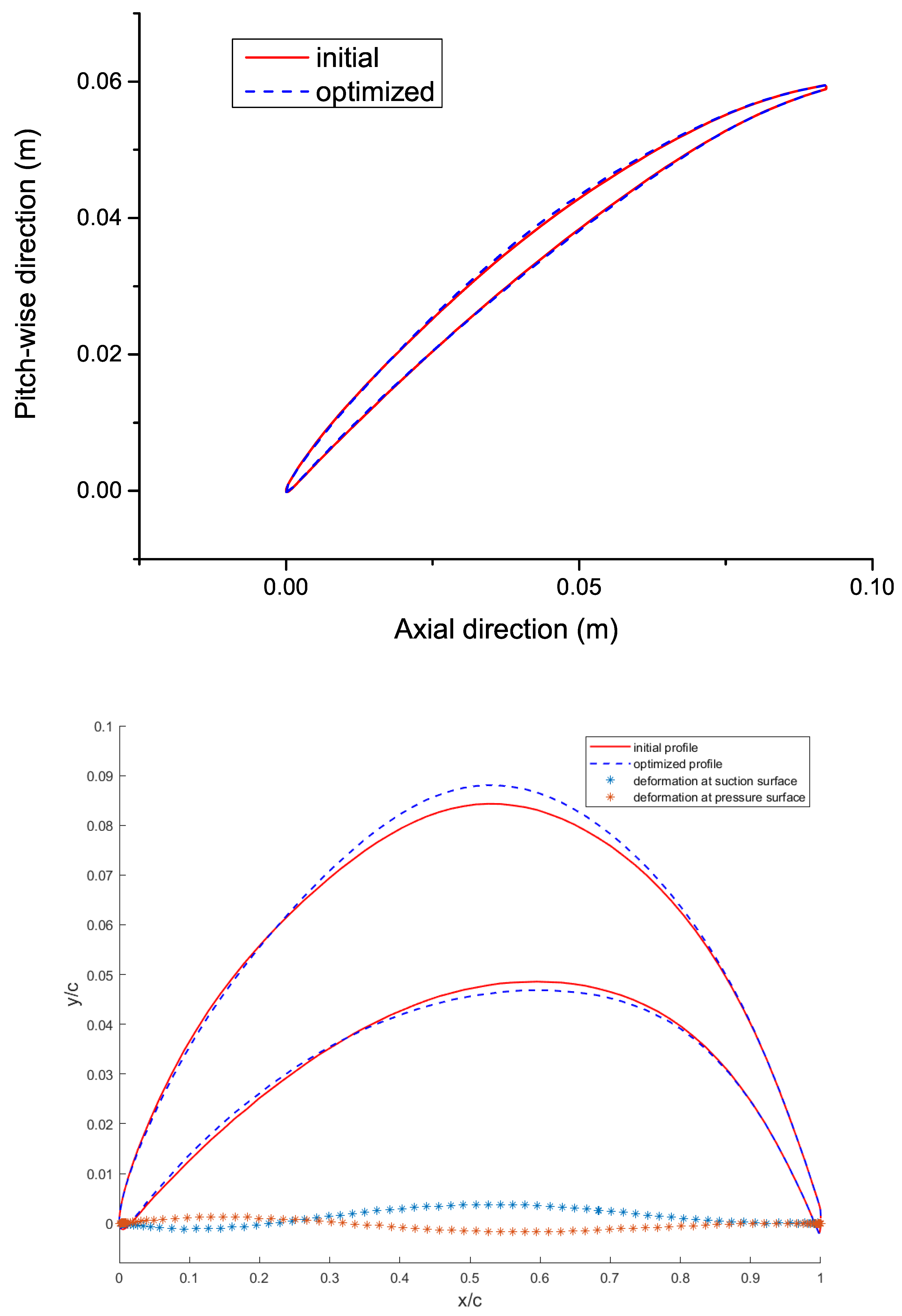
Figure 16 shows the original and the optimized rotor blade profiles. Compared to the initial profile, the optimized profile has following characteristics: (1) The thickness of the front of the profile is slightly reduced; (2) the thickness of the middle part of the profile is increased, where the thickness at the pressure surface is increased slightly resulting in a flatter shape, and the thickness and curvature at the suction surface is obviously increased.
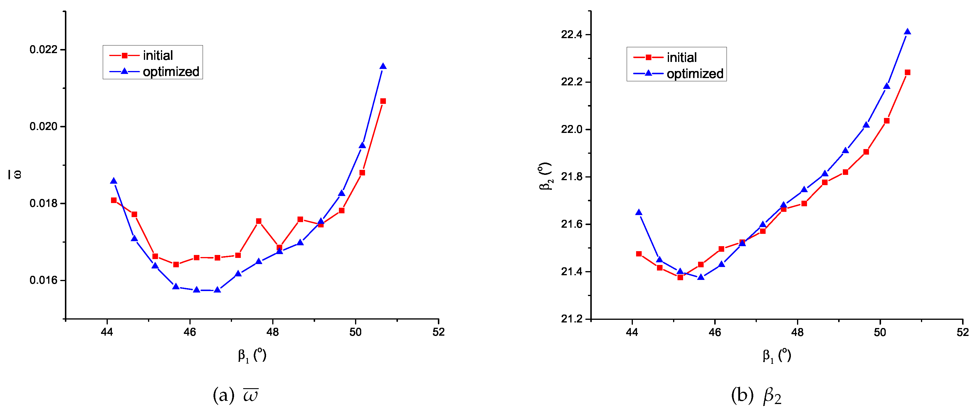
The aerodynamic performance curves of the cascades of the original blade profile and the optimized profile are shown in Figure 17, respectively. In the operating region, with being to , of the cascade with the optimized blade profile decreases considerably, with a relative reduction up to . The variation of is small, and the relative change in the operating region is no more than .
The performance characteristics of the cascades at the operating point are listed in Table 5. of the cascade goes from to , with a relative reduction of . The relative laminar flow area at the suction surface rises from to , with massive increase. The relative laminar flow area at the pressure surface is basically unchanged. It can be concluded from the results that the DDPG-based optimizer successfully optimized the cascade blade profile with relatively being reduced, and higher than the initial profile. The large improvement of is in line with the information from the PCA that contributes more on reducing than (cf. Table 4). CFD simulation and ANN prediction on performance characteristics of the initial and optimized cascades are compared in Table 6. Compared to the CFD results, the ANN prediction has an error of about on the total pressure loss coefficients and an error of about on the laminar flow areas, which proves that the ANN-based model can accurately predict the aerodynamic performance
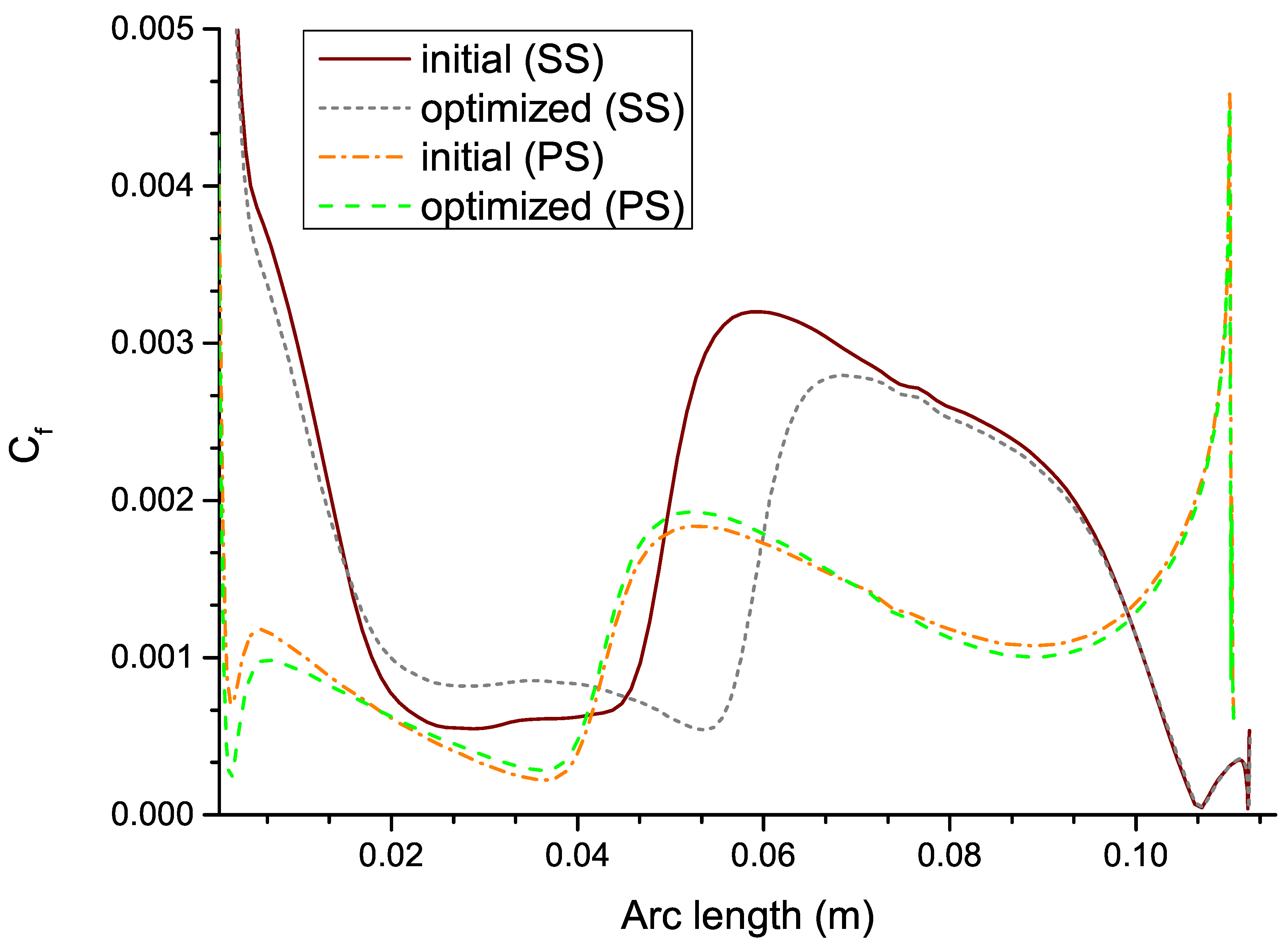
Figure 18 shows distributions on suction and pressure surfaces. Compared with the initial profile, the position of the jump of is moved aft at the suction surface, which indicates an obvious delay of transition. The distributions on pressure surfaces are basically the same, consistent with the laminar flow areas obtained with the intermittency factor distributions, as in Table 5.
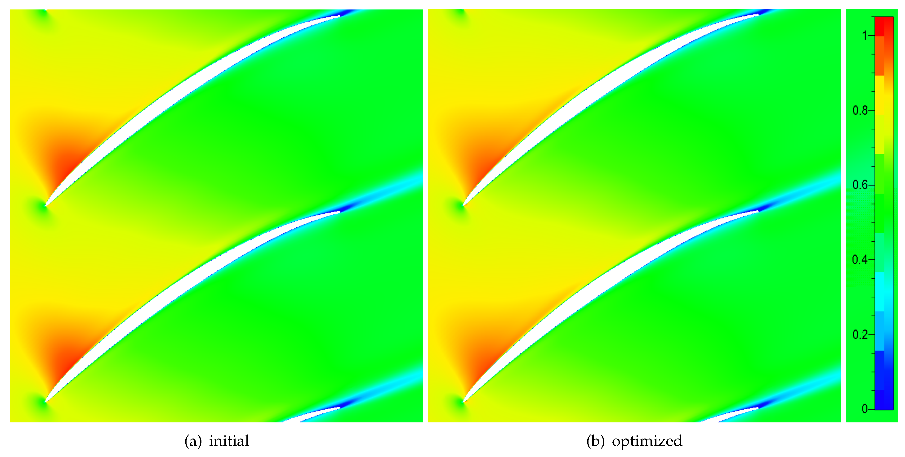
The absolute Mach number contours of the original and the optimized blades are plotted in Figure 19. Compared with the initial profile, the shock wave at the suction surface is weakened and moved aft. This results in a reduction in shock loss, which is also a contribution to the decrease of the total pressure loss.
7. Conclusions
In this paper, a multi-objective optimization method based on reinforcement learning technique is proposed and applied in a hybrid optimization of the compressor cascade blade profile on the total pressure loss and the laminar flow area. Firstly, an ANN-based surrogate model is used as the environment in the DDPG network, feeding back the aerodynamic parameters corresponding to the deformed profiles with surrogate model trained with parameterized profiles and aerodynamic data calculated via CFD solver. Secondly, based on the reinforcement learning technique of DDPG, a multi-objective optimization method is proposed, where the profile geometry is taken as the State of the DDPG network, the modification of geometry is taken as the Action, and the DDPG network acts as an intelligent optimizer learning the design experience from the interaction with the environment. The optimizer can approach the good-performance profiles rapidly according to the learnt design experience.
With the optimization on total pressure loss and laminar flow area, the cascade with modified blade profile has an improved performance and increased laminar flow area. The total pressure loss coefficient of the optimized profile is reduced by , and the relative laminar flow area at the suction surface is higher than the initial profile. The result shows that the DDPG-based method is one successful multi-objective optimization of cascade blade profile, with an improvement on using the accumulated calculation data to extract design experience and making design policies for guiding optimization. The cascade blade profile optimized in this case is the section profile at span of one compressor rotor blade. This optimization method can be applied to profiles at different spans of the rotor. With multiple profiles at various spans considered, this method can be extended to 3D shape optimization method and be applied to 3D rotor blades.
Author Contributions
Conceptualization, S.Q.; methodology, S.Q. and S.W.; software, S.Q. and C.W.; validation S.Q.; formal analysis, S.Q. and L.W.; investigation, S.Q., L.W. and C.W.; resources, Y.Z.; writing–original draft preparation, S.Q.; writing–review and editing, S.W.; visualization, S.Q. and S.W.; supervision, G.S.; project administration, G.S.; funding acquisition, G.S. All authors have read and agreed to the published version of the manuscript.
Funding
This research was funded by AECC Commercial Aircraft Engine in the project of Laminar Flow Design and Turbulent Drag Reduction of Compressor Blade Profile and Experimental Verification.
Institutional Review Board Statement
Not applicable.
Informed Consent Statement
Not applicable.
Data Availability Statement
The data presented in this study are available on request from the corresponding author. The data are not publicly available due to privacy.
Conflicts of Interest
The authors declare no conflict of interest.
Abbreviations
The following abbreviations are used in this manuscript:
| DDPG | Deep Deterministic Policy Gradient |
| RL | Reinforcement Learning |
| DRL | Deep Reinforcement Learning |
| DQN | Deep Q-learning |
| CFD | Computational Fluid Dynamics |
| PCA | Principal Component Analysis |
| ANN | Artificial Neural Network |
| LHS | Latin Hypercube Sampling |
| MSE | mean square error |
| SS | suction surface |
| PS | pressure surface |
| IF | intermittency factor |
| coefficients of bump functions | |
| expectation of | |
| standard deviation of | |
| S | surface distance measured from leading edge |
| surface length from leading to trailing edge | |
| inlet flow angle of cascade | |
| outlet flow angle of cascade | |
| total pressure loss coefficient | |
| relative laminar flow area at suction surface | |
| relative laminar flow area at pressure surface | |
| skin friction coefficient | |
| aerodynamic parameter * of the initial blade profile | |
| aerodynamic parameter * of the optimized blade profile |
Appendix A
Appendix A.1. Details of Experimental Measurement of Ubaldi
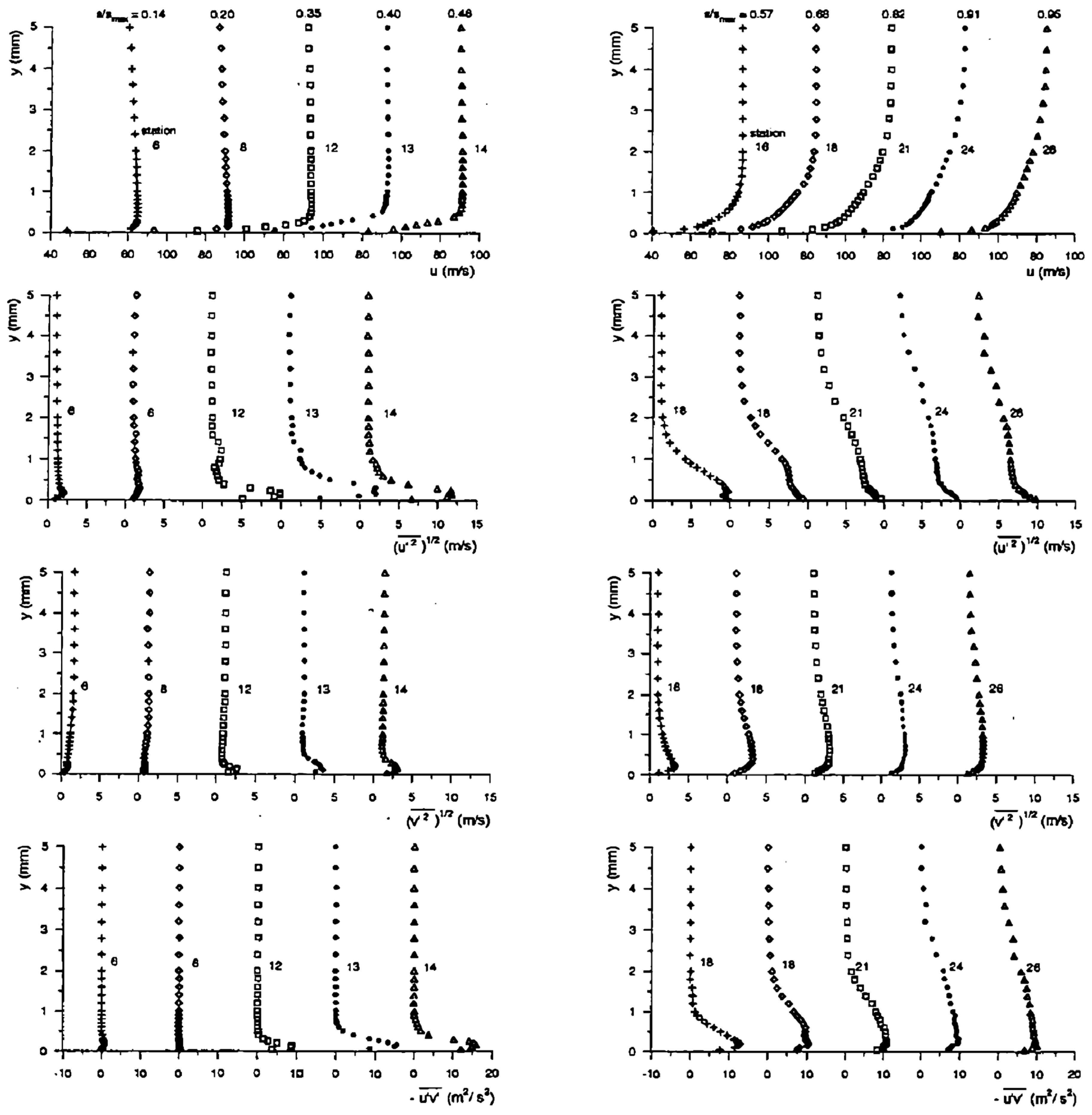
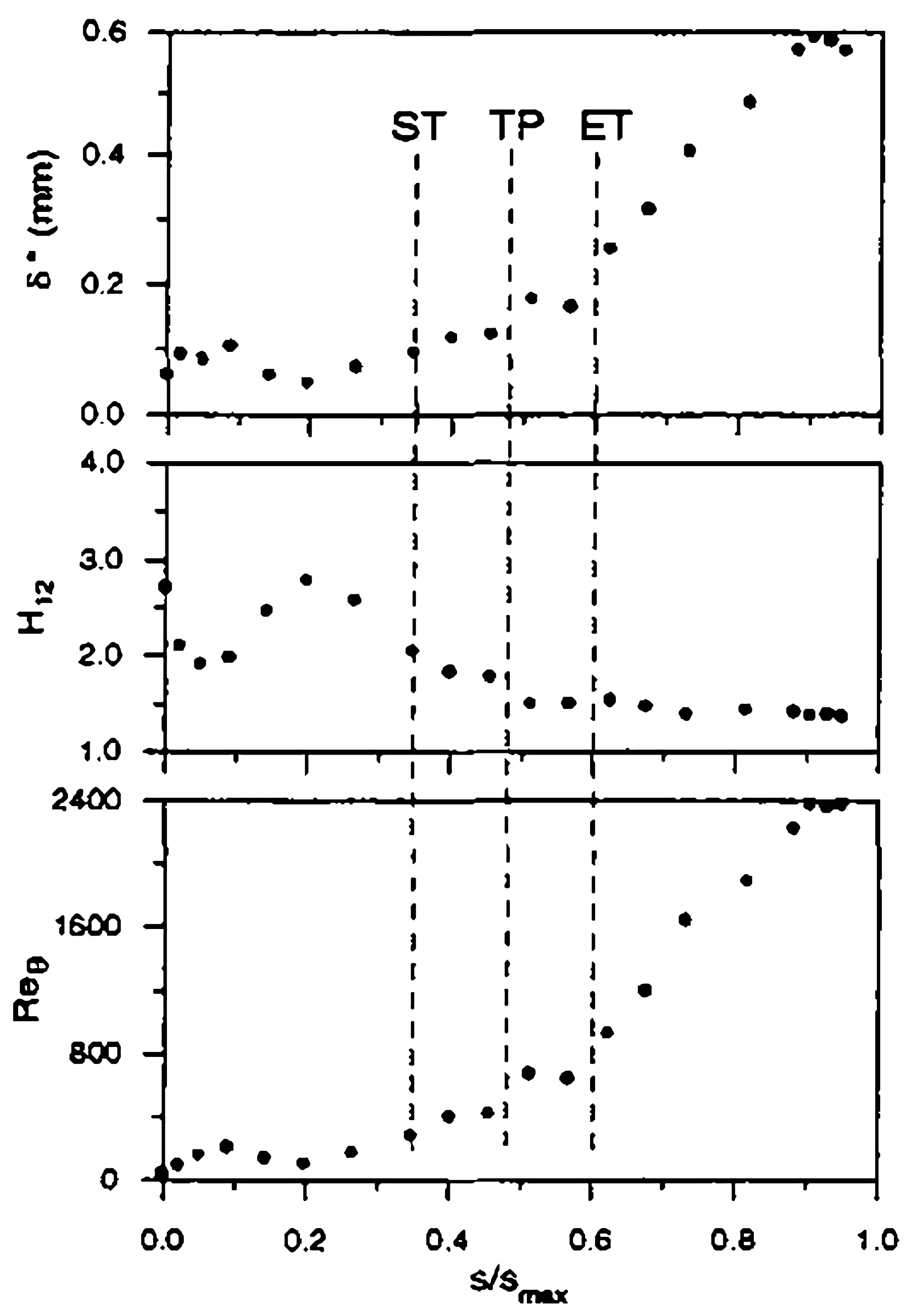
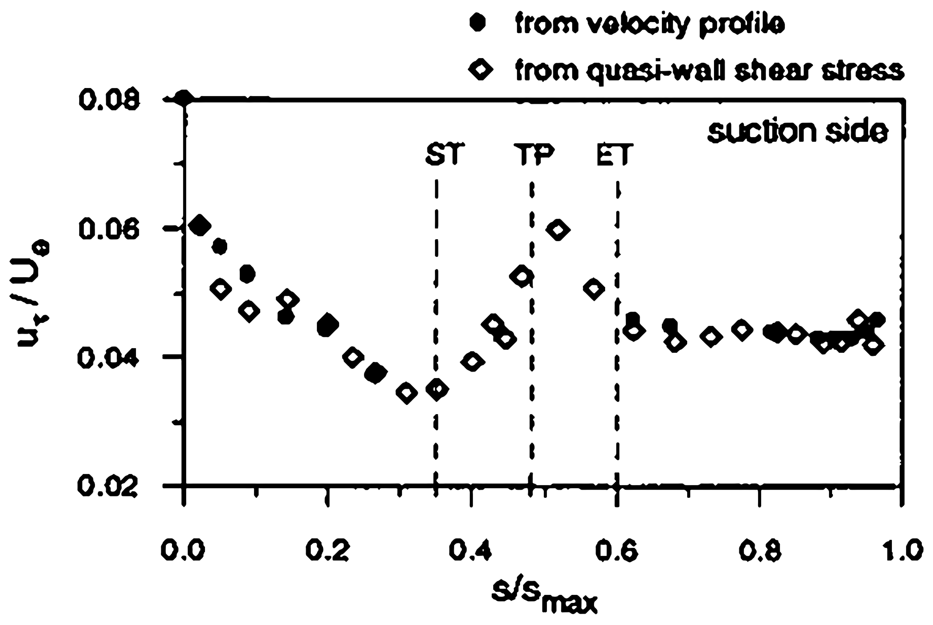
The experiments were carried out by Ubaldi in the low speed wind tunnel of IMSE (Istituto di Macchine e Sistemi Energetici), which consists of a blow down continuous operating circuit with an open test section. A centrifugal blower driven by a 70 kW a.c. motor equipped with an electronic frequency converter supplies a flow rate of 9 m/s at the pressure of 4000 Pa, when the rotational speed is 1500 rpm. A contraction with area ratio 8.63 and mesh screens of appropriate characteristics provide a low turbulence uniform flow in the 500 × 300 mm test section (Tu based on the streamwise fluctuations). A four-beam two-color fiber optic Laser Doppler Velocimetry (LDV) system with back-scatter collection optics (Dantec Fiber Flow) has been used to investigate the flow in the blade boundary layer. The light source is a 300 mW argon ion laser operating at 488 nm (blue) and 514.5 nm (green). The boundary layer mean velocity profiles (Figure A1) were measured by means of LDV and were used to evaluate boundary layer integral parameters, such as displacement thickness , shape factor , momentum thickness Reynolds number , and wall friction velocity , shown in Figure A2 and Figure A3.
Figure A1.
Boundary layer profiles of mean velocity and Reynolds stress components; (left): forward blade suction side; (right): rear blade suction side.
Figure A1.
Boundary layer profiles of mean velocity and Reynolds stress components; (left): forward blade suction side; (right): rear blade suction side.

Figure A2.
Boundary layer integral parameters on the blade suction side.

Figure A3.
Wall friction velocity distributions on the blade suction side.

Appendix A.2. Independence Study of Division of Train-Set and Test-Set
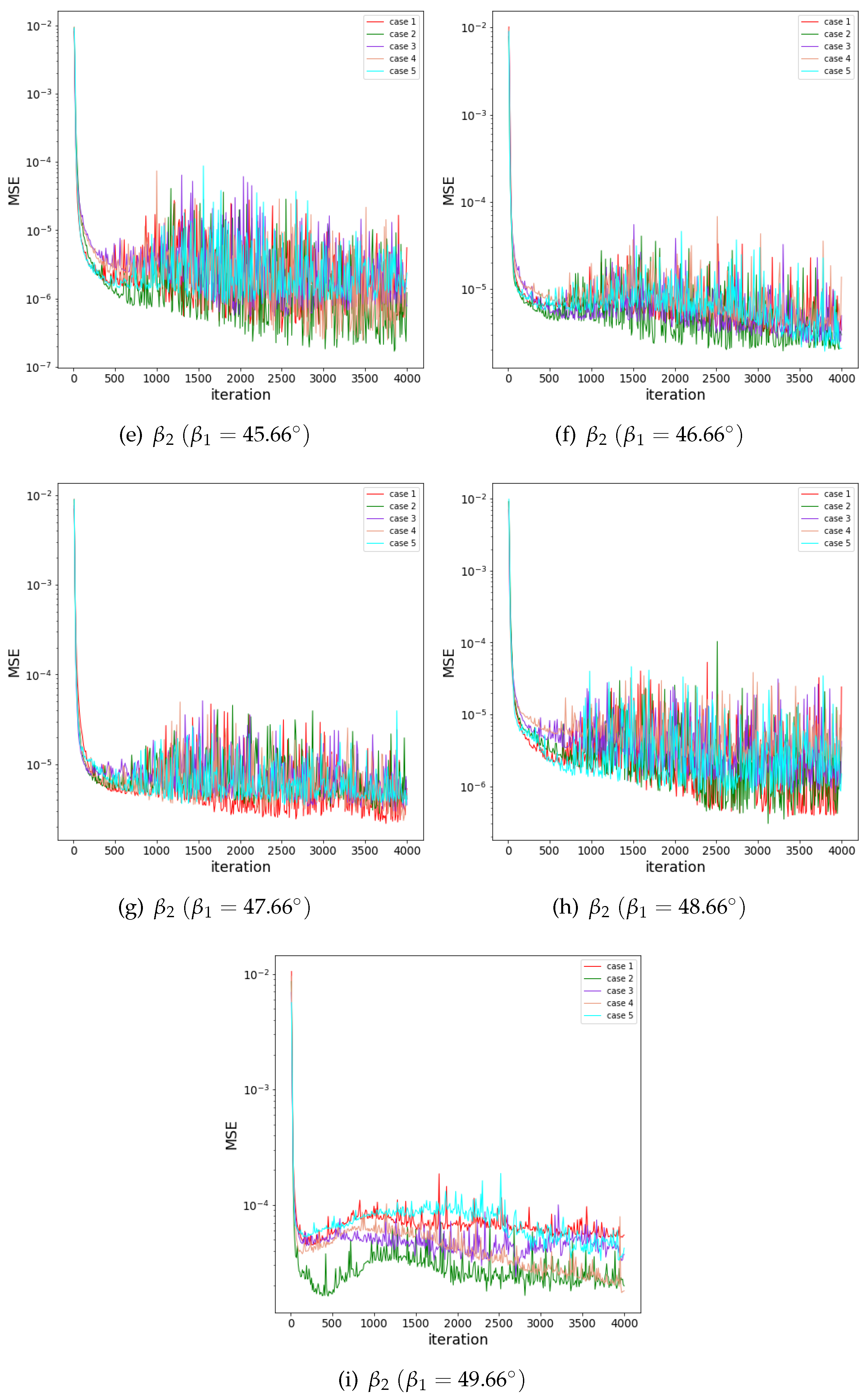
The ANN convergence curves of cases with different divisions of train-set and test-set are shown in Figure A4. The independence of training result on division of train-set and test-set can be proved.
Figure A4.
ANNconvergence curves of caseswith different divisions of train-set and test-set.


References
- Abbas, A.; de Vicente, J.; Valero, E. Aerodynamic technologies to improve aircraft performance. Aerosp. Sci. Technol. 2013, 28, 100–132. [Google Scholar] [CrossRef]
- Bushnell, D.M. Aircraft drag reduction—A review. Proc. Inst. Mech. Eng. Part J. Aerosp. Eng. 2003, 217, 1–18. [Google Scholar] [CrossRef]
- Li, Z.; Zheng, X. Review of design optimization methods for turbomachinery aerodynamics. Prog. Aerosp. Sci. 2017, 93, 1–23. [Google Scholar] [CrossRef]
- Marler, R.T.; Arora, J.S. Survey of multi-objective optimization methods for engineering. Struct. Multidiscip. Optim. 2004, 26, 369–395. [Google Scholar] [CrossRef]
- Jameson, A. Aerodynamic design via control theory. J. Sci. Comput. 1988, 3, 233–260. [Google Scholar] [CrossRef] [Green Version]
- Jameson, A.; Martinelli, L.; Pierce, N.A. Optimum Aerodynamic Design Using the Navier–Stokes Equations. Theor. Comput. Fluid Dyn. 1998, 10, 213–237. [Google Scholar] [CrossRef] [Green Version]
- Nielsen, E.J.; Anderson, W.K. Aerodynamic Design Optimization on Unstructured Meshes Using the Navier-Stokes Equations. AIAA J. 1999, 37, 1411–1419. [Google Scholar] [CrossRef] [Green Version]
- Luo, J.; Xiong, J.; Liu, F.; McBean, I. Three-Dimensional Aerodynamic Design Optimization of a Turbine Blade by Using an Adjoint Method. In Turbo Expo: Power for Land, Sea, and Air; ASME: New York, NY, USA, 2009; pp. 651–664. [Google Scholar]
- Marta, A.C.; Shankaran, S.; Wang, Q.; Venugopal, P. Interpretation of Adjoint Solutions for Turbomachinery Flows. AIAA J. 2013, 51, 1733–1744. [Google Scholar] [CrossRef]
- Luo, J.; Liu, F. Multi-Objective Optimization of a Transonic Compressor Rotor by Using an Adjoint Method. AIAA J. 2014, 53, 797–801. [Google Scholar] [CrossRef] [Green Version]
- Skinner, S.N.; Zare-Behtash, H. State-of-the-art in aerodynamic shape optimisation methods. Appl. Soft Comput. 2018, 62, 933–962. [Google Scholar] [CrossRef]
- Eberhart, R.; Kennedy, J. A new optimizer using particle swarm theory. In Proceedings of the MHS’95, Sixth International Symposium on Micro Machine and Human Science, Nagoya, Japan, 4–6 October 1995; pp. 39–43. [Google Scholar]
- Kirkpatrick, S.; Gelatt, C.D.; Vecchi, M.P. Optimization by Simulated Annealing. In Readings in Computer Vision; Fischler, M.A., Firschein, O., Eds.; Morgan Kaufmann: San Francisco, CA, USA, 1987; pp. 606–615. [Google Scholar] [CrossRef]
- Deb, K.; Pratap, A.; Agarwal, S.; Meyarivan, T. A fast and elitist multiobjective genetic algorithm: NSGA-II. IEEE Trans. Evol. Comput. 2002, 6, 182–197. [Google Scholar] [CrossRef] [Green Version]
- Goldberg, D.E. Genetic and evolutionary algorithms come of age. Commun. ACM 1994, 37, 113–119. [Google Scholar] [CrossRef]
- Fonseca, C.M.; Fleming, P.J. Genetic Algorithms for Multiobjective Optimization: FormulationDiscussion and Generalization. In Proceedings of the 5th International Conference on Genetic Algorithms, Urbana-Champaign, Champaign, IL, USA, 17–21 June 1993; pp. 416–423. [Google Scholar]
- Poloni, C.; Giurgevich, A.; Onesti, L.; Pediroda, V. Hybridization of a multi-objective genetic algorithm, a neural network and a classical optimizer for a complex design problem in fluid dynamics. Comput. Methods Appl. Mech. Eng. 2000, 186, 403–420. [Google Scholar] [CrossRef]
- Yang, Y.R.; Jung, S.K.; Cho, T.H.; Myong, R.S. Aerodynamic Shape Optimization System of a Canard-Controlled Missile Using Trajectory-Dependent Aerodynamic Coefficients. J. Spacecr. Rocket. 2012, 49, 243–249. [Google Scholar] [CrossRef]
- Tao, J.; Sun, G.; Si, J.; Wang, Z. A robust design for a winglet based on NURBS-FFD method and PSO algorithm. Aerosp. Sci. Technol. 2017, 70, 568–577. [Google Scholar] [CrossRef]
- Hilbert, R.; Janiga, G.; Baron, R.; Thévenin, D. Multi-objective shape optimization of a heat exchanger using parallel genetic algorithms. Int. J. Heat Mass Transf. 2006, 49, 2567–2577. [Google Scholar] [CrossRef]
- Samad, A.; Kim, K.Y. Shape optimization of an axial compressor blade by multi-objective genetic algorithm. Proc. Inst. Mech. Eng. Part J. Power Energy 2008, 222, 599–611. [Google Scholar] [CrossRef]
- Ju, Y.P.; Zhang, C.H. Multi-point and multi-objective optimization design method for industrial axial compressor cascades. Proc. Inst. Mech. Eng. Part J. Mech. Eng. Sci. 2011, 225, 1481–1493. [Google Scholar] [CrossRef]
- Benini, E. Three-Dimensional Multi-Objective Design Optimization of a Transonic Compressor Rotor. J. Propuls. Power 2004, 20, 559–565. [Google Scholar] [CrossRef]
- Oyama, A.; Liou, M.-S.; Obayashi, S. Transonic Axial-Flow Blade Optimization: Evolutionary Algorithms/Three-Dimensional Navier-Stokes Solver. J. Propuls. Power 2004, 20, 612–619. [Google Scholar] [CrossRef] [Green Version]
- Lian, Y.; Liou, M.-S. Multiobjective Optimization Using Coupled Response Surface Model and Evolutionary Algorithm. AIAA J. 2005, 43, 1316–1325. [Google Scholar] [CrossRef]
- Watkins, C.J.; Dayan, P. Q-learning. Mach. Learn. 1992, 8, 279–292. [Google Scholar] [CrossRef]
- Rabault, J.; Ren, F.; Zhang, W.; Tang, H.; Xu, H. Deep reinforcement learning in fluid mechanics: A promising method for both active flow control and shape optimization. J. Hydrodyn. 2020, 32, 234–246. [Google Scholar] [CrossRef]
- Viquerat, J.; Rabault, J.; Kuhnle, A.; Ghraieb, H.; Hachem, E. Direct Shape Optimization through Deep Reinforcement Learning. ResearchGate 2019. [Google Scholar] [CrossRef]
- Li, R.; Zhang, Y.; Chen, H. Learning the aerodynamic design of supercritical airfoils through deep reinforcement learning. arXiv 2020, arXiv:2010.03651. [Google Scholar]
- Mnih, V.; Kavukcuoglu, K.; Silver, D.; Rusu, A.A.; Veness, J.; Bellemare, M.G.; Graves, A.; Riedmiller, M.; Fidjeland, A.K.; Ostrovski, G.; et al. Human-level control through deep reinforcement learning. Nature 2015, 518, 529–533. [Google Scholar] [CrossRef]
- Silver, D.; Lever, G.; Heess, N.; Degris, T.; Wierstra, D.; Riedmiller, M. Deterministic policy gradient algorithms. In Proceedings of the 31st International Conference on International Conference on Machine Learning, Beijing, China, 21–26 June 2014; Volume 32, pp. I–387–I–395. [Google Scholar]
- Lillicrap, T.; Hunt, J.; Pritzel, A.; Heess, N.; Erez, T.; Tassa, Y.; Silver, D.; Wierstra, D. Continuous control with deep reinforcement learning. In Proceedings of the CoRR 2015, Tokyo, Japan, 12–14 March 2015. [Google Scholar]
- Yan, X.H.; Zhu, J.H.; Kuang, M.; Wang, X.Y. Aerodynamic shape optimization using a novel optimizer based on machine learning techniques. Aerosp. Sci. Technol. 2019, 86, 826–835. [Google Scholar] [CrossRef]
- Sun, G.; Wang, S. A review of the artificial neural network surrogate modeling in aerodynamic design. Proc. Inst. Mech. Eng. Part J. Aerosp. Eng. 2019, 233, 5863–5872. [Google Scholar] [CrossRef]
- Wang, S.Y.; Wang, C.; Sun, G. The Objective Space and the Formulation of Design Requirement in Natural Laminar Flow Optimization. Appl. Sci. 2020, 10, 5943. [Google Scholar] [CrossRef]
- Spalart, P.; Allmaras, S. A one-equation turbulence model for aerodynamic flows. In Proceedings of the 30th Aerospace Sciences Meeting and Exhibit, Reno, NV, USA, 6–9 January 1992. [Google Scholar] [CrossRef]
- Ning, F.; Xu, L. Numerical Investigation of Transonic Compressor Rotor Flow Using an Implicit 3D Flow Solver With One-Equation Spalart-Allmaras Turbulence Model. In Turbo Expo: Power for Land, Sea, and Air; American Society of Mechanical Engineers: New York, NY, USA, 2001; Volume 78507. [Google Scholar]
- Borm, O.; Danner, F. Numerical Optimization of Compressor Casing Treatments for Influencing the Tip Gap Vortex. In High Performance Computing in Science and Engineering, Garching/Munich 2007; Springer: Berlin/Heidelberg, Germany, 2009; pp. 215–225. [Google Scholar]
- Han, S.; Zhong, J. Effect of blade tip winglet on the performance of a highly loaded transonic compressor rotor. Chin. J. Aeronaut. 2016, 29, 653–661. [Google Scholar] [CrossRef] [Green Version]
- Lu, H.; Li, Q.; Pan, T. Optimization of cantilevered stators in an industrial multistage compressor to improve efficiency. Energy 2016, 106, 590–601. [Google Scholar] [CrossRef]
- Ma, W.; Ottavy, X.; Lu, L.; Leboeuf, F.; Gao, F. Experimental Study of Corner Stall in a Linear Compressor Cascade. Chin. J. Aeronaut. 2011, 24, 235–242. [Google Scholar] [CrossRef]
- Liu, Y.; Yan, H.; Liu, Y.; Lu, L.; Li, Q. Numerical study of corner separation in a linear compressor cascade using various turbulence models. Chin. J. Aeronaut. 2016, 29, 639–652. [Google Scholar] [CrossRef] [Green Version]
- Abu-Ghannam, B.J.; Shaw, R. Natural Transition of Boundary Layers—The Effects of Turbulence, Pressure Gradient, and Flow History. J. Mech. Eng. Sci. 1980, 22, 213–228. [Google Scholar] [CrossRef]
- Tucker, P.G. Trends in turbomachinery turbulence treatments. Prog. Aerosp. Sci. 2013, 63, 1–32. [Google Scholar] [CrossRef]
- Dick, E.; Kubacki, S. Transition Models for Turbomachinery Boundary Layer Flows: A Review. Int. J. Turbomach. Propuls. Power 2017, 2, 4. [Google Scholar] [CrossRef] [Green Version]
- Kožuloviş, D.; Röber, T.; Kügeler, E.; Nürnberger, D. Modifications of a two-equation turbulence model for turbomachinery fluid flows. In Proceedings of the Deutscher Luft- und Raumfahrtkongress, Dresden, Germany, 20 September 2004. [Google Scholar]
- Hu, J.; Fransson, T.; Hu, J.; Fransson, T. Transition predictions for turbomachinery flows using Navier-Stokes solver and experimental correlation. In Proceedings of the 15th Applied Aerodynamics Conference, Atlanta, GA, USA, 23–25 June 1997. [Google Scholar] [CrossRef]
- Sonoda, T.; Yamaguchi, Y.; Arima, T.; Olhofer, M.; Sendhoff, B.; Schreiber, H.-A. Advanced High Turning Compressor Airfoils for Low Reynolds Number Condition—Part I: Design and Optimization. J. Turbomach. 2004, 126, 350–359. [Google Scholar] [CrossRef]
- Yang, H.; Nuernberger, D.; Kersken, H.-P. Toward Excellence in Turbomachinery Computational Fluid Dynamics: A Hybrid Structured-Unstructured Reynolds-Averaged Navier-Stokes Solver. J. Turbomach. 2005, 128, 390–402. [Google Scholar] [CrossRef]
- Zhang, H.; Zou, Z.; Li, Y.; Ye, J.; Song, S. Conjugate heat transfer investigations of turbine vane based on transition models. Chin. J. Aeronaut. 2013, 26, 890–897. [Google Scholar] [CrossRef] [Green Version]
- Ubaldi, M.; Zunino, P.; Campora, U.; Ghiglione, A. Detailed Velocity and Turbulence Measurements of the Profile Boundary Layer in a Large Scale Turbine Cascade. In Proceedings of the ASME 1996 International Gas Turbine and Aeroengine Congress and Exhibition. Volume 1: Turbomachinery, Birmingham, UK, 10–13 June 1996. [Google Scholar]
- Queipo, N.V.; Haftka, R.T.; Shyy, W.; Goel, T.; Vaidyanathan, R.; Kevin Tucker, P. Surrogate-based analysis and optimization. Prog. Aerosp. Sci. 2005, 41, 1–28. [Google Scholar] [CrossRef] [Green Version]
- Yondo, R.; Andrés, E.; Valero, E. A review on design of experiments and surrogate models in aircraft real-time and many-query aerodynamic analyses. Prog. Aerosp. Sci. 2018, 96, 23–61. [Google Scholar] [CrossRef]
- Mengistu, T.; Ghaly, W. Aerodynamic optimization of turbomachinery blades using evolutionary methods and ANN-based surrogate models. Optim. Eng. 2008, 9, 239–255. [Google Scholar] [CrossRef]
- Ghalandari, M.; Ziamolki, A.; Mosavi, A.; Shamshirband, S.; Chau, K.W.; Bornassi, S. Aeromechanical optimization of first row compressor test stand blades using a hybrid machine learning model of genetic algorithm, artificial neural networks and design of experiments. Eng. Appl. Comp. Fluid. 2019, 13, 892–904. [Google Scholar] [CrossRef] [Green Version]
- Sun, G.; Sun, Y.J.; Wang, S.Y. Artificial neural network based inverse design: Airfoils and wings. Aerosp. Sci. Technol. 2015, 42, 415–428. [Google Scholar] [CrossRef]
- Goodfellow, I.; Bengio, Y.; Courville, A.; Bengio, Y. Deep Learning; MIT Press: Cambridge, UK, 2016; Volume 1. [Google Scholar]
- Kingma, D.P.; Ba, J. Adam: A method for stochastic optimization. arXiv 2014, arXiv:1412.6980. [Google Scholar]
- Sutton, R.; Barto, A. Reinforcement Learning: An Introduction; MIT Press: Cambridge, MA, USA, 1998. [Google Scholar]
- Hornik, K.; Stinchcombe, M.; White, H. Multilayer feedforward networks are universal approximators. Neural Netw. 1989, 2, 359–366. [Google Scholar] [CrossRef]
- Goecks, V.G.; Leal, P.B.; White, T.; Valasek, J.; Hartl, D.J. Control of Morphing Wing Shapes with Deep Reinforcement Learning. In Proceedings of the 2018 AIAA Information Systems-AIAA Infotech @ Aerospace, Kissimmee, FL, USA, 8–12 January 2018. [Google Scholar] [CrossRef]
- Xu, D.; Hui, Z.; Liu, Y.; Chen, G. Morphing control of a new bionic morphing UAV with deep reinforcement learning. Aerosp. Sci. Technol. 2019, 92, 232–243. [Google Scholar] [CrossRef]
- Moore, B. Principal component analysis in linear systems: Controllability, observability, and model reduction. IEEE Trans. Autom. Control. 1981, 26, 17–32. [Google Scholar] [CrossRef]
Figure 1.
Flowchart of multi-objective optimization of cascade blade profile.

Figure 2.
Shape functions of profile perturbation.

Figure 3.
Distribution of blade profiles perturbed by shape functions.

Figure 4.
VKI turbine blade profile.

Figure 5.
Computation grid of VKI cascade.

Figure 6.
The validation of transition position prediction. The scatters represent the distribution obtained from Ubaldi’s experiment [51]. The solid line represents the calculated intermittency factor distribution by computational fluid dynamics in this paper.
Figure 6.
The validation of transition position prediction. The scatters represent the distribution obtained from Ubaldi’s experiment [51]. The solid line represents the calculated intermittency factor distribution by computational fluid dynamics in this paper.

Figure 7.
Geometric shapes of initial cascade blades.

Figure 8.
An illustration of blade-to-blade topology.

Figure 9.
An illustration of computational grid of the cascade.

Figure 10.
Aerodynamic performance curves of the initial cascade.

Figure 11.
Computation results at different number of grid points.

Figure 12.
Structure of artificial neural network.

Figure 13.
Deep Deterministic Policy Gradient (DDPG) algorithm structure.

Figure 14.
Convergence curves of ANNs.

Figure 15.
The accumulative reward and objective function loss of each episode.

Figure 16.
Initial and optimized blade profiles: comparison in terms of shape.

Figure 17.
Aerodynamic performance curves of the cascades.

Figure 18.
distributions on suction and pressure surfaces.

Figure 19.
Absolute Mach number contours of initial and optimized blade profiles.


Table 1.
The range of bump function coefficients .
| 0.2 (SS) | −0.12 | 0.046 |
| 0.3 (SS) | 0 | 0.046 |
| 0.4 (SS) | 0.06 | 0.046 |
| 0.5 (SS) | 0.04 | 0.046 |
| 0.6 (SS) | 0 | 0.046 |
| 0.2 (PS) | −0.04 | 0.046 |
| 0.3 (PS) | −0.04 | 0.046 |
| 0.4 (PS) | −0.04 | 0.046 |
| 0.5 (PS) | −0.04 | 0.046 |
| 0.6 (PS) | −0.04 | 0.046 |
Table 2.
Geometric parameters of cascade.
| Parameter | Value |
|---|---|
| Chord length c (mm) | 109.5 |
| Solidity | |
| Blade geometric inlet angle () | 50.0 |
| Blade geometric outlet angle () | 11.4 |
| Blade camber angle () | |
| Blade stagger angle () |
Table 3.
Grid parameters.
| Block Name | Type | Points | Total Points |
|---|---|---|---|
| Inlet | H | 39,565 | |
| Up blade region | H | 104,545 | |
| Blade passage | O | 111,045 | |
| Down blade region | H | 104,545 | |
| Outlet | H | 47,765 | |
| Total | 407,465 |
Table 4.
The 1st and 2nd principal component of objective space analysis.
| 1st PC | −3.4 | 7.6 | −1.3 | 5.6 | −5.3 | 1.5 | 2.8 | 3.8 | −1.6 |
| 2nd PC | −4.1 | 5.7 | 3.9 | −6.9 | −1.2 | −2.4 | −3.0 | −3.0 | 6.8 |
Table 5.
Performance characteristics of the cascades at the operating point.
| initial | |||
| optimized |
Table 6.
Comparison of CFD simulation and ANN prediction on performance of the initial and optimized cascades.
Table 6.
Comparison of CFD simulation and ANN prediction on performance of the initial and optimized cascades.
| CFD simulation | ||||||
| ANN prediction |
Publisher’s Note: MDPI stays neutral with regard to jurisdictional claims in published maps and institutional affiliations. |
© 2020 by the authors. Licensee MDPI, Basel, Switzerland. This article is an open access article distributed under the terms and conditions of the Creative Commons Attribution (CC BY) license (http://creativecommons.org/licenses/by/4.0/).
Share and Cite
MDPI and ACS Style
Qin, S.; Wang, S.; Wang, L.; Wang, C.; Sun, G.; Zhong, Y. Multi-Objective Optimization of Cascade Blade Profile Based on Reinforcement Learning. Appl. Sci. 2021, 11, 106. https://0-doi-org.brum.beds.ac.uk/10.3390/app11010106
AMA Style
Qin S, Wang S, Wang L, Wang C, Sun G, Zhong Y. Multi-Objective Optimization of Cascade Blade Profile Based on Reinforcement Learning. Applied Sciences. 2021; 11(1):106. https://0-doi-org.brum.beds.ac.uk/10.3390/app11010106
Chicago/Turabian StyleQin, Sheng, Shuyue Wang, Liyue Wang, Cong Wang, Gang Sun, and Yongjian Zhong. 2021. "Multi-Objective Optimization of Cascade Blade Profile Based on Reinforcement Learning" Applied Sciences 11, no. 1: 106. https://0-doi-org.brum.beds.ac.uk/10.3390/app11010106
Note that from the first issue of 2016, this journal uses article numbers instead of page numbers. See further details here.