A Completion Method for Missing Concrete Dam Deformation Monitoring Data Pieces

Abstract

A concrete dam is an important water-retaining hydraulic structure that stops or restricts the flow of water or underground streams. It can be regarded as a constantly changing complex system. The deformation of a concrete dam can reflect its operation behaviors most directly among all the effect quantities. However, due to the change of the external environment, the failure of monitoring instruments, and the existence of human errors, the obtained deformation monitoring data usually miss pieces, and sometimes the missing pieces are so critical that the remaining data fail to fully reflect the actual deformation patterns. In this paper, the composition, characteristics, and contamination of the concrete dam deformation monitoring information are analyzed. From the single-value missing data completion method based on the nonlocal average method, a multi-value missing data completion method using BP (back propagation) mapping of spatial adjacent points is proposed to improve the accuracy of analysis and pattern prediction of concrete dam deformation behaviors. A case study is performed to validate the proposed method.

1. Introduction

1.1. Literature Reviews

A concrete dam can be regarded as a constantly changing complex system whose diverse and uncertain service behaviors are reflections to its special structure and working environment [1,2,3,4,5]. In operation status analyses of a concrete dam, the monitoring effect quantities such as deformation, seepage, stress, and strain can reflect the operation status patterns. Generally, deformation behaviors can show the operation status of the dam most directly [6,7,8,9,10]. A typical case is the Vaiont arch dam’s failure in Italy [11,12]. After the water storage was completed in 1960, the left front bank landslide of the dam slowly wriggled, and the measured total displacement reached 429 cm on 7 October 1963. Affected by the heavy rain on 9 October 1963, the dam broke, causing nearly 3000 deaths. The monitoring data showed that the displacement rate was 0.14 cm/d before the spring of 1963. After the continuous heavy rain on 18 September 1963, the displacement rate increased sharply from about 1 cm/d. The maximum velocity before the crash had reached 80 cm/d. So, it is significant to study the behaviors of a concrete dam.

The long lifetime of a concrete dam consequently accumulates a huge amount of deformation monitoring informative data for basic concrete dam deformation behavior analyses and predictions.

The effectiveness of the dam safety monitoring and evaluation can be reduced by the missing monitoring data pieces due to monitoring instrument failures or automatic monitoring instability. The data missing from the key-position monitoring instrument can impede the dam health monitoring processes. Therefore, it is of practical significance to study the missing data completion strategies in the case of monitoring instrument failure to provide a reliable decision basis for the safe dam operation.

The missing data completion has been applied to many fields [13,14,15,16]. In the field of dams, Lv et al. [17] pointed out that the interpolation methods of observation data mainly include internal physical association interpolation and mathematical interpolation and introduced the principle and process of linear interpolation. To obtain the homogenized data required by the model, Li et al. [18] compared the commonly used mathematical interpolation methods and chose the cubic Hermite piecewise interpolation with smooth interpolation curves that made full use of the existing data information to build the homogenized processing of the data sequence. To deal with the disadvantage of the “Runge Phenomenon” in the interpolation interval of the traditional interpolation function at both ends, Tu et al. [19] utilized the fractal interpolation in deducing the integrity state through partial information of the object to the interpolation calculation of missing time series, while the interpolation results were in line with expectations. Wang et al. [20] found that the same monitoring items such as a series of points on the deformation have a high degree of similarity and suggested combining the monitoring information of relevant measuring points. Firstly, the kernel independent component analysis algorithm was used to extract the independent components of relevant measurement points, and then the optimal characteristic variables were found by using eigenvalue spectrum analysis. Finally, an interpolation method for dam missing data based on KICA-RVM was established by using a relevance vector machine. Hu et al. [21] used the deformation information of the spatial adjacent points to return the deformation value of the target measurement points and proposed a spatial adjacent points regression interpolation method as well as a spatial anti-distance weighted interpolation method with good interpolation results. Other scholars also proposed spatial interpolation methods for dam deformation [22,23,24,25] and built a good foundation for in-depth analyses of dam deformation behaviors.

This paper analyzes the composition, characteristics, and contamination of the concrete dam deformation monitoring information. A multi-value missing data completion method using BP mapping of spatial adjacent points is proposed to improve the accuracy on analysis and pattern prediction of concrete dam deformation behaviors. The proposed method is validated by a case study.

1.2. Monitoring Data Characteristics

As an open system, a concrete dam has many factors and links that affect its deformation behaviors. These factors and links are the information sources of the concrete dam deformation monitoring. It can be seen from the composition of concrete dam deformation monitoring information in the previous section that the information sources have the following characteristics.

1.2.1. Multi-Systematic

The composition of a concrete dam is complex, which contains a large number of subsystems. The structure composition of a concrete dam includes the dam body, the dam foundation, and the dam near the reservoir area, and each represents a subsystem. Deformation monitoring can be divided into horizontal displacement monitoring, vertical displacement monitoring, crack opening monitoring, and each monitoring project can also be regarded as a subsystem. Different monitoring targets need different monitoring instruments to locate at different measuring points. Therefore, the monitoring information of the concrete dam deformation is multi-systematic.

1.2.2. Multi-Level

Different monitoring targets correspond to different monitoring methods, and in the concrete dam deformation monitoring system, the same monitoring project often contains different monitoring methods. Additionally, multiple measuring points are arranged in different parts of the dam, and the deformation behavior of the concrete dam is comprehensively reflected by measuring point information and different monitoring targets. Therefore, the monitoring information of the concrete dam deformation is multi-level.

1.2.3. Uncertainty

In the concrete dam deformation monitoring system, uncertainty arises since the interaction among the dam body, the dam foundation, and the monitoring system require different monitoring methods. The instrument precision variance, instrument performance degradation, and other factors also increase the uncertainty of the measured monitoring values [26,27]. In addition, the process of both manual and automatic monitoring can introduce errors and noises, which contributes to another source of uncertainty in monitoring data. Therefore, the monitoring information of the concrete dam deformation is uncertain.

1.3. Monitoring Data Contamination

From the characteristics of deformation monitoring information, it can be seen that the acquisition of concrete dam deformation information is affected by multiple factors. The information contamination is therefore inevitable and diverse, as shown in the following aspects:

(1)

Deficiency in information types

The deficiency in information types of concrete dam deformation monitoring data is objective and unavoidable. First of all, as a large engineering structure, a concrete dam occupies a large space system, the concrete dam deformation changes dynamically, and the distribution of the deformation changes is heterogeneous. Therefore, it is difficult to fully describe the deformation behaviors with existing methods and rules. Consequently, there exists a certain level of deficiency in monitoring information types. Secondly, the concrete dam deformation monitoring system monitors the deformation of the dam body intermittently, which means the system can only obtain sub-samples of some characteristic periods instead of real-time data for the dam deformation. The above situation also contributes to the deficiency in information types. Additionally, considering the applicability in engineering aspects, monitoring positions are usually arranged in typical locations to observe the deformation in a certain area. In this case, the deformation information of other locations in the same area is missing, which results in the deficiency in information types.

(2)

Incompleteness of a specific information type

In the process of monitoring the deformation of a concrete dam, the data collection from the automatic system is generally intermittent with a constant step size. For example, the monitoring instrument may perform one measurement every six hours or one measurement every day. However, due to human errors, instrument damage, data loss, and other factors in a manual monitoring system, the time interval between each monitoring point is not always the same, which will bring difficulties to the subsequent modeling work.

Particularly, in both automation and manual systems, sometimes because of equipment degradation, some monitoring information will be lost in a long sequence of measurement intervals. For example, a two-year data sequence may lose a continuous one-month or two-month period of data points due to equipment degradation, and if those measuring points are located in key positions, the monitoring system will fail to observe the abnormal deformation of the dam, which makes the dam safety analysis difficult. The long-period interruption of monitoring data can hinder the overall deformation analysis and future deformation prediction.

(3)

Errors in monitoring information

It can be seen from the monitoring methods of concrete dam deformation and the environmental influence factors that the deformation monitoring information cannot avoid errors. Generally, errors are divided into three groups—systematic errors, gross errors, and random errors. The expressions are as follows:

$$\epsilon ={\epsilon }_s+{\epsilon }_G+{\epsilon }_n$$

(1)

where, $\epsilon$ is the total error of observation, ${\epsilon }_s$ is the systematic error, ${\epsilon }_G$ is the gross error, and ${\epsilon }_n$ is the random error.

Systematic errors can be generated by intrinsic errors of the instrument, wrong measurement practices, environment changes, improper monitoring methods, imprecise theories, or formulary approximations. This type of error usually has a certain regularity. Researchers can assign a constant, a trend, or a period, to represent a systematic error in an analytic formula, curve, or number table.

In the process of obtaining, conveying, and processing deformation monitoring information, some data that are obviously inconsistent with the facts are sometimes produced. The errors generated by this type of data are called gross errors. In terms of numerical values, data whose absolute values are larger than two times the mean square errors can be regarded as gross errors, which are manifested as abnormal sudden jumps or outliers. The outliers are not representative enough for dam deformation characterizations, so they should be opted out from the deformation behavior analysis.

Random errors are errors that are caused by a combination of unrelated random factors. In the cases of a single measurement, the random errors may show no regularity in a single measurement, but with enough measurements, this type of error obeys the statistical laws. The noise is a kind of random error. The deformation monitoring information can be divided into real data information and noise information. In deformation behavior analysis and prediction, the existence of noise information will severely affect the accuracy of behavior analysis and prediction, so it is necessary to extract effective information from monitoring information.

2. Method

2.1. Completion Strategy for a Single Missing Value

2.1.1. Traditional Interpolation Completion Methods

For non-uniform time series with unequal time intervals, interpolation is usually used to homogenize them to satisfy the application requirements of building a statistical model. Frequently used interpolation methods include the piecewise linear interpolation, the nearest point interpolation, the cubic spline interpolation, and the cubic Hermite interpolation [18]. The principles of these methods are as follows:

(1)

Piecewise linear interpolation

Linear interpolation refers to the interpolation method whose interpolation function is a first-degree polynomial. The linear interpolation approximates the original function by using a line passing through two endpoints and estimating the missing data by plugging points located between these two endpoints. The method is simple and convenient. The piecewise linear interpolation is a simple linear interpolation between each short interval $\left[x_i,x_{i+1}\right]$, and the sub-interpolation polynomial on the interval $\left[x_i,x_{i+1}\right]$ is:

$$F_i=\frac{x-x_{i+1}}{x_i-x_{i+1}}f\left(x_i\right)+\frac{x-x_i}{x_{i+1}-x_i}f\left(x_{i+1}\right)$$

(2)

The interpolation function on the whole interval $\left[x_i,x_n\right]$ is:

$$F\left(x\right)={\displaystyle \sum _{i=1}^n{F}_i{l}_i\left(x\right)}$$

(3)

The definition of $l_i\left(x\right)$ is as follows:

$$l_i\left(x\right)=\{\begin{array}{cc}\frac{x-x_{i-1}}{x_i-x_{i-1}}& x\in \left[x_{i-1},x_i\right]\\ \frac{x-x_{i+1}}{x_i-x_{i+1}}& x\in \left[x_i,x_{i+1}\right]\\ 0& x\notin \left[x_{i-1},x_{i+1}\right]\end{array}$$

(4)

(2)

Nearest point interpolation

The nearest point interpolation estimates the function of the interpolation point by using the function of the nearest neighboring data point. This method is simple and intuitive, but the interpolation results are not so accurate.

Assuming the interpolation point is $\left(x_i,y_i\right)$, then:

$$y_i=y_{nearestx}$$

(5)

(3)

Cubic spline interpolation

The cubic spline interpolation, also called Spline interpolation for short, is an interpolation method to obtain the value of interpolation points by constructing a cubic spline interpolation function in the target interval. This method can effectively calculate the value of interpolation points and improve the smoothness of the interpolation curve. However, the computational cost of this interpolation is large.

Suppose there are interpolation nodes on the interval $\left[a,b\right]$, $a=x_1<x_2<\cdots <x_n=b$, and the corresponding function values are $y_1,y_2,\cdots ,y_n$. The cubic spline interpolation function $S\left(x\right)$ satisfies that $S\left(x_i\right)=y_i\left(i=1,2,\cdots ,n\right)$, and is not larger than the cubic polynomial value on the interval $\left[x_i,x_{i+1}\right]$, and it has a second continuous derivative on the interval $\left[a,b\right]$. Suppose the cubic polynomial on each subinterval $\left[x_i,x_{i+1}\right]$ is:

$$S_i\left(x\right)=a_i{x}^3+b_i{x}^2+c_{i}x+d_i,i=1,2,\cdots ,n-1$$

(6)

The function $S\left(x\right)$ needs to meet:

$$S\left(x_i\right)=y_i,S\left(x_i-0\right)=S\left(x_i+0\right),i=2,3,\cdots n-1$$

(7)

$$S^{\prime }\left(x_i-0\right)=S^{\prime }\left(x_i+0\right),S^{″}\left(x_i-0\right)=S^{″}\left(x_i+0\right),i=2,3,\cdots n-1$$

(8)

The expression of $S\left(x\right)$ can be obtained from a fixed boundary condition:

$$\begin{array}{ll}S\left(x\right)=& \frac{{\left(x_{i+1}-x\right)}^3}{6h_i}{M}_i+\frac{{\left(x-x_i\right)}^3}{6h_i}{M}_{i+1}+\left(y_i-\frac{M_i}{6}{h}_i^2\right)\frac{x_{i+1}-x}{h_i}+\\ & \left(y_{i+1}-\frac{M_{i+1}}{6}{h}_i^2\right)\frac{x-x_i}{h_i}\end{array}$$

(9)

where $h_i=x_{i+1}-x_i$; $M_i=S^{″}\left(x_i\right)$; $M_{i+1}=S^{″}\left(x_{i+1}\right)$.

By solving Equation (9) to get the parameters in Equation (8), the interpolation function on the interval $\left[a,b\right]$ can be constructed.

$$\left[\begin{array}{ccccc}2& 1& & & \\ {\mu }_2& 2& {\gamma }_2& & \\ & \ddots & \ddots & \ddots & \\ & & {\mu }_{n-1}& 2& {\gamma }_{n-1}\\ & & & {\mu }_n& 2\end{array}\right]\left[\begin{array}{c}{M}_1\\ M_2\\ ⋮\\ M_{n-1}\\ M_n\end{array}\right]=\left[\begin{array}{c}{\beta }_1\\ d_2\\ ⋮\\ d_{n-1}\\ {\beta }_n\end{array}\right]$$

(10)

where ${\gamma }_i=1-{\mu }_i$, ${\mu }_i=\frac{h_{i-1}}{h_{i-1}+h_i}$, $d_i=6\left(\frac{y_{i+1}-y_i}{h_i}-\frac{y_i-y_{i-1}}{h_{i-1}}\right)\frac{1}{h_{i-1}+h_i}$, ${\beta }_1=\frac{6}{h_1}\left(\frac{y_2-y_1}{h_1}-{y^{\prime }}_1\right)$, ${\beta }_n=\frac{6}{h_{n-1}}\left({y^{\prime }}_n-\frac{y_n-y_{n-1}}{h_{n-1}}\right)$.

(4)

Cubic Hermite interpolation

The Hermite interpolation method uses a curve to approximate the objective function, which not only requires that the interpolation curve strictly passes through the data points, but also needs to satisfy that the derivative value of each order at the data points is equal to the original function, to build a smooth interpolation curve. The cubic Hermite interpolation needs to know the function value of two nodes and the first derivative value to complete the construction. The algorithm is simple, and its interpolation results are close to real data, so it has been widely used.

Assuming that the two known nodes are $\left(x_{j-1},y_{j-1}\right)$ and $\left(x_j,y_j\right)$, and the corresponding first derivative values are ${y^{\prime }}_{j-1}$ and ${y^{\prime }}_j$, the interpolation polynomial $H_3\left(x\right)$ can be expressed as:

$$H_3\left(x\right)={\alpha }_{j-1}\left(x\right)y_{j-1}+{\alpha }_j\left(x\right)y_j+{\beta }_{j-1}\left(x\right){y^{\prime }}_{j-1}+{\beta }_j\left(x\right){y^{\prime }}_j$$

(11)

where ${\alpha }_{j-1}\left(x\right),{\alpha }_j\left(x\right),{\beta }_{j-1}\left(x\right),{\beta }_j\left(x\right)$ are the interpolation basis functions, and their highest degree cannot exceed 3.

$H_3\left(x\right)$ meets the conditions:

$$H_3\left(x_{j-1}\right)=y_{j-1},H_3\left(x_j\right)=y_j$$

(12)

$${H^{\prime }}_3\left(x_{j-1}\right)={y^{\prime }}_{j-1},{H^{\prime }}_3\left(x_j\right)={y^{\prime }}_j$$

(13)

Therefore, it can be solved by:

$${\alpha }_{j-1}\left(x\right)=\left(1+2\frac{x-x_{j-1}}{x_j-x_{j-1}}\right){\left(\frac{x-x_j}{x_j-x_{j-1}}\right)}^2$$

(14)

$${\alpha }_j\left(x\right)=\left(1-2\frac{x-x_j}{x_j-x_{j-1}}\right){\left(\frac{x-x_{j-1}}{x_j-x_{j-1}}\right)}^2$$

(15)

$${\beta }_{j-1}\left(x\right)=\left(x-x_{j-1}\right){\left(\frac{x-x_j}{x_j-x_{j-1}}\right)}^2,{\beta }_j\left(x\right)=\left(x-x_j\right){\left(\frac{x-x_{j-1}}{x_j-x_{j-1}}\right)}^2$$

(16)

Thus, the final expression can be obtained as:

$$\begin{array}{c}{H}_3\left(x\right)=\left(\left(1+2\frac{x-x_{j-1}}{x_j-x_{j-1}}\right)y_{j-1}+\left(x-x_{j-1}\right){y^{\prime }}_{j-1}\right){\left(\frac{x-x_j}{x_j-x_{j-1}}\right)}^2+\\ \left(\left(1-2\frac{x-x_j}{x_j-x_{j-1}}\right)y_j+\left(x-x_j\right){y^{\prime }}_j\right){\left(\frac{x-x_{j-1}}{x_j-x_{j-1}}\right)}^2\end{array}$$

(17)

The function parameters of the interpolation point can be obtained by substituting the x-coordinate at the interpolation point into Equation (17).

The rationality of the traditional interpolation method lies in that the approximation of a small part of missing data does not affect the overall trend and law of deformation time series. When the non-uniform data information is few, this kind of interpolation method can be used to cover up and generate deformation time series with equal intervals.

2.1.2. Single-Value Missing Data Completion Based on NLM (Non-local Means) Method

According to the function value or derivative value of the existing data points, the traditional interpolation method approximates the objective function by constructing a curve satisfying the basic conditions through certain mathematical methods, which can effectively solve the problem of time series inhomogeneity to a certain extent. However, these traditional interpolation methods are only based on known data and do not consider the physical significance of practical problems. The homogenization of the time series of non-uniform deformation is a supplement to the deformation information of the concrete dam at the unknown time point, which needs to take into account the actual deformation laws of the dam. On the other hand, in the actual deformation time series, the deformation values at different moments cannot be represented by precise functional expressions, so the derivative values of the data points cannot be obtained, and in this case, the traditional interpolation method is not applicable to solve the above problems.

In view of the situation that the time series have a long span and an uneven distribution, this paper adopts the non-local means method (NLM algorithm) [28] using non-local knowledge of deformation information and the self-similarity of information laws at different moments in the deformation sequence to estimate the deformation value at the missing time periods. On this basis, a complete deformation sequence having the strongest correlation with the deformation trend of the target is introduced as the calculation basis. The aim of this method is to characterize the missing information by considering the self-correlation between the deformation values at different moments of the deformation sequence and the correlation between the measurement points corresponding to the position of the target.

The main idea of the NLM algorithm is to obtain a new image by weighting and averaging the gray values of all pixels in the original image regarding the weight coefficients of similarity. In this paper, it is applied to the homogenization of concrete dam deformation time series to solve the single-value missing problem.

Assuming that the measured value of A deformation measurement point of the dam body is uneven, in order to estimate single missing data, the following steps are performed.

First, from the perspective of the whole deformation time series of the measuring points, find the measuring point B with the strongest correlation with the deformation trend of measuring point A and complete sequence. Measuring point B can be found from many measuring points on the same monitoring perpendicular line of point A. In this paper, the Pearson correlation test is adopted to calculate the correlations among deformation data of measurement points. Pearson correlation coefficient is a statistical parameter used to quantitatively measure the correlation between variables, and its calculation formula is:

$$r=\frac{N{\displaystyle \sum {\delta }_{1i}{\delta }_{2i}}-{\displaystyle \sum {\delta }_{1i}}{\displaystyle \sum {\delta }_{2i}}}{\sqrt{N{\displaystyle \sum {\delta }_{1i}^2}-{\left({\displaystyle \sum {\delta }_{1i}}\right)}^2}\sqrt{N{\displaystyle \sum {\delta }_{2i}^2}-{\left({\displaystyle \sum {\delta }_{2i}}\right)}^2}}$$

(18)

where ${\delta }_{1i}$ and ${\delta }_{2i}$ represent the deformation value of measuring points A and B at the same time, and N represents the total number of sequences.

It can be seen from Equation (18) that the value of Pearson’s correlation coefficient varies between −1 and 1, and the greater the absolute value of the correlation coefficient, the stronger the correlation between the two variables. When the correlation coefficient is closer to 1 or −1, the correlation is stronger, the closer the correlation coefficient to 0, the weaker the correlation. In addition, when the correlation coefficient is greater than 0, the two variables are positively correlated.

Secondly, the deformation value in the deformation time series of point B and the interpolation point in the sequence of point A at the same time can be referred to as the hypothesis interpolation point, and the weight of the deformation value of this hypothesis interpolation point at other points in the sequence of point B may be calculated. In this paper, the Square of Euclidean Distance (SED) is used to measure the similarity of deformation values at different times. The formula for calculating the square of Euclidean distance is:

$$d_{ij}\left(SED\right)={\left({\delta }_i-{\delta }_j\right)}^2$$

(19)

where ${\delta }_i$ and ${\delta }_j$ represent the deformation values corresponding to the measuring points at time $i$ and $j$.

In general, the smaller the difference is between the deformation values at different moments ${\delta }_{t_i}$ and ${\delta }_{t_j}$, the more similar the deformation is at the two moments, and the larger the weight value is given in the calculation. The weight is calculated by the following formula:

$$w\left(i,j\right)=\exp \left(-\frac{d_{ij}\left(SED\right)}{h^2}\right)$$

(20)

where h is the parameter that controls the increased or decreased speed of the exponential function and determines the weight.

Finally, calculate the weight of each reference point relative to the assumed interpolation point based on the complete deformation sequence of point B, and assign the deformation value to the measuring point A at the corresponding time. Then, the value of the interpolation point can be calculated by a weighted average. The formula is:

$${\delta }_i=\frac{{\displaystyle \sum _{j\in I}w\left(i,j\right){\delta }_j}}{{\displaystyle \sum _{j\in I}w\left(i,j\right)}}$$

(21)

where I represents the set of moments of the selected entire time series.

Assume the deformation time series of measuring points A and B are shown in Figure 1, where the sequence of measuring point B is complete, and there is a missing spot in the sequence of measuring point A. The dots in the figure represent the corresponding deformation values at different times, and the square point represents the missing value in the sequence of measuring points A, namely the interpolation point to be solved.

Point 1 in Figure 1 is a hypothetical interpolation point. Considering the similarity between other points and point 1 in the sequence, the deformation values of points 2, 3, and 4 are the same as that of point 1. According to the definition of Euclidean distance square, the weight of points 2, 3, and 4 is 1, and the closer the value is to the value of point 1, the larger the weight value is assigned. Through traversing the whole time series, the weight value of all points can be obtained. The weight value of each point in the B sequence is assigned to the corresponding point (points at the same time) in the A sequence, and the value of the interpolation points can be obtained after weighted averaging.

2.2. Completion Strategy for Multi Missing Values

When more information spots are missing in the deformation time series, the traditional interpolation method is not able to carry out effective interpolation calculation. Even though the NLM interpolation algorithm can calculate the value of each missing point, it needs to calculate the weight of existing points in the reference sequence to the missing points one by one, and then calculate the weight of each missing point in the target sequence. Although this method is feasible, the computational workload is large. To solve the above problem, this paper introduces a multi-value missing processing method and proposes a multi-value data missing completion method based on spatial adjacent point BP mapping.

2.2.1. Nonlinear Regression Analysis

The regression analysis studies the influence the degree of one variable to the other and estimates or predicts other variables’ changes. However, in practice, the changes of most variables are not one variable- but multi-variable-dependent. Moreover, the relation between the explained variables and many explanatory variables, such as the concrete dam deformation, is non-linear. According to the theory of the statistical model, the concrete dam deformation is mainly affected by three components—water pressure, temperature, and time effect. Each component includes more than one influence factor, so it is a multivariable nonlinear regression problem. The statistical model uses several factors to fit the deformation trend and obtains the multiple regression equation of deformation. Therefore, when a continuous multi-value is missing in the deformation time series of a certain measuring point, with known environmental quantity data, the regression relationship between the two can be established from known values in the sequence. The expression of the multivariable nonlinear regression analysis model is:

$${\delta }_t=f\left({\varphi }_1,{\varphi }_2,\cdots ,{\varphi }_n\right)+\epsilon$$

(22)

where $f$ represents the general function between ${\delta }_t$ and the influence factor, and ${\varphi }_i$ is the influence factor of concrete dam deformation.

After the equation between the deformation value and its influence factor is established, according to the measured data, the coefficients of each factor in the model can be determined by the least square method, and the multiple regression model is thus established. The value of missing information can be obtained by substituting the influence factor data of missing information segments into the above expression.

Given that the statistical model is established based on statistical methods and combined with dam theory, when the monitoring data sequence is long, if the factors in the statistical model are representative, the model can accurately reflect the deformation trend of concrete dams. Therefore, the multivariable nonlinear regression analysis model has been widely recognized in the dam construction field.

2.2.2. Spatial Adjacent Point Regression

When the fitting accuracy of the regression model to the deformation sequence is low or the environmental variables of the missing segment are unknown, the accuracy of the above completion method is low. Since the single section of concrete gravity dam and the whole dam body of concrete arch dam can be regarded as a whole, the deformation is naturally integrated and coherent, so the deformation in local areas is correlated to a certain extent. In other words, the missing information of a target measurement point can be estimated according to the deformation value of its adjacent measurement point.

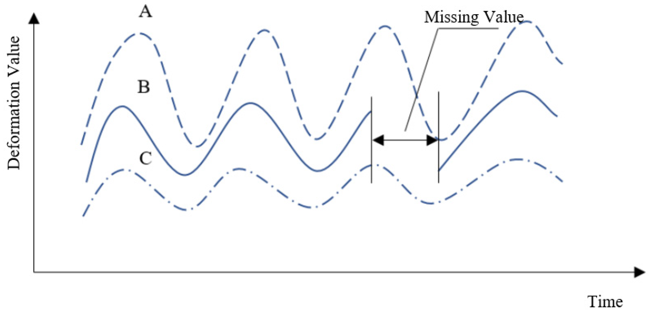
Assume that there are three monitoring points, A, B, and C, with similar locations and structures in the local area of a specific concrete dam section. The deformation sequences of measuring points A and C are complete, and a partial sequence of measuring point B is missing, as shown in Figure 2.

Considering the correlation of dam deformation at measuring points A, B, and C, there is a certain correlation between the deformation value of measuring point B and the deformation value of measuring points A and C. Therefore, according to the modeling idea of the statistical model, this paper takes the deformation value of measuring points A and C as the influence factors, and the deformation value of measuring point B as the target output to establish the correlation between measuring point B and measuring points A and C. The expression is:

$${\delta }_B=f\left({\delta }_A,{\delta }_C\right)+\epsilon$$

(23)

where $f\left({\delta }_A,{\delta }_C\right)$ represents the general function between ${\delta }_B$ and two influence factors, ${\delta }_A$, ${\delta }_C$, and the function relation can be expressed by polynomial as:

$${\delta }_B={\displaystyle \sum _{i=1}^{K_A}{\lambda }_{Ai}{\delta }_A^i}+{\displaystyle \sum _{i=1}^{K_C}{\lambda }_{Ci}{\delta }_C^i}+{\beta }_B+\epsilon$$

(24)

where ${\lambda }_{Ai}$ and ${\lambda }_{Ci}$ represent the coefficients of each polynomial of ${\delta }_A$ and ${\delta }_C$ respectively, $K_A$ and $K_C$ represent the highest order of ${\delta }_A$ and ${\delta }_C$, and ${\beta }_B$ is the translation term.

If Equation (24) is expanded, let the number of adjacent measurement points in the local area of the target measurement point be abstracted as L, then:

$${\delta }_{it}={\displaystyle \sum _{j=1}^L{\lambda }_{ij}f\left({\delta }_{jt}\right)}+{\beta }_i+\epsilon$$

(25)

where ${\delta }_{it}$ and ${\delta }_{jt}$ represent the deformation values of the measuring point i and the adjacent measuring point j at time t respectively, and ${\lambda }_{ij}$ represents the influence coefficient of each factor.

From the above analysis, with the known deformation information of the target measurement point and the adjacent measurement points, the least square method can also estimate the influence coefficients, and the expression of the model is thus established. By substituting the hypothesis missing information of the adjacent measurement point into Equation (25), the missing information of the target measurement point can be estimated.

2.2.3. BP Mapping of Spatial Adjacent Points

The spatial adjacent point regression interpolation method establishes the correlation between the deformation value of the target measurement point and the deformation value of the adjacent points, which can effectively reveal the relationships among the deformation values of the spatial adjacent measurement points. However, the measuring points that are located on the same deformation body, such as the measuring points on the same section of the concrete gravity dam and concrete arch dam, have integrity, correlations, mutual influences, and correlations in deformation, so the specific relationships between the deformation of these measuring points are complex. However, the spatial adjacent point regression method, which is based on the modeling idea of the statistical model, only regresses the power series expansion of finite integer terms of variables, so it is difficult to fully describe the unknown relationships between the deformation of measurement points, and therefore this regression method has limitations.

It is difficult to represent the complex and unknown relationship between the deformation of spatial measurement points by specific mathematical expressions. But the BP neural network, with strong nonlinear mapping ability, can delineate the complex information relationship behind the data through learning and training of samples. Meanwhile, the BP neural network also has strong generalization ability, so that the trained network can effectively process new input samples and give appropriate output results. Therefore, in order to improve the accuracy of the missing value completion and find the true value of deformation closest to the missing time, the BP neural network is introduced in this section to deal with the unknown relationship between the deformation of spatial measurement points. A corresponding missing value completion method is proposed.

The BP network is a kind of multi-layer feedforward neural network, which realizes operation through forward signal propagation and back error propagation. It has three layers: input layer, hidden layer, and output layer. Each layer is composed of nodes (namely neurons). The upper and lower nodes are connected by weight, and the nodes of the same layer are independent of each other. Through the connection weights between the upper and lower neurons, the network transforms the output of the upper neuron to the input of the lower neuron, thus realizing the learning calculation of the samples.

Assume that there are n monitoring points that are spatially adjacent and structurally related at a concrete dam body, such as points of a concrete gravity dam that are on the same vertical line or points within the same deformation zone of a concrete arch dam (partition method is not explained in detail in this paper), when the deformation information of the ith measuring point is missing due to some reasons, the known information of other m = n − 1 measuring points can be used to estimate the information of point $i$. The steps to establish a multi-value data missing completion method based on BP neural network mapping are as follows:

Suppose that the sample set contains Z pattern pairs between the input vector and the output vector, randomly select a pattern pair $k$, while the input pattern vector is $A_k=\left(a_1^k,a_2^k,\cdots ,a_m^k\right)$, and the expected output vector is $Y_k=\left(y_1^k\right)$. The input vector of the middle layer element is $S=\left(s_1,s_2,\cdots ,s_p\right)$ ($p$ is the number of hidden layer nodes, the same below), and the output vector is $B_k=\left(b_1,b_2,\cdots ,b_p\right)$. The input vector of the output layer element is $L_k=\left(l_1,l_2,\cdots ,l_p\right)$, and the output vector is $C=\left(c\right)$. The connection weight between the input layer and the hidden layer is $w\left(w=w_{ij},i=1,2,\cdots ,m;j=1,2,\cdots ,p\right)$. The connection weight between the hidden layer and the output layer is $v\left(v=v_j,j=1,2,\cdots ,p\right)$. The output threshold of each unit in the hidden layer is $\theta \left(\theta ={\theta }_j,j=1,2,\cdots ,p\right)$. The output threshold of the output layer unit is $\gamma =\left(\gamma \right)$.

(1) Network parameters are initialized by using random assignment functions to assign $w$, $v$, $\theta$, and $\gamma$ small random values between (−1,1).

(2) Input vector $A_k$, connection weight $w$, and threshold $\theta$ are used to calculate the input $S$ of the hidden layer. Calculate the output $B_k$ of the hidden layer through Sigmoid function with $S$, namely:

$$\begin{array}{cc}{s}_j={\displaystyle \sum _{i=1}^m{w}_{ij}{a}_i}-{\theta }_j& j=1,2,\cdots ,p\end{array}$$

(26)

$$\begin{array}{cc}{b}_j=f\left(s_j\right)& j=1,2,\cdots ,p\end{array}$$

(27)

$$f\left(x\right)=\frac{1}{1+e^{-x}}$$

(28)

(3) The output $B_k$, connection weight $v$, and threshold $\gamma$ of the hidden layer are used to calculate the input $L_k$ of the output layer element, and then the output vector $c$ of the output layer element is calculated with $L_k$, namely:

$$l={\displaystyle \sum _{j=1}^p{v}_j{b}_j}-\gamma$$

(29)

$$c=f\left(l\right)$$

(30)

(4) The expected output vector $Y_k$ and the actual network output $c$ are used to calculate the generalized error $d^k$ of the output layer element, namely:

$$d^k=\left(y^k-c\right)c\left(1-c\right)$$

(31)

(5) The connection weight $v$, the generalization error $d^k$ of the output layer, and the output $B_k$ of the hidden layer are used to calculate the generalization error $e^k$ of each element of the hidden layer, namely:

$$e_j^k=\left(d^k{v}_j\right)b_j\left(1-b_j\right)$$

(32)

(6) Use the generalized error $d^k$ of the output layer element and the output $B_k$ of each element in the middle layer to correct the connection weight $v$ and threshold $\gamma$, that is:

$$v_j\left(N+1\right)=v_j\left(N\right)+\eta d^k{b}_j+\alpha \left(v_j\left(N\right)-v_j\left(N-1\right)\right)$$

(33)

$$\gamma \left(N+1\right)=\gamma \left(N\right)+\eta d^k$$

(34)

where $\eta$ stands for learning efficiency and take $\eta =0.01~0.8$. $\alpha$ is the momentum factor and take $\alpha =0.9$.

(7) The connection weight $w$ and threshold $\theta$ are modified by the generalized error $e_j^k$ and input mode vector $A_k$ of each element of the hidden layer, namely:

$$w_{ij}\left(N+1\right)=w_{ij}\left(N\right)+\eta e_j^k{a}_i^k+\alpha \left(w_{ij}\left(N\right)-w_{ij}\left(N-1\right)\right)$$

(35)

$${\theta }_j\left(N+1\right)={\theta }_j\left(N\right)+\eta e_j^k$$

(36)

(8) Randomly select another learning pattern pair in the training sample set and repeat steps (3)–(6) until all pattern pairs are trained.

(9) Calculate the global error function $E$ of the network, and its formula is:

$$E={\displaystyle \sum _{k=1}^Z{E}_k}={\displaystyle \sum _{k=1}^Z{\left(y^k-c\right)}^2/2}$$

(37)

If $E$ is less than a preset error value, the network stops learning; otherwise, repeat steps (3)–(8) for the next round of learning and training of the sample set.

(10) The trained network is saved, while new samples are input, and the output result of missing information completion is obtained.

Take $n=5$ as an example, the input layer is the deformation sequence of four relevant measurement points, and the output layer is the deformation sequence of the target measurement points. The network structure is shown in Figure 3.

3. Case Study

In order to verify the feasibility and effectiveness of the incomplete information processing and gross error detection methods proposed in this chapter, the deformation data of a concrete gravity dam is used in this analysis.

This gravity dam is located at the junction of Yibin County, Sichuan Province, and Shuifu County, in Yunnan Province. The dam serves various purposes: power generation, improvement of navigation conditions, flood and sand control, and irrigation. The mountains on both sides of the dam toe incline slightly to the downstream. The bedrock surface of the dam (riverbed) is slightly inclined upstream, and there are coherent grooves on both sides. Bedrock lithology and lithofacies change abruptly, thus, the cross-stratification develops. Eleven small faults are found over the riverbed and dam foundation. The planform of the dam is shown in Figure 4.

This dam is a concrete gravity dam with a normal water level of 380.0 m and a dead water level of 370.0 m. The dam water-retaining structures include the sluice section, the non-overflow dam section, the sand flushing hole dam section, the ship lift dam section, the powerhouse dam section, and the water release dam section. The dam crest elevation is 384.0 m (above sea level), with maximum dam height of 162.0 m, and dam crest length of 909.26 m. The upstream vertical view of the dam is shown in Figure 5.

The average annual rainfall of the reservoir is 1000 mm, with the maximum level of the annual daily rainfall over 90 mm, or the medium annual daily rainfall level in the Sichuan Province. The upstream water level (recently) is 380 m and has remained high for a long time. The downstream water level is usually around 270 m.

In order to monitor the horizontal displacement of the dam, vertical lines are arranged in each important dam section. In this section, the monitoring data of each measuring point on the positive vertical line of the dam sluice Section 1 are taken as an example for analysis (Figure 6). The horizontal displacement process line of the six measuring points is shown in Figure 7. The frequency of measurement is once a day. It can be found that the horizontal displacement process line of these measuring points has strong correlation.

4. Result and Discussion

4.1. Single-Value Missing Data Completion

Take the measuring point PL5-3 in Figure 6 as an example, the strongest correlation reference sequence with the deformation sequence of the measuring point is searched. The correlation between the sequence of target measurement points and the sequence of other measurement points is shown in

Table 1. Correlation results of deformation sequences of target measurement points and adjacent measurement points.

Adjacent Points	PL5	PL5-1	PL5-2	PL5-4	PL5-5
Target Points
PL5-3	0.7952	0.9231	0.9563	0.9895	0.9668

.

It can be seen from the calculation results in the above table that the deformation sequence of measuring point PL5-4 has the strongest correlation with the target sequence, and the deformation law is the most similar. Therefore, the reference measuring point is PL5-4.

For the deformation sequence from 31 August 2014 to 18 September 2014, there are 19 deformation data point, as shown in

Table 2. Summary table of deformation data of target measurement points and reference measurement points.

Date	Deformation Value/mm		Date	Deformation Value/mm
	PL5-3	PL5-4		PL5-3	PL5-4
2014 August 31	6.14	6.85	2014 September 10	7.93	9.41
2014 September 1	6.18	7.09	2014 September 11	7.83	9.22
2014 September 2	6.84	7.75	2014 September 12	8.06	9.31
2014 September 3	6.93	7.95	2014 September 13	8.47	9.82
2014 September 4	7.98	9.20	2014 September 14	7.91	9.18
2014 September 5	8.38	9.63	2014 September 15	8.07	9.42
2014 September 6	8.10	9.62	2014 September 16	8.12	9.49
2014 September 7	8.36	9.66	2014 September 17	8.37	9.70
2014 September 8	7.74	9.21	2014 September 18	8.17	9.36
2014 September 9	7.88	9.13

.

Suppose that the deformation data of 10 September 2014 is missing, use the interpolation method based on non-local means proposed in this paper and the traditional method to estimate the missing value, respectively. The results are shown in

Table 3. Comparison of the estimated results of each interpolation method.

Missing True Value/mm	Estimates for Each Method/mm
	Linear Interpolation		Proximity Interpolation		Spline Interpolation		Hermite Interpolation		NLM Interpolation
	Value	Error	Value	Error	Value	Error	Value	Error	Value	Error
7.93	7.8550	0.075	7.8300	0.1	7.9175	0.0125	7.8556	0.0744	7.9316	0.0016

.

It can be seen from the calculation results of each interpolation method that the estimation result of the proposed single-value missing completion method based on non-local means is close to the original monitoring values. At the same time, it can be found that when the missing value is not within the range of two values before and after the missing value, the traditional interpolation method is difficult to estimate such deformation value effectively. However, the NLM interpolation method overcomes this limitation by using self-similarity of deformation sequences and introducing reference sequences, which increases the accuracy of missing value estimation.

4.2. Multi-Value Missing Data Completion

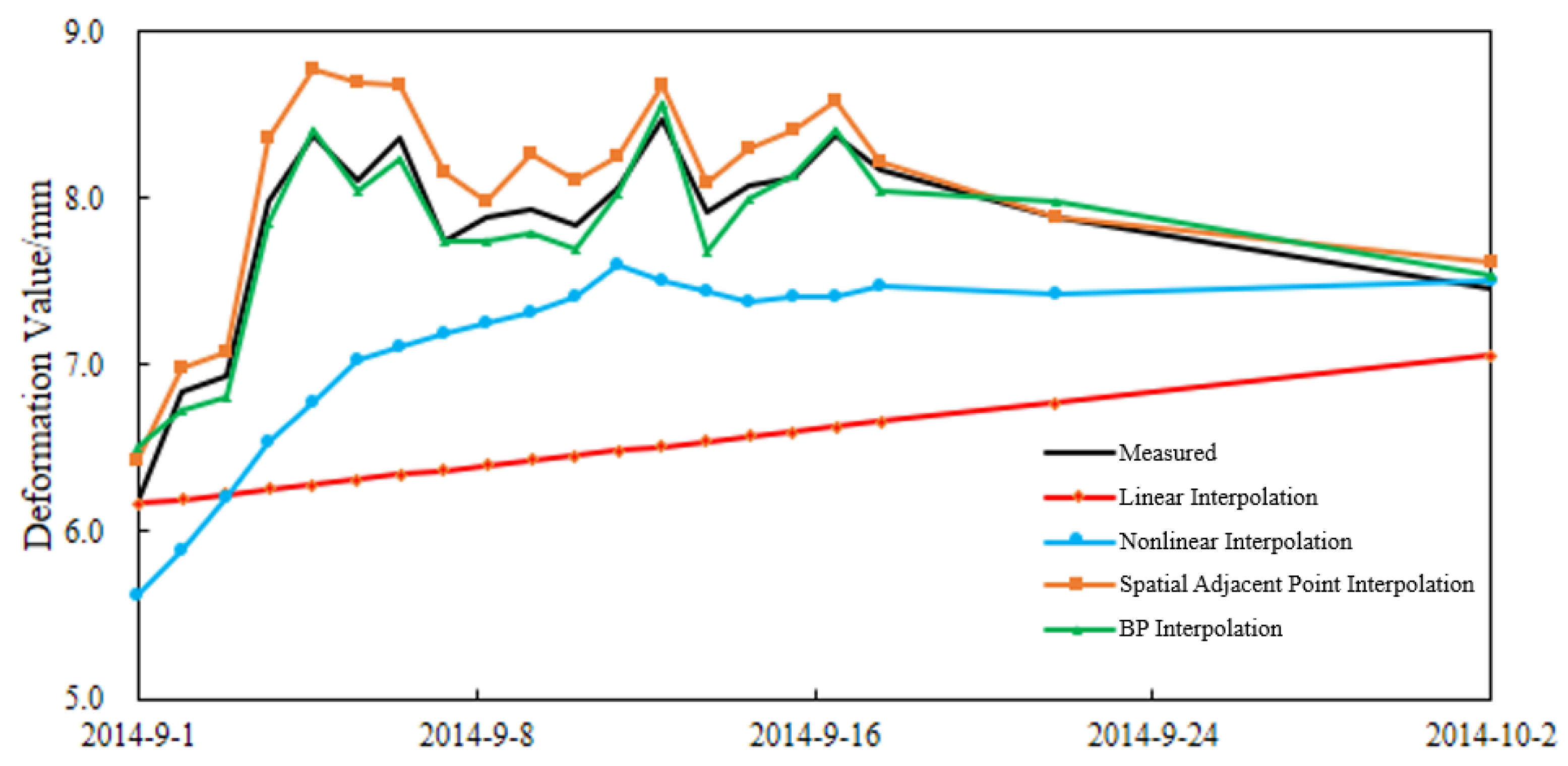
Similarly, take the deformation sequence of PL5-3 as an example. A one-month missing segment is constructed manually (from 1 September 2014 to 2 October 2014). The BP neural network is used to establish the mapping relationship between other measurement points on the same vertical line and the deformation sequence of target measurement points. First, the training samples made up of known deformation data of each measurement point are imported into the BP neural network for learning. Second, the deformation values of the missing time of other measurement points are constituted and imported into the trained network to calculate the missing data of target measurement points. The calculation results of each method are shown in Figure 8, and the completion accuracy is shown in

Table 4. Comparison of completion accuracy of missing values.

Completion Method	Linear Interpolation	Nonlinear Interpolation	Space Adjacent Points Interpolation	BP Interpolation
Determination coefficient	0.1094	0.6053	0.9518	0.9527
Root Mean Square error	1.4702	0.8470	0.2753	0.1292

.

As can be seen from the results in Figure 8 and Table 4, the completion accuracy of the multi-value missing completion method proposed in this paper based on spatial adjacent point BP mapping is higher than that of the other three methods. The coefficient of determination and root-mean-square error all achieve satisfactory results. The interpolation method of spatial adjacent points also has a good estimation result, but since this method only uses the deformation information of the upper and lower measurement points for regression analysis, it cannot fully dig out the relevant information of the deformation of the target measurement points. The nonlinear regression utilizes the idea of a statistical model, which can be used for completion under the condition of tiny changes of environment quantity. The effect of linear interpolation is poor, so it is difficult to estimate multi-value missing data.

5. Conclusions

This paper proposed a completion method for the missing deformation monitoring data of concrete dams. The main points are as follows:

(1)

The monitoring data missing of concrete dam deformation was discussed, including deformation monitoring data characteristics and data contamination types.

(2)

A data completion method with high accuracy, good stability, and strong adaptability validated through a case study was proposed. By reviewing the traditional processing methods to deal with incomplete information, this paper discussed the principle and weakness of traditional missing value completion methods in the case of single-value missing and multi-value missing. For the single-value missing in monitoring data, the non-local mean method was studied, and the regression interpolation method of spatial adjacent points was improved to accomplish data completion. For the multi-value missing data completion, the nonlinear regression and the spatial adjacent point regression were used, and the BP mapping of spatial adjacent points was proposed to complete the missing data pieces. The method proposed in this work is simple and effective to complete long data sequences and can meet the requirements of safety monitoring during dam operation.

References

- Zhu, S. History of Dam Technology; China Water & Power Press: Beijing, China, 1995. [Google Scholar]
- Feng, Y. Overview on operation safety management for hydropower dams. Dam Saf. 2017, 2017, 1–6. [Google Scholar]
- Zhang, X. Items and elements in assessment of operation safety of hydropower dams. Dam Saf. 2015, 2015, 5–8. [Google Scholar]
- Zhang, X. Collection of typical cases of dam failures and accidents at hydropower stations. Dam Saf. 2015, 2015, 13–16. [Google Scholar]
- Zhu, Y.; Niu, X.; Gu, C.; Yang, D.; Sun, Q.; Rodriguez, E.F. Using the DEMATEL-VIKOR Method in Dam Failure Path Identification. Int. J. Environ. Res. Public Health 2020, 17, 1480. [Google Scholar] [CrossRef] [PubMed] [Green Version]
- Ru, N.; Jiang, Z. Dam Accident and Safety Arch Dam; China Water & Power Press: Beijing, China, 1995. [Google Scholar]
- Pan, J. Thousand Years of Merits and Demerits of Dam; Tsinghua University Press: Beijing, China, 2000. [Google Scholar]
- Yang, B. Spatial and Temporal Characteristics Identification and Prediction Method of Dam Deformation Based on Measured Data. Ph.D. Thesis, Hohai University, Nanjing, China, 2017. [Google Scholar]
- Gu, H.; Yang, M.; Gu, C.; Cao, W.; Huang, X.; Su, H. An analytical approach of behavior change for concrete dam by panel data model. Steel Compos. Struct. 2020, 36, 521–531. [Google Scholar]
- Ge, W.; Wang, X.; Li, Z.; Zhang, H.; Guo, X.; Wang, T.; Gao, W.; Lin, C.; van Gelder, P. Interval analysis of loss of life caused by dam failure. J. Water Resour. Plan. Manag. 2021, 147, 04020098. [Google Scholar] [CrossRef]
- Chiara, D.V.; Giovanni, G.; Marco, B. Insights from analogue modelling into the deformation mechanism of the Vaiont landslide. Geomorphology 2015, 228, 52–59. [Google Scholar]
- Paolo, P.; Alberto, B. Gravity-induced rock mass damage related to large en masse rockslides: Evidence from Vajont. Geomorphology 2015, 234, 28–53. [Google Scholar]
- Li, Q.; Xu, Y. VS-GRU: A Variable Sensitive Gated Recurrent Neural Network for Multivariate Time Series with Massive Missing Values. Appl. Sci. 2019, 9, 3041. [Google Scholar] [CrossRef] [Green Version]
- Kim, T.; Ko, W.; Kim, J. Analysis and Impact Evaluation of Missing Data Imputation in Day-ahead PV Generation Forecasting. Appl. Sci. 2019, 9, 204. [Google Scholar] [CrossRef] [Green Version]
- Rodenburg, F.J.; Sawada, Y.; Hayashi, N. Improving RNN Performance by Modelling Informative Missingness with Combined Indicators. Appl. Sci. 2019, 9, 1623. [Google Scholar] [CrossRef] [Green Version]
- Choi, Y.-Y.; Shon, H.; Byon, Y.-J.; Kim, D.-K.; Kang, S. Enhanced Application of Principal Component Analysis in Machine Learning for Imputation of Missing Traffic Data. Appl. Sci. 2019, 9, 2149. [Google Scholar] [CrossRef] [Green Version]
- Lv, K. Research and Analysis about the Deformation Forecasting Methods of Yellow River Xiaolangdi Water Hydropower Dam. Ph.D. Thesis, China University of Mining and Technology, Beijing, China, 2012. [Google Scholar]
- Li, S.; Zhang, B. Forecast model for dam deformation based on wavelet and spectral analysis. Chin. J. Geotech. Eng. 2015, 37, 374–378. [Google Scholar]
- Tu, L.; Bao, T.; Li, Y. ARIMA Dam Early Warning Model Based on Fractal Interpolation. J. China Three Gorges Univ. Nat. Sci. 2015, 37, 29–32. [Google Scholar]
- Wang, J.; Dong, J.; Cheng, L. An interpolation method based on KICA-RVM for missing monitoring data of dam. J. Water Resour. Water Eng. 2017, 28, 197–201. [Google Scholar]
- Hu, T. Research on Spatiotemporal Data Mining Model of Concrete Dam Deformation; Hohai University: Nanjing, China, 2017. [Google Scholar]
- Liu, Q.; Deng, N. A Study of Spatial Variation Theory in Dam Safety Monitoring Displacement Fields. China Rural Water Hydropower 2015, 2015, 117–120. [Google Scholar]
- Kou, Q.; Chen, J.; Xiao, Y. Study and application of plane model for deformation monitoring of earth-rock dam. China Rural Water Hydropower 2017, 2017, 142–145. [Google Scholar]
- Chen, Y. Research on cluster Analysis of dam’s deformation displacement intensity based on Gene Expression Programming algorithm. Ph.D. Thesis, Jiangxi University of Science and Technology, Ganzhou, China, 2014. [Google Scholar]
- Mao, Y.; Zhang, J.; Qi, H.; Wang, L. DNN-MVL: DNN-Multi-View-Learning-Based Recover Block Missing Data in a Dam Safety Monitoring System. Sensors 2019, 19, 2895. [Google Scholar] [CrossRef] [PubMed] [Green Version]
- Wang, T.; Wu, Q.; Zhang, J.; Wu, B.; Wang, Y. Autonomous decision-making scheme for multi-ship collision avoidance with iterative observation and inference. Ocean Eng. 2020, 197, 106873. [Google Scholar] [CrossRef]
- Zhang, M.; Zhang, D.; Yao, H.; Zhang, K. A probabilistic model of human error assessment for autonomous cargo ships focusing on human–autonomy collaboration. Saf. Sci. 2020, 130, 104838. [Google Scholar] [CrossRef]
- Li, L. A Research on the Preprocessing Methods of Spatio-temporal Serial Data; University of Chinese Academy of Sciences: Beijing, China, 2017. [Google Scholar]
Figure 1.
Schematic diagram of single value missing.
Figure 2.
Schematic diagram of partial sequence deletion.
Figure 3.
Schematic diagram of BP neural network structure.
Figure 4.
Planform of the dam.
Figure 5.
Upstream vertical view of the whole dam.
Figure 6.
Arrangement of measuring points on inverted vertical line of dam sluice section.
Figure 7.
Horizontal displacement process line of positive vertical line of dam sluice section.
Figure 8.
Comparison diagram of missing value completion results.