Dynamic Line Rating—An Effective Method to Increase the Safety of Power Lines


Department of Electric Power Engineering, Budapest University of Technology and Economics, Egry József Street. 18, 1111 Budapest, Hungary
*
Author to whom correspondence should be addressed.
Appl. Sci. 2021, 11(2), 492; https://0-doi-org.brum.beds.ac.uk/10.3390/app11020492
Submission received: 10 December 2020
/
Revised: 27 December 2020
/
Accepted: 1 January 2021
/
Published: 6 January 2021
(This article belongs to the Special Issue Applications and Protections of High Voltage Power)
Abstract
:Exceeding the electric field’s limit value is not allowed in the vicinity of high-voltage power lines because of both legal and safety aspects. The design parameters of the line must be chosen so that such cases do not occur. However, analysis of several operating power lines in Europe found that the electric field strength in many cases exceeds the legally prescribed limit for the general public. To illustrate this issue and its importance, field measurement and finite element simulation results of the low-frequency electric field are presented for an active 400 kV power line. The purpose of this paper is to offer a new, economical expert system based on dynamic line rating (DLR) that utilizes the potential of real-time power line monitoring methods. The article describes the expert system’s strengths and benefits from both technical and financial points of view, highlighting DLR’s potential for application. With our proposed expert system, it is possible to increase a power line’s safety and security by ensuring that the electric field does not exceed its limit value. In this way, the authors demonstrate that DLR has other potential applications in addition to its capacity-increasing effect in the high voltage grid.
1. Introduction
One of the critical issues for high-voltage power lines is to increase the transmission capacity of existing infrastructure without compromising the level of operation safety, reliability and security of supply [1,2,3]. Dynamic line rating (DLR) is a smart method to utilize the maximum ampere capacity (ampacity) of transmission lines cost-effectively [4,5]. Most commonly, the so-called static line rating (SLR), a transfer capacity calculated from the worst-case combination of the environmental parameters, is used. While the significant advantage of SLR is its simplicity—one ampacity limit value describes the power line for the entire year—it does not fully utilize the operating infrastructure. DLR is based on online monitoring of the temperature, load, and environmental parameters in the power line’s vicinity with sensors and weather stations. Its application ensures the current limit to be adjusted according to changes in weather parameters so that the transmission line can always operate close to its maximum temperature state [4,5,6]. This way, for a dedicated line, almost 20–30% extra capacity can be reached during most of its operating time [5,6]. The conductor temperature can be measured with line monitoring sensors installed on the conductor and calculated based on different physical models [7,8]. Any malfunction in the sensors’ operation can lead to insecure operational states, especially when the safety reserve for clearance is minimal [9]. In such cases, the application of DLR may result in critical ground clearance values which, in addition to breaching the legal and safety requirements, may result in the electric field exceeding its limit value around the phase conductors [8]. To avoid this and ensure precise operation, the conductor’s inclination measurement is vital after installing the DLR sensors.
The low-frequency electric and magnetic fields around the overhead lines (OHL)s’ phase conductors are strictly regulated parameters at the national and European Union levels [10,11]. The electric and magnetic fields’ origin is different, the former being caused by high field strength, while the latter results from high current density. At a regular operation frequency (50–60 Hz), these fields’ effect can be examined separately, and different limit values are in force for each parameter [10,11]. It is essential to mention that in the case of radiations under 100 kHz, the phenomena are called non-ionizing radiations [10]. This means that for an electric and magnetic field, the defined limit values need to be provided around the OHL parts all the time.
2. Problem Identification—Materials and Methods
These limits are determined based on the physiological effects of these radiations and are detailed by the WHO (World Health Organization), ICNIRP (International Commission on Non-Ionizing Radiation Protection) and also at EU (European Union) level [12,13]. In the case of the electric field, its physiological effects are based on surface charge accumulation. As a discharge occurs, an unpleasant sensation, glare, and nerve contraction can be felt around or above 10 kV/m electric fields [10,14,15]. A low-frequency magnetic field can cause stimulation in vision-related nerves and affect mood, perception, and sleep. The long-term physiological effects of the magnetic field (such as cancer) are the subject of considerable research, but an exact correlation has not been found [11,16,17].
According to the European Union’s legally defined limit values listed in Table 1, for the electric field and the magnetic flux density. However, it is essential to mention that there could be more strict limit values for both parameters at a national level.
Theoretically, there could be a combination of geometry and operating parameters for high-voltage power lines, which result in a higher electric field than the first limit [18,19,20,21]. In the magnetic flux density, such problems do not occur in the general public [22,23]. Exceeding the limit value can occur when linemen are in the vicinity of the line, such as climbing on the tower, working on the de-energized part of a double-circuit power line, or in the case of live working maintenance [24]. Due to the strict legal environment, the lines’ design needs to consider these regulations, and for operating lines, it is assumed that there are no such problems. Yet, in the case of sensor installations and inclination measurements of FLEXITRANSTORE [25] and FARCROSS [26] pilot DLR projects in Europe, we found that there are operating power lines around in which the electric field value exceeds its limit value for the general public. This phenomenon is not rare, and in the case of some transmission lines, more than half of the tension spans are affected during a significant length of time. These kinds of issue occurred even if the necessary safety distances were observed.
This paper’s goal is twofold; first, it demonstrates an existing example for the phenomenon and notes that possible electric field problems need to be considered in DLR models. Second, it presents a new, DLR-based expert system to solve the electric field problem. By applying the expert system, the electric field strength is within the allowable limit all the time, while the power line’s full utilization is also ensured.
2.1. General Concept
This paper demonstrates that the electric field can exceed the limit value even if the legally defined safety distance is observed in dedicated power lines. For this purpose, the authors performed electric field measurements and numerical simulations several times in the vicinity of an active transmission line on which DLR sensors are installed [27,28]. The measurements were performed in the most critical power line span with regards to ground clearance, in planes perpendicular to the transmission line’s longitudinal direction. The electric field distribution was measured at a height of 1.80 m, representing an average human height [27]. Knowing the related sag and temperature values, it is possible to validate the electric field’s values relative to the conductor’s position with calculation or numerical simulation. The electric field distribution was also modeled with a finite element method to validate the field measurement result. In the COMSOL Multiphysics software background, the practical span geometry was built up, such as the terrain profile under the phase conductors.
2.2. Details of the Power Line
The field measurement and the numerical simulation were carried out on a 400 kV, single-circuit interconnection power line. Its maximal design temperature was 40 °C in the 1970s, but the line was upgraded to 60 °C after its strategic importance increased. The applied conductor is a double-bundle 500/65 ACSR (Aluminum Conductor Steel Reinforced) in each phase with a semi-horizontal configuration. Both the tension and suspension towers are lattice ones and glass and composite insulators are applied depending on the towers’ function. National regulations require an 8 m safety distance for a 400 kV OHL for a usual, open space location, but this value can be higher for those line sections that cross residential buildings and roads, rivers, and other OHLs, etc.
2.3. Data of the Chosen Span
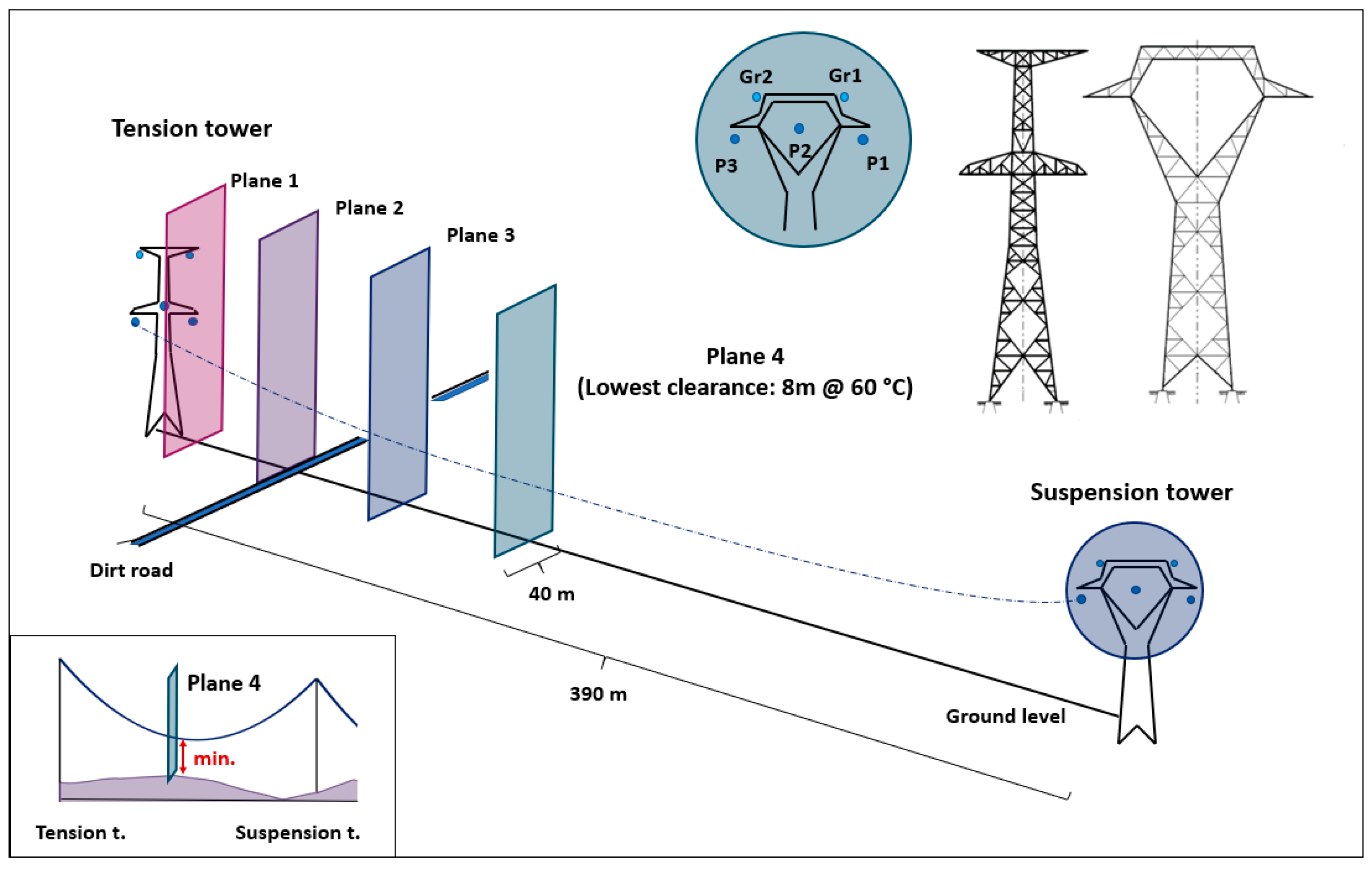
The chosen span is a section at one end of a tension span, meaning one boundary lattice tower is a suspension while the other is a tension one. The length of the span is 390 m, and according to the catenary curve and terrain profile analysis, the most critical sag point is 180 m from the tension tower.
Before starting the measurement, four measurement planes were defined, as illustrated in Figure 1.
Out of the four measuring planes, three play a prominent role. Measuring plane 1 extends directly below the tension tower’s insulator suspension points, the height of which above ground is nearly constant. There is a dirt road in the 2nd measurement plane, which should be treated as a critical case for pedestrian and agricultural vehicles. Measurement plane 4 is the plane containing the transmission line’s points with the smallest clearance (180 m from the tension tower) at the maximum design operating temperature of 60 °C. Measuring plane 3 was placed at equal distances from planes 2 and 4.
2.4. Data of the Line Monitoring Sensor
The applied sensor is an OTLM (Overhead Transmission Line Monitoring) manufactured superior line monitoring device, which measures the temperature, sag changes, and current load of the wire in real-time [29]. There is also a built-in camera that can also detect the ice layer deposited on the wire. The sensor has more than 20 different IEC (International Electrotechnical Commission) and MIL (Military) standards. The device is powered by a built-in AC adapter that starts operating at a minimum current of 65 A. During the on-the-spot measurements, its most important feature is the conductor temperature measuring, which has a ±2 °C deviation in the range from −40 °C to 125 °C. The conductor temperature resolution is 0.5 °C.
2.5. Results of the Field Measurement and Numerical Simulation
Five measurements were performed in the observed span (M1–M5). The first three were carried out in the first three measurement planes, one in each.
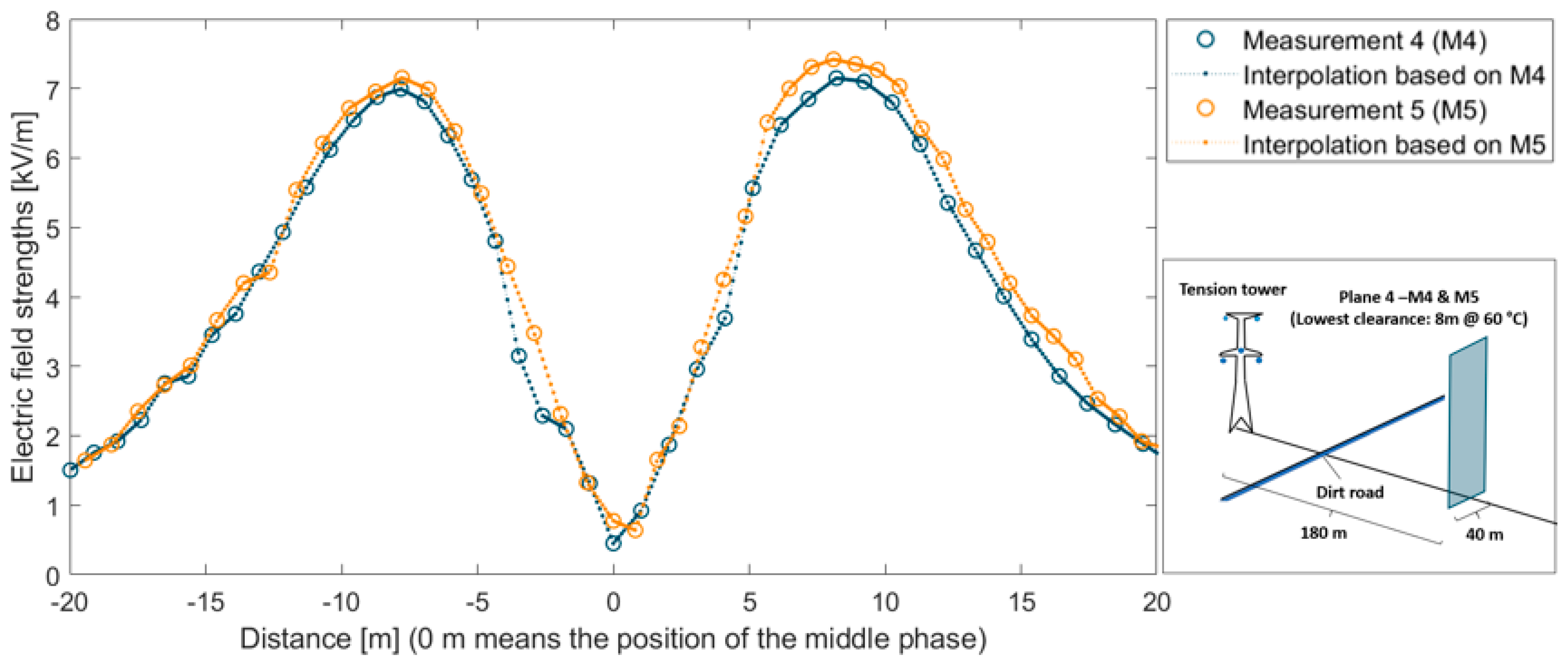
The results of measurement 4 and 5 (M4–M5) can be seen in Figure 2. Both were performed in measuring plane 4 because this plane includes the critical part of the OHL with the lowest clearance reserve. Figure 2 shows that the low-frequency electric field exceeds the 5 kV/m limit value required for the general public, while the temperature is well below the maximum operating limit.
Table 2 summarizes the results of the electric field measurements.
To validate the field measurements’ result, numerical, finite-element simulations were carried out for the observed OHL geometry.
The physics of the simulation is based on Equations (1)–(3):
where (J) is the current density in A/m2,
where (H) is the magnetic field strength in [A/m], (E) is the electric field strength in [V/m] and (D) is the electric displacement field in [As/m2].
where (E) is the electric field strength in [V/m] and (A) is the magnetic vector potential in [T/m].
In the analytical calculation, we used several approximations that do not affect the magnitude of the results, but greatly simplify the calculation. The conductors’ voltages were phase-shifted phase-to-ground voltages of a 400 kV system, and a grounded conductive plate modeled the surface of the ground at the bottom of the model. We assumed the conductors to be infinite in length parallel to the ground surface and one strand of aluminum. We considered the number of free charge carriers in the air to be 0. To increase the accuracy of the simulation, a finer meshing was set to the model. The physical parameters applied in the COMSOL model is in Table 3.
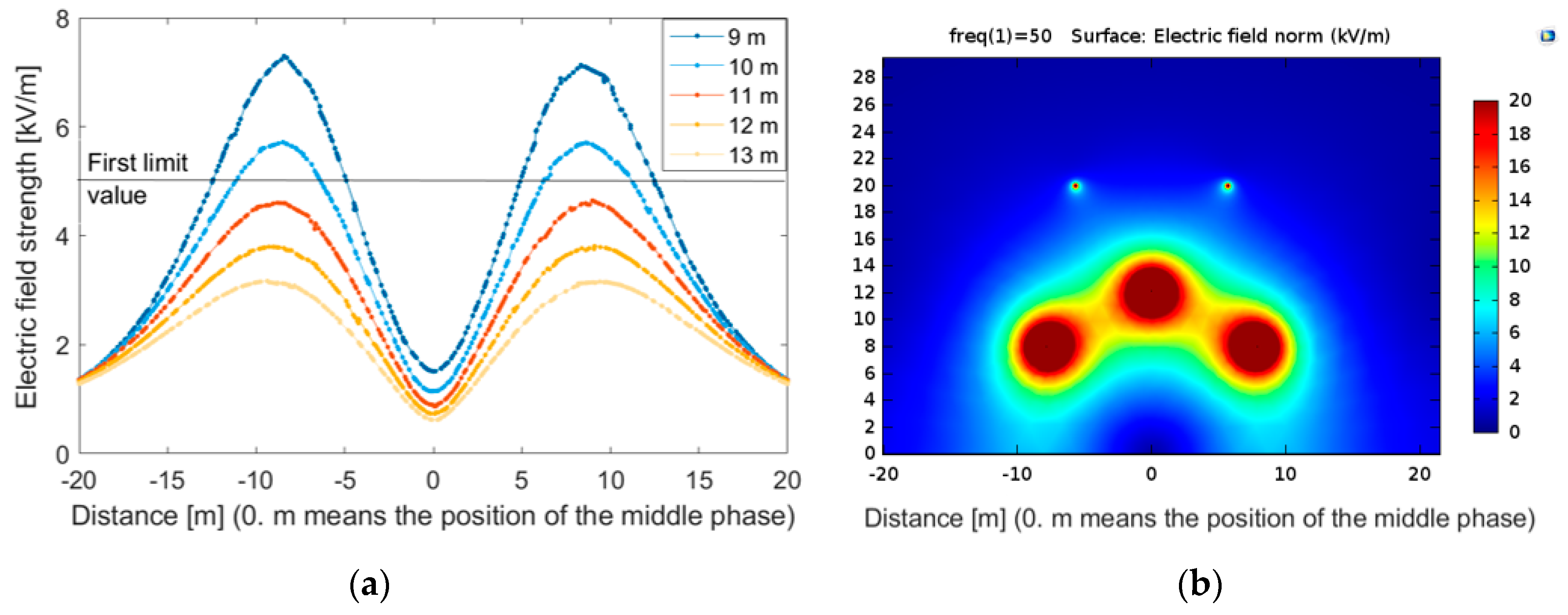
The results of the performed simulations are in Figure 3a,b.
Figure 3 presents the E-field distribution at different clearance values in the OHL’s cross-section at 1.8 m above the ground level. The curves represent cases with different clearance values from 13 m to 8 m, the legally defined safety distance for a 400 kV power line. Clearance values were simulated every 20 cm, but Figure 3a only includes whole meter results. Figure 3b shows visualization of the results for 8 m clearance around the power line.
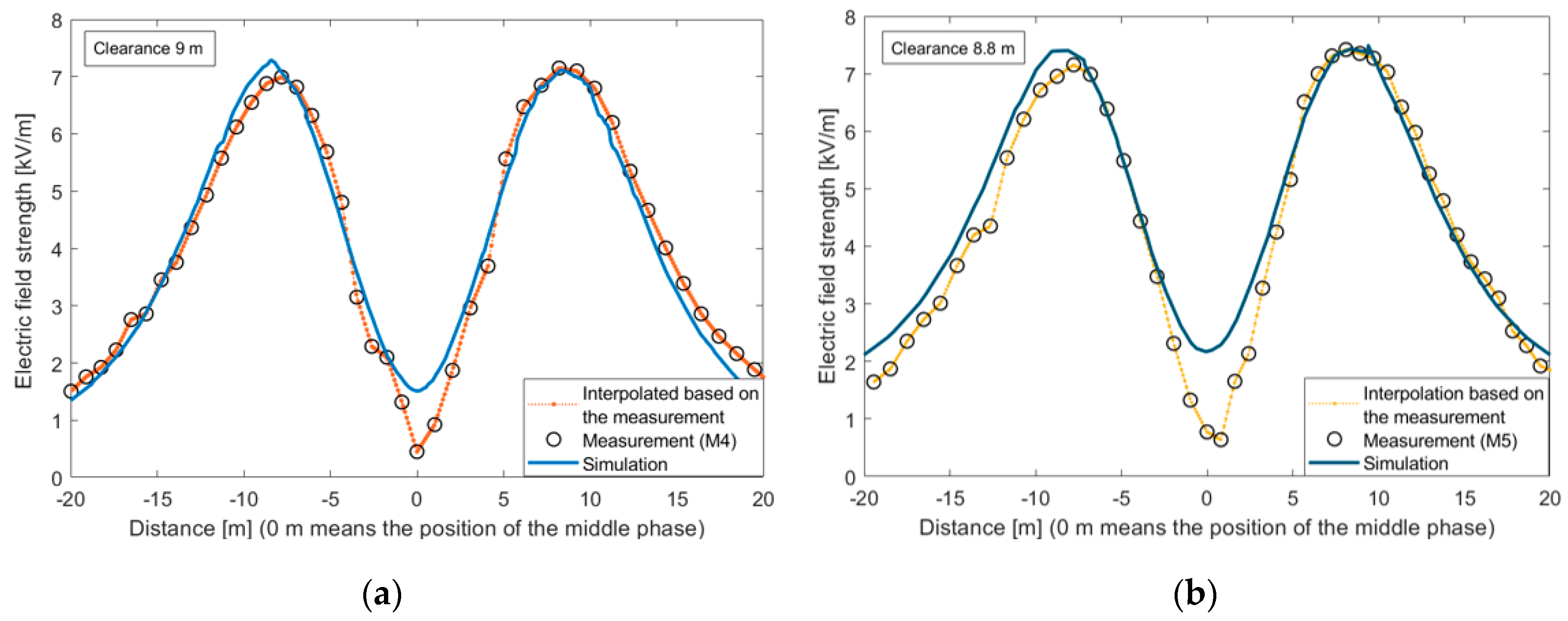
The line monitoring sensor measured the phase conductor temperature every 5 min, from which the clearance was determined mathematically [30,31]. The typical error rate of the clearance calculation algorithm is 0.1–0.15 m which was validated by the catenary curve and sensor measurements based on different methods in the FLEXITRANSTORE and FARCROSS projects. This way, the M4 and M5 measurements are compared to the simulation to validate the results (Figure 4).
For M4, the clearance was calculated to be 8.9 m. In Figure 4a, this is compared to the simulated curve at 9 m clearance. The curves’ general shape matches each other, such as the local peaks’ position and value. In COMSOL, we simulated the instantaneous values of the electric field formed with phase shifting of the voltages to illustrate the real field values around the line. The same situation is presented in Figure 4b; the only difference is that the calculated clearance was 8.7 m, and the curve was compared to the simulation at 8.8 m clearance.
According to the results, the field measurement and the numerical simulation are consistent with each other. The detailed comparison is provided in Table 4.
Based on Table 4, the field strength maximum values are the same with a good approximation. According to the simulation results, it is reasonable to say that the measurement results are a sound basis for further discussion.
2.6. Consequences from the Results
Based on the measurement and simulations, in the critical span, the electric field’s peak can be above 8 kV/m, which is 60% higher than the limit value for the general public. This phenomenon is unacceptable from the point of view of safety and security, as well as from a point of view of legal aspects.
Another critical question is how can these results be generalized for the whole length of the power line. For this purpose, the clearance values were calculated at the maximum operational temperature value of 60 °C in all the spans.
Table 5 describes the clearance and electric field peak values at 60 °C, which is the maximum allowed temperature of the conductor. According to the analysis, more than 65% of the spans are affected by the phenomenon. In the calculation, the phase conductor’s curve was described with a catenary curve represented in Equation (4) [30,31].
where σ is the horizontal component of the tensile stress and γ is weight force for a cross-section of 1 mm2 of a 1 m long conductor. For the sag calculation, Equation (5) served as a basis [30,31].
where (a) is the distance of the suspension points of the phase conductors.
Knowing the sag values at each distance, the clearance can be determined from the spread of the elevation profile and the conductor position. These results, however, do not consider that in some spans, the geometry may vary, and the error of the clearance simulation could be up to 15–20 cm. Although the limit values for safety distance and low-frequency electric field are clearly defined to ensure an adequate level of safety in the vicinity of the transmission lines individually, the specifications have not been harmonized in this case. There are clearly defined safety distance values at each voltage level in the standards applied for high voltage power lines, which does not guarantee compliance with the limit value for electric power fields. This situation needs to be avoided to comply with legal requirements that are in place.
The situation becomes more complicated if there is an endeavor to apply the DLR method. In these cases, the power line always operates near the maximum allowed conductor temperature increasing the operational risk. In this case, a more complex risk analysis should be applied taking into consideration the extension of the critical parts of the span in question, the co-occurrences of unfavorable weather and load parameters, and the accessibility of essential elements by humans.
3. Possible Solutions to Reduce the Electric Field
According to the legal requirement, it is necessary to reduce the electric field in the power lines’ vicinity. There are several options to accomplish this, but it is essential to consider the potential options makes more sense described below technical and economic aspects.
3.1. Material-Intensive Investments
Building new power lines is a strictly regulated and costly investment, and there is also a significant social resistance [32,33]. Alternatively, replacing towers or reconductoring of existing lines could lead to reduced electric field peak values, but retrofitting can take a long time [34]. Strengthening the existing power lines by replacing towers increases the clearance in all the spans; however, it is not economical for hundreds of kilometers of OHL. With retrofitting the primary aim is to reduce the sag, and increase the ground clearance. So-called HTLS (high-temperature low sag) conductors provide a possible solution for these cases since their long-term thermal load capacity is in the range of 200–220 °C, while their sag does not increase. This way, the same power can be transmitted with higher clearance values. The HTLS’s conductors operating experience is promising, but their widespread usage could significantly increase the investment cost. Reducing the upper thermal limit of the line and setting a new static line rating to the new temperature can also lead to result, but it is not economically advantageous. With this method the power transmitted through the line needs to be reduced significantly.
3.2. New Expert System Based on Dynamic Line Rating (DLR)
A new expert system based on DLR has been investigated to provide a technically and economically efficient solution for the electric field problem. With its application, the electric field can be ensured not to exceed its limit value, while the power line is fully utilized almost all the time. This system’s core is to determine what factor is responsible for the risk and decrease the maximum allowed conductor temperature to avoid electric field distribution problems. The method exploits the benefits of online monitoring in the real transfer capacity calculation. For real-time temperature tracking, a sensor needs to be installed onto the transmission line. The expert system provides a solution for the tension span equipped with the monitoring device, but it can be extended for the whole power line. The system’s operation is detailed below for a single tension span.
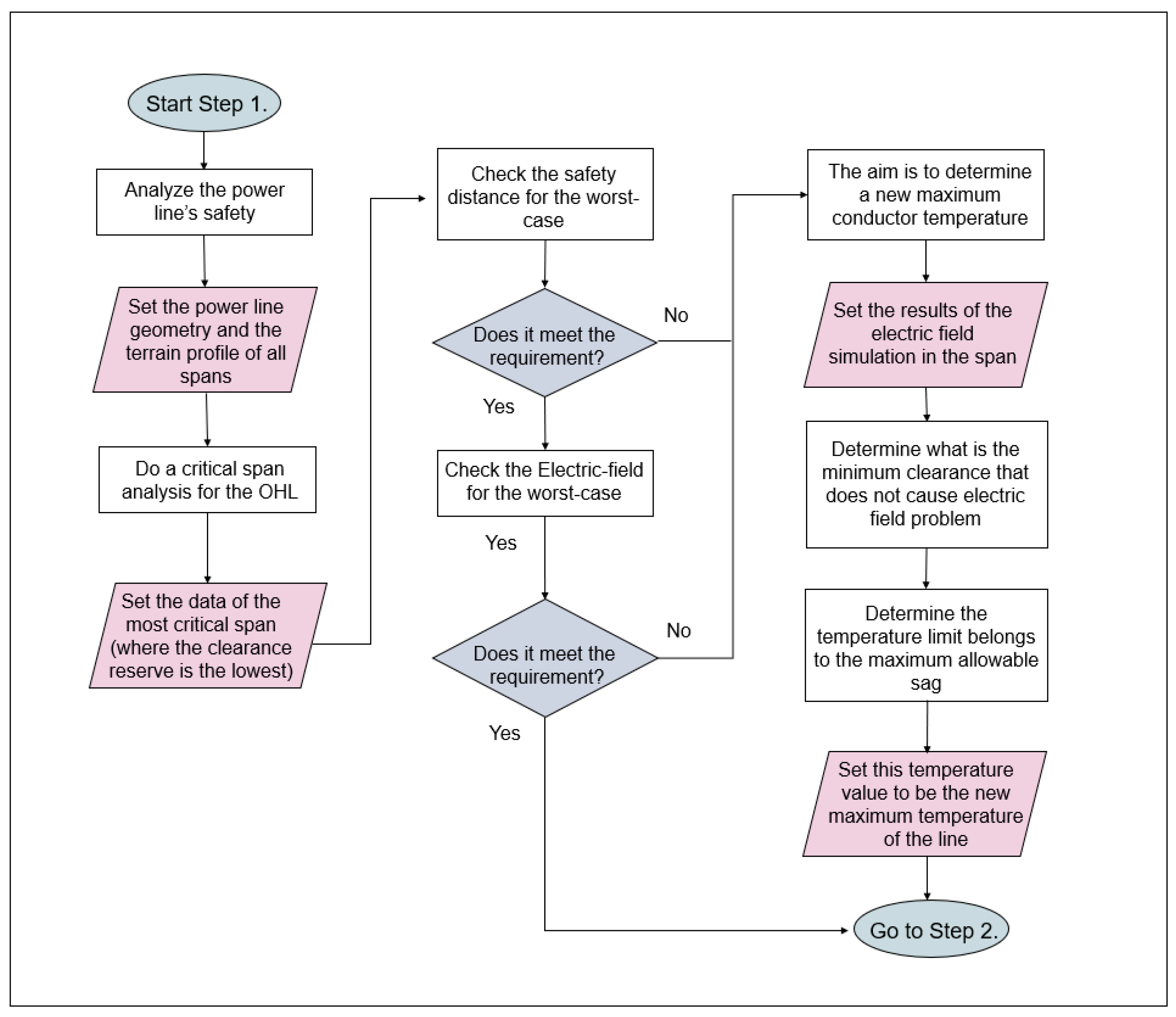
The operation of the expert system can be separated into two broad steps. The first one is a general analysis of the power line, while the second step concerns the observed tension span in which the sensor is installed. In Figure 5. The first step aims to find out whether the power line’s operation is at risk or not. First, a so-called critical span analysis needs to be performed. In this substep, all the tension spans are examined to find the lowest clearance value at the maximal operation conductor temperature. Via the analysis, the complete terrain profile needs to be considered, such as the objects and crossing elements under the power line. Once the critical span is determined, the safety distance needs to be checked at a worst-case conductor temperature. To get the clearance, first the phase conductor’s sag should be determined based on Equations (4) and (5). In some cases, the parabolic approximation of the conductors also gives a satisfactory result. If clearance meets the national regulation, the electric field’s peak value also needs to be checked. This step is necessary because not all the standards are harmonized, and as presented, the electric field can cause problems even if the safety distance is kept. If one of the two parameters does not meet the criterion, a new maximum wire temperature must be determined. In this substep, the numerical finite element simulation should be applied. Based on the simulation results, the sag value at which the electric field does not exceed the limit value can be selected. A conductor temperature can be assigned to the sag value, designated the new thermal limit for the regular operation condition.
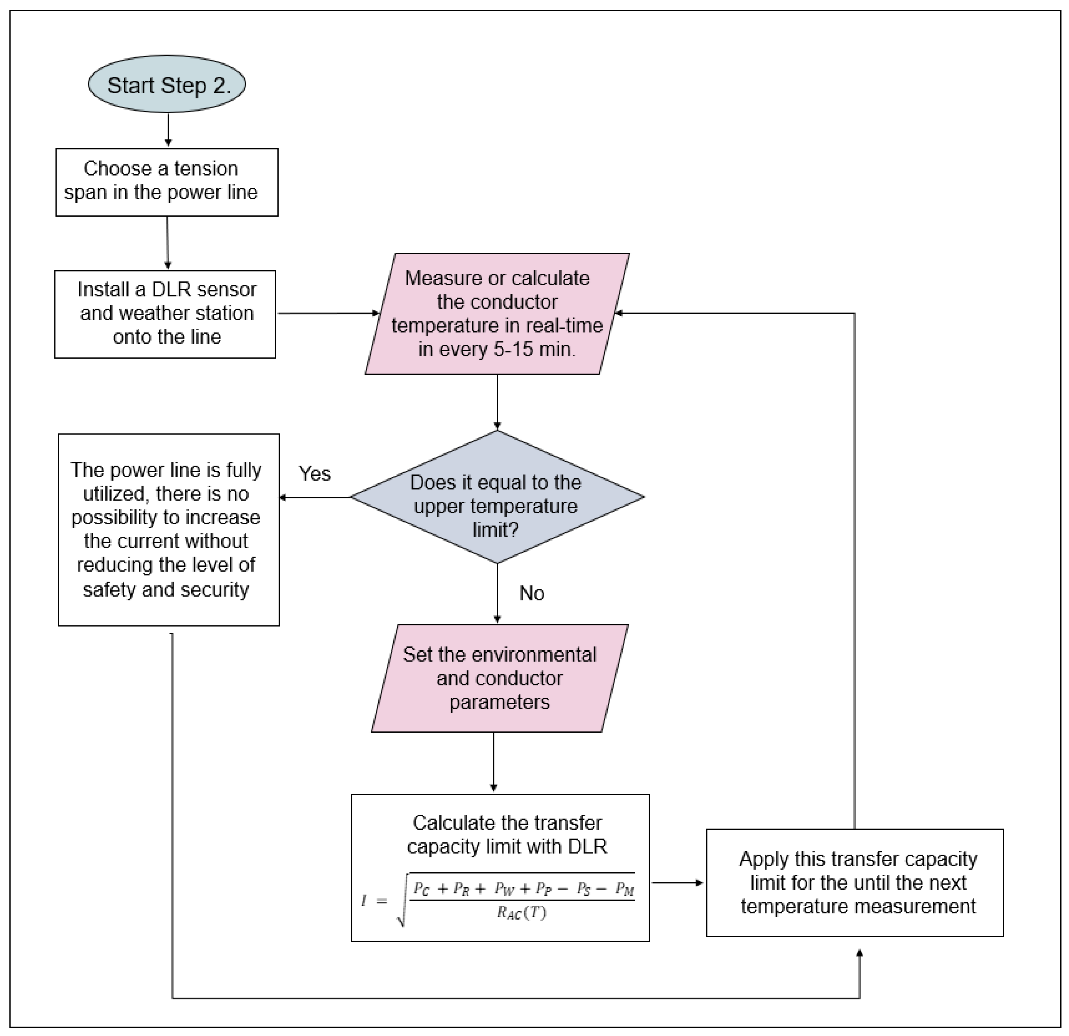
At the end of the first broad step, theoretically, there are two ways to increase the power line’s safety. One commonly used option is to apply SLR as a conventional line rating method. In the case of SLR, the new ampacity limit is the current calculated with the worst-case combination of the weather parameters. This results in a fixed transfer capacity value in the tension span for the whole year or season. For this reason, in all weather conditions other than the worst-case, the transmission line’s utilization will not be maximal, resulting in less transferable power for a large percentage of the time. That is why the second broad step based on DLR is necessary, so the expert system can ensure the line’s full utilization. The flowchart and the subtasks of the second step are shown in Figure 6.
To perform all the necessary substeps in the second step, a line monitoring sensor and weather stations need to be installed on the power line. The device must be able to measure the conductor temperature in real time every 5 to 15 min. It is favorable if the critical span is equipped with the line sensor to allow the expert system’s application to the whole line. When the conductor temperature is measured, a logical unit compares it to the maximum allowable conductor temperature, considering the operation state (such as the emergency case with emergency rating). If the temperatures are equal, there is no possibility to increase the transfer capacity without breaching the safety and security requirements. If the temperature is not close to the upper limit, the ampacity should be set as high as the thermal limit of the conductor.
This can be achieved by applying Equation (6) with all the necessary data measured from the weather stations [6].
where PJ is the Joule heating, PS the solar heating, PM the magnetic heating, PI the corona heating, PC the convective cooling, PR the radiative cooling, PW the evaporative cooling and PP the precipitation cooling. Transforming Equation (6) to Equation (7), the new current limit until the next sensor measurement is available [6].
where (I) means the ampacity limit, and the RAC is the temperature-dependent alternating current (AC) resistance of the conductor. Applying DLR can results in 20–30% surplus capacity contrarily to the SLR approach. In favorable cases, DLR’s surplus current can substitute for the ampacity loss from the reduced temperature. This way, it is possible to increase the line’s safety and security, meet the electric field legal requirements, and not cause economic loss. This algorithm is repeated continuously to ensure that the transfer capacity limit is always the theoretical maximum adjusted to whatever weather conditions allow. In summary, the significant benefits and strength of the new expert system are the following;
- the electric field’s peak is within the boundaries of the legal limits all the time;
- with DLR the full utilization of the line is ensured all the time;
- this method does not require high upgrade cost or other significant investment.
It is important to note that this expert system can be combined with other possible solutions mentioned before. Reconductoring the power line with HTLS conductors and applying the expert system on the line can result in higher ampacity limits, which can be vital from the transmission system operator point of view.
3.3. The Novelty of the Ampacity Calculation in the New, DLR-Based Expert System
The novelty of the new DLR-based expert system is twofold; on the one hand, it treats the electric field as a new input parameter, which was not previously discussed by any DLR calculation algorithm, and on the other hand, it further developed the international DLR models. Both the CIGRE (International Council on Large Electric Systems) and IEEE (Institute of Electrical and Electronics Engineers) DLR models are empirical formulas that discuss the external and internal factors influencing the conductor’s thermal state separately. None of these models previously calculated the cooling effect of precipitation, which, in addition to the average precipitation intensities in Europe (5–10 mm/h), can be expected to provide 5–8% additional load capacity compared to the basic physical models. The new expert system contains this cooling effect in Equations (6) and (7) to exploit the real ampacity limits of the OHLs [5,6,35].
Another innovation of the existing system is the way the conductor temperature is determined. In standard cases, the line monitoring sensor provides this parameter for the ampacity calculation; however, even if the device fails for any reason, an accurate, real-time conductor temperature is required. For this purpose, the BME (Budapest University of Technology and Economics) research group has developed a new neural network-based temperature calculation subsystem to ensure the conductor temperature parallel to the sensor measurements. This new subsystem’s accuracy is within the transmission line sensor’s measurement accuracy (±1.0 °C) based on simulations and international experience. In this way, the sensor temperature availability is ensured from several sides, which further increases the system’s reliability [5,9,35].
3.4. The Application of the Expert System for an Operating Power Line
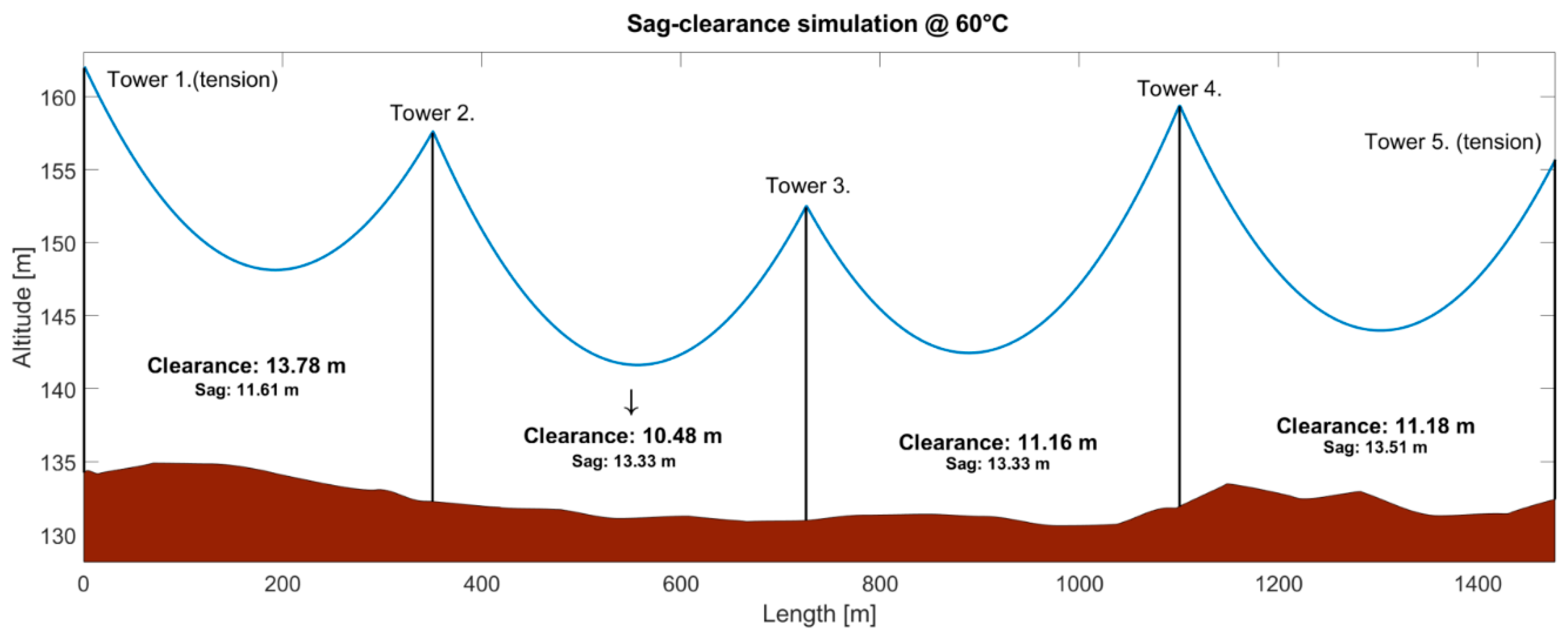
An example is given for one span of an active power line equipped with a DLR sensor to present the expert system’s applicability and its benefits in comparison to the static line rating. The OHL’s geometry and operating parameters are the same as detailed in Section 2 and Figure 1. According to the expert system, the critical span analysis was performed; the results are shown in Figure 7. The lowest clearance is 10.48 m in the span between towers 2 and 3, which should be equipped with a line monitoring sensor.
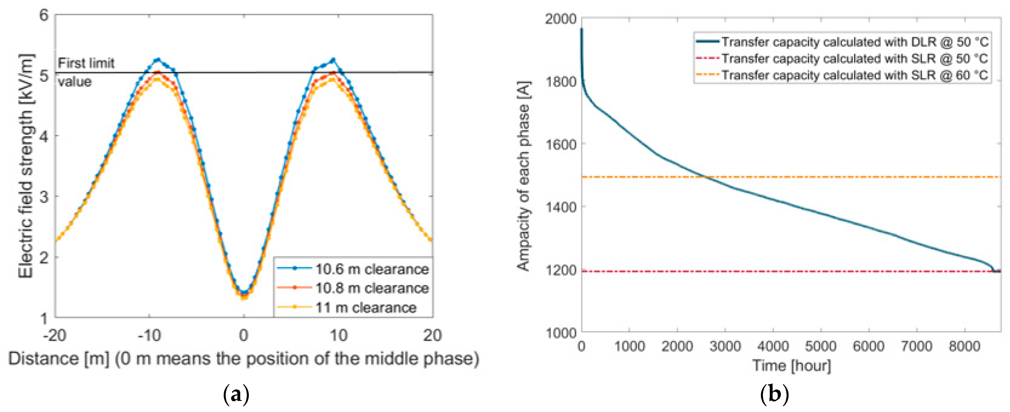
The span fulfills the necessary safety distance criterion of 8 m. The minimum clearance from the electric field’s peak value is determined to be 10.8 m from the finite-element simulation presented in Figure 8a.
Based on Figure 8a, the maximum operating temperature should be decreased from 60 °C to 50 °C, at which the lowest clearance is 10.84 m to fulfill the electric field criterion. The next step is to calculate the ampacity limit of the line. If the static line rating is applied—differing from the expert system—the worst-case parameters listed in Table 6 need to be used.
The new static line rating is 1193 ampere at each phase at 50 °C, which means 25.2% lower transferrable power than at 60 °C. With DLR in the expert system, this power loss can be prevented. Based on the sensor and weather stations’ real-time measurements, the ampacity is always at its theoretical maximum, which means a 20–30% average increase in power for a whole year. Figure 8b illustrates a so-called duration curve for a year that illustrates power lines’ capacity utilization. The area under the load duration curve is proportional to the amount of energy that can be transferred via OHLs, while the statistical curve itself represents what proportion of the year the given ampacity limit can be provided. According to Figure 8b, applying DLR with reduced maximum temperature can result in a higher ampacity limit to the non-reduced temperature case for more than 25% of the year. Thus, with the expert system’s help, it is possible to keep the electric field strength below the permissible limit, which increases safety and security and increases the ampacity limit of the transmission line for one year.
4. Conclusions
Dynamic line rating is a promising and cost-effective way of increasing the transfer capacity of the existing infrastructure. However, in the international literature it is not well established or well described how this method can directly affect high voltage lines’ safety. In this paper, we present examples of power lines in the vicinity of which the electric field distribution exceeds the general public’s limit value. This cannot be accepted from legal or safety points of view. To handle this phenomenon and ensure the level of safety, several methods are listed in the paper. To provide a cost-effective and efficient solution, a new expert system based on DLR has been analyzed. By applying this process, the safety level can increase to the acceptable level fulfilling the legal criteria. Via an example, it was shown that this expert system results in more economical results than the conventional static line rating with the line’s full utilization. In some cases, even higher ampacity can be reached than the transfer limit in the operating conditions at present. To sum up, this paper shows that dynamic line rating as a part of an expert system could directly benefit safety and security for the power lines, and has other advantageous attributes in addition to increased transfer capacity.
Author Contributions
Conceptualization, L.R. and B.N.; methodology, L.R. and B.N.; software, L.R.; formal analysis, L.R. and B.N.; investigation, L.R. and B.N.; resources, L.R. and B.N; data curation, L.R. and B.N.; writing—original draft preparation, L.R.; writing—review and editing, B.N.; visualization, L.R.; supervision, B.N.; project administration, B.N. All authors have read and agreed to the published version of the manuscript.
Funding
This research was funded by FARCROSS project of the European Union’s Horizon 2020 research and innovation programme under grant agreement No 864274.
Institutional Review Board Statement
Not applicable.
Informed Consent Statement
Not applicable.
Data Availability Statement
The data that support the findings of this study are available from the corresponding author, [LR], upon reasonable request.
Acknowledgments
This work has been developed in the High Voltage Laboratory of Budapest University of Technology and Economics within the boundaries of FARCROSS GA No 864274 project funded by Horizon2020. The project aims to connect major stakeholders of the energy value chain and demonstrate integrated hardware and software solutions that will facilitate the “unlocking” of the resources for the cross-border electricity flows and regional cooperation.
![Applsci 11 00492 i001]()

Conflicts of Interest
The authors declare no conflict of interest.
References
- McCall, J.C.; Servatius, B. Enhanced Economic and Operational Advantages of Next Generation Dynamic Line Rating Systems. In Proceedings of the 2016 CIGRE Grid of the Future Symposium, Philadelphia, PA, USA, 31 October 2016. [Google Scholar]
- Schiel, C.; Lind, P.G.; Maass, P. Resilience of electricity grids against transmission line overloads under wind power injection at different nodes. Sci. Rep. 2017, 7, 11562. [Google Scholar] [CrossRef] [PubMed] [Green Version]
- European Environment Agency. Renewable Energy in Europe—2018, Recent Growth and Knock-On Effects; Publications Office of the European Union: Luxembourg, 2018. [Google Scholar]
- Philips, A. Evaluation of Instrumentation and Dynamic Thermal Ratings for Overhead Lines, Final Report; Electric Power Research Institute/New York Power Authority: White Plains, NY, USA, 2013.
- Rácz, L.; Szabó, D.; Németh, B.; Göcsei, G. Grid Management Technology for the Integration of Renewable Energy Sources into the Transmission System. In Proceedings of the 7th International Conference on Renewable Energy Research and Applications, Paris, France, 14–17 October 2018. [Google Scholar]
- CIGRE 601, Working Group B2.43. Guide for Thermal Rating Calculations of Overhead Lines; CIGRE: Paris, France, 2014. [Google Scholar]
- Viola, T.; Németh, B.; Göcsei, G. Applicability of DLR Sensors in High Voltage Systems. In Proceedings of the 6th International Youth Conference on Energy, Budapest, Hungary, 21–24 June 2017; pp. 1–6. [Google Scholar] [CrossRef]
- Rácz, L.; Szabó, D.; Göcsei, G.; Németh, B. Application of Monte Carlo Methods in Probability—Based Dynamic Line Rating Models. In Technological Innovation for Industry and Service Systems, Proceedings of the Doctoral Conference on Computing, Electrical and Industrial Systems, Costa de Caparica, Portugal, 8–10 May 2019; Camarinha-Matos, L.M., Almeida, R., Oliveira, J., Eds.; Springer: Berlin/Heidelberg, Germany, 2019; pp. 11–124. [Google Scholar]
- Rácz, L.; Németh, B. Investigation of dynamic electricity line rating based on neural networks. Energetika 2018, 64, 74–83. [Google Scholar] [CrossRef]
- International Commission on Non-Ionizing Radiation Protection. Guidelines for Limiting Exposure To Time-Varying Electric And Magnetic Fields (1 Hz–100 kHz). Health Phys. 2010, 99, 818–836. [Google Scholar]
- World Health Organization; International Agency for Research on Cancer. Non-Ionizing Radiation, Part 1: Static and Extremely Low-Frequency (ELF) Electric and Magnetic Fields. In IARC Monographs on the Evaluation of Carcinogenic Risks to Humans; IARCPress: Lyon, France, 2002; Volume 80. [Google Scholar]
- Deltuva, R.; Lukočius, R. Distribution of Magnetic Field in 400 kV Double-Circuit Transmission Lines. Appl. Sci. 2020, 10, 3266. [Google Scholar] [CrossRef]
- Frigura-Iliasa, M.; Baloi, F.I.; Frigura-Iliasa, F.M.; Simo, A.; Musuroi, S.; Andea, P. Health-Related Electromagnetic Field Assessment in the Proximity of High Voltage Power Equipment. Appl. Sci. 2020, 10, 260. [Google Scholar] [CrossRef] [Green Version]
- Gajšek, P.; Ravazzani, P.; Grellier, J.; Samaras, T.; Bakos, J.; Thuróczy, G. Review of Studies Concerning Electromagnetic Field (EMF) Exposure Assessment in Europe: Low Frequency Fields (50 Hz–100 kHz). Int. J. Environ. Res. Public Health 2016, 13, 875. [Google Scholar] [CrossRef] [PubMed] [Green Version]
- Reilly, J. Applied Bioelectricity: From Electrical Stimulation to Electropathology; Springer: New York, NY, USA, 1998. [Google Scholar]
- World Health Organization. Environmental Health Criteria 238 Extremely Low Frequency (ELF) Fields; WHO: Geneva, Switzerland, 2007. [Google Scholar]
- Xi, W.; Stuchly, M. High spatial resolution analysis of electric currents induced in men by ELF magnetic fields. Appl. Comput. Electromagn. Soc. 1994, 9, 127–134. [Google Scholar]
- Trlep, M.; Hamler, A.; Jesenik, M.; Stumberger, B. Electric Field Distribution Under Transmission Lines Dependent on Ground Surface. IEEE Trans. Magn. 2009, 45, 1748–1751. [Google Scholar] [CrossRef]
- Florkowska, B.; Jackowicz-Korczynski, A.; Timler, M. Analysis of electric field distribution around the high-voltage overhead transmission lines with an ADSS fiber-optic cable. IEEE Trans. Power Deliv. 2004, 19, 1183–1189. [Google Scholar] [CrossRef]
- Kumru, C.F.; Kocatepe, C.; Arikan, O. An Investigation on Electric Field Distribution around 380 kV Transmission Line for Various Pylon Models, World Academy of Science. Int. J. Electr. Comput. Eng. Electr. Commun. Eng. 2015, 9, 888–891. [Google Scholar]
- Ruiz, J.-R.R.; Espinosa, A.G.; Morera, X.A. Electric Field Effects of Bundle and Stranded Conductors in Overhead Power Lines. Comput. Appl. Eng. Educ. 2011, 19, 107–114. [Google Scholar] [CrossRef]
- Tanaka, K.; Mizuno, Y.; Naito, K. Measurement of Power Frequency Electric and Magnetic Fields Near Power Facilities in Several Countries. IEEE Trans. Power Deliv. 2011, 26, 1508–1513. [Google Scholar] [CrossRef]
- Frigura-Iliasa, M.; Baloi, F.I.; Olariu, A.F.; Petrenci, R.C. Magnetic Field Assessment in the Proximity of High Voltage Power Station Equipment. In Proceedings of the 2019 20th International Scientific Conference on Electric Power Engineering, Kouty nad Desnou, Czech Republic, 15–17 May 2019; pp. 1–4. [Google Scholar] [CrossRef]
- Göcsei, G.; Németh, B.; Tarcsa, D. Extra low frequency electric and magnetic fields during live-line maintenance. In Proceedings of the 2013 IEEE Electrical Insulation Conference, Ottawa, ON, Canada, 2–5 June 2013; pp. 100–104. [Google Scholar] [CrossRef]
- Flexitranstore. Available online: http://www.flexitranstore.eu/ (accessed on 18 November 2020).
- Farcross. Available online: https://farcross.eu/ (accessed on 18 November 2020).
- CIGRE, Working Group C4.203. Technical Guide for Measurement of Low Frequency Electric and Magnetic Fields Near Overhead Power Lines; CIGRE: Paris, France, 2009. [Google Scholar]
- Rácz, L.; Szabó, D.; Göcsei, G. Investigation of Electric and Magnetic Field in the Application of Dynamic Line Rating. In Lecture Notes in Electrical Engineering, Proceedings of the 21st International Symposium on High Voltage Engineering, Budapest, Hungary, 26–30 August 2020; Springer: Berlin/Heidelberg, Germany, 2020; pp. 145–153. [Google Scholar]
- OTLM. Available online: https://www.otlm.eu/ (accessed on 26 December 2020).
- Perneczky, G. Szabadvezetékek Feszítése (Tension in the Overhead Lines); Műszaki Könyvkiadó: Budapest, Hungary, 1968. [Google Scholar]
- Bayliss, C.; Hardy, B. Transmission and Distribution Electrical Engineering, 4th ed.; Elsevier: Oxford, UK, 2012. [Google Scholar]
- Andrade, J.; Baldick, R. Estimation of Transmission Costs for New Generation, White Paper UTEI/2016-09-1. 2016. Available online: http://energy.utexas.edu/the-full-cost-of-electricity-fce/ (accessed on 18 November 2020).
- European Commission. Guidance on Energy Transmission Infrastructure and EU Nature Legislation; European Commission: Brussels, Belgium, 2018. [Google Scholar]
- Nuchprayoon, S.; Chaichana, A. Cost Evaluation of Current Uprating of Overhead Transmission Lines Using ACSR and HTLS Conductors. In Proceedings of the 2017 IEEE International Conference on Environment and Electrical Engineering and 2017 IEEE Industrial and Commercial Power Systems Europe, Milan, Italy, 6–9 June 2017; pp. 1–5. [Google Scholar] [CrossRef]
- Németh, B.; Göcsei, G.; Rácz, L.; Szabó, D. Development and Realization of a Complex Transmission Line Management System. Presented at the 2020 CIGRE Paris Session—PS2 Enhancing Overhead Line Performance [Online], Paris, France, 24 August 2020. Available online: https://e-cigre.org/publication/session2020-2020-cigre-session (accessed on 26 December 2020).
Figure 1.
Measuring positions in the selected span.

Figure 2.
Measured electric field distribution at 1.8 m height above the ground (M4–M5).

Figure 3.
Simulated electric field distribution at 1.8 m height above the ground. (a) Results at phase conductor clearance from 9 m to 13 m; (b) results at phase conductor clearance of 8 m.
Figure 3.
Simulated electric field distribution at 1.8 m height above the ground. (a) Results at phase conductor clearance from 9 m to 13 m; (b) results at phase conductor clearance of 8 m.

Figure 4.
Comparing simulated and measured electric field distribution. (a) M4 measurement curve and E-field simulation at clearance 9 m; (b) M5 measurement curve and E-field simulation at clearance 8.8 m.
Figure 4.
Comparing simulated and measured electric field distribution. (a) M4 measurement curve and E-field simulation at clearance 9 m; (b) M5 measurement curve and E-field simulation at clearance 8.8 m.

Figure 5.
Process drawing of the first step of the new dynamic line rating (DLR)-based expert system.
Figure 5.
Process drawing of the first step of the new dynamic line rating (DLR)-based expert system.

Figure 6.
Process drawing of the second step of the new DLR-based expert system.

Figure 7.
The critical span from the aspect of clearance, equipped with DLR sensor.

Figure 8.
Results of the expert system. (a) Simulated electric field values in the critical span at different clearances; (b) transfer capacity 1-year duration curve calculated with DLR compared to ampacity calculated with SLR.
Figure 8.
Results of the expert system. (a) Simulated electric field values in the critical span at different clearances; (b) transfer capacity 1-year duration curve calculated with DLR compared to ampacity calculated with SLR.


Table 1.
Reference levels for the general public and occupational exposure to the time-varying electric field and magnetic flux density [10].
Table 1.
Reference levels for the general public and occupational exposure to the time-varying electric field and magnetic flux density [10].
| Exposure | Frequency Range | Electric Field | Magnetic Flux Density |
|---|---|---|---|
| General public | 50 Hz | 5 [kV/m] | 200 [µT] |
| Occupational | 50 Hz | 10 [kV/m] | 1000 [µT] |
Table 2.
Results of the electric field measurement.
| Measuring Plane | Load of the OHL (Overhead Line) | Ambient Temperature | Max. Value of the E-Field |
|---|---|---|---|
| Plane 1 | 276.5 A | 34.5 °C | 1.277 kV/m |
| Plane 2 | 292.0 A | 35.0 °C | 3.060 kV/m |
| Plane 3 | 348.0 A | 36.0 °C | 4.679 kV/m |
| Plane 4 | 278.5 A | 33.8 °C | 7.150 kV/m |
| Plane 4 | 348.0 A | 35.5 °C | 7.420 kV/m |
Table 3.
Conductor and insulator model parameters.
| Description | Value | Unit |
|---|---|---|
| Aluminum diameter | 31.06 | [mm] |
| Aluminum conductivity | 37.74 | [MS/m] |
| Relative permittivity of Aluminum | 1 | [-] |
| Relative permittivity of air | 1 | [-] |
Table 4.
Comparison of the measurement and the simulation.
| Case | Clearance | Peak Value | Position of the Peak |
|---|---|---|---|
| M4 | 8.9 m | 7.150 kV/m | 8.20 m |
| S4 | 9.00 m | 7.276 kV/m | −8.57 m |
| Relative error | 1.1% | −0.02% | 0.04 % |
| M5 | 8.7 m | 7.420 kV/m | 8.10 m |
| S5 | 8.80 m | 7.400 kV/m | −8.06 m |
| Relative error | 1.1% | −0.01% | 0.01 % |
Table 5.
Extension of the results to the whole power line at 60 °C.
| Safety Margin | Number | Electric Field Peak |
|---|---|---|
| 8–9 m safety margin | 26 | 7.07–8.22 kV/m |
| 9–10 m safety margin | 21 | 6.25–7.07 kV/m |
| 10–11 m safety margin | 24 | 5.61–6.25 kV/m |
| 11–12 m safety margin | 15 | 5.10–5.61 kV/m |
| 12–12.2 m safety margin | 5 | 5.00–5.10 kV/m |
| Safety margin less than 12.2 m | 91 | Above 5.00 kV/m |
| Safety margin more than 12.2 m | 48 | Below 5.00 kV/m |
Table 6.
Weather parameters for static line rating 1.
| Symbol | Weather Parameter | Value | Measuring Unit |
|---|---|---|---|
| Ta | Ambient temperature | 30 | [°C] |
| ws | Wind speed | 0.61 | [m/s] |
| wd | Wind direction | 90 | [°] |
| S | Solar radiation | 900 | [W/m2] |
| P | Precipitation | 0 | [mm/h] |
| ε | Emissivity factor | 0.6 | [-] |
1 These values can vary from territories depending on the prevailing climate.
Publisher’s Note: MDPI stays neutral with regard to jurisdictional claims in published maps and institutional affiliations. |
© 2021 by the authors. Licensee MDPI, Basel, Switzerland. This article is an open access article distributed under the terms and conditions of the Creative Commons Attribution (CC BY) license (http://creativecommons.org/licenses/by/4.0/).
Share and Cite
MDPI and ACS Style
Rácz, L.; Németh, B. Dynamic Line Rating—An Effective Method to Increase the Safety of Power Lines. Appl. Sci. 2021, 11, 492. https://0-doi-org.brum.beds.ac.uk/10.3390/app11020492
AMA Style
Rácz L, Németh B. Dynamic Line Rating—An Effective Method to Increase the Safety of Power Lines. Applied Sciences. 2021; 11(2):492. https://0-doi-org.brum.beds.ac.uk/10.3390/app11020492
Chicago/Turabian StyleRácz, Levente, and Bálint Németh. 2021. "Dynamic Line Rating—An Effective Method to Increase the Safety of Power Lines" Applied Sciences 11, no. 2: 492. https://0-doi-org.brum.beds.ac.uk/10.3390/app11020492
Note that from the first issue of 2016, this journal uses article numbers instead of page numbers. See further details here.