
Kinematic In Situ Self-Calibration of a Backpack-Based Multi-Beam LiDAR System


1
Department of Civil and Environmental Engineering, Myongji University, 116 Myongji-ro, Cheoin-gu, Yongin 17058, Gyeonggi-do, Korea
2
Department of Civil & Environmental Engineering, Seoul National University, 599 Gwanak-ro 1, Gwanak-gu, Seoul 08826, Korea
3
Lyles School of Civil Engineering, Purdue University, 610 Purdue Mall, West Lafayette, IN 47907, USA
*
Author to whom correspondence should be addressed.
Appl. Sci. 2021, 11(3), 945; https://0-doi-org.brum.beds.ac.uk/10.3390/app11030945
Submission received: 27 November 2020
/
Revised: 8 January 2021
/
Accepted: 19 January 2021
/
Published: 21 January 2021
(This article belongs to the Special Issue Image Simulation in Remote Sensing)
Abstract
:Light Detection and Ranging (LiDAR) remote sensing technology provides a more efficient means to acquire accurate 3D information from large-scale environments. Among the variety of LiDAR sensors, Multi-Beam LiDAR (MBL) sensors are one of the most extensively applied scanner types for mobile applications. Despite the efficiency of these sensors, their observation accuracy is relatively low for effective use in mobile mapping applications, which require measurements at a higher level of accuracy. In addition, measurement instability of MBL demonstrates that frequent re-calibration is necessary to maintain a high level of accuracy. Therefore, frequent in situ calibration prior to data acquisition is an essential step in order to meet the accuracy-level requirements and to implement these scanners for precise mobile applications. In this study, kinematic in situ self-calibration of a backpack-based MBL system was investigated to develop an accurate backpack-based mobile mapping system. First, simulated datasets were generated for the experiments and tested in a controlled environment to inspect the minimum network configuration for self-calibration. For this purpose, our own-developed simulator program was first utilized to generate simulation datasets with various observation settings, network configurations, test sites, and targets. Afterwards, self-calibration was carried out using the simulation datasets. Second, real datasets were captured in a kinematic situation so as to compare the calibration results with the simulation experiments. The results demonstrate that the kinematic self-calibration of the backpack-based MBL system could improve the point cloud accuracy with Root Mean Square Error (RMSE) of planar misclosure up to 81%. Conclusively, in situ self-calibration of the backpack-based MBL system can be performed using on-site datasets, reaching the higher accuracy of point cloud. In addition, this method, by performing automatic calibration using the scan data, has the potential to be adapted to on-line re-calibration.
1. Introduction
Over the past few years, significant developments of laser scanning technology have increased the feasibility of acquiring large amounts of accurate geometric 3D data. The demand for 3D observation has increased as well with the development of automatic digital image analysis, namely artificial intelligence. In this context, laser scanners have become a fundamental means to acquire 3D information in a manner that is effective enough to satisfy the growing demand in this field [1]. This trend is particularly relevant in civil engineering, robotics, and computer vision, due to those fields’ high usage of laser scanners as routine measurement techniques for applications such as 3D modeling and mapping [2,3], efficient building management [4,5], and the transformation of structural health monitoring [6,7]. Extending the application of laser scanners from geomatics to these domains has resulted in the emergence of new areas for potential implementation, which requires the development of more efficient and accurate acquisition systems [8]. More recently, Light Detection and Ranging (LiDAR) sensors have become more portable, compact, and readily available to be extended to mobile applications. The advancement of modern technology has expanded the use of LiDAR sensors to a variety of applications including mobile mapping, surveying, and autonomous vehicles. In particular, Multi-Beam LiDAR (MBL) is one of the most extensively used and favored sensors for mobile applications, because the sensors are relatively lightweight, compact, and cheap. MBL, manufactured by Velodyne LiDAR, has been widely used both in research and the industrial field [9,10,11,12,13,14,15,16,17]. Particularly, backpack-based 3D mapping using Velodyne LiDAR has been a popular mobile application. Leica Pegasus [18], Viametris bMS3D [19], GreenValley LiBackpack [20], and Gexcel Heron [21] are examples of the commercial backpack-based mobile mapping system. These solutions use two Velodyne VLP-16 units to perform odometry for georeferencing and 3D mobile mapping including Simultaneous Localization and Mapping (SLAM). Along with the growing need for 3D information, these commercial backpack-based mapping systems were released to match the demand for quick data acquisition and fieldwork planning; however, there are drawbacks that require further improvement in terms of accuracy and cost [22]. In this context, developing an accurate and affordable backpack-based mapping system is still an interest in this field.
For successful and effective mobile LiDAR scanning, two fundamental issues need to be addressed: georeferencing and sensor calibration. Georeferencing is the conversion of a local coordinate system to one global coordinate system combining all point clouds into the same coordinate system. Sensor calibration removes systematic errors inherent to sensors and can accomplish quality assurance to maximize the accuracy of observation. These two key processes are not independent, which means that the more accurate the sensor system that is built, the more accurate georeferencing becomes, so that the overall accuracy of surveying can be improved. Therefore, establishing an accurate mobile LiDAR sensor system is the most significant step. Even though MBL provides a cost-efficient and portable option, their observation accuracy is lower than conventional Terrestrial Laser Scanners (TLS) in general. They include systematic errors, which can affect the overall accuracy of the scanned data. Since each mechanically designed laser measures the range by time-of-flight system and encoder angle, the point cloud inevitably contains systematic errors in range and angle measurements with respect to each laser. These systematic errors can cause translations and rotations in the point cloud data. As a result, for precise mobile mapping and surveying, the overall accuracy of the point cloud data needs to be improved [23].
LiDAR self-calibration can remove the systematic errors inherent in the sensor and thus improve the overall accuracy of point cloud by reducing the Root Mean Square Error (RMSE) associated with registration and check points [24]. It also can reduce the need for point cloud outlier removal as a post-processing step. In the case of MBL, various studies in the literature have performed self-calibration using modified manufacturer-based calibration parameters. They also have confirmed the potential of applying these sensors as a basis for obtaining a highly accurate mobile mapping platform. A calibration of Velodyne HDL-64E, which is Velodyne’s first generation of MBL consisting of 64 laser channels, can be found in the literature. Static calibration of Velodyne HDL-64E using plane-based targets achieved a 3D RMSE up to 0.013 m [25], while optimization-based calibration showed standard deviations of planar data from 0.006 to 0.037 m [26]. Moreover, minimizing the discrepancies between the point cloud and pattern planes attained 0.0156 m of point cloud accuracy [27]. In addition to the installed target-based approaches, the static on-site re-calibration approach using planes accomplished 0.013 m of planar misclosure [28]. Besides, the kinematic calibration of HDL-64E on a moving vehicle attained 0.023 m of planar RMS residuals [29]. Velodyne HDL-32E mounted on a vehicle, which consists of 32 laser channels, was also calibrated using cylinder-based self-calibration and improved the accuracy level to 0.008 m in static mode and 0.014 m in kinematic mode [30]. The calibration of the most recent generation of MBL by Velodyne, VLP-16, showed 0.025 m of planar RMSE residuals [31]. However, the system parameters may still be inconsistent, even after self-calibration, due to the instability inherent in the scanning system. Temporal stability analysis of an MBL demonstrated that the measurement stability is slightly higher than the quantization level, which stresses the need for periodic re-calibration of the LiDAR sensor to maintain a high level of accuracy [32]. Since measurement stability analysis showed inconsistency in range observation, there is a chance that the calibration parameters might change during data acquisition. As a result, periodic in situ calibration should be performed to increase and maintain the heightened overall accuracy of the point cloud for a backpack-based MBL system. This leads to our objective of the study, which is the kinematic self-calibration method that can be performed continually during the data acquisition.
In this respect, this study aimed to perform kinematic in situ self-calibration of a backpack-based MBL system for the purposes of easy, efficient and frequent periodical self-calibration prior to data acquisition. First, self-calibration was conducted with simulation datasets to examine the minimum network configuration for the in situ self-calibration of backpack-based MBL system. Second, based on the analysis from the simulation experiments, reals datasets were acquired using our own backpack system. The accuracy of the results was analyzed by investigating planar misclosure after the adjustment, the correlations between parameters, measurement residuals, and the standard deviation of the estimated parameters. The remainder of this study is organized as follows. Section 2 presents the configuration and specifications of the sensor system used in this study. Section 3 covers the mathematical models, which are an observation model, a systematic error model, a functional model, and a least squares solution for the adjustment. Section 4 outlines the experimental set-ups and the calibration datasets for the investigation of the minimum network configuration and observation requirements. It also includes the results of the experiments and accuracy analysis. Section 5 provides a discussion of the proposed method in terms of accuracy and benefits. In conclusion, Section 6 summarizes the findings of the study along with possible future work.
2. Backpack-Based Sensor System
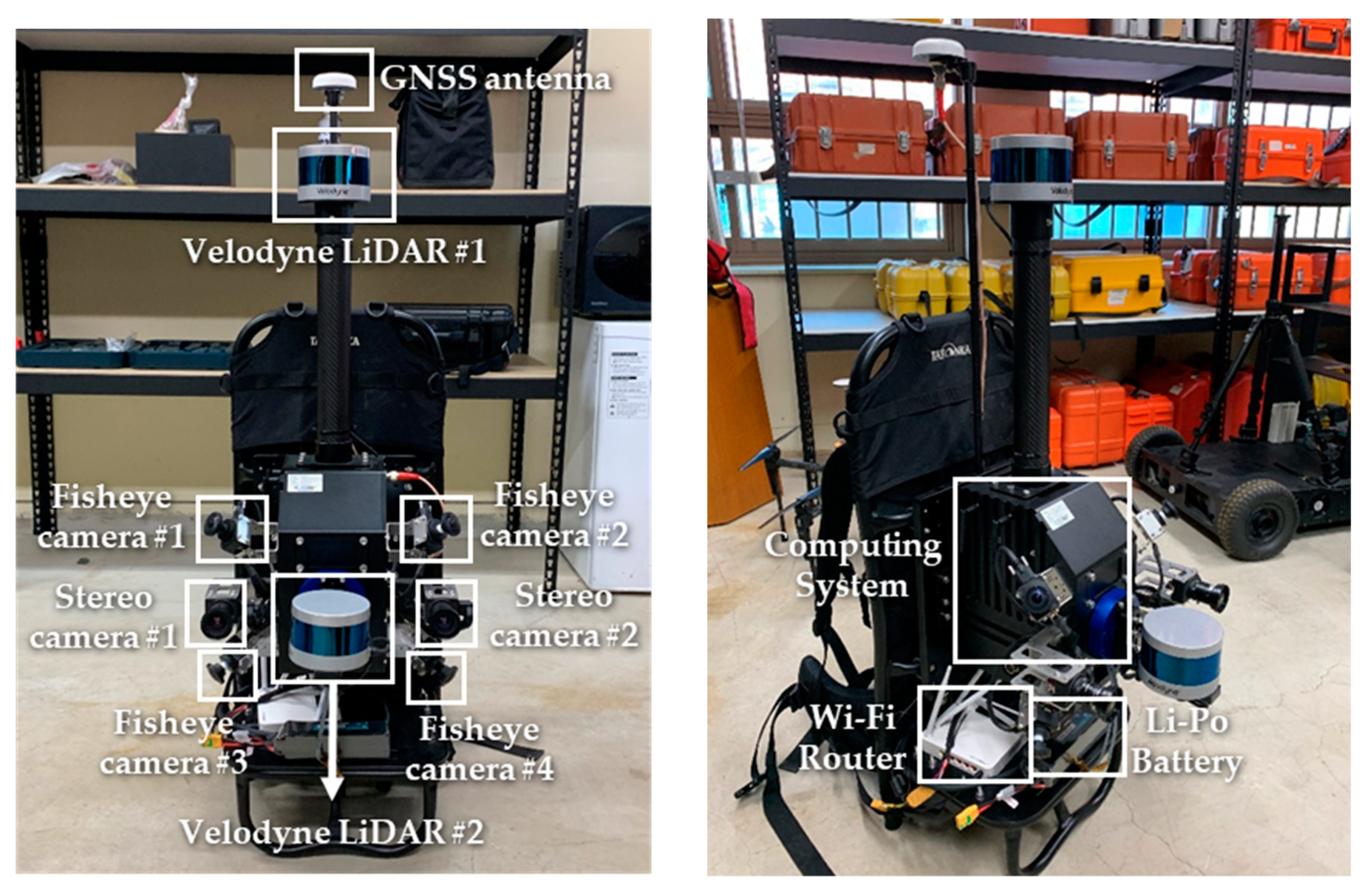
The backpack-based MBL system used in this study consists of two LiDAR sensors, six optical cameras, and a Global Navigation Satellite System (GNSS)/Inertial Navigation System (INS) (Figure 1). The configuration of the involved sensors was determined to have minimum occlusion and maximum Field of View (FOV). The sensors are all integrated into a core computing system, which receives all sensor data and synchronizes into Universal Time Coordinated (UTC) timestamps. The Inertial Measurement Unit (IMU) was not described in Figure 1 since the unit is embedded in the computing system.
2.1. LiDAR Sensors
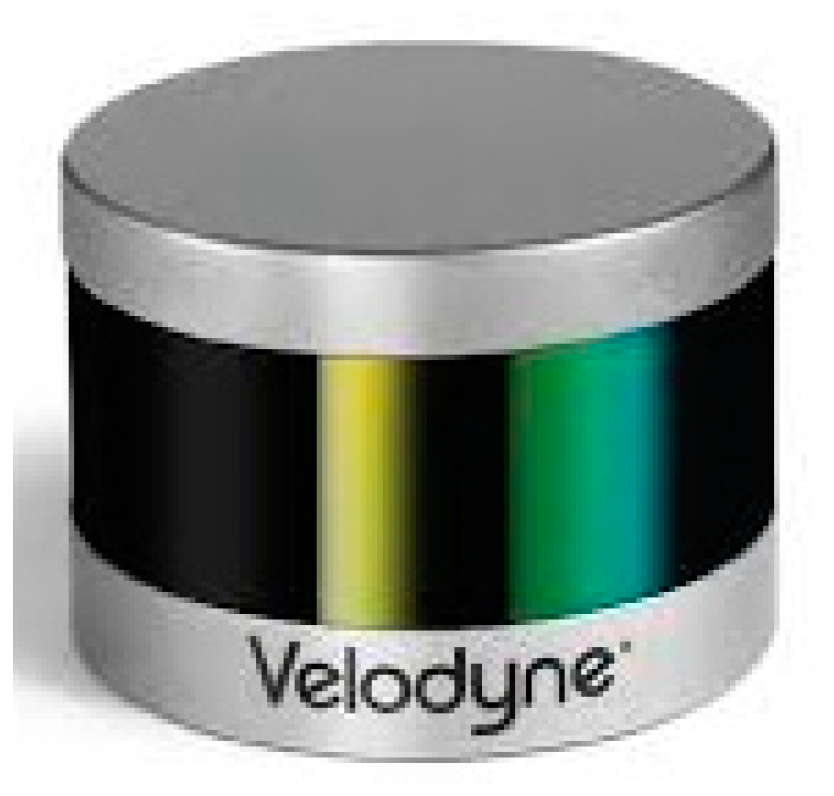
Two Velodyne VLP-16 (Figure 2) were mounted on the backpack system. Since its release in 2014, VLP-16 has been extensively utilized in mobile applications for both research and industry. The specifications of VLP-16 are summarized in Table 1. The sensor consists of 16 pairs of simultaneously rotating laser emitters and receivers within a compact sensor pod, and each laser has a fixed vertical angle of 2° resolution. The rotation rate varies from 5 to 20 Hz, with a set default value of 10 Hz, which gives 0.2° of horizontal angular resolution. Based on the default settings, VLP-16 rotates every 0.1 s and acquires approximately 28,800 points in each scan.
2.2. Inertial Sensor
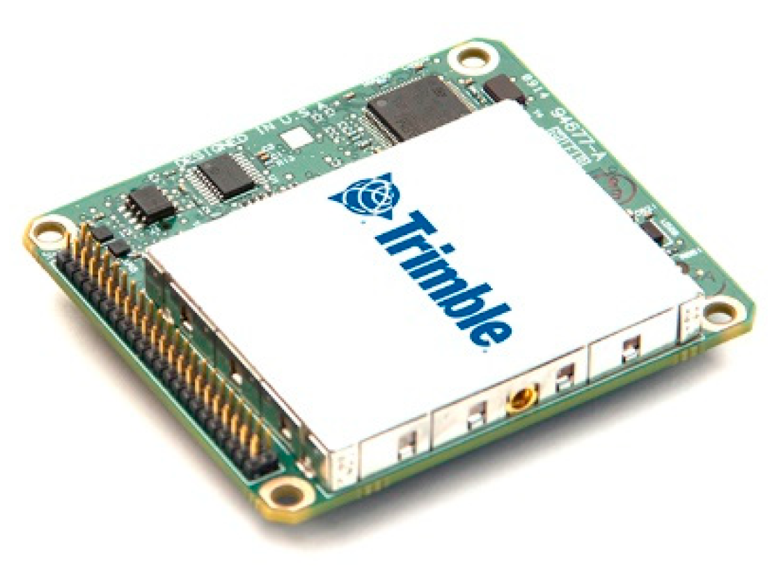
The Trimble APX-15 Unmanned Aerial Vehicle (UAV) was mounted for GNSS/INS. The Trimble APX-15 UAV (Figure 3) is an efficient GNSS-inertial solution for small UAVs. It weighs 60 g and is light enough to attach onto the backpack system. With GNSS signal integrated, APX-15 gives position, roll, pitch and heading output in 100 Hz, and IMU data in 200 Hz. This enables an accurate direct georeferencing of various sensor data. Detailed specifications of Trimble APX-15 UAV are described in Table 2.
2.3. Digital Cameras
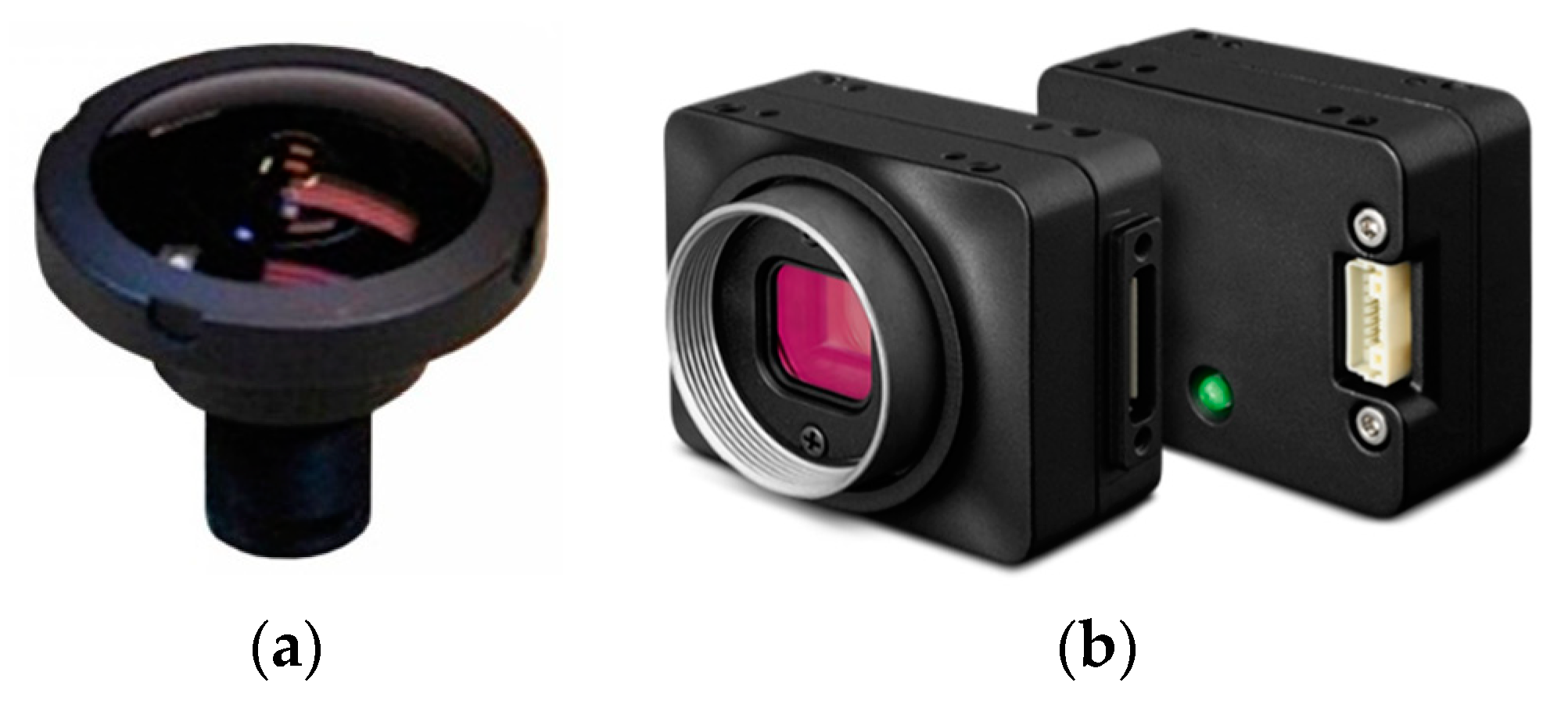
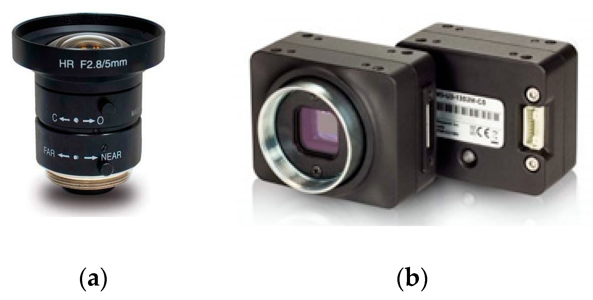
Four fisheye lens cameras and two perspective cameras were mounted on the backpack system. The model of the fisheye lens is Sunnex DSL315 and the camera body is Chameleon CM3-U3-32S4C (Figure 4). The camera has no shutter button, operating by receiving signals from a computing system. Detailed specifications of the fisheye camera are described in Table 3. Stereo cameras are also built in the backpack system. The perspective lens model is KOWA LM5JCM and the camera body is Chameleon CM3-U3-50S5C (Figure 5). Table 4 shows specifications of stereo camera.
3. Mathematical Models
3.1. Point Observation and Systematic Error Model of VLP-16
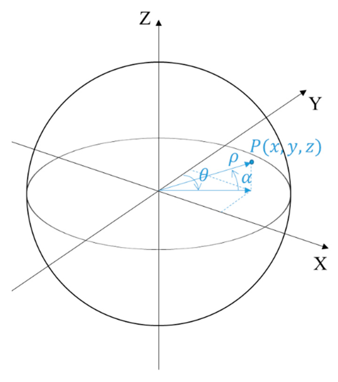
VLP-16 acquires range and horizontal angle measurements and provides fixed vertical angle for 16 laser channels (described in Section 2.1). The geometric relationship between spherical coordinates (, , ) and Cartesian coordinates (x, y, z) is shown in Figure 6. The formulas for converting spherical coordinates (, , ) to Cartesian coordinates (x, y, z) are given by Equation (1), where , , and are raw distance measurement, encoder angle measurements, and fixed vertical angle, respectively.
Sensor modelling is a crucial step in conducting rigorous self-calibration of laser scanners [33,34]. Numerous researchers have independently defined their own TLS error models. The error model of a laser scanner was estimated, and the accuracies of the estimated parameters were determined by comparing the measurements with an electronic distance measurement (EDM) [35]. A later model consists of about 20 additional parameters (APs) and can be found in [36]. This error model effectively modeled TLS instruments; however, it was defined for the AM-CW TLS, which uses a phase-based distance measuring system. In the case of MBL, laser emitter/receiver sets measure distance by a pulse-based Time of Flight (ToF) system with a fixed vertical angle. Therefore, AP terms should be different with phase-based TLS instruments. For Velodyne LiDAR, systematic error coefficients are defined by six parameters (i.e., range offset, scale error, horizontal angular offset, vertical angular offset, horizontal offset, and vertical offset) given by the manufacturer to model the deviations of measurements. Since the number of APs are multiplied by the number of lasers, the AP terms should be carefully chosen to avoid over-parameterization.
Although the manufacturer provides six parameters, some of the APs were neglected in this study. First, the estimation of scale error requires inclusion of an independent scale definition in the self-calibration network [36]. Range scale error cannot be estimated using the calibration approach and must therefore be estimated by other means, and independent baseline testing did not disclose the existence of this error [33]. In performing the tests, therefore, if scale error is included in the adjustment without an independent scale definition, an optimization process is not working properly. Considering there are no a priori known locations of the targets or scanner when performing in situ calibration, the scale error was therefore neglected. Horizontal offset and vertical offset were also fixed to maintain a higher accuracy of adjustment, for the following reasons: (1) Horizontal and vertical offset are highly correlated to the horizontal and vertical rotations, respectively [25,29]. In the case of VLP-16, the correlation coefficients of the parameters corresponding to the vertical and horizontal rotation corrections were found between 0.92 and 0.98, respectively [31]. (2) The vertical and horizontal alignments of each laser are precisely located according to the manufacturer-provided values set below the accuracy of the range observation. (3) Local coordinate error induced by horizontal and vertical offsets is not linearly dependent in the range observation.
Hence, the range offset, horizontal angular offset, and vertical angular offset were considered as APs in this study. Therefore, the point observation model for MBL could finally be determined as Equation (2). The coordinates of point at scan position j lying on plane k from laser n are related by rigid body transformation as given by:
where , , and denote a range observation, a horizontal angle observation, and a fixed vertical angle, while , , and indicate a range offset, a vertical angular offset, and a horizontal angular offset, respectively. is the rotation matrix which transforms the local coordinate system j to the reference coordinate system with the rotation angle about the X, Y and Z axes. is the translation from scan to the reference coordinate system.
3.2. Plane-Based Functional Model
Self-calibration of the laser scanner can be categorized according to the two major point- and plane-based methods. Point-based self-calibration uses center point coordinates extracted from a number of signalized targets through numerous estimation and transformation processes. Point-based self-calibration using TLS such as Trimble GS200 and GX can be found in [37,38]. In addition, research has been studied to determine the optimal network design for correlation mitigation and to achieve good parameterization of TLS self-calibration [39,40,41]. One limitation of such calibration approaches includes manual installation of signalized targets, which is labor-intensive and can decrease the accuracy of point-based self-calibration due to high parameter correlation [42]. Moreover, in the case of multi-beam laser scanners, extracting the exact target points is almost impossible due to the fixed vertical angle.
Meanwhile, point coordinates on the surface of planar targets can be used directly instead of center point coordinates of signalized targets. Since signalized targets are not required, plane-based self-calibration is one of the most widely adopted methods. The main advantage of plane-based self-calibration is that the plane parameters within each plane can be estimated in the adjustment model, thereby mitigating the need to measure an accurate reference target and enhancing the method’s applicability for in situ calibration. Skaloud and Lichti [43] presented a rigorous approach to bore-sight self-calibration of an airborne laser scanning system by conditioning the geo-referenced LiDAR points to fit into common plane surfaces. However, the objective of their work was more oriented to the estimation of extrinsic parameters between the Inertial Measurement Unit (IMU) and the LiDAR unit, considering only range offset as AP. Bae and Lichti [34] conducted plane-based self-calibration with scan data using FARO 880. In their study, self-calibration simulations investigated various scanner configurations, and the results demonstrated that a long baseline between two scan stations enables a more accurate estimation of collimation axis errors. Also, plane-based calibration has been reported to offer almost the same performance as point-based calibration when conducted under a strong network configuration [44]. The self-calibration approach in this study is based on the plane-based functional model of [34]. This model estimates not only exterior orientation parameters (EOPs) and APs, but also plane parameters, simultaneously. The plane-based method can remove the necessity of calibration target set-up and reference target coordinate measurement using additional sensors. The condition equation associated with parameters and observations can be expressed by the plane-based functional model as given by:
where are the direction cosines of the normal vector of the plane k, and is the orthogonal distance from the origin of the reference coordinate system to the plane k. The direction cosines must satisfy the unit length constraint:
3.3. Least Squares Solution
The combined adjustment model (Gauss–Helmert adjustment model) was used, since the objective function includes inseparable observations and parameters, and each function includes more than one observation. Details on the implementation of the Gauss–Helmert adjustment model can be found in [43]. Therefore, only the quantities of the adjustment will be discussed herein.
First, the VLP-16 provides two observations for each point: a range and a horizontal angle. For unknown parameters, three APs were considered for each laser as aforementioned, and six rigid body transformation parameters for each scan must be included to combine all scanner coordinate systems into a reference coordinate system. Lastly, a unit length condition must be constrained to the equation for each plane. For the network constraint, according to [45], either the ordinary minimum or the inner constraint for the datum definition has no opposing impact on the accuracy of self-calibration. Since the scale is defined by range observations, the ordinary minimum constraint, which fixes the EOPs of the first scan to define the datum as the reference coordinate system, was chosen in this study. In addition, not all 16 laser angular offsets can be estimated simultaneously, because a certain amount of angular offset for every laser can be compensated by sensor orientation, causing a problem when defining the scanner space. Therefore, horizontal and vertical angular offsets for one laser are held fixed. Assuming that we have i points located on k planes from n lasers in j scans in the adjustment, the least squares solution can be summarized as in Table 5.
4. Experiment Description and Result Analysis
Calibration experiments were designed using simulated and real datasets. All the experiments were performed by the following process. First, the point cloud for each scan location was captured by defining the “frame”, as MBL completes one rotation and covers 360° of the horizontal field of view. Next, plane fitting using Maximum Likelihood Estimation SAmple Consensus (MLESAC) for all point clouds was processed [46]. Each point lying on its surface has a plane number and parameters. Common planes that are mutually detected in all point clouds are manually matched to the reference scan. Least squares adjustment and accuracy assessment follow.
4.1. Simulation Experiments
Since the zero-order design problem—the datum problem—has been addressed by fixing the EOPs of the reference scan as aforementioned, the first-order design problem—the configuration problem—is our interest. Several network configuration conditions were considered to determine the minimum network configuration for plane-based self-calibration of the backpack-based MBL system. These include: (1) the number and configuration of scans; (2) the size, the number, and the configuration of incorporated planes; (3) the minimum number of points lying on the planar surface. In order to determine the minimum network configuration suitable for the backpack-based MBL system in situ self-calibration, simulation experiments were designed with respect to those two significant conditions. Simulation environments were designed by changing the size of the test site and sensor configurations using our own developed simulator program. All the simulated datasets have 0.2° horizontal angle increments, and the same systematic errors. The given systematic errors for the simulation data are shown in Table 6. Random noises were set to 0.003 m, and 0.01° for range and angle observations, respectively.
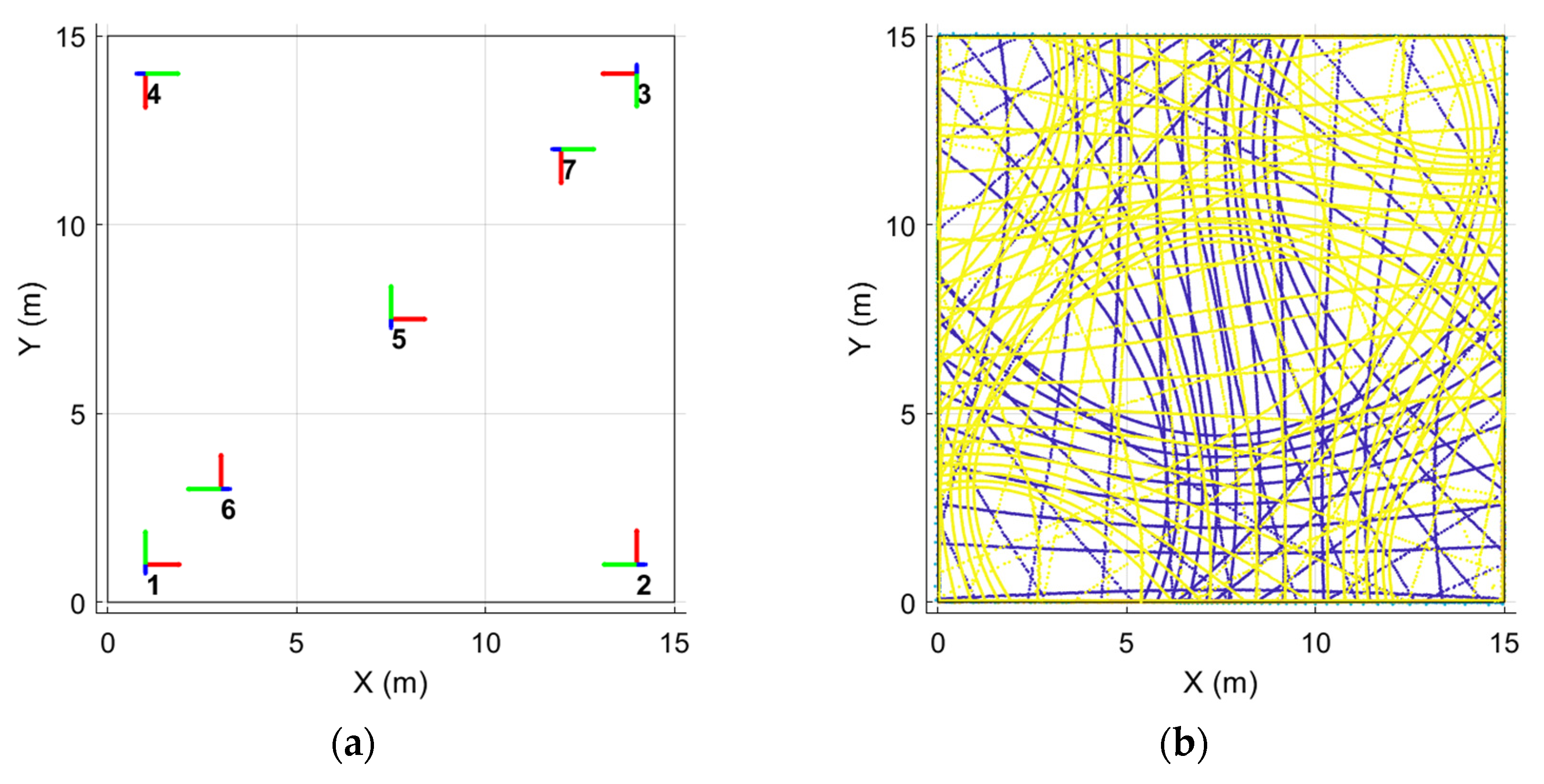
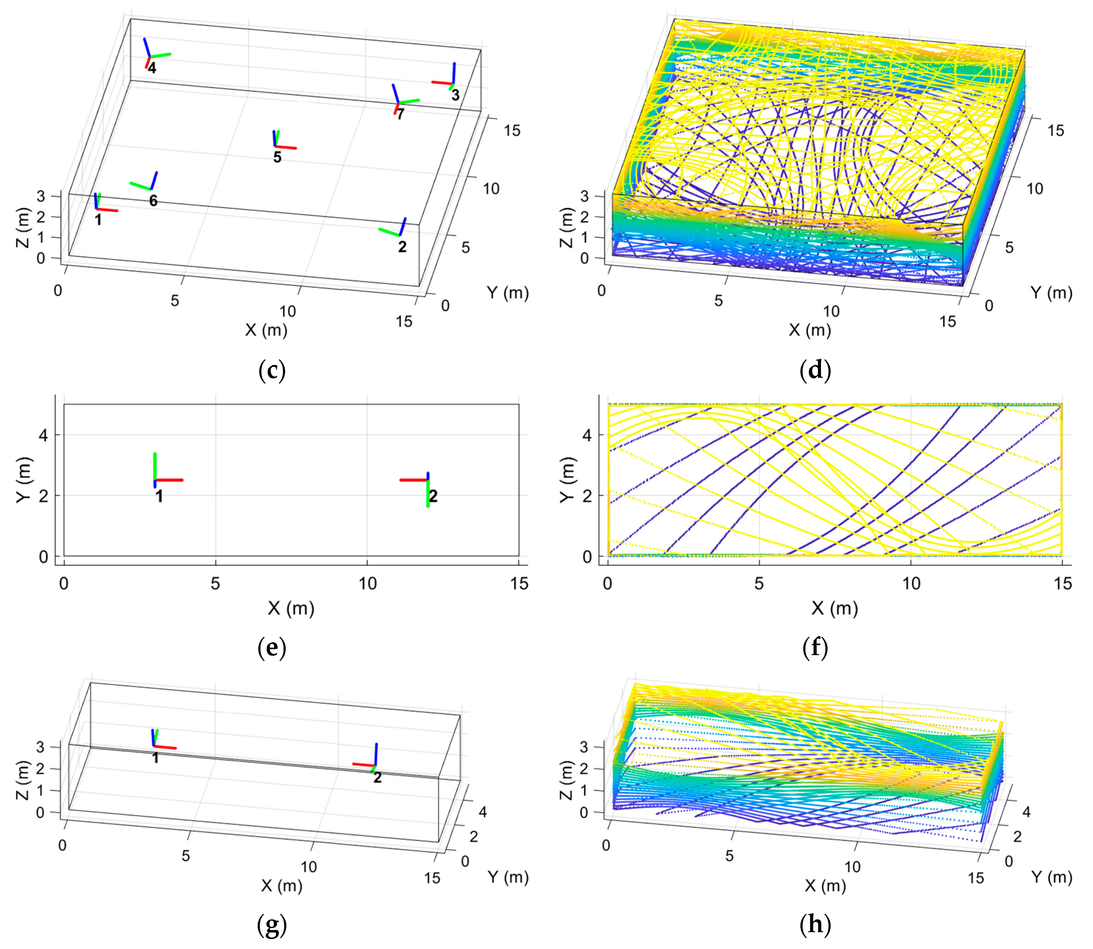
The first experiment (Calibration I) was conducted by reducing the number of scans successively to determine the optimal configuration and the minimum number of scans required. As shown in Figure 7a,c, the size of the test site was firstly set to 15 m × 15 m × 3 m, and four scans were located at the corner, two scans were located near the corner, and one was located at the center. This full network configuration, including seven scans and six planes, was constructed based on [45]. Each scan was slightly tilted along the X axes (omega in orientation parameters) for better estimation of the adjustment [42]. Figure 7b,d show the point cloud generated for Calibration I.
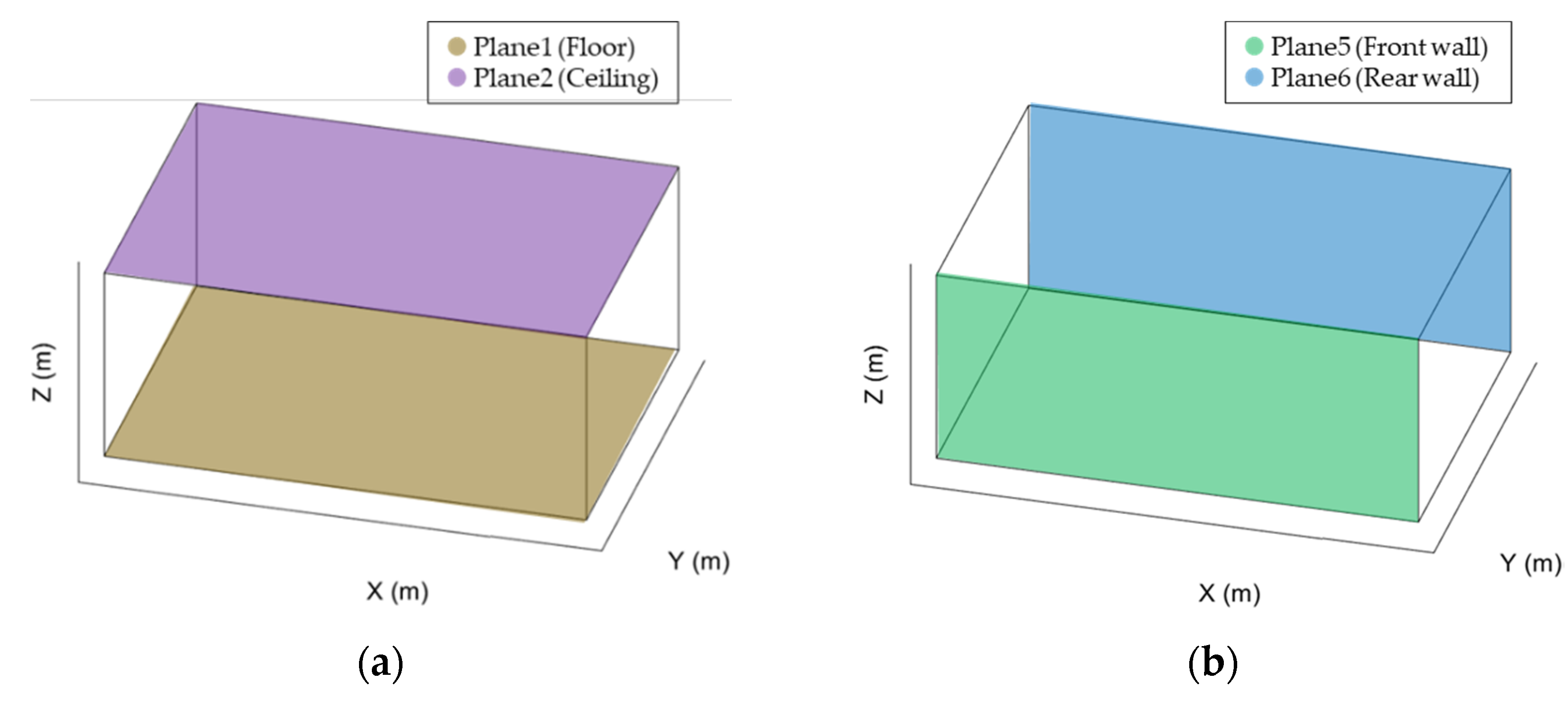
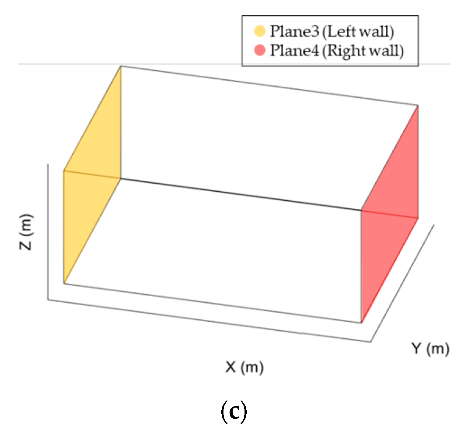
For the second experiment (Calibration II), as described in Figure 7e,g, the dataset was firstly generated in a 15 m × 5 m × 3 m corridor-shape environment, and the length of the corridor was shortened by 1 m successively until it reached 7 m × 5 m × 3 m in order to investigate the effective dimensions of the room for the self-calibration. After the investigation, the number of incorporated planes also reduces to determine the minimum number of planes required. Figure 7f,h show the point cloud generated for Calibration II. Figure 8 describes the assigned number for each plane.
For the third experiment (Calibration III), the number of points used in the adjustment reduces to identify the minimum requirement of the redundancy for the adjustment.
4.2. Analysis of Simulation Experiment Results
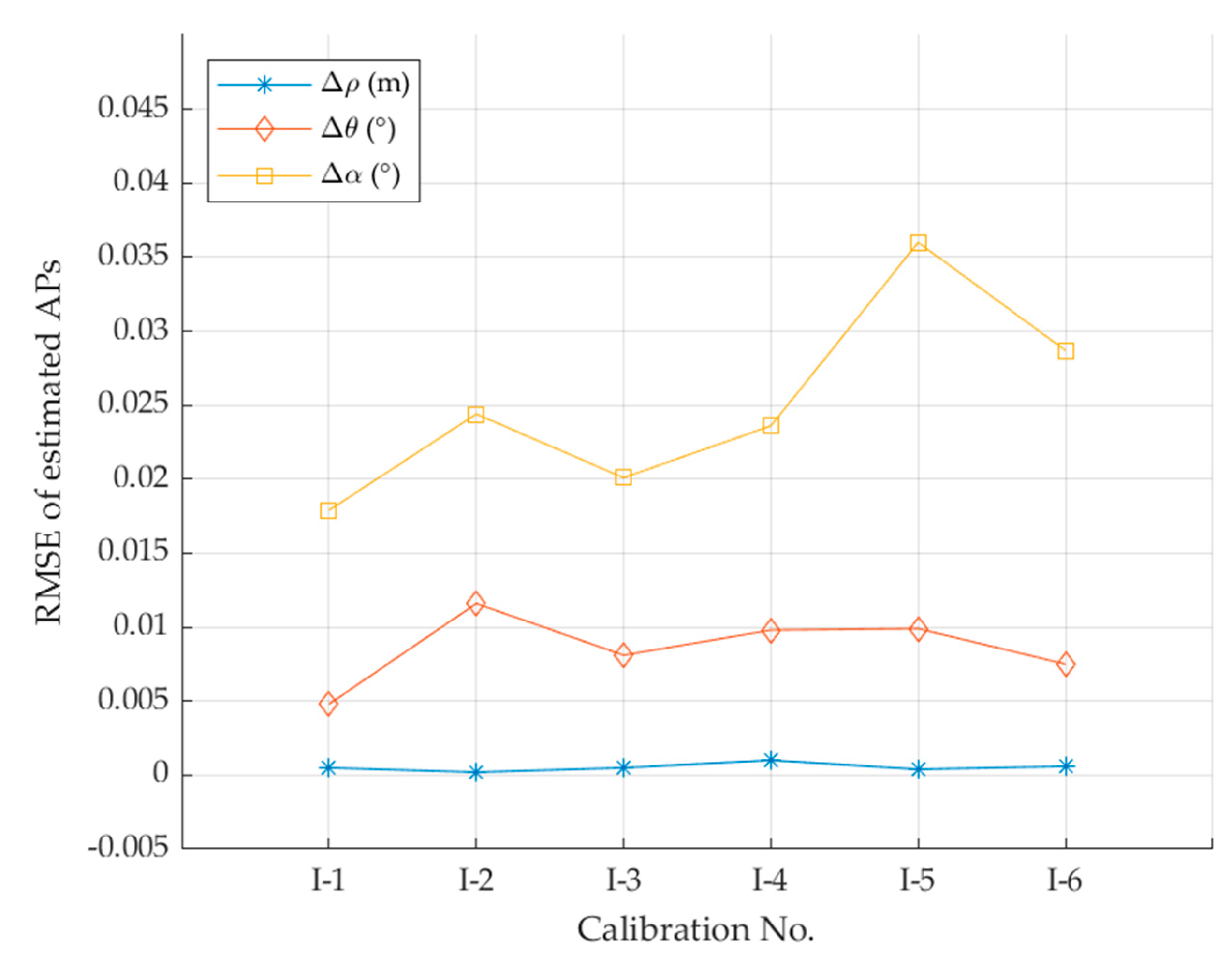
In the first experiment (Calibration I), the number of scans was reduced successively. Table 7 provides a summary of the first experiment. Also, please refer to Figure 7a–d and Figure 8. The RMSE between estimated and given AP values are plotted in Figure 9. As can be seen, all the tests show high similarity. The asymmetry network configuration of Calibration I-2 might have affected the accuracy of the adjustment. For Calibration I-5, the scan location was too close to the corner, leading to a high incidence angle to the planes. High incidence angle observation tends to deteriorate the overall accuracy of the adjustment [25]. The results from the first experiments indicate that there is no significant change of accuracy when using only two scans compared with the full network, which uses seven scans. For the rest of the experiments, therefore, only two scans (not too close to the corner) were used for self-calibration.
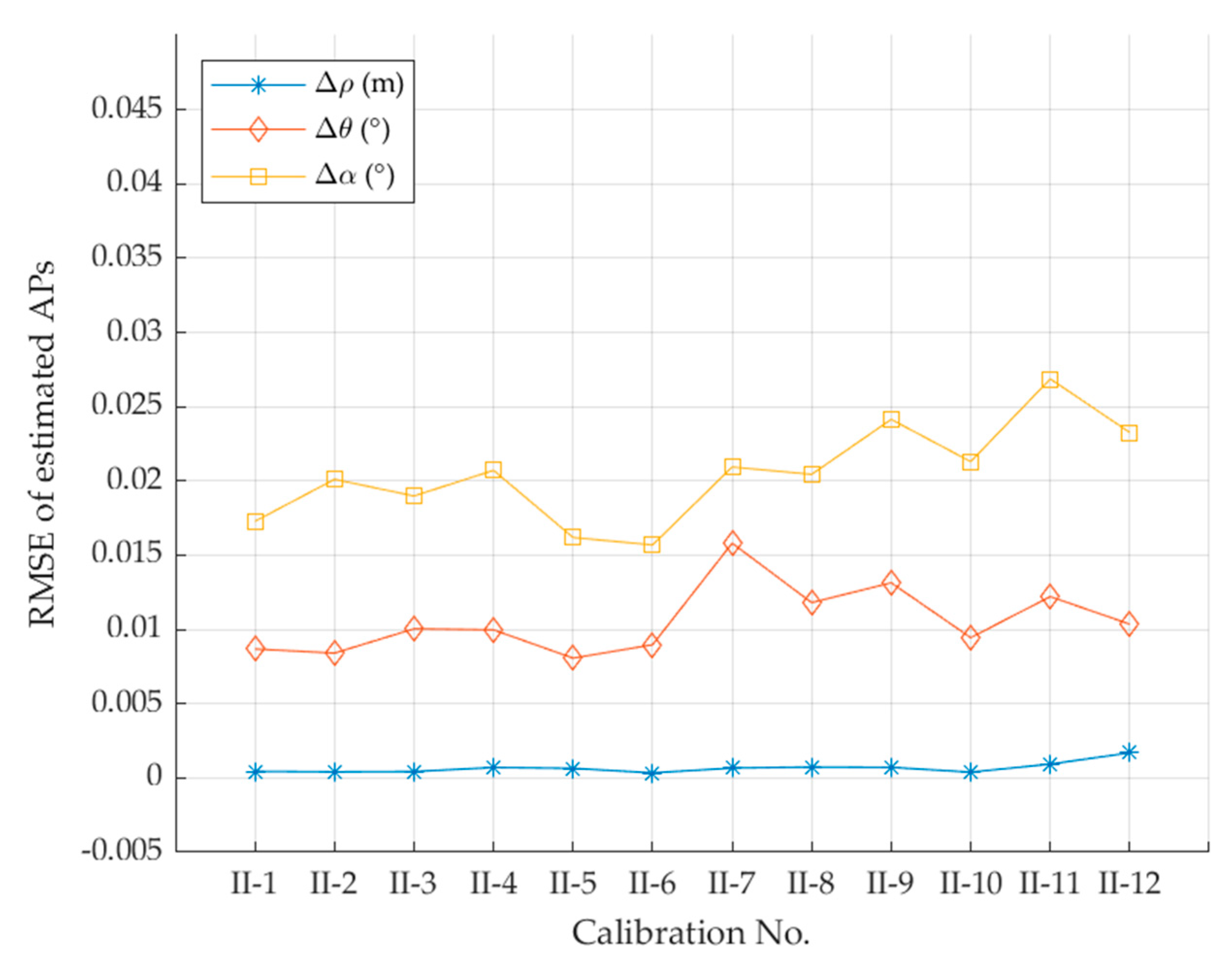
Following the result from Calibration I, the second experiment (Calibration II) used only two scans for self-calibration by decreasing the dimensions of the room and the number of incorporated planes. Also, please refer to Figure 7e–h and Figure 8. Table 8 summarizes the information on Calibration II. The length of the test site decreased until 7 m. The scan locations were about 3 m apart from the wall and 1 m from each other. Except for Calibration II-13 and II-14, the remaining twelve experiments have calibration solutions. The RMSEs of the estimated APs for the twelve experiments are provided in Figure 10. The range offset showed consistent RMSE values for all experiments, while the two angular offsets showed a slight variance. Even the reduced dimension of the test site (i.e., 7 m × 5 m × 3 m) with three planes (i.e., ceiling and two orthogonal walls) provided a low level of RMSE values as seen in Figure 10.
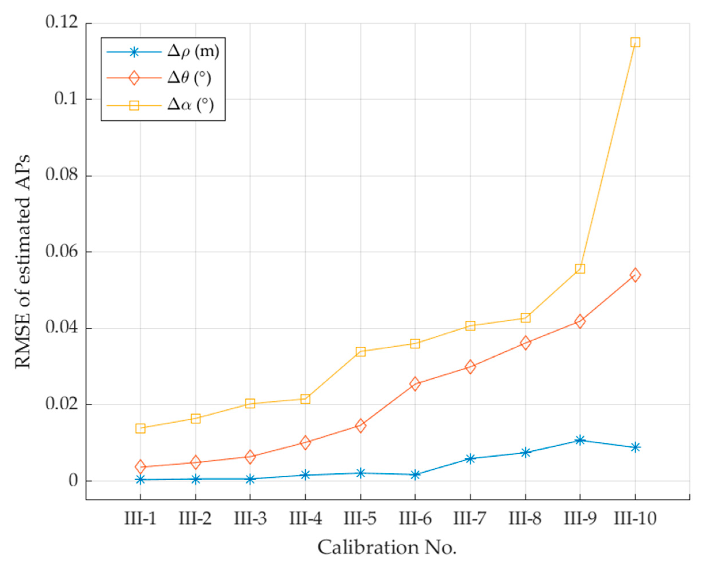
Following the result from Calibration II-12, the third experiment (Calibration III) was conducted by reducing the number of points in the adjustment. In Table 9, the summary of Calibration III is presented. The reduction rate varied from 50 to 99%, which gave the number of used points as 11,275 to 226. The redundancy linearly reduced as the number of points decreased.
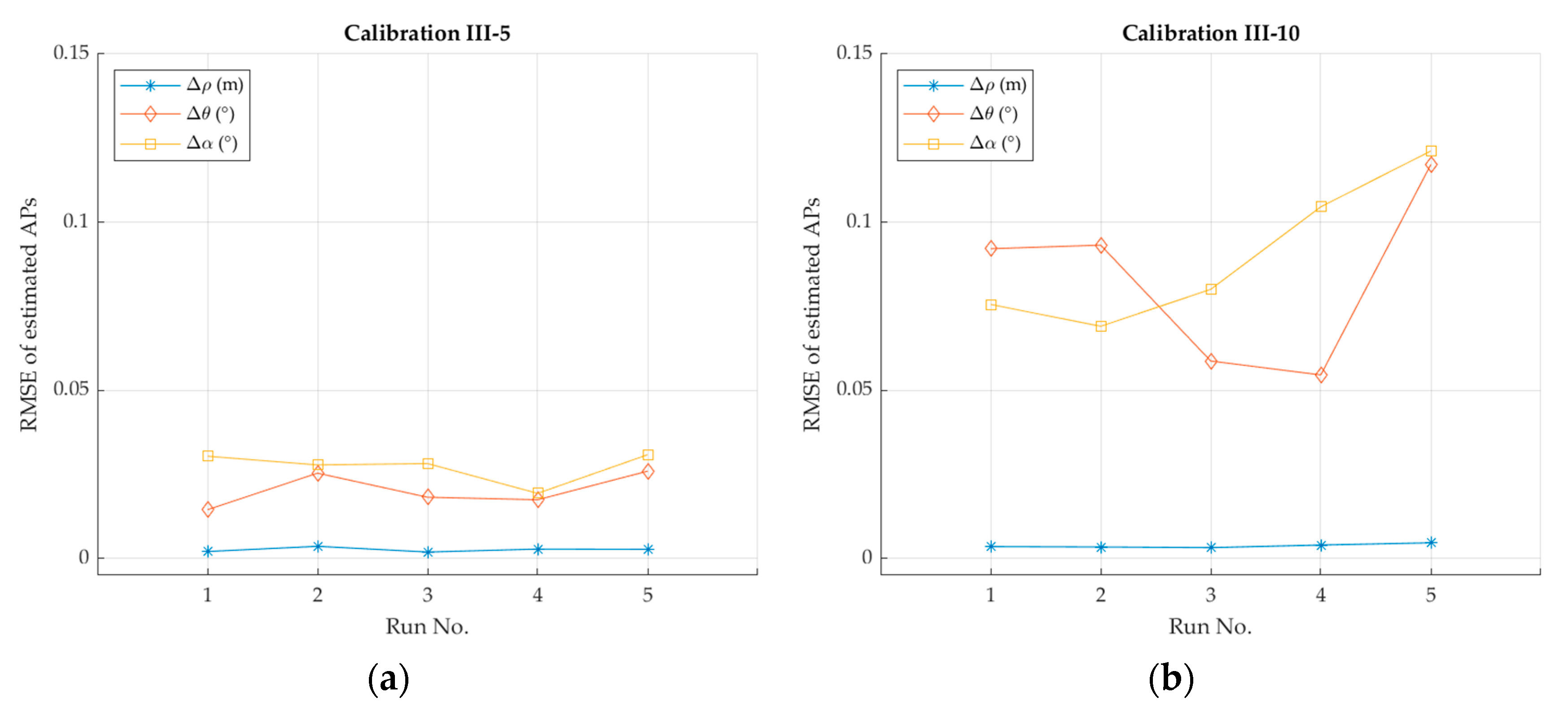
As shown in Figure 11, a clear inverse relationship between the RMSE of the estimated parameters and the number of used points was found. We also found that there were dramatic increases in RMSE for angular offsets from Calibration III-9 to III-10, while range offset showed a relatively small increase. To further investigate this phenomenon, additional calibration tests were repeatedly conducted. More specifically, Calibration III-10 (using 226 points) ran five times. At this stage, one should note that the involved number of points was kept as 226 but the points were randomly picked from the whole dataset (i.e., from 22,550 points) for each run. For the comparison, Calibration III-5 (using 2255 points) ran five times as well while picking the involved points randomly for each run. Calibration III-5 was chosen because it corresponded to the inflection point as seen in Figure 11. The results of these additional tests were shown in Figure 12. In the case of repetition of Calibration III-5 (in Figure 12a), RMSE values of the estimated APs for five runs were very similar and the variance of the values was low. On the other hand, repetition of Calibration III-10 (in Figure 12b) showed fluctuating RMSE results, which were too many dataset-dependent outcomes. After these additional tests, it was found that if the number of used points was too small, the calibration process provided unreliable solutions. In this regard, at least 2000 or more points is recommended to estimate reliable angular offsets.
4.3. Kinematic Self-Calibration
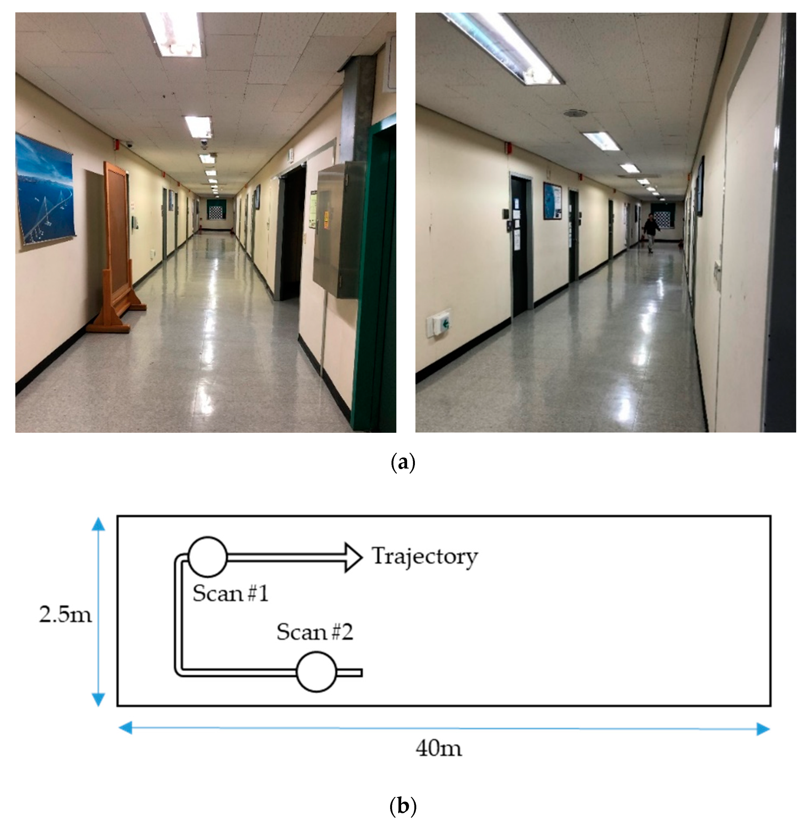
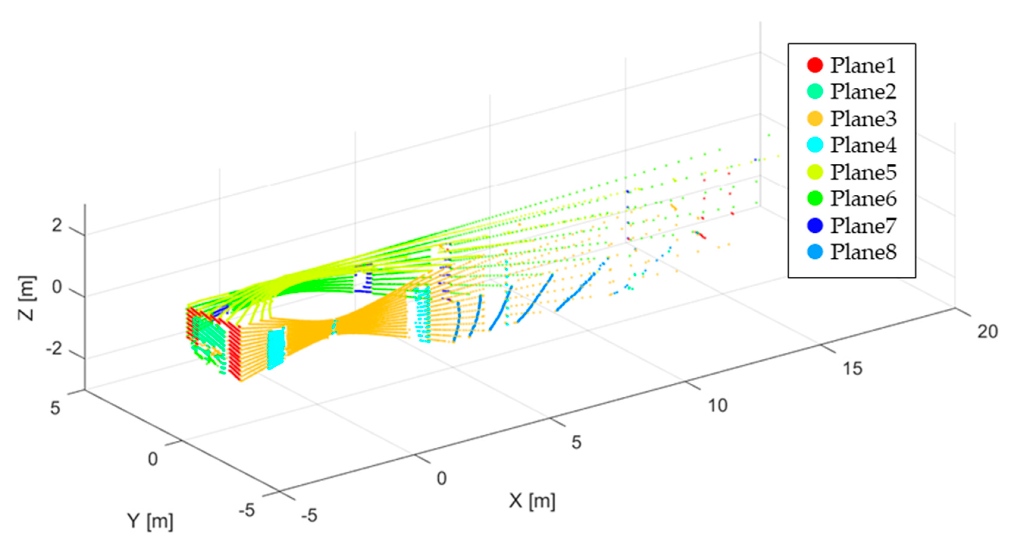
Based on the results of the simulation tests, a real dataset was captured using the backpack system. The data acquisition site is a corridor of approximate 2.5 m × 40 m × 2.5 m dimensions (Figure 13a). To test the performance of the kinematic in situ self-calibration of the backpack-based MBL system, the user wore the backpack system and walked along the corridor to acquire point clouds. A schematic drawing of the data acquisition site and trajectory are also provided in Figure 13b. As can be seen, two scan locations were selected from whole trajectory. The first scan was captured near the corner, and the second scan was captured apart from the first scan. The omega angle of each scan was slightly tilted, and the kappa angle was rotated by 180°. Then, planar feature extraction and the matching process were carried out using two scan datasets. Figure 14 describes the planar features commonly seen in both scans, which include six vertical planes and two horizontal planes. A total of eight planes were identified, including walls, doors, a window, the floor, and the ceiling.
4.4. Analysis of Kinematic Self-Calibration Results
Experiments using the real dataset were conducted to implement the minimum network configuration for the kinematic self-calibration found on the above analysis. Two experiments were conducted to investigate the accuracy when the full and minimum network configurations were used. First, Calibration IV-1 was conducted including all eight planes and 8140 points. Calibration IV-2 was also performed for comparison with Calibration IV-1. Three planes (ceiling and two orthogonal walls) and 2308 points were used for the self-calibration. A summary of the two experiments is presented in Table 10.
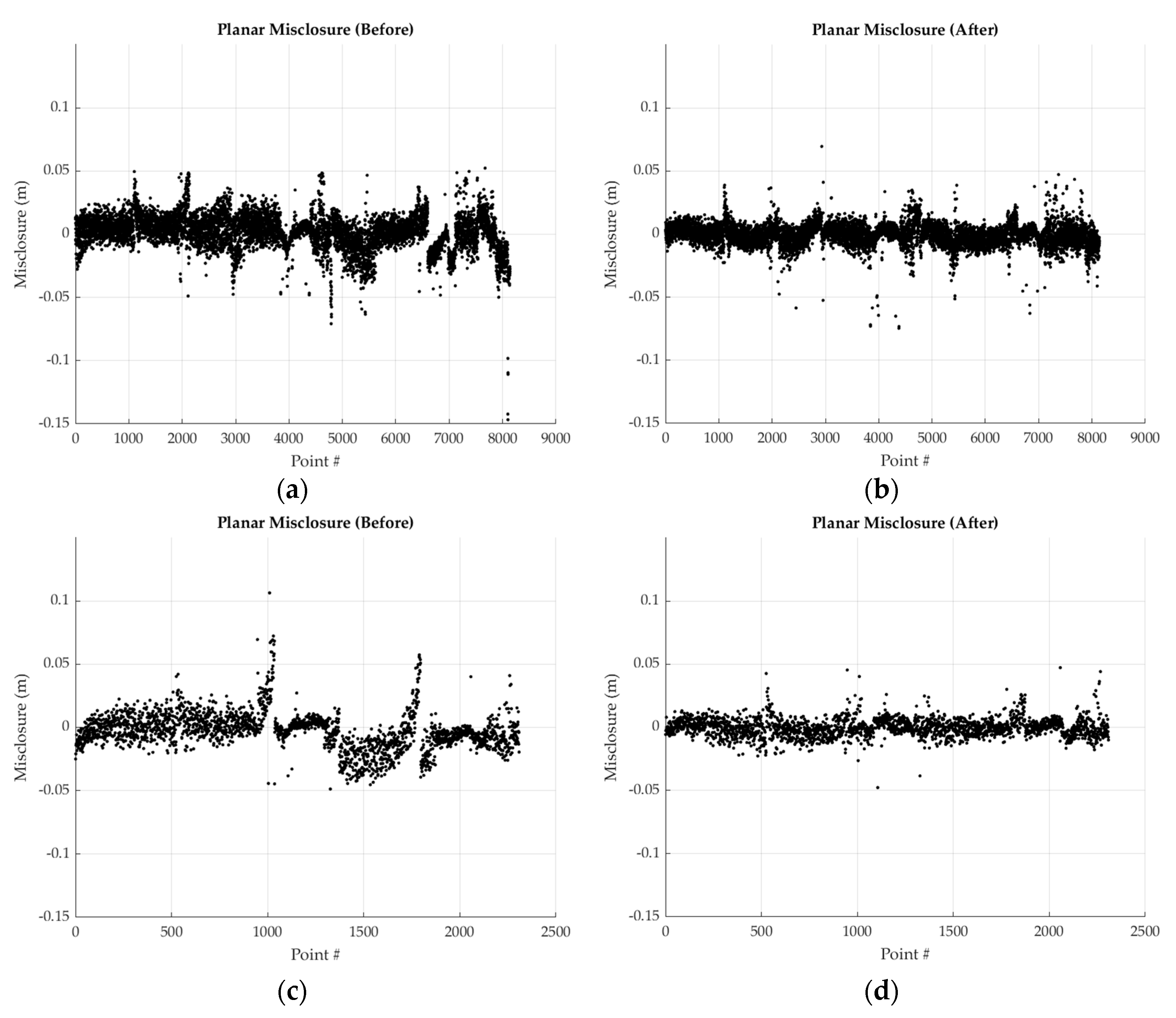
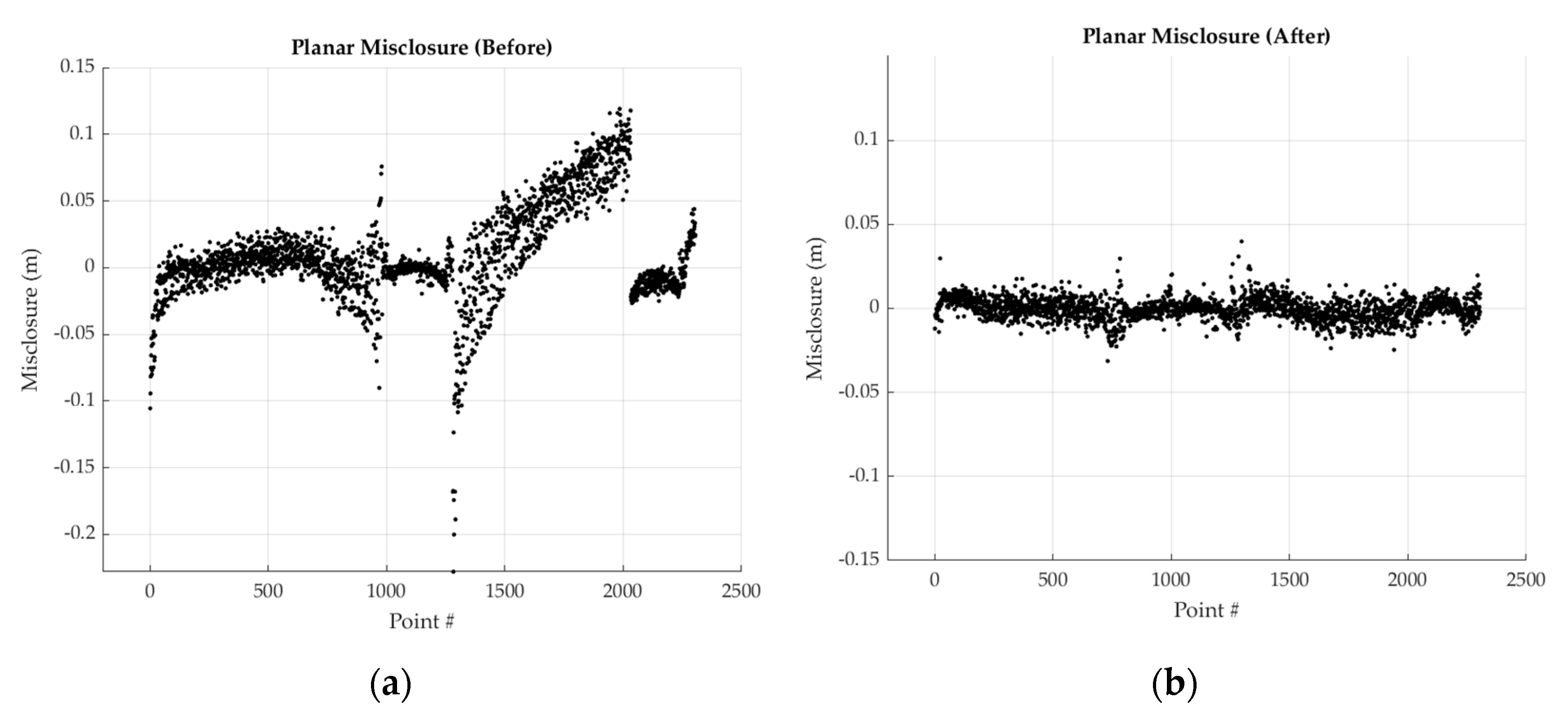
For accuracy evaluation of the kinematic self-calibration, planar misclosure vectors were examined to confirm that the self-calibration had effectively modeled the sensor. For planar misclosure calculations, parameters other than APs were held to the same values in order to compare the results from self-calibration. The planar misclosure results before and after adjustment are given in Figure 15.
As can be seen, in both cases, the systematic errors were not completely removed after the adjustment. Nevertheless, the results of both cases showed improvements of planar misclosure RMSE by 35.7 and 53.3% after the adjustment. The RMSE of Calibration IV-2 was even lower than that of Calibration IV-1. This is reasonable, as more outliers were included in the Calibration IV-1 dataset. A summary of the results regarding planar misclosure can be found in Table 11.
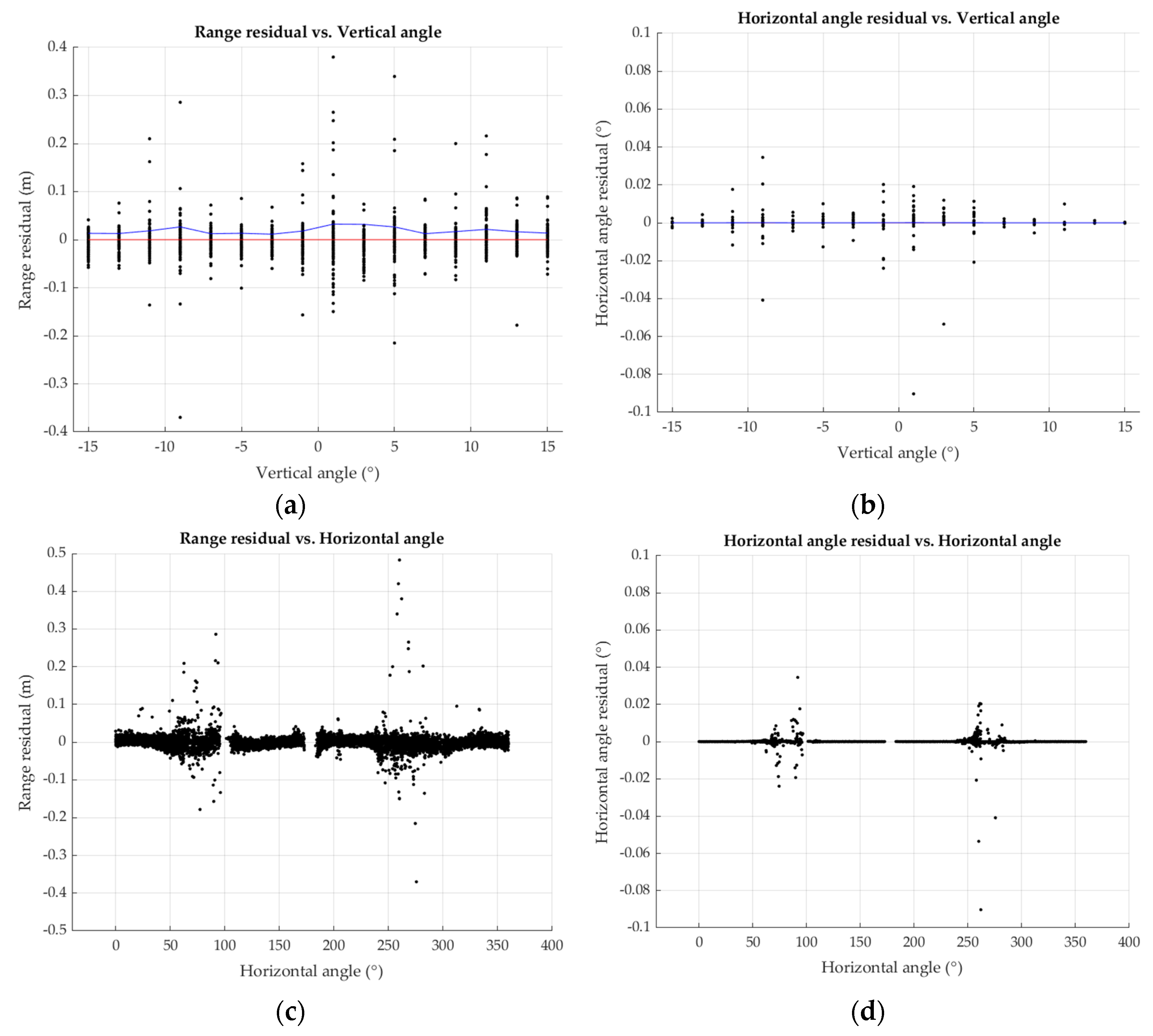
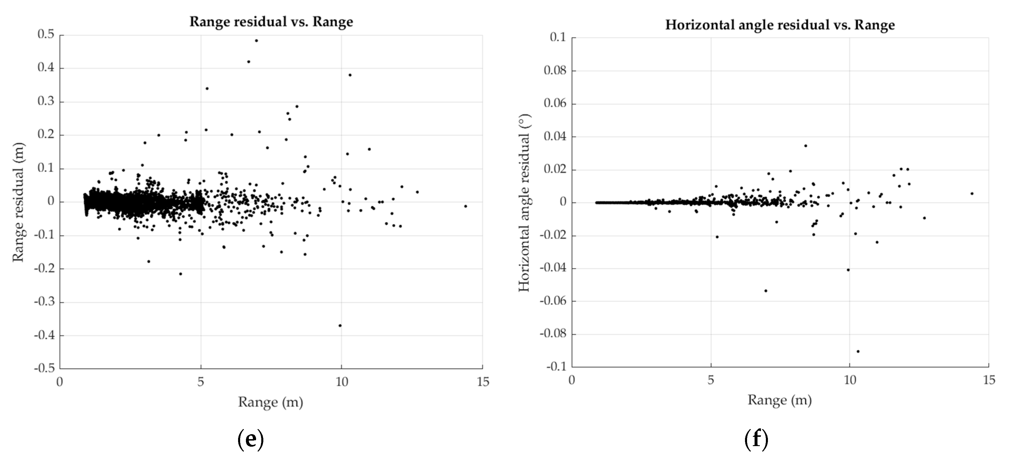
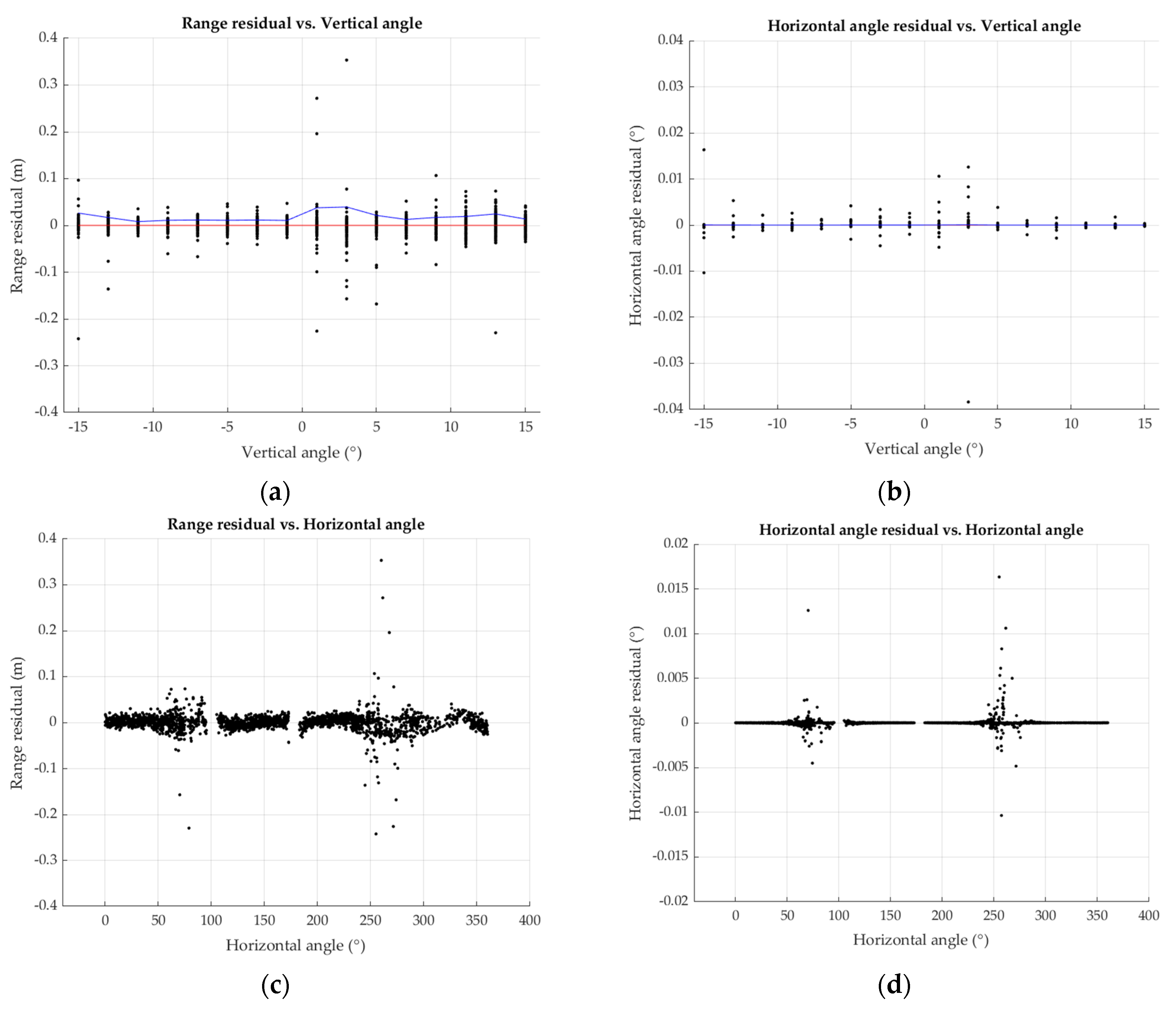
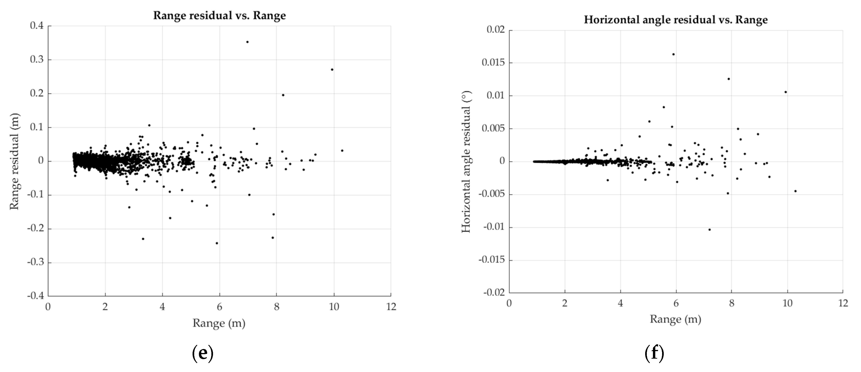
In order to further investigate the existence of systematic trends, observation residuals from the adjustment were also examined. Figure 16 and Figure 17 describe two observation residuals (a range and a horizontal angle) versus vertical angle, horizontal angle, and range for Calibration IV-1 and IV-2, respectively. For both cases, similar unmodelled systematic errors still existed in the observation residual. Residuals versus vertical angle showed no trends of systematic effects, as the mean residual values with respect to laser elevation angle had zero values (refer to Figure 16a,b and Figure 17a,b). On the other hand, residuals versus horizontal angle showed large variations at 90° and 270°, which are the directions of high incidence angles to the walls (refer to Figure 16c,d and Figure 17c,d). This was expected from simulation tests and previous studies in the literature. For the final analysis for residuals, residuals versus range were plotted (refer to Figure 16e,f and Figure 17e,f). As can be seen, outliers increased as range increased, in both the range and horizontal angle observations.
Furthermore, the reliability of the estimated parameter could be presumed by examining the correlation coefficients between the estimated parameters. The correlation coefficients between the APs and EOPs are presented in Table 12 and Table 13. The correlations between the EOPs and APs were averaged over all of the lasers with one EOP, and the correlations between APs were averaged over all lasers with the same laser. In general, correlations between the EOPs were higher than the correlations between the EOPs and the APs. The moderate (not significantly strong) correlation values were, also, found between and , and , and and . They were marked in bold in the tables. This correlation between and the orientation parameters was likely due to the small number of points with respect to the horizontal plane (floor and ceiling), and, moreover, the amount of tilting angle was not sufficient for perfectly de-coupling between the translation and orientation parameters. Nevertheless, it should be noted that the estimated parameters did not have strong correlations and were derived reliably.
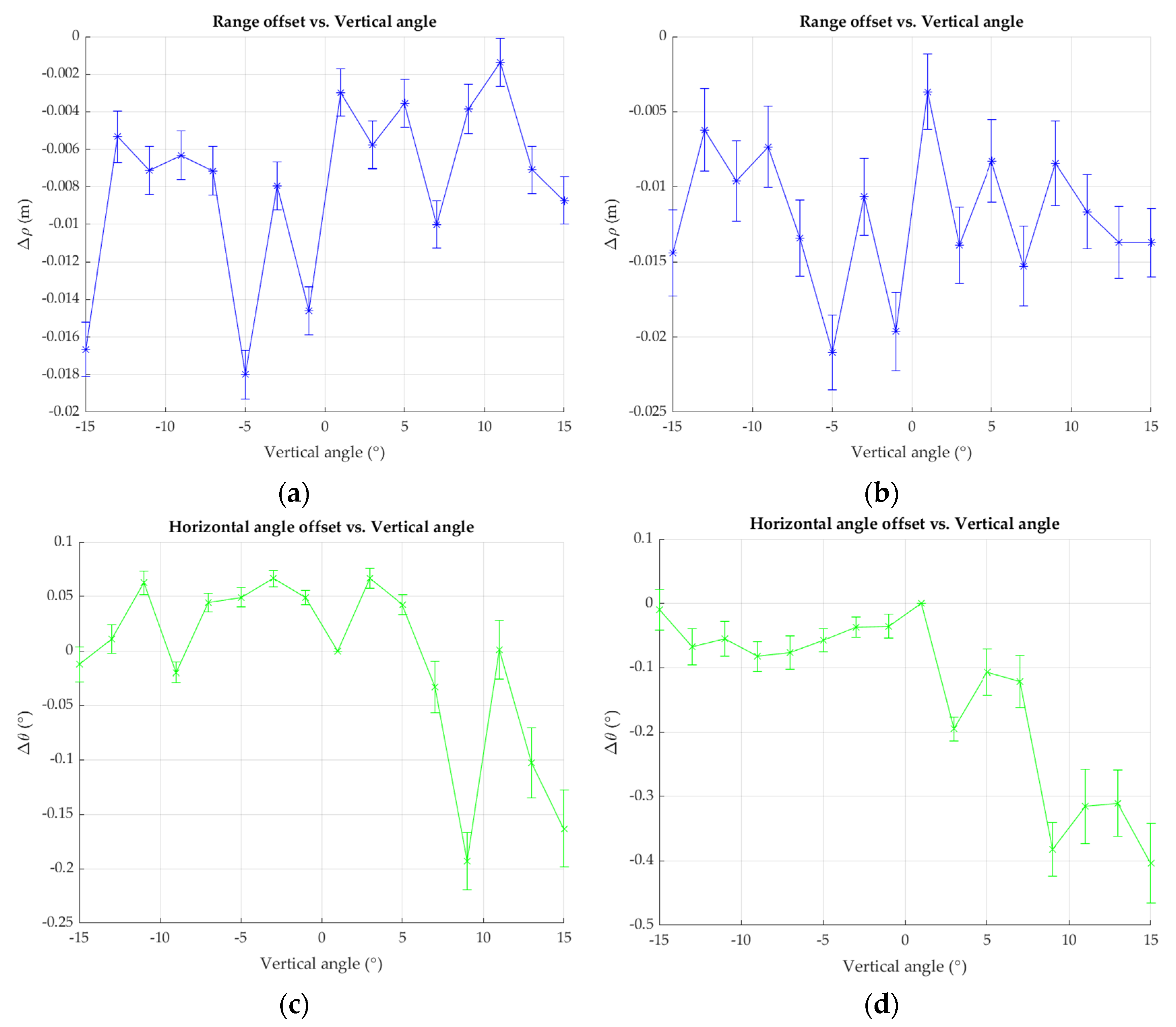
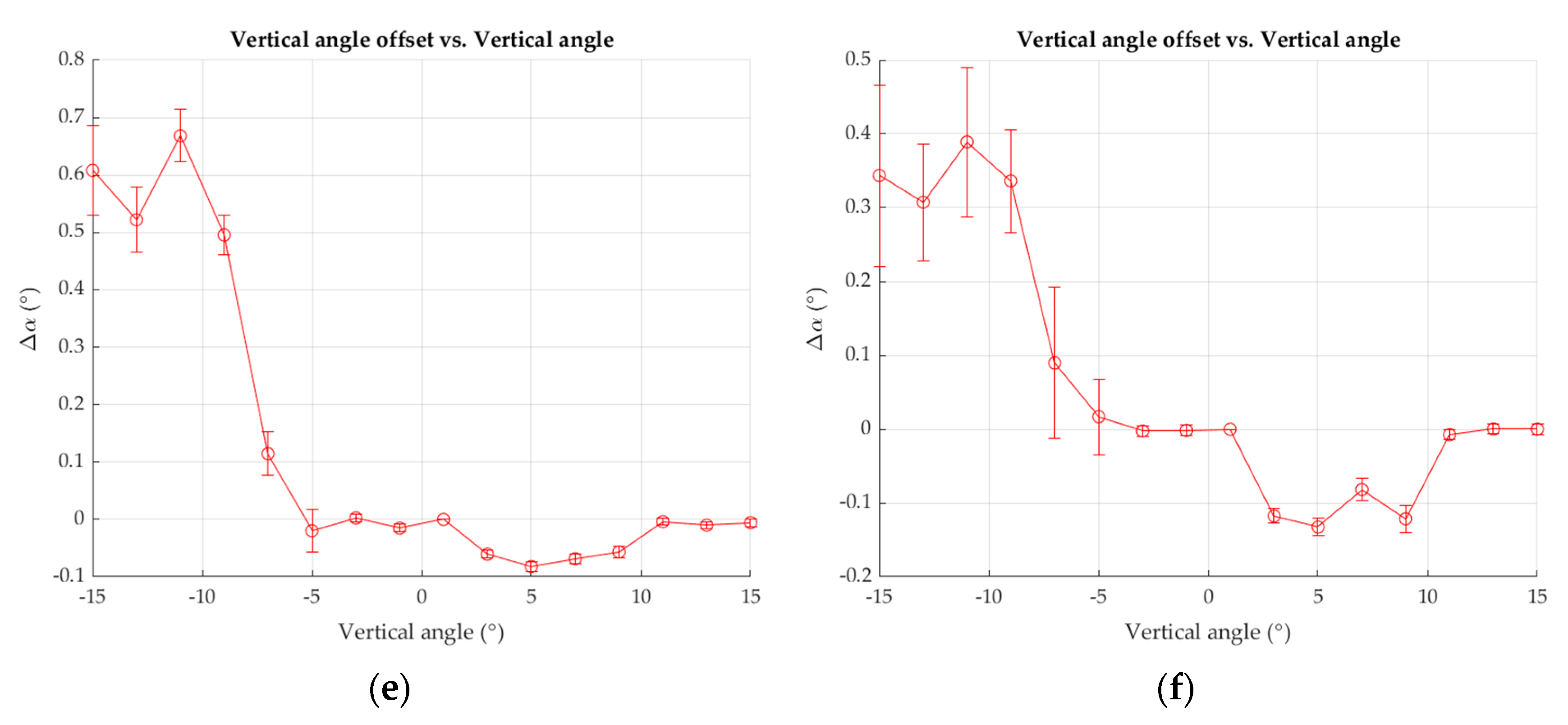
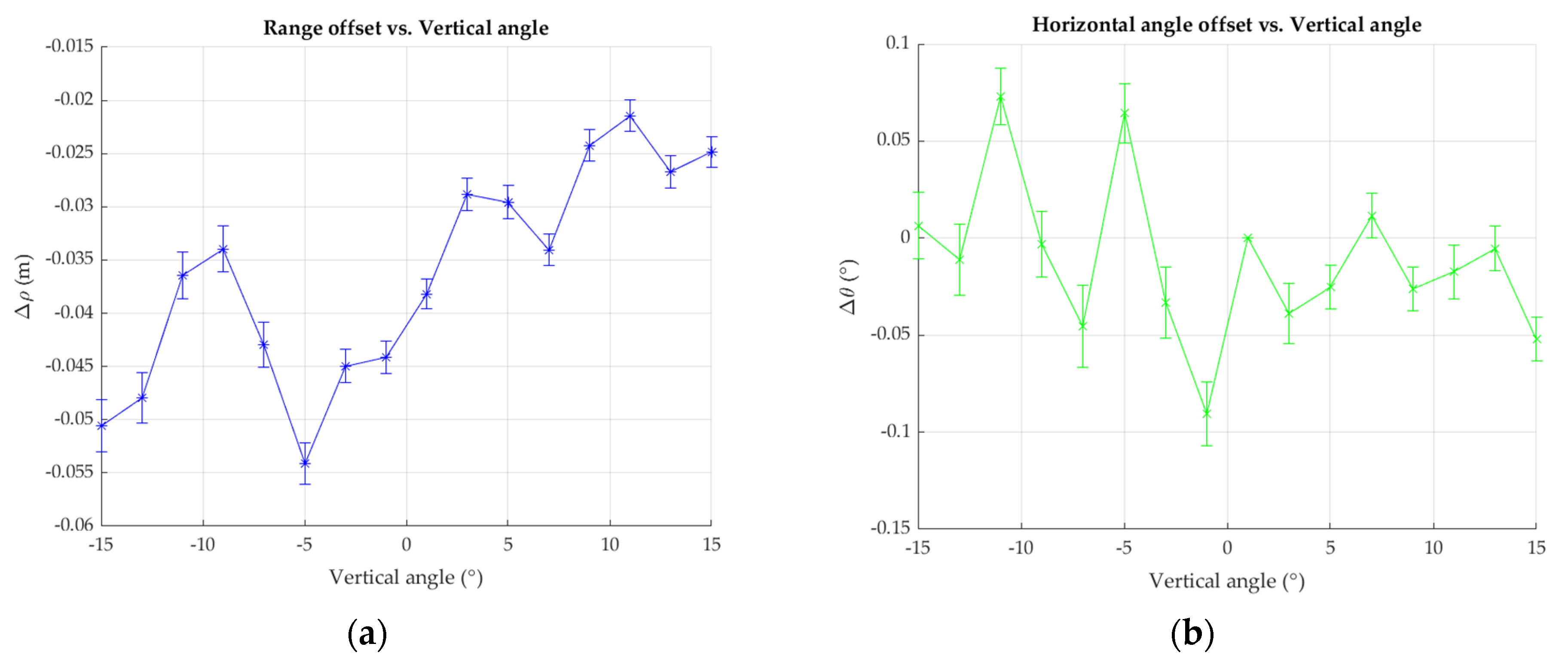
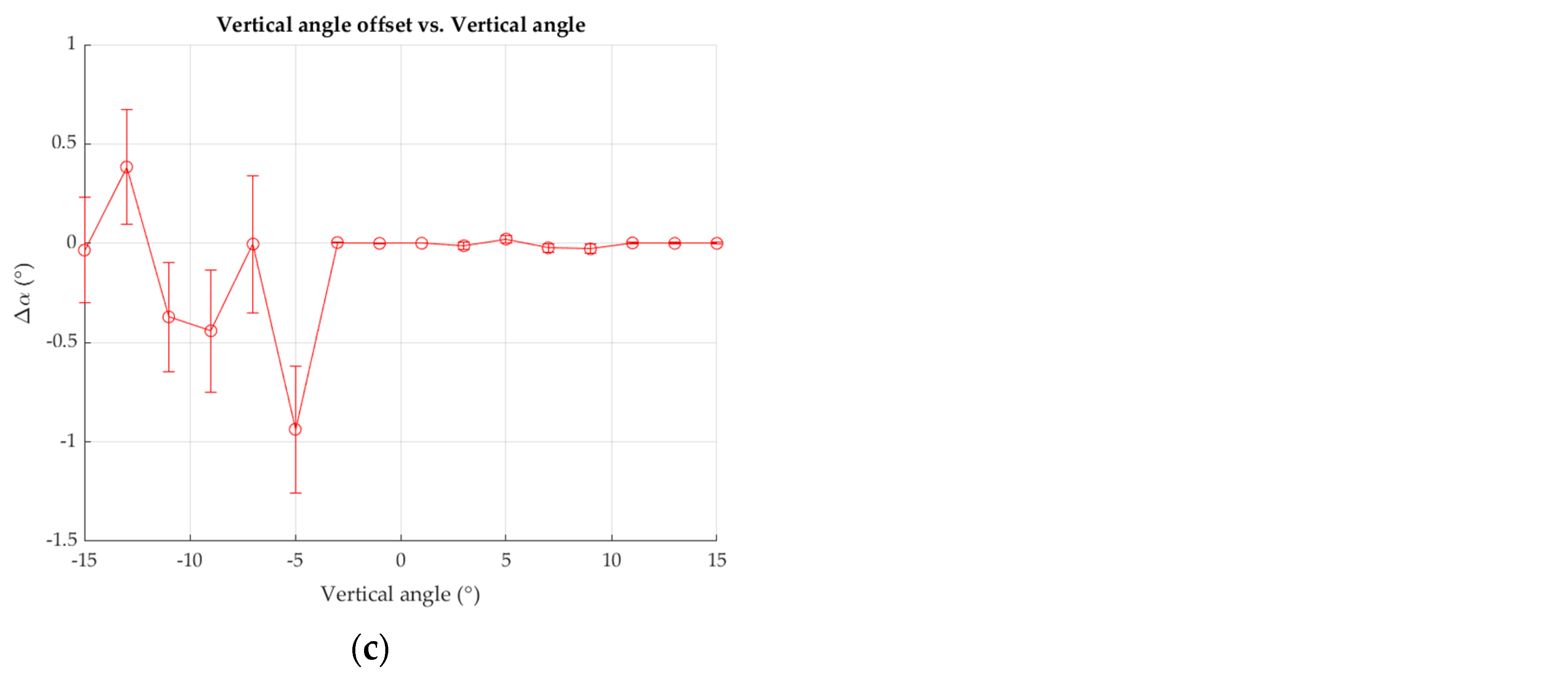
Based on the results from Calibration IV-1 and IV-2, the estimated AP values and their standard deviations for all the lasers are plotted in the function of the vertical angle in Figure 18. Both calibrations demonstrated similar results of parameter estimation, while the estimation of parameters with respect to the directed high vertical angle laser showed different results. As can be seen, the standard deviations of horizontal angular offset for directing a high vertical angle laser were high, while the standard deviations of the vertical angular offset were low. The horizontal and vertical angular offsets for laser 1 (having 1 of vertical angle) were held fixed as zeros, as mentioned in Section 3.3. Estimated parameters for Calibrations IV-1 and IV-2 are provided in Table 14. The EOP estimation showed reasonable standard deviations relative to the estimated values. As similarly investigated in Section 4.2, kinematic calibration of the backpack-based MBL system can be performed using a minimum network configuration with reasonable accuracy in a real environment.
4.5. Temporal Stability Analysis of Kinematic Self-Calibration
An additional experiment (Calibration V) was conducted for temporal stability analysis. About one month later after performing self-calibration (Calibration IV), we re-calibrated the same sensor under the similar condition. More specifically, the data acquisition site and the rest of the conditions were identical to the Calibration IV for comparison. Based on the findings from the previous analysis, the minimum network configuration was considered for Calibration V. Summary of Calibration V is given in Table 15.
Table 16 shows the summary of planar misclosure before and after Calibration V. The planar misclosure results before and after Calibration V are, also, given in Figure 19. As can be seen, the RMSE of planar misclosure before the calibration (i.e., 0.038 m) increased compared to Calibration IV-2 (i.e., 0.015 m). In addition, estimated AP values from Calibration V can be found in Figure 20, showing different values compared to Calibration IV-2 (Figure 18b,d,f). On the other hand, RMSE of planar misclosure after Calibration V (i.e., 0.007 m in Table 16) showed a similar result to Calibration IV-2 (i.e., 0.007 m in Table 11). Through this additional experiment, we found that the APs of the MBL system were changing unstably over time, and the calibration process provided a stable level of planar misclosure RMSE.
5. Discussion
In this section, the effectiveness of the proposed self-calibration method is discussed in terms of accuracy, time, and cost. First, a comparative analysis between the previous MBL self-calibration approaches and the proposed one is carried out. Table 17 shows the performances (i.e., accuracy and improvement) of five representative MBL calibration approaches and the proposed one. At this stage, one should note that a direct comparison of the performances among different approaches is almost impossible since their sensor systems, methods, datasets, environments, computational performances are all different. Nevertheless, the comparison in Table 17 shows the overall performances of the approaches. Although there is a variance in the type of MBL sensors, our method achieved a fair improvement (35–81%) compared to other results. In particular, Glennie [29] and Chan and Lichti [30] performed kinematic calibrations of MBL mounted on a vehicle platform. In these approaches, the RMSEs of planar misclosure after the calibration were 0.023 and 0.014 m, respectively, which are higher than the proposed case. This is due to the fact that vehicle moving speed is much faster than human walking speed, causing a higher measurement noise level. The proposed approach showed a similar (or somewhat better) level of RMSE to the static calibrations.
Secondly, the proposed kinematic self-calibration of the backpack-based MBL system can significantly reduce time and cost compared to the traditional target-based static calibrations. The proposed one does not need an installation of targets and tripods to fix the scan location since it is aiming for kinematic in situ calibration. Although the proposed method is not fully automatic, the running time of the whole process takes up to 30 s (under the condition of 2 scans, 3 planes, and around 2000 points), except for the manual plane matching. The computer processor is an AMD Ryzen 5 1600 six-core processor with DDR-4 16GB 1500MHz of RAMs. The program for the whole process is written in MATLAB. The program and the algorithm are not yet optimized, and the processing time can be improved in the future study.
6. Conclusions
This study investigated kinematic in situ self-calibration to frequently re-calibrate the backpack-based MBL system using on-site data for handling unstable measurements of the sensor. In order to determine the minimum network configuration for kinematic self-calibration, simulation experiments were conducted beforehand. First, a full network of the simulated datasets was generated, and self-calibrations were performed by reducing the number of scans, the size of the test site, the number of incorporated planes, and the number of points. The accuracies of the experiments were analyzed by examining the RMSE of the estimated APs to determine the minimum network configuration. The results of the simulation experiments show relatively stable performance with a minimum network configuration of at least two scans, three planes that are orthogonal to each other, and around two thousand points used. Based on this preliminary analysis, kinematic self-calibration using real datasets was then performed. The datasets were acquired while the user was wearing a backpack system and walking along a corridor. The accuracy of kinematic self-calibration was evaluated by investigating the planar misclosure, measurement residuals, correlation coefficients, and estimated parameters and their standard deviations. The results demonstrate that the kinematic self-calibration of the backpack-based MBL system could improve the point cloud accuracy with the RMSE of planar misclosure up to 81%. Moreover, the effectiveness of the proposed approach in terms of time and cost was also addressed.
After the various experiments and analysis using the proposed kinematic in situ self-calibration of the backpack-based MBL system, the contributions of this study can be summarized as follows. First, self-calibration of MBL was analyzed with respect to various network configurations. The minimum network configuration for the kinematic in situ self-calibration of the backpack-based MBL system and its performance were found through various experiments. Secondly, the kinematic in situ self-calibration of the backpack-based MBL system can perform using on-site datasets, reaching the higher accuracy of point cloud. In addition, this research can serve as a guideline for users who require the self-calibration of a backpack-based MBL system to improve overall accuracy and to generate point cloud data for precise mapping or surveying. Future studies will mostly focus on: (1) the development of real-time automatic plane matching for automatic in situ calibration; (2) outlier removal during the iteration of least squares based on statistical analysis to maximize calibration accuracy.
Author Contributions
H.S.K. was responsible for developing the methodology and writing the original manuscript, C.K. provided the backpack system, Y.K. helped revise the manuscript, and K.H.C. supervised the research. All authors have read and agreed to the published version of the manuscript.
Funding
This work was supported by a National Research Foundation of Korea (NRF) grant (no. 2019R1A2C1011014) funded by the Korean government (MSIT).
Informed Consent Statement
Not applicable.
Data Availability Statement
Data sharing not applicable.
Acknowledgments
The authors are grateful to C2L Equipment (www.c2l-equipment.com) for helping to develop the backpack system for this research.
Conflicts of Interest
The authors declare no conflict of interest.
References
- Bosché, F.; Ahmed, M.; Turkan, Y.; Haas, C.T.; Haas, R. The value of integrating scan-to-BIM and scan-vs-BIM techniques for construction monitoring using laser scanning and BIM: The case of cylindrical MEP components. Autom. Construct. 2015, 49, 201–213. [Google Scholar] [CrossRef]
- Cole, D.M.; Newman, P.M. Using laser range data for 3D SLAM in outdoor environments. In Proceedings of the 2006 IEEE International Conference on Robotics and Automation (ICRA), Orlando, FL, USA, 15–19 May 2016; pp. 1556–1563. [Google Scholar]
- Wu, Y.; Kim, H.; Kim, C.; Han, S.H. Object recognition in construction-site images using 3D CAD-based filtering. J. Comput. Civ. Eng. 2009, 24, 56–64. [Google Scholar] [CrossRef]
- Shih, N.J.; Huang, S.T. 3D scan information management system for construction management. J. Const. Eng. Manag. 2006, 132, 134–142. [Google Scholar] [CrossRef]
- Tang, P.; Anil, E.B.; Akinci, B.; Huber, D. Efficient and Effective Quality Assessment of As-Is Building Information Models and 3D Laser-Scanned Data. In Proceedings of the International Workshop on Computing in Civil Engineering 2011, Miami, FL, USA, 12–22 June 2011; pp. 486–493. [Google Scholar]
- Park, H.S.; Lee, H.M.; Adeli, H.; Lee, I. A new approach for health monitoring of structures: Terrestrial laser scanning. Comp. Aid. Civ. Inf. Eng. 2007, 22, 19–30. [Google Scholar] [CrossRef]
- Yang, H.; Xu, X.; Neumann, I. Laser scanning-based updating of a finite-element model for structural health monitoring. IEEE Sens. J. 2015, 16, 2100–2104. [Google Scholar] [CrossRef]
- Riveiro, B.; Lindenbergh, R. Laser Scanning: An Emerging Technology in Structural Engineering; CRC Press: Boca Raton, FL, USA, 2019; pp. 1–3. [Google Scholar]
- Halterman, R.; Bruch, M. Velodyne HDL-64E lidar for unmanned surface vehicle obstacle detection. In Proceedings of the Unmanned Systems Technology XII, Orlando, FL, USA, 6–9 April 2010; Volume 7692, p. 76920D. [Google Scholar]
- Moosmann, F.; Stiller, C. Velodyne SLAM. In Proceedings of the IEEE Intelligent Vehicles Symposium 2011, Baden-Baden, Germany, 5–9 June 2011; pp. 393–398. [Google Scholar]
- Geiger, A.; Lenz, P.; Urtasun, R. Are we ready for autonomous driving? The kitti vision benchmark suite. In Proceedings of the 2012 IEEE Conference on Computer Vision and Pattern Recognition (CVPR), Providence, RI, USA, 16–21 June 2012; pp. 3354–3361. [Google Scholar]
- Choi, K.H.; Kim, Y.; Kim, C. Analysis of Fish-Eye Lens Camera Self-Calibration. Sensors 2019, 19, 1218. [Google Scholar] [CrossRef] [Green Version]
- Jozkow, G.; Toth, C.; Grejner-Brzezinska, D. Uas Topographic Mapping with Velodyne Lidar Sensor. ISPRS Ann. Photogramm. Remote Sens. Spat. Inf. Sci. 2016, III-1, 201–208. [Google Scholar] [CrossRef]
- Chen, T.; Dai, B.; Liu, D.; Song, J.; Liu, Z. Velodyne-based curb detection up to 50 m away. In Proceedings of the 2015 IEEE Intelligent Vehicles Symposium, Seoul, Korea, 28 June–1 July 2015; pp. 241–248. [Google Scholar]
- Hess, W.; Kohler, D.; Rapp, H.; Andor, D. Real-time loop closure in 2D LIDAR SLAM. In Proceedings of the 2016 IEEE International Conference on Robotics and Automation (ICRA), Stockholm, Sweden, 16–21 May 2016; pp. 1271–1278. [Google Scholar]
- Ravi, R.; Lin, Y.J.; Elbahnasawy, M.; Shamseldin, T.; Habib, A. Bias impact analysis and calibration of terrestrial mobile lidar system with several spinning multibeam laser scanners. IEEE Trans. Geosci. Remote Sens. 2018, 56, 5261–5275. [Google Scholar] [CrossRef]
- Shamseldin, T.; Manerikar, A.; Elbahnasawy, M.; Habib, A. SLAM-based Pseudo-GNSS/INS Localization System for Indoor LiDAR Mobile Mapping Systems. In Proceedings of the IEEE/OIN PLANS 2018, Monterey, CA, USA, 23–26 April 2018. [Google Scholar]
- Leica Pegasus: Backpack Wearable Mobile Mapping Solution. Available online: https://leica-geosystems.com/products/mobile-sensor-platforms/capture-platforms/leica-pegasus-backpack# (accessed on 29 December 2020).
- Viametris. Available online: https://www.viametris.com/backpackmobilescannerbms3d (accessed on 29 December 2020).
- GreenValley International. Available online: https://greenvalleyintl.com/hardware/libackpack/ (accessed on 29 December 2020).
- Gexcel Geomatics & Excellence. Available online: https://gexcel.it/en/solutions/heron-mobile-mapping (accessed on 31 December 2020).
- Velas, M.; Spanel, M.; Sleziak, T.; Habrovec, J.; Herout, A. Indoor and Outdoor Backpack Mapping with Calibrated Pair of Velodyne LiDARs. Sensors 2019, 19, 3944. [Google Scholar] [CrossRef] [Green Version]
- Chow, J.C. Multi-Sensor Integration for Indoor 3D Reconstruction. Ph.D. Thesis, University of Calgary, Calgary, AB, Canada, April 2014. [Google Scholar]
- García-San-Miguel, D.; Lerma, J.L. Geometric calibration of a terrestrial laser scanner with local additional parameters: An automatic strategy. ISPRS J. Photogramm. Remote Sens. 2013, 79, 122–136. [Google Scholar] [CrossRef]
- Glennie, C.; Lichti, D.D. Static calibration and analysis of the velodyne HDL-64E S2 for high accuracy mobile scanning. Remote Sens. 2010, 2, 1610–1624. [Google Scholar] [CrossRef] [Green Version]
- Muhammad, N.; Lacroix, S. Calibration of a Rotating Multi-Beam Lidar. In Proceedings of the IEEE /RSJ International Conference on Intelligent Robots and Systems (IROS), Toulouse, France, 18–22 October 2010; pp. 5648–5653. [Google Scholar]
- Atanacio-Jiménez, G.; González-Barbosa, J.-J.; Hurtado-Ramos, J.B.; Francisco, J.; Jiménez-Hernández, H.; García-Ramirez, T.; González-Barbosa, R. Velodyne HDL-64E calibration using pattern planes. Int. J. Adv. Robot. Syst. 2011, 8, 70–82. [Google Scholar] [CrossRef]
- Chen, C.-Y.; Chien, H.-J. On-site sensor recalibration of a spinning multi-beam LiDAR system using automatically-detected planar targets. Sensors 2012, 12, 13736–13752. [Google Scholar] [CrossRef] [Green Version]
- Glennie, C. Calibration and kinematic analysis of the Velodyne HDL-64E S2 Lidar sensor. Photogramm. Eng. Remote Sens. 2012, 78, 339–347. [Google Scholar] [CrossRef]
- Chan, T.O.; Lichti, D.D. Automatic In Situ Calibration of a Spinning Beam LiDAR System in Static and Kinematic Modes. Remote Sens. 2015, 7, 10480–10500. [Google Scholar] [CrossRef] [Green Version]
- Glennie, C.L.; Kusari, A.; Facchin, A. Calibration and stability analysis of the VLP-16 laser scanner. Int. Arch. Photogramm. Remote Sens. Spat. Inf. Sci. 2016, 40, 55–60. [Google Scholar] [CrossRef]
- Glennie, C.; Lichti, D. Temporal stability of the Velodyne HDL-64E S2 scanner for high accuracy scanning applications. Remote Sens. 2011, 3, 539–553. [Google Scholar] [CrossRef] [Green Version]
- Lichti, D.; Licht, M.G. Experiences with terrestrial laserscanner modelling and accuracy assessment. Int. Arch. Photogramm. Remote Sens. 2006, 36, 155–160. [Google Scholar]
- Bae, K.H.; Lichti, D. On-site self-calibration using planar features for terrestrial laser scanners. In Proceedings of the ISPRS Workshop on Laser Scanning and SilviLaser, Espoo, Finland, 12–14 September 2007. [Google Scholar]
- Lichti, D.D.; Stewart, M.P.; Tsakiri, M.; Snow, A.J. Calibration and Testing of a Terrestrial Laser Scanner. In Proceedings of the International Archives of Photogrammetry and Remote Sensing, Amsterdam, The Netherlands, 16–22 July 2000; Volume XXXIII. Part B5. [Google Scholar]
- Lichti, D. Error modelling, calibration and analysis of an AM-CW terrestrial laser scanner system. ISPRS J. Photogramm. Remote Sens. 2007, 61, 307–324. [Google Scholar] [CrossRef]
- Chow, J.; Ebeling, A.; Teskey, W. Low cost artificial planar target measurement techniques for terrestrial laser scanning. In Proceedings of the FIG Congress 2010: Facing the Challenges—Building the Capacity, Sydney, Australia, 11–16 April 2010. [Google Scholar]
- Chow, J.C.; Lichti, D.D.; Teskey, W.F. Self-calibration of the Trimble (Mensi) GS 200 terrestrial laser scanner. Int. Arch. Photogramm. Remote Sens. Spat. Inf. Sci. 2010, 38, 161–166. [Google Scholar]
- Lichti, D.D. A review of geometric models and self-calibration methods for terrestrial laser scanners. Bol. Cienc. Geod. 2010, 16, 3–19. [Google Scholar]
- Lichti, D. Terrestrial laser scanner self-calibration: Correlation sources and their mitigation. ISPRS J. Photogramm. Remote Sens. 2010, 65, 93–102. [Google Scholar] [CrossRef]
- Reshetyuk, Y. Self-Calibration and Direct Georeferencing in Terrestrial Laser Scanners. Ph.D. Thesis, Royal Institute of Technology, Stockholm, Sweden, 2009. [Google Scholar]
- Chow, J.; Lichti, D.; Glennie, C.; Hartzell, P. Improvements to and comparison of static terrestrial LiDAR self-calibration methods. Sensors 2013, 13, 7224–7249. [Google Scholar] [CrossRef] [PubMed] [Green Version]
- Skaloud, J.; Lichti, D. Rigorous approach to bore-sight self-calibration in airborne laser scanning. ISPRS J. Photogramm. Remote Sens. 2006, 61, 47–59. [Google Scholar] [CrossRef]
- Chow, J.; Lichti, D.; Teskey, W. Accuracy assessment of the Faro Focus3D and Leica HDS6100 panoramic type terrestrial laser scanner through point-based and plane-based user self-calibration. In Proceedings of the FIG Working Week 2012: Knowing to Manage the Territory, Protect the Environment, Evaluate the Cultural Heritage, Rome, Italy, 6–10 May 2012. [Google Scholar]
- Abbas, M.A.; Lichti, D.D.; Chong, A.K.; Setan, H.; Majid, Z. An on-site approach for the self-calibration of terrestrial laser scanner. Measurement 2014, 52, 111–123. [Google Scholar] [CrossRef]
- Torr, P.H.; Zisserman, A. MLESAC: A new robust estimator with application to estimating image geometry. Comput. Vis. Image Und. 2000, 78, 138–156. [Google Scholar] [CrossRef] [Green Version]
Figure 1.
Backpack-based Multi-Beam Light Detection and Ranging (LiDAR) (MBL) sensor system.

Figure 2.
Velodyne VLP-16.

Figure 3.
Trimble APX-15 Unmanned Aerial Vehicle (UAV) single board Global Navigation Satellite System (GNSS)-inertial solution.
Figure 3.
Trimble APX-15 Unmanned Aerial Vehicle (UAV) single board Global Navigation Satellite System (GNSS)-inertial solution.

Figure 4.
Fisheye lens camera: (a) Sunnex DSL315 fisheye lens; (b) Chameloen3 USB3 Vision.

Figure 5.
Stereo camera: (a) KOWA LM5JCM; (b) Chameleon3 USB3 Vision.

Figure 6.
Conversion from a spherical coordinate system to a Cartesian coordinate system.

Figure 7.
Simulated environment and their corresponding point clouds: (a,c) network configuration for Calibration I; (b,d) point cloud generated for Calibration I; (e,g) network configuration for Calibration II; (f,h) point cloud generated for Calibration II. Color coded by height.
Figure 7.
Simulated environment and their corresponding point clouds: (a,c) network configuration for Calibration I; (b,d) point cloud generated for Calibration I; (e,g) network configuration for Calibration II; (f,h) point cloud generated for Calibration II. Color coded by height.


Figure 8.
Plane number settings: (a) ceiling and floor; (b) front and rear walls; (c) left and right walls.
Figure 8.
Plane number settings: (a) ceiling and floor; (b) front and rear walls; (c) left and right walls.


Figure 9.
RMSE of estimated additional parameters (APs) for Calibration I.

Figure 10.
RMSE of estimated APs for Calibration II.

Figure 11.
RMSE of estimated APs for Calibration III.

Figure 12.
RMSE of estimated Aps: (a) five runs of Calibration III-5; (b) five runs of Calibration III-10.
Figure 12.
RMSE of estimated Aps: (a) five runs of Calibration III-5; (b) five runs of Calibration III-10.

Figure 13.
Real dataset acquisition site and schematic set-up. (a) Corridor at the Myongji University (b) schematic drawing of test site and trajectory.
Figure 13.
Real dataset acquisition site and schematic set-up. (a) Corridor at the Myongji University (b) schematic drawing of test site and trajectory.

Figure 14.
Common planar features seen in Scan #2.

Figure 15.
Planar misclosure before and after the adjustment: (a) before Calibration IV-1; (b) after Calibration IV-1; (c) before Calibration IV-2; (d) after Calibration IV-2.
Figure 15.
Planar misclosure before and after the adjustment: (a) before Calibration IV-1; (b) after Calibration IV-1; (c) before Calibration IV-2; (d) after Calibration IV-2.

Figure 16.
Measurement residuals of Calibration IV-1: (a,c,e) range residuals; (b,d,f) horizontal angle residuals; red line and blue line in (a,b) mean average and RMSE of residuals, respectively.
Figure 16.
Measurement residuals of Calibration IV-1: (a,c,e) range residuals; (b,d,f) horizontal angle residuals; red line and blue line in (a,b) mean average and RMSE of residuals, respectively.


Figure 17.
Measurement residuals of Calibration IV-2: (a,c,e) range residuals; (b,d,f) horizontal angle residuals; red line and blue line in (a,b) mean average and RMSE of residuals, respectively.
Figure 17.
Measurement residuals of Calibration IV-2: (a,c,e) range residuals; (b,d,f) horizontal angle residuals; red line and blue line in (a,b) mean average and RMSE of residuals, respectively.


Figure 18.
Estimated AP values and their standard deviations versus vertical angle: (a,c,e) Calibration IV-1; (b,d,f) Calibration IV-2.
Figure 18.
Estimated AP values and their standard deviations versus vertical angle: (a,c,e) Calibration IV-1; (b,d,f) Calibration IV-2.


Figure 19.
Planar misclosure before and after the adjustment: (a) before Calibration V; (b) after Calibration V.
Figure 19.
Planar misclosure before and after the adjustment: (a) before Calibration V; (b) after Calibration V.

Figure 20.
Estimated AP values and their standard deviations versus vertical angle for Calibration V: (a) range offset; (b) horizontal angle offset; (c) vertical angle offset.
Figure 20.
Estimated AP values and their standard deviations versus vertical angle for Calibration V: (a) range offset; (b) horizontal angle offset; (c) vertical angle offset.


Table 1.
Specifications of Velodyne VLP-16.
| Specification | |
|---|---|
| Channels | 16 lasers |
| Range | Up to 100 m |
| Range Accuracy | Up to ±3 cm |
| FOV (Vertical) | +15.0° to −15.0° (30.0°) |
| Angular Resolution (Vertical) | 2.0° |
| FOV (Horizontal) | 360° |
| Angular Resolution (Horizontal) | 0.1°–0.4° |
| Rotation Rate | 5 Hz–20 Hz |
Table 2.
Specifications of Trimble APX-15 UAV.
| Specification | ||||
| Size (mm) | 67 L × 60 W × 15 H | |||
| Weight | 60 g | |||
| IMU data rate | 200 Hz | |||
| SPS | DGPS | RTK | Post-Processed | |
| Position (m) | 1.5–3.0 | 0.5–2.0 | 0.02–0.05 | 0.02–0.05 |
| Velocity (m/s) | 0.05 | 0.05 | 0.02 | 0.015 |
| Roll & Pitch (deg) | 0.04 | 0.03 | 0.03 | 0.025 |
| True Heading (deg) | 0.30 | 0.28 | 0.18 | 0.080 |
Table 3.
Specifications of fisheye lens camera.
| Lens | Camera Body | |
|---|---|---|
| Model | Sunnex DSL315 | CM3-U3-31S4C |
| Projection Model | Equisolid angle projection | |
| Image Size (pixel) | 2048 × 1536 | |
| Pixel Size (mm) | 0.00345 | |
| Focal Length (mm) | 2.67 | |
Table 4.
Specifications of the stereo camera.
| Lens | Camera Body | |
|---|---|---|
| Model | KOWA LM5JCM | CM3-U3-50S5C |
| Projection Model | Perspective | |
| Image Size (pixel) | 2448 × 2048 | |
| Pixel Size (mm) | 0.00345 | |
| Focal Length (mm) | 5 | |
Table 5.
Summary of least squares solution.
| Category | Formula |
|---|---|
| Conditions | m = i |
| Unknowns | u = 6 × (j − 1) + (3n − 2) + 4k |
| Observations | l = 2i |
| Constraints | c = k |
| Degree of Freedom | r = m − u + c |
Table 6.
Given systematic error level for simulation experiments.
| AP | Values |
|---|---|
| (m) | 0.03 |
| () | 0.1 |
| () | 0.1 |
Table 7.
Summary of Calibration I (reducing the number of scans).
| Used Scans | Used Planes | Total Points | Used Points | Redundancy | |
|---|---|---|---|---|---|
| I-1 | 1, 2, 3, 4, 5, 6, and 7 | 1, 2, 3, 4, 5, and 6 | 202,608 | 2048 | 1948 |
| I-2 | 1, 3, 4, 5, 6, and 7 | 173,664 | 2048 | 1954 | |
| I-3 | 1, 3, 5, 6, and 7 | 144,720 | 2048 | 1960 | |
| I-4 | 1, 3, 6, and 7 | 115,776 | 2048 | 1966 | |
| I-5 | 1 and 3 | 57,888 | 2048 | 1978 | |
| I-6 | 6 and 7 | 57,888 | 2048 | 1978 |
Table 8.
Summary of Calibration II (reducing the length of the corridor and the number of planes).
| Dimensions (m) | Used Planes | Total Points | Used Points | Redundancy | Convergence | |
|---|---|---|---|---|---|---|
| II-1 | 15 × 5 × 3 | 1, 2, 3, 4, 5, and 6 | 57,888 | 2048 | 1978 | O |
| II-2 | 14 × 5 × 3 | O | ||||
| II-3 | 13 × 5 × 3 | O | ||||
| II-4 | 12 × 5 × 3 | O | ||||
| II-5 | 11 × 5 × 3 | O | ||||
| II-6 | 10 × 5 × 3 | O | ||||
| II-7 | 9 × 5 × 3 | O | ||||
| II-8 | 8 × 5 × 3 | O | ||||
| II-9 | 7 × 5 × 3 | 2, 3, 4, 5, and 6 | 48,407 | 2046 | 1979 | O |
| II-10 | 7 × 5 × 3 | 2, 3, 5, and 6 | 35,446 | 2048 | 1984 | O |
| II-11 | 7 × 5 × 3 | 2, 3, 4, and 5 | 38,683 | 2046 | 1982 | O |
| II-12 | 7 × 5 × 3 | 2, 3, and 5 | 22,550 | 2048 | 1987 | O |
| II-13 | 7 × 5 × 3 | 2 and 6 | 14,194 | 2048 | 1990 | X |
| II-14 | 7 × 5 × 3 | 2 and 3 | 11,040 | 2048 | 1990 | X |
Table 9.
Summary of Calibration III (Reducing points).
| Used Planes | Total Points | Used Points | Reduction (%) | Redundancy | |
|---|---|---|---|---|---|
| III-1 | 2, 3, and 5 | 22,550 | 11,275 | 50 | 11,214 |
| III-2 | 9020 | 60 | 8959 | ||
| III-3 | 6765 | 70 | 6704 | ||
| III-4 | 4510 | 80 | 4449 | ||
| III-5 | 2255 | 90 | 2194 | ||
| III-6 | 1128 | 95 | 1067 | ||
| III-7 | 902 | 96 | 841 | ||
| III-8 | 677 | 97 | 616 | ||
| III-9 | 451 | 98 | 390 | ||
| III-10 | 226 | 99 | 165 |
Table 10.
Summary of Calibration IV.
| Used Planes | Total Points | Used Points | Redundancy | |
|---|---|---|---|---|
| IV-1 | 1, 2, 3, 4, 5, 6, 7, and 8 | 54,867 | 8140 | 8067 |
| IV-2 | 1, 3, and 5 | 41,259 | 2308 | 2247 |
Table 11.
Summary of planar misclosure before and after Calibration IV-1 and IV-2.
| Min (m) | Max (m) | Mean (m) | RMSE (m) | Improvement (%) | ||
|---|---|---|---|---|---|---|
| IV-1 | Before | −0.147 | 0.052 | 0.002 | 0.014 | 35.7 |
| After | −0.075 | 0.070 | 0.000 | 0.009 | ||
| IV-2 | Before | −0.049 | 0.106 | −0.003 | 0.015 | 53.3 |
| After | −0.048 | 0.047 | 0.000 | 0.007 |
Table 12.
Averaged correlation coefficients between exterior orientation parameters (EOPs) and APs for Calibration IV-1.
Table 12.
Averaged correlation coefficients between exterior orientation parameters (EOPs) and APs for Calibration IV-1.
| 0.077 | 0.039 | 0.050 | 0.074 | 0.041 | 0.045 | 0.030 | 0.012 | ||
| 0.056 | 0.099 | 0.083 | 0.666 | 0.086 | 0.284 | 0.023 | |||
| 0.458 | 0.761 | 0.080 | 0.034 | 0.070 | 0.139 | ||||
| 0.067 | 0.277 | 0.048 | 0.059 | 0.183 | |||||
| 0.070 | 0.093 | 0.086 | 0.148 | ||||||
| 0.032 | 0.191 | 0.138 | |||||||
| 0.080 | 0.046 | ||||||||
| 0.070 |
Table 13.
Averaged correlation coefficients between EOPs and APs for Calibration IV-2.
| 0.032 | 0.099 | 0.041 | 0.049 | 0.098 | 0.064 | 0.061 | 0.015 | ||
| 0.033 | 0.183 | 0.024 | 0.675 | 0.151 | 0.270 | 0.019 | |||
| 0.553 | 0.721 | 0.096 | 0.084 | 0.054 | 0.128 | ||||
| 0.146 | 0.088 | 0.038 | 0.057 | 0.148 | |||||
| 0.081 | 0.151 | 0.085 | 0.130 | ||||||
| 0.175 | 0.154 | 0.123 | |||||||
| 0.093 | 0.097 | ||||||||
| 0.082 |
Table 14.
Estimated parameters and their standard deviation for Calibration IV-1 and IV-2.
| Estimated Values | ||||||
| Calibration IV-1 | Calibration IV-2 | |||||
| (m) | 2.8760.002 | 2.8700.003 | ||||
| (m) | 0.6890.001 | 0.6860.002 | ||||
| (m) | 0.105 | 0.1010.001 | ||||
| () | −0.356 | −0.3590.055 | ||||
| () | −0.131 | −0.1330.019 | ||||
| () | −3.078 | −3.0760.017 | ||||
| Laser No. | (m) | () | () | (m) | () | () |
| 0 | −0.0170.001 | −0.0120.016 | 0.6080.078 | −0.0140.003 | −0.0100.032 | 0.3440.123 |
| 1 | −0.0030.001 | - | - | −0.0040.003 | - | - |
| 2 | −0.0050.001 | 0.0110.013 | 0.5220.057 | −0.0060.003 | −0.0680.028 | 0.3080.079 |
| 3 | −0.0060.001 | 0.0670.009 | −0.0610.007 | −0.0140.003 | −0.1950.019 | −0.1180.010 |
| 4 | −0.0070.001 | 0.0630.011 | 0.6680.046 | −0.0100.003 | −0.0550.027 | 0.3890.101 |
| 5 | −0.0040.001 | 0.0420.009 | −0.082 0.008 | −0.0080.003 | −0.1070.036 | −0.1330.012 |
| 6 | −0.0060.001 | −0.020.010 | 0.4960.034 | −0.0070.003 | −0.0820.023 | 0.3370.070 |
| 7 | −0.0100.001 | −0.0330.024 | −0.0690.008 | −0.0150.003 | −0.1220.040 | −0.0820.015 |
| 8 | −0.0070.001 | 0.0440.009 | 0.1140.038 | −0.0130.003 | −0.0770.026 | 0.0900.102 |
| 9 | −0.0040.001 | −0.1930.026 | −0.0570.010 | −0.0080.003 | −0.3820.042 | −0.1210.018 |
| 10 | −0.0180.001 | 0.0490.009 | −0.020.037 | −0.0210.002 | −0.0570.018 | 0.0170.051 |
| 11 | −0.0010.001 | 0.0010.027 | −0.0040.006 | −0.0120.002 | −0.3160.058 | −0.0080.007 |
| 12 | −0.0080.001 | 0.0670.008 | 0.0030.007 | −0.0110.003 | −0.0370.016 | −0.0020.007 |
| 13 | −0.0070.001 | −0.1030.032 | −0.010.006 | −0.0140.002 | −0.3110.052 | 0.0000.007 |
| 14 | −0.0150.001 | 0.0490.007 | −0.0150.007 | −0.0200.003 | −0.0350.018 | −0.0020.007 |
| 15 | −0.0090.001 | −0.1630.035 | −0.0060.006 | −0.0140.002 | −0.4030.062 | 0.0000.007 |
Table 15.
Summary of Calibration V.
| Used Planes | Total Points | Used Points | Redundancy | |
|---|---|---|---|---|
| V | 1, 3, and 5 | 23,049 | 2305 | 2244 |
Table 16.
Summary of planar misclosure before and after Calibration V.
| Min (m) | Max (m) | Mean (m) | RMSE (m) | Improvement (%) | ||
|---|---|---|---|---|---|---|
| V | Before | −0.223 | 0.124 | 0.011 | 0.038 | 81.6 |
| After | −0.025 | 0.046 | 0.000 | 0.007 |
Table 17.
Comparison with other self-calibration results.
| Approaches | RMSE of Planar Misclosure | Improvement | Sensor | |
|---|---|---|---|---|
| Static | Kinematic | |||
| Glennie and Lichti [25] | 0.013 m | 63.8% | HDL-64E | |
| Chen and Chien [28] | 0.013 m | 40% | HDL-64E | |
| Glennie [29] | 0.023 m | 37.8% | HDL-64E | |
| Chan and Lichti [30] | 0.008 m | 0.014 m | 41–71% | HDL-32E |
| Glennie et al. [31] | 0.025 m | 20% | VLP-16 | |
| Proposed | 0.007 m | 35–81% | VLP-16 | |
Publisher’s Note: MDPI stays neutral with regard to jurisdictional claims in published maps and institutional affiliations. |
© 2021 by the authors. Licensee MDPI, Basel, Switzerland. This article is an open access article distributed under the terms and conditions of the Creative Commons Attribution (CC BY) license (http://creativecommons.org/licenses/by/4.0/).
Share and Cite
MDPI and ACS Style
Kim, H.S.; Kim, Y.; Kim, C.; Choi, K.H. Kinematic In Situ Self-Calibration of a Backpack-Based Multi-Beam LiDAR System. Appl. Sci. 2021, 11, 945. https://0-doi-org.brum.beds.ac.uk/10.3390/app11030945
AMA Style
Kim HS, Kim Y, Kim C, Choi KH. Kinematic In Situ Self-Calibration of a Backpack-Based Multi-Beam LiDAR System. Applied Sciences. 2021; 11(3):945. https://0-doi-org.brum.beds.ac.uk/10.3390/app11030945
Chicago/Turabian StyleKim, Han Sae, Yongil Kim, Changjae Kim, and Kang Hyeok Choi. 2021. "Kinematic In Situ Self-Calibration of a Backpack-Based Multi-Beam LiDAR System" Applied Sciences 11, no. 3: 945. https://0-doi-org.brum.beds.ac.uk/10.3390/app11030945
Note that from the first issue of 2016, this journal uses article numbers instead of page numbers. See further details here.