Calculation of Agro-Climatic Factors from Global Climatic Data

Featured Application

Expected application of the work presented in the manuscript is in information support for fieldwork in agriculture. The calculated agro-climatic factors for a particular area or place depict and describe current environmental conditions and the stability or trend of such conditions in time. The agro-climatic factor calculation on a time series of climatic data filter subjective bias a farmer could have from his/her experience. Such an analysis is also beneficial for farmers or companies operating in a larger area, where the environmental conditions, described by agro-climatic factors, vary. The authors design and develop a cloud-based service, allowing a farmer such a calculation as a service.

Abstract

This manuscript aims to create large-scale calculations of agro-climatic factors from global climatic data with high granularity-climatic ERA5-Land dataset from the Copernicus Climate Change Service in particular. First, we analyze existing approaches used for agro-climatic factor calculation and formulate a frame for our calculations. Then we describe the design of our methods for calculation and visualization of certain agro-climatic factors. We then run two case studies. Firstly, the case study of Kojčice validates the uncertainty of input data by in-situ sensors. Then, the case study of the Pilsen region presents certain agro-climatic factors calculated for a representative point of the area and visualizes their time-variability in graphs. Maps represent a spatial distribution of the chosen factors for the Pilsen region. The calculated agro-climatic factors are frost dates, frost-free periods, growing degree units, heat stress units, number of growing days, number of optimal growing days, dates of fall nitrogen application, precipitation, evapotranspiration, and runoff sums together as water balance and solar radiation. The algorithms are usable anywhere in the world, especially in temperate and subtropical zones.

1. Introduction

There is a growing need in agriculture to analyze data and, following this, synthesize as much relevant information as possible to support decision making. Such information is essential in current situations, where climate change is discussed. Calculations on hard data provide objective outputs and help agriculture experts understand what changes they are facing in their region.

Therefore, agriculturally oriented IT experts work on the utilization of Earth Observation data (both multi and hyperspectral), climatic data, in-situ sensor data (connected to IoT), crowdsourced and linked data together with traditional geographic data. They search for innovative methods of data processing and analysis to enable evidence-based decision making in agriculture.

This manuscript analyses global climate data (open big data by its nature) and its value for agriculture, particularly for the calculation of so-called agro-climatic factors (climatic factors influencing crop growth). Based on the knowledge of agro-climatic factors and their variability in time, a farmer can select appropriate crops, proper cultivation methods, and also optimize field works.

2. Related Works

Several relevant studies and projects are dealing with the calculation of agro-climatic factors from climatic quantities. The factors are typically calculated from temperature, water cycle, and solar radiation measurements. Two types of studies can be found in the literature: (i) Comprehensive studies elaborating with multiple agro-climatic factors, and (ii) studies focused on just one factor.

2.1. Temperature-Related Agro-Climatic Factors

The majority of studies or projects use temperature as the climatic quantity to calculate some type of agro-climatic factor-the first group of studies focuses on freeze and heat stress risk.

Meteoblue company [1] focuses on the assessment of freeze and heat stress risk by calculation of probabilities of a lower (or a higher) temperature than the temperature specified by the user. Data is calculated from 30 years since 1985.

The National Centers for Environmental Information of National Oceanic and Atmospheric Administration (NOAA) created a map of the last spring frost from American climate standards from 1981–2010. The map covers mainland US (excluding Alaska) representing temperatures between 16 °F and 36 °F (with the step of 4 °F) and probabilities between 10% and 90% (with the step of 10%) [2]. Many US servers use freeze data from NOAA for calculations, allowing farmers to view the last spring and first fall freeze date for their location, see Almanac.com sites as an example of such a service [3].

Ustrnul et al. [4] use the averaging approach to calculate late spring freezes in Poland, taking atmospheric circulation into account, combining the data to data from Polish weather stations.

The next group of studies aims to calculate the number and sometimes also the distribution of days with temperatures suitable for crop growth-(optimal) growing degree days (GDD).

Degree-Day Data and Maps of USA site [5] shows growing degree units calculated using three thresholds: 32 °F, 41 °F, and 50 °F for years 1971–2000.

A website Isle of Grain Weather [6] provides a calculation of GDD for the United Kingdom as annual averages of GDD-1981–2010, 1961–1990, and 1971–2000.

New Zealand’s Environmental Reporting Series Website [7] offers interactive visualizations showing weather stations and their GDD graphs (10 °C threshold) and trends for the 1971 to 2015 period.

The GEO Data Portal (described in [8]), and consequently the UNEP Environmental Data Explorer [9], provide a length of the growing period in days worldwide. Its calculation combines temperature and moisture considerations and shows the number of days under rainfed conditions with temperatures above 5 °C (minimum temperature for wheat to grow).

Whereas the works mentioned above dealt with air temperature, studies focusing on soil temperature can also be found, e.g., [10]. Wet soils during the spring period play an important role in determining how many days are suitable for fieldwork. Excessive soil moisture during late spring/early summer can cause loss of nitrogen through denitrification and leaching and may lead to the development of seed, root, and crown diseases. Dry soil during planting may result in poor stand establishment and also may cause plant stress during dryness occurs in the periods of flowering and spreading seeds.

Holinger and Angel [10] searched for the average last fall date with soil temperatures above 15.6 °C and 10 °C in their Illinois Agronomy Handbook: Weather and Crops between the years 1971–2000.

Also, a Guide for Planting Agronomic and Horticulture Crops in Nebraska [11] created many soil temperature date maps. The maps captured data when the five-day running average soil temperature reached selected temperatures between 40 °F and 70 °F (2000–2009). The data were obtained from the High Plains Regional Climate Center’s Automated Weather Data Network (AWDN) stations.

2.2. Solar Radiation-Related Agro-Climatic Factors

Another essential input for plant growth is solar radiation. The amount of solar energy affects the production of the plant. Therefore, it is advisable to have an overview of the amount of incident solar radiation during the year. Moreover, using solar energy available for a crop, we can estimate the efficiency of solar radiation use by crop.

Illinois Agronomy Handbook [10] also deals with calculated daily solar energy received on clear days throughout the year for four regions in Illinois. Solar energy is displayed using a graph with displayed values for each day in units MJ/m²/day.

Global Solar Atlas [12] contains a global interactive map. This map portrays information about the different types of sunlight falling on the surface for a year or a day in kWh/m². The data source is the ERA5 dataset [13]. The website also contains information about accuracy based on validation from meteorological station data. Although the portal focuses mainly on data for solar power plants, the data can also be used for agricultural purposes.

The Interactive Agricultural Ecological Atlas of Russia and Neighboring Countries [14] contains maps of averaged mean annual total solar radiation (yearly maps, maps for each month). Pixel has a resolution of 10 km × 10 km, and solar radiation is in kcal/(cm² * year), and the average is calculated from the period 1984 to 1991. Data are from the Surface Solar Irradiance database [15].

2.3. Water-Cycle Related Agro-Climatic Factors

The intensity, timing, and amount of precipitation received during the year play critical roles in crop productivity. Therefore, we are interested in monthly/weekly precipitation totals or the intensity of the rains [10]. In particular, rainfalls with higher intensity are less efficient than lighter showers, as they usually cause higher and faster runoff. In addition, evapotranspiration has an impact on the amount of water in the landscape [10]. It consists of evaporation (i.e., movement of water to the air from sources such as the soil and water bodies) and transpiration (i.e., movement of water within a plant and the subsequent loss of water as vapor through its leaves). If we want to calculate water balance, water deficits, we need precipitation, evapotranspiration, and runoff; for details, see [16,17]. Furthermore, wet soils during the spring period play an important role in determining how many days are suitable for fieldwork. Excessive soil moisture during late spring/early summer can cause loss of nitrogen through denitrification and leaching and may lead to the development of seed, root, and crown diseases. Dry soil during planting may result in poor stand establishment and also may cause plant stress during dryness occurs in the periods of flowering and spreading seeds [10].

However, there are sites like the Australian Site El Dorado Weather [18], which provide maps about rainfall averages, e.g., Australia Yearly Rainfall Averages (annual precipitation totals from the years 1961–1990 visualized by isopleths). The water-related agro-climatic factors are usually calculated in comprehensive studies-see details in the next section.

2.4. Comprehensive Studies

Talking about comprehensive studies, the Agroclimatic Atlas of Canada [19] is an excellent example to start with. It contains maps of Spring Freeze Dates (for 0 °C and −2 °C, 10% and 50% probability), Fall Freeze Dates (for 0 °C and −2 °C, 10% and 50% probability), Freeze-Free Dates (of 0 °C and −2 °C); Annual Potential EvapoTranspiration and Seasonal EvapoTranspiration maps for 50% probability, seasonal water deficits are calculated for 100 or 25 mm storage depth with a 50% or 10% probability. All maps are calculated for the area of Canada from averaged data (1931–1961) of meteorological stations’ records and are visualized using isopleths.

Next, the Global Change Research Institute of the Czech Academy of Science runs a comprehensive project on the topic and has developed the following maps [20]:

• The average number of frost days from the years 1981–2010 (number of days with the minimum daily temperature below 0 °C) and the average number of ice days (number of days with the maximum daily temperature below 0 °C).
• The late frost risk (the map shows the occurrence of a minimum daily temperature below 0 °C for five consecutive days with an average daily temperature above 10 °C in a row) and the late significant frost risk (daily temperatures below 0 °C for five consecutive days with an average daily temperature above 15 °C in a row expressed as a percentage of years in the reference period when this condition occurred for 1 or more days).
• Also, maps focused on high temperatures are produced: Extremes—temperature above 35 °C in July, tropical days (average annual number of days with the maximum daily air temperature above 30 °C), risk of temperature stress—degree of alertness (the map shows the average number of days with temperature index > = 27 °C), risk of hot or/and dry periods.
• Next, a map of the length of the growing summer season demonstrates the average length of the growing summer (continuous period with an average daily temperature above 15 °C). A map of the length of the growing season shows the length of the growing season (continuous period with an average daily temperature above 5 °C).
• Also, precipitation data are processed, and average annual precipitation, daily total precipitation over 5 mm, daily total precipitation over 10 mm, average total precipitation in summer maps are created. The Institute has developed many maps focused on deficits and changes in water storage, for example, changes in a landscape water regime, changes in a landscape water regime during the growing period (April-September). These changes were calculated as the difference between precipitation and reference evapotranspiration during the whole year or season.

Except for the very first bullet, where the data source was a set of Czech weather stations, data for all the other maps were taken from 5 global models for the years 1981–2010 [20]. The phenomena in all the maps are visualized by coloring the pixels with gradation created by interpolation.

Adisa et al. [21] used the multivariate linear regression analysis of the precipitation, evaporation, maximal and minimal temperatures, and crop yield anomalies to analyze maize production in South Africa.

A quantitative evaluation of agro-climatic conditions under present and projected climate-change conditions over most of Europe and neighboring countries has been presented by Trnka et al. [22].

2.5. Common Grounds for Agro-Climatic Factors Calculation

Our work started with a deep study of the sources mentioned above. The following are significant findings from the related works, which are essential for our study:

• The previous works calculate agro-climatic factors mostly from data of local weather stations-the used input climate data are usually not global. Therefore, our approach aims to evaluate global climatic data suitability.
• The inverse distance weighted interpolation (IDW) is generally used as an interpolation method. Therefore it is used in our study as well.
• The calculations are often just briefly indicated, not described in detail. Therefore we aim to describe each agro-climatic factor in detail (see the link to GitHub provided in Supplementary Materials).
• Isopleths are commonly used to visualize the calculated agro-climatic factors. Thus we follow the same approach.
• Calculated for a set of the year but hard to repeat as it is not running as an on-demand service. On the contrary, algorithms that we publish allow everybody to recalculate the factors on demand.

Our goal was to gather as comprehensive overview of agro-climatic factors as possible. Then we synthesized a set of agro-climatic factors that describe an area of interest exhaustively. Therefore, we designed and developed algorithms for all the following agro-climatic factors (such a work is an integral part of the projects mentioned in the acknowledgments section.):

• From air temperature: Frost-free periods, growing degree units, heat stress units, number of (optimal) growing degree days,
• From soil temperature: The nitrogen application window,
• From incident sunlight: Accumulated solar radiation,
• From precipitation, evapotranspiration, and runoff data: Water balance.

We selected the global climatic data as a data source for agro-climatic factors calculation because nowadays, very detailed global meteorological models are being developed and reanalyzed backward in time to describe climate information over the last decades. Such data can complement data from regional meteorological stations, which are used traditionally. In such a case, a crucial question about the uncertainty and accuracy of the climatic data is raised and then examined.

For a reasonable length of the manuscript, only Agro-climatic factors calculated from air temperature are described further.

3. Materials and Methods

3.1. Materials

As particular agro-climatic factors were described in the previous section, demand for relevant information about soil and air temperatures, precipitation, evapotranspiration, and sunlight was settled. Fortunately, such information can be found in a worldwide coverage dataset with hourly-series of data providing an enormous amount of relevant data-ERA5-Land dataset (of Copernicus Climate Change Service [23]). Such data can be related to another dataset containing information about the uncertainty of data used-Ensemble of Data Assimilations model (of Copernicus Climate Change Service). Finally, for the evaluation of the input data from the global data, we also obtained information from in-situ sensors to compare the values for calculated agro-climatic factors. The description of the mentioned sets of data is in the following sections.

3.1.1. ERA5-Land Hourly Data from 1981 to Present

ERA5-Land is a replay of the land component of the ERA5 climate reanalysis [13], but with a series of improvements making it more accurate for all types of land applications. ERA5-Land is a reanalysis dataset providing a consistent view of the evolution of land climatic variables over several decades. Horizontal coverage is global with resolution 0.1° × 0.1° (arc-deg). Vertical coverage is from 2 m above the surface level to a soil depth of 289 cm. Temporal coverage is now from January 1981 to present with hourly resolution. The data format is GRIB or NetCDF [24].

ERA5-Land is still under development and should be completed during 2020 and incorporates data from 1950 to 2–3 months before the present [25]. During the calculation of agro-climatic factors presented in this manuscript, the data were available first for the period 1990–2019, later for 1981–2019 (the year 1981 was incomplete). Therefore, the calculations of individual agro-climatic factors are based on these periods. Occasionally, faulty units appeared for some variables. For example, a runoff was supposed to be in meters, but it was in units of m * 0.0001, the appropriate constants corrected such errors in the algorithm.

The climatic model used in the production of ERA5-Land is the tiled ECMWF Scheme for Surface Exchanges over Land incorporating land surface hydrology (HTESSEL). More information about the used climatic model CY45R1 can be found in its documentation (how individual variables are calculated, spatial interpolations, and so on) [26].

Note that before the numerical experiment, we checked the normality of the ERA5-Land hourly data. We performed two statistical tests (namely Chi-squared goodness-of-fit test and the Kolmogorov-Smirnov test), and the results were a rejection of the null hypothesis of both tests at the 1% and 5% significance level, i.e., data did not come from a standard normal distribution.

3.1.2. ERA5 Ensemble of Data Assimilations (ERA5 EDA)

To know how precise the data from the ERA5-Land dataset are, we need to reach for such information elsewhere, because, for the time being, ERA5-Land in Copernicus Climate Change Service does not allow the download of information about uncertainties of an associated EDA (Ensemble of Data Assimilations) model for specific ERA5-Land places. In case of an attempt to download the associated uncertainties based on the EDA, it is necessary to go through the download of EDA information connected with the ERA5 dataset.

ERA5 climate data contain some uncertainty provided by the EDA system. Uncertainty estimation helps to understand the relative accuracy of the ERA5 (or ERA5-Land) system to identify areas/periods where the products are thought to be less or more reliable. However, the uncertainty values provided by the EDA system should not be taken at face value. The EDA system addresses uncertainties related to the observing system, sea surface temperature, and the model (through its physical parametrizations) [27].

The uncertainty of ERA5-Land does not represent a classical measure of error. Uncertainties of Ensemble Data Assimilations (EDA) model related to ERA5-Land takes into account mostly random errors in observations (such as a sea surface temperature, physical parametrizations of the model, uncertainties related to the observing system, etcetera). If we assume that these uncertainties are described properly, and there are no additional sources of uncertainties in the model’s input values, then EDA represents uncertainties in ERA5-Land correctly. Moreover, systematic model errors are not taken into account by the EDA, and the uncertainties, as defined by the EDA, are uncorrelated. On the other hand, the EDA model related to ERA5-Land in Copernicus Climate Change Service is available neither in the same spatial resolution nor in the same time interval. ERA5-Land is provided in a regular equiangular grid with the spatial resolution of 0.1° × 0.1° (arc-deg) (10 km × 10 km), while the spatial resolution of its uncertainty is five-time larger, i.e., 0.5° × 0.5° (arc-deg) (50 km × 50 km). Further, the time interval of data available in ERA5-Land is one hour, while EDA provides the uncertainty in the interval with the regular time step of three hours. For more details about EDA, please see [28].

3.1.3. Case Study Area in Kojčice

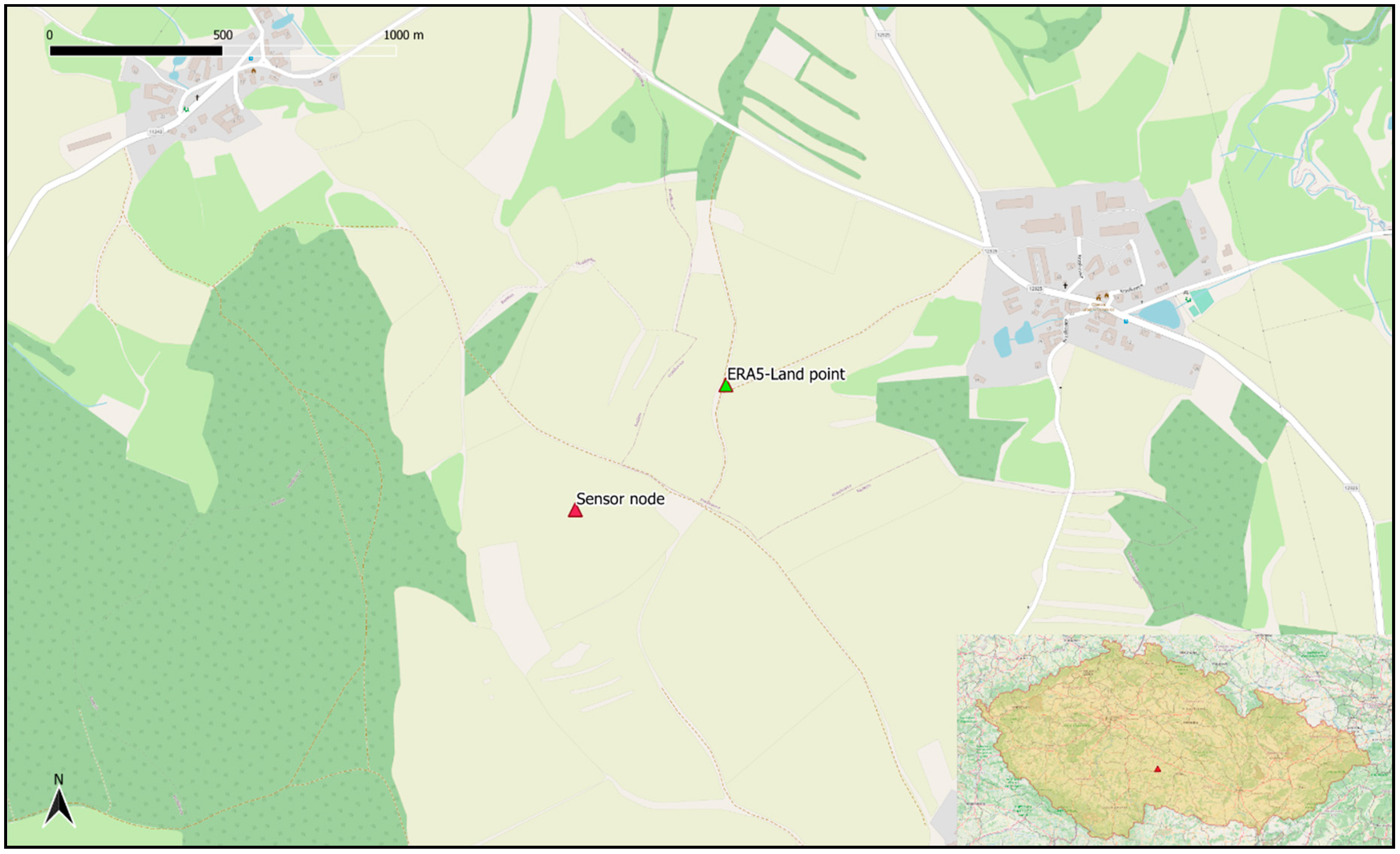
Observations used for the evaluation of global ERA5 data to compare physical variables were produced during the air and soil monitoring campaign in the year 2018 in the location of Kojčice village (15.22 E, 49.46 N) near Pelhřimov in the Czech Republic (see Figure 1). There was a set of sensor nodes deployed in the pilot locality in the fields. Most of the deployed nodes were equipped with sensors for soil monitoring, and one node was equipped with soil and air monitoring sensors. The air temperature in 2-m height above the ground was selected as the phenomena for comparing with the global ERA5-Land data set. The air temperature was measured by the combined multisensor VP-3 from the Decagon(R) Devices company. This sensor was measuring air temperature, humidity, and vapor pressure every 2 h from 21 March 2018 to 29 December 2018. Specifications of the used VP-3 multisensor for air temperature phenomenon are resolution 0.1 °C, range from −40 °C to +80 °C, and accuracy is defined by the continuous function where the maximum error is the function of the temperature. The maximum error for the measured range in the pilot locality is ±0.75 °C, but for most observations is ±0.5 °C and less. The distance between the sensor node position and the ERA5-Land reference point is approximately 350 m.

3.1.4. Case Study Area in the Pilsen Region

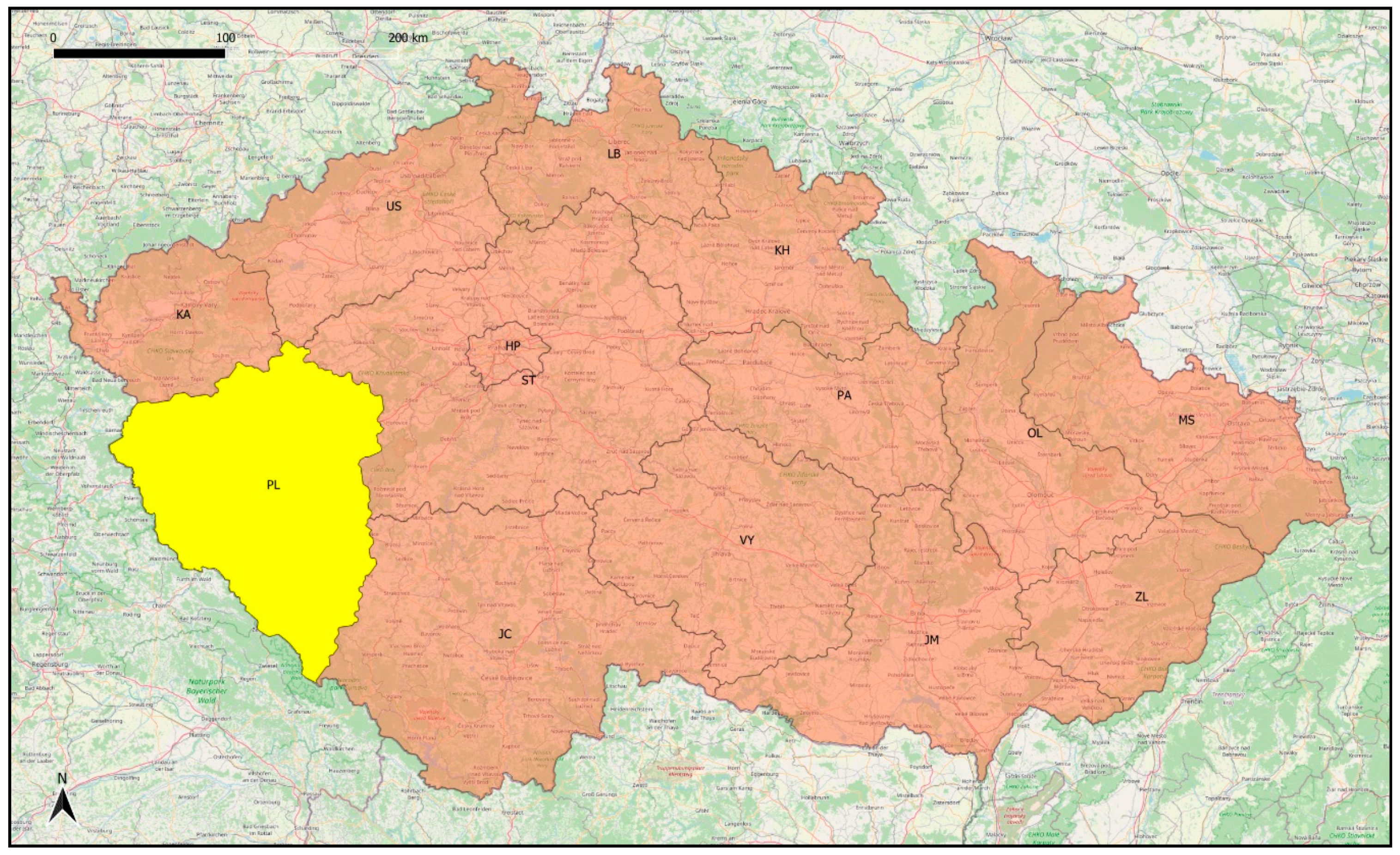
The Pilsen region (location of such a region is shown in Figure 2) was chosen as a case study for calculation of all agro-climatic factors mentioned in Section 3.2 because this area of interest is being investigated in various research projects supporting this contribution (see part Funding stated after Section 6. Conclusions).

It is worth stressing, even though the area of interest was chosen, the calculation of agro-climatic factors using hourly ERA5-Land data can be done for almost any particular place or area on the Earth, where the coverage of such a dataset is provided. Furthermore, thanks to the interactivity of scripts created, they have an area or place of interest as an input parameter. Methods, which are implemented for the area of interest, while respective outputs are provided here for each of such factors in basically two forms. In the form of graphs representing time-dependent manners of the particular factor for a specific place in the area of interest (geographical center of the Pilsen region) and the form of maps of such a region enable to see a spatial (or spatial-temporal) distribution of the calculated factor in the area. Examples of such maps are placed in Appendix A, whereby all the maps and graphs created for this area are available in [29]. The web page on GitHub was created to keep all of the Supplementary Materials in one place.

3.2. Methods

This section describes methods designed and developed for the calculation of certain agro-climatic factors. As a description of each method used is quite extensive, there is the first method described in full detail, and the rest of the method is outlined, stressing the critical parts of the process described by a flowchart of a particular method. In contrast, the comprehensive description of all the methods, together with the developed source code, is available as Supplementary Materials at https://github.com/JiriVales/agroclimatic-factors/wiki [29]. It is also worth mentioning that the algorithms are deployed at the https://test.euxdat.eu/ (The platform is being migrated to https://platform.euxdat.eu/) [30]—a cloud platform allowing the calculation of the particular agro-climatic factors on demand (for registered users only).

3.2.1. Frost-Free Periods

The agricultural season is primarily determined by the period of suitable temperatures for growing crops. Frost has a devastating effect on crops. In light frost (between 0 °C and −1/−2 °C), the tender plants are killed. Moderate freeze (between −2 °C and −4 °C) is widely destructive to most vegetation, and lower frost is already causing severe damage to most plants [31,32]. It is just a general simplification; the effects also vary for different growth stages (see [32] for details) and different crops. Therefore, farmers need to know the frost-free period in their agricultural areas. Significantly, the last spring frost date for starting agricultural work and the first fall frost date for the cessation of agricultural activities. The likelihood of frost and frost trends over the years helps effective fieldwork planning.

The last spring date is usually called the last day during spring (more correctly from winter to summer) when the minimum daytime temperature is less than 0 °C. The first fall date is the first day in the second half of the year (during autumn) when the minimum temperature is below zero. Usually, this date is given with a 50% or 10% probability (statistically from several years) that it will freeze later (spring date) or sooner (fall date). For farmers, knowledge of days with a low probability of frost is necessary for farming planning and decision-making to avoid destructive effects, hence dates with a last/first frost with a low probability (e.g., 10%) are desirable. The frost-free period is then a period from the last spring frost to the first fall frost. It includes a period suitable for growing crops.

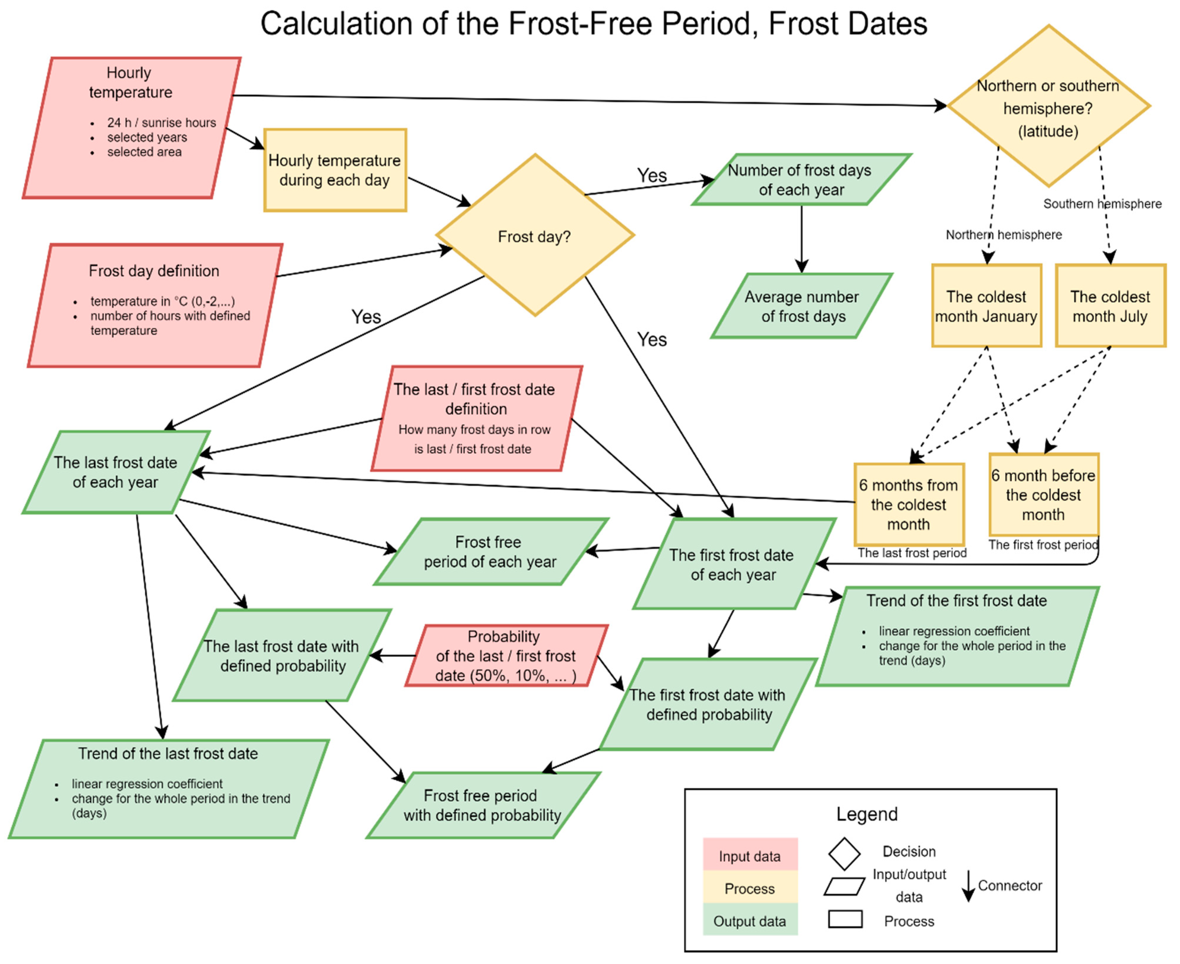
The minimum daily temperature is a necessary variable for determining frost dates. The daily minimum is determined as the lowest value of the hourly temperatures each day. We search for the days where the minimum is below 0 °C for at least one hour, see [33] for detailed justification. Subsequently, the algorithm calculates the last freezing day of each year for the spring period and the first freezing day for the autumn period. For the sake of simplicity, the coldest month is designated as January for the northern hemisphere and July for the southern hemisphere, which is the central month of the meteorologist winter season [34,35]. The hemisphere is determined from latitude. The resulting last spring frost date and first autumn frost date are calculated from the annual frost dates with a corresponding probability. The frost-free period is calculated as the period between the last and the first frost date. Similarly, it is possible to calculate the dates for another temperature threshold (e.g., for moderate freeze −2 °C).

By altering the input parameters, it is possible to calculate more days of frost in a row as the last/first frost date. The last/first frost date with defined probability is calculated from all selected years using the normal distribution, while the standard deviation and mean for the normal distribution is calculated from the frost dates of each year. Frost-free period with defined probability is calculated as the difference between these last and first frost dates. The flowchart of the designed algorithm is shown in Figure 3.

3.2.2. Crop Growth-Related Temperatures

There are four temperature thresholds, the cardinal temperatures, that define the relationship between temperature and crop growth. These thresholds are the absolute minimum, the optimum minimum, the optimum maximum, and the absolute maximum [10]. Based on such thresholds, the following three factors are defined and briefly described.

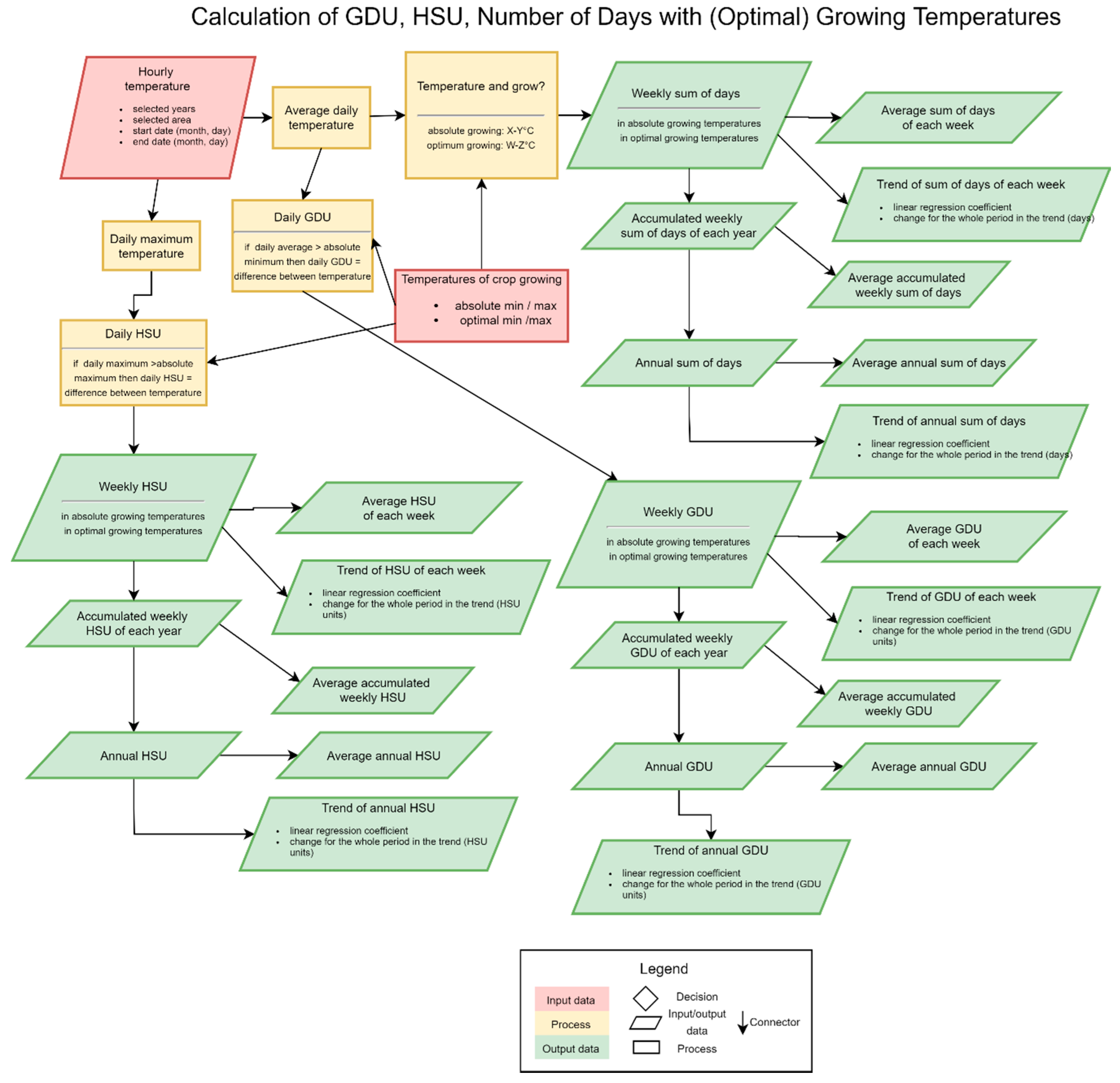
Heat stress units (HSU) are used to detect high temperatures unsuitable for crop growth. When the maximum daily temperature is higher than the absolute maximum temperature for crop growth, HSU is accumulated [10]. For example, if the threshold is exceeded by three degrees, three units are added.

Growing degree units (GDU) are used to relate temperature to crop development. GDU is accumulated when the average daily temperature exceeds the absolute minimum temperature threshold for the growth of a given crop. The difference between the daily temperature average and the temperature threshold of the plant is the accumulated GDU value for a given day [10]. For example, when the temperature is two degrees higher than the minimum for plant growth, two growing degree units are added.

The number of (optimal) growing days includes all growth days, days when the average temperature is in the interval from the absolute minimum to the absolute maximum of the selected crop. The number of days with optimal temperatures for growth is the sum of days when the average daily temperature is at the best temperatures for crop growth, between the optimal minimum and optimal maximum of the selected crop [10].

A flowchart of the designed algorithm for all three mentioned factors above is shown in Figure 4.

3.2.3. Uncertainty of Input Variables

Let us introduce how uncertainties of input variables for selected temperature-related agro-climatic factors (frost-free periods, growing degree units, heat stress units, number of (optimal) growing days, etc.) have been estimated. The data used for this section are described in the previous text, particularly in Section 3.1.1. ERA5-Land hourly data from 1981 to present and Section 3.1.2. ERA5 Ensemble of Data Assimilations.

To unify EDA and ERA5-Land data in the spatial domain, we decided to interpolate uncertainties for the test point in Kojčice, Czech Republic (see Section 3.1.3. Case study area in Kojčice for further information) from EDA by inverse distance method (defined by [36], with power parameter equal to 2). The computation of selected agro-climatic factors is mostly based on the daily averages of temperatures. Thus, the uncertainty of the daily temperature average has been calculated from interpolated values related to EDA. An exact formula was obtained by applying the error-propagation law to the average and has the following form:

$${\widehat{\sigma }}_D= \sqrt{\frac{{\sigma }_{T_1}^2+{\sigma }_{T_2}^2+\cdots +{\sigma }_{T_8}^2}{n}}$$

where D stands for the estimated uncertainty for a day D calculated from the interpolated values of temperature uncertainties ${\sigma }_{T_i}^2, i=1,2\dots 8,$ for the test point for each time i and n is equal to 8. The uncertainty of year temperature Y has been computed similarly to the uncertainty of day temperature. The exact formula is in the form:

$${\widehat{\sigma }}_Y=\sqrt{\frac{{\sigma }_{D_1}^2+{\sigma }_{D_2}^2+\cdots +{\sigma }_{D_{365\left(366\right)}}^2}{n}},$$

where n = 365 (366 for the leap year). The last two uncertainties dedicated to the temperature are uncertainties of daily maximum and minimum temperature denoted as ${\widehat{\sigma }}_{D_{max}}$ and ${\widehat{\sigma }}_{D_{min}}$, respectively. These have been computed by the following procedure. If the daily maximum and/or minimum temperature have been achieved at the same time as being in EDA, we took corresponding uncertainty from EDA. We remind readers that uncertainties in EDA are provided with the regular time step of three hours (please see 3.1.2). Otherwise, ${\widehat{\sigma }}_{D_{max}}$ and ${\widehat{\sigma }}_{D_{min}}$ have been interpolated by the linear interpolation from two uncertainties with neighboring hours in EDA.

3.2.4. Uncertainty of Calculated Agro-Climatic Factors

Uncertainties defined above allow us to calculate uncertainties of temperature-related agro-climatic factors, namely: (i) Annual number of frost days, (ii) annual number of days with growing temperatures, (iii) annual number of days with optimal growing temperatures, (iv) last spring frost date, (v) first fall frost date, (vi) frost-free periods, (vii) growing degree units, and (viii) heat stress units. In what follows, we will explain step by step how the uncertainty of all above mentioned temperature-related agro-climatic factors have been estimated.

We used the minimum temperature over a day and its uncertainty for the estimation of the uncertainty of (i) annual number of frost days, (iv) last spring frost date, and (v) first fall frost date. The uncertainty of (i) has been calculated as follows. Firstly, we calculated the number of frost days over a year as a summation of days in which the temperature was below 0 °C. Then uncertainties have been applied and we determined the maximum N_(f_max) and minimum number N_(f_min) of frost days by the following relation:

$$N_{f_{max}}={\sum }_i{D}_i, \mathrm{where} D_i=1 \mathrm{if} (D_{mi{n}_i}-{\widehat{\sigma }}_{D_{mi{n}_i}})\le 0 °\mathrm{C}, \mathrm{else} D_i= 0,$$

$$N_{f_{min}}={\sum }_i{D}_i, \mathrm{where} D_i=1 \mathrm{if} (D_{mi{n}_i}+{\widehat{\sigma }}_{D_{mi{n}_i}})\le 0 °\mathrm{C}, \mathrm{else} D_i= 0.$$

Note that the symbol $D_{mi{n}_i}$ represents the minimum temperature over an i-th day and ${\widehat{\sigma }}_{D_{mi{n}_i}}$ is its uncertainty. Finally, we set the confidence interval for the point estimator in the form ($N_{f_{min}},N_{f_{max}}$).

If $N_{f_{min}}>N_{f_{max}}$, the value $N_{f_{max}}$ has been replaced by $N_{f_{min}}$ in the confidence interval. Otherwise, i.e., if $N_{f_{min}}<N_{f_{max}}$, we substituted $N_{f_{min}}$ by $N_{f_{max}}$. The confidence interval for (iv) last spring frost date has been gained by the following procedure:

1. We found the latest date of the last spring frost date $L_{f_{max}}$ from the condition

$$(D_{mi{n}_i}-{\widehat{\sigma }}_{D_{mi{n}_i}})\le 0 °\mathrm{C}.$$

2. Then we identified the earliest date of the last spring frost date $L_{f_{min}}$ from the condition

$$(D_{mi{n}_i}+{\widehat{\sigma }}_{D_{mi{n}_i}})\le 0 °\mathrm{C}.$$

3. We put the values $L_{f_{min}}$ and $L_{f_{max}}$ into the confidence interval ($L_{f_{min}},L_{f_{max}}$).

The uncertainty of (v) first fall frost date has been estimated by applying the same procedure as for (iv). The only change is that we have been searching for the latest $F_{f_{max}}$ and earliest date $F_{f_{min}}$ of the first fall frost date and the confidence interval was then ($F_{f_{min}},F_{f_{max}}$). The agro-climatic factor, (vi) frost-free periods, is based on the frost days. Its uncertainty was estimated from the values of the earliest $L_{f_{min}}$ and latest $L_{f_{max}}$ date of the last spring frost date and the earliest $F_{f_{min}}$ and latest $F_{f_{max}}$ date of the first fall frost date. Uncertainties of frost-free period $F_{p_{min}}$ and $F_{p_{max}}$ have been calculated from:

$$F_{p_{min}}=F_{f_{min}}-L_{f_{max}} ,\hspace{1em}{F}_{p_{max}}=F_{f_{max}}-L_{f_{min}}.$$

The average temperature over an i-th day $D_{av{e}_i}$ and its uncertainty ${\widehat{\sigma }}_{D_{av{e}_i}}$ have been used for the determination of confidence intervals for (ii) annual number of days with growing temperatures, (iii) annual number of days with optimal growing temperatures, and (vii) growing degree units. The uncertainty of (ii) was obtained as:

Firstly, we calculated the minimal $N_{g_{min}}$ and the maximal $N_{g_{max}}$ number of growing days over a year as a summation of days as follows:

$$N_{g_{max}}={\sum }_i{D}_i, \mathrm{where} D_i=\{\begin{array}{c}{T}_{ab{s}_{min}}\le D_{av{e}_i}+{\widehat{\sigma }}_{D_{av{e}_i}}\\ T_{ab{s}_{max}}\ge D_{av{e}_i}-{\widehat{\sigma }}_{D_{av{e}_i}}\end{array},$$

$$N_{g_{min}}={\sum }_i{D}_i, \mathrm{where} D_i=\{\begin{array}{c}{T}_{ab{s}_{min}}\le D_{av{e}_i}-{\widehat{\sigma }}_{D_{av{e}_i}}\\ T_{ab{s}_{max}}\ge D_{av{e}_i}+{\widehat{\sigma }}_{D_{av{e}_i}}\end{array}.$$

Note that symbols $T_{ab{s}_{min}}$ and $T_{ab{s}_{max}}$ represent the minimum and maximum temperature for crop growing.

Secondly, we have values of $N_{g_{max}}$ and $N_{g_{min}}$ in our pocket so we can define the confidence interval ($N_{g_{min}},N_{g_{max}}$) for the annual number of days with growing temperatures.

The confidence interval of the annual number of days with optimal growing temperatures $N_{og}$ has been calculated by the above-mentioned approach. The only difference is the replacement of the minimum and maximum temperature for crop growing by the minimum and maximum temperature for optimal crop growing. The uncertainty of (vii) growing degree units was obtained by application of the following algorithm:

1. Calculation of minimal $D_{gd{u}_{min}}$ and maximal $D_{gd{u}_{min}}$ daily growing degree units as follows

$$D_{gd{u}_{max}}=\{\begin{array}{c}{D}_{av{e}_i}+{\widehat{\sigma }}_{D_{av{e}_i}}-T_{ab{s}_{min}} \mathrm{if} T_{ab{s}_{min}}< D_{av{e}_i}+{\widehat{\sigma }}_{D_{av{e}_i}} \\ D_{av{e}_i}+{\widehat{\sigma }}_{D_{av{e}_i}}-T_{ab{s}_{min}} \mathrm{if} T_{ab{s}_{max}} \ge D_{av{e}_i}-{\widehat{\sigma }}_{D_{av{e}_i}} \\ 0 \left(\mathrm{otherwise}\right)\end{array},$$

$$D_{gd{u}_{min}}=\{\begin{array}{c}{D}_{av{e}_i}-{\widehat{\sigma }}_{D_{av{e}_i}}-T_{ab{s}_{min}} \mathrm{if} T_{ab{s}_{min}}< D_{av{e}_i}-{\widehat{\sigma }}_{D_{av{e}_i}} \\ D_{av{e}_i}+{\widehat{\sigma }}_{D_{av{e}_i}}-T_{ab{s}_{min}} \mathrm{if} T_{ab{s}_{max}} \ge D_{av{e}_i}+{\widehat{\sigma }}_{D_{av{e}_i}} \\ 0 \left(\mathrm{otherwise}\right)\end{array}.$$

2. To get confidence intervals for growing degree units over a year we calculated minimal $A_{gd{u}_{min}}$ and maximal $A_{gd{u}_{min}}$ daily growing degree units by summation of $D_{gd{u}_{max}}$ and $D_{gd{u}_{min}}$.

The maximum temperature $D_{ma{x}_i}$ and its uncertainty ${\widehat{\sigma }}_{D_{ma{x}_i}}$ has been applied for calculation of confidence interval for (viii) heat stress units. In the first step, we calculated maximal $D_{hs{u}_{max}}$ and minimal $D_{hs{u}_{min}}$ values of heat stress units from the following condition:

$$D_{hs{u}_{max}}=\{\begin{array}{c}{D}_{ma{x}_i}+{\widehat{\sigma }}_{D_{ma{x}_i}}-T_{ab{s}_{max}} \mathrm{if} T_{ab{s}_{min}}< D_{ma{x}_i}+{\widehat{\sigma }}_{D_{ma{x}_i}}\\ 0 \left(\mathrm{otherwise}\right)\end{array},$$

$$D_{hs{u}_{min}}=\{\begin{array}{c}{D}_{ma{x}_i}-{\widehat{\sigma }}_{D_{ma{x}_i}}-T_{ab{s}_{max}} \mathrm{if} T_{ab{s}_{min}}< D_{ma{x}_i}-{\widehat{\sigma }}_{D_{ma{x}_i}}\\ 0 \left(\mathrm{otherwise}\right)\end{array}.$$

The maximal $A_{hs{u}_{max}}$ and minimal $A_{hs{u}_{min}}$ values of heat stress units over a year has been obtained as follows:

$$A_{hs{u}_{max}}={\sum }_i{D}_{hs{u}_{ma{x}_i}} , A_{hs{u}_{min}}={\sum }_i{D}_{hs{u}_{mi{n}_i}}.$$

Finally, we got the confidence interval ($A_{hs{u}_{min}},A_{hs{u}_{max}}$).

4. Results

Firstly, the input climatic data uncertainty and accuracy needed to be evaluated. This evaluation was proceeded in the pilot locality near Kojčice village (see Section 3.1.3. Case study area in Kojčice for further information). The village lies in a similar climatic environment as the main area of interest (Pilsen region), and we were able to gain access to at least a year-long time series of climatic measurements—which turned to be a complicated task to gain the sensor data directly from the Pilsen region.

After the evaluation process, we calculated the agro-climatic factors mentioned in Section 3.2. Methods, using data described in Section 3.1.1. ERA5-Land hourly data from 1981 to present for the case study areas (see Section 3.1.3 and Section 3.1.4 for information about such areas).

4.1. Uncertainty of Input Temperatures

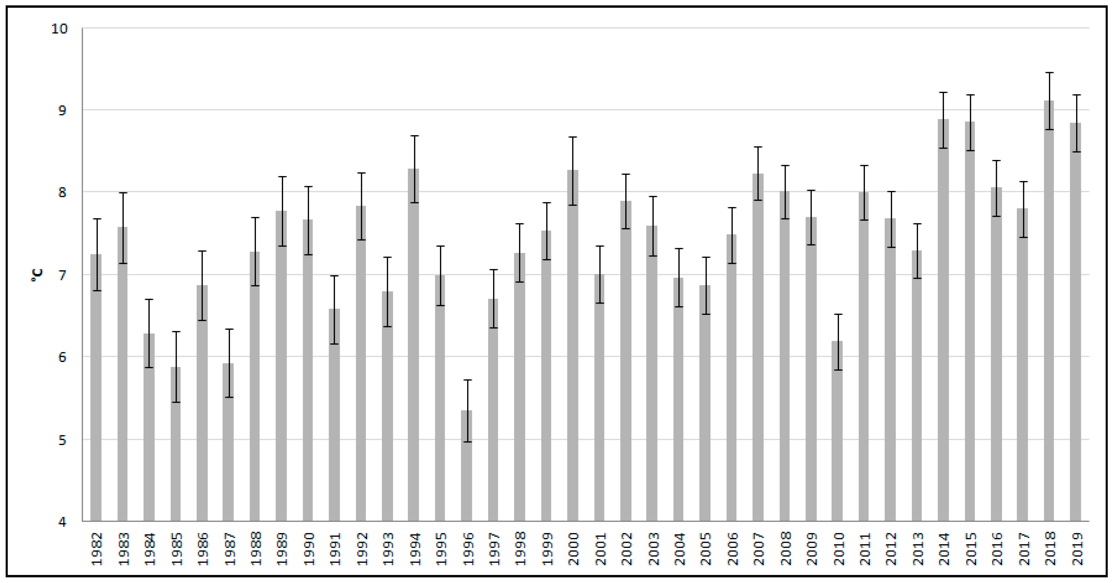
Firstly, the annual temperature uncertainties were calculated according to the first two formulas mentioned in Section 3.2.4, for the period 1982–2019 of the Kojčice area (depicted in Figure 5).

As can be seen from the graph in Figure 5, the annual temperature uncertainties provided by the EDA dataset are less than 0.5 °C, namely: min = 0.33 °C, max = 0.44 °C, a standard deviation of uncertainties is 0.3 °C. A table of particular values in the graph of Figure 5 is available in [29]. Similar tests can be run for other input data, using the same methodology.

4.2. Accuracy of the Global Climatic Data Evaluated Using In-Situ Sensors

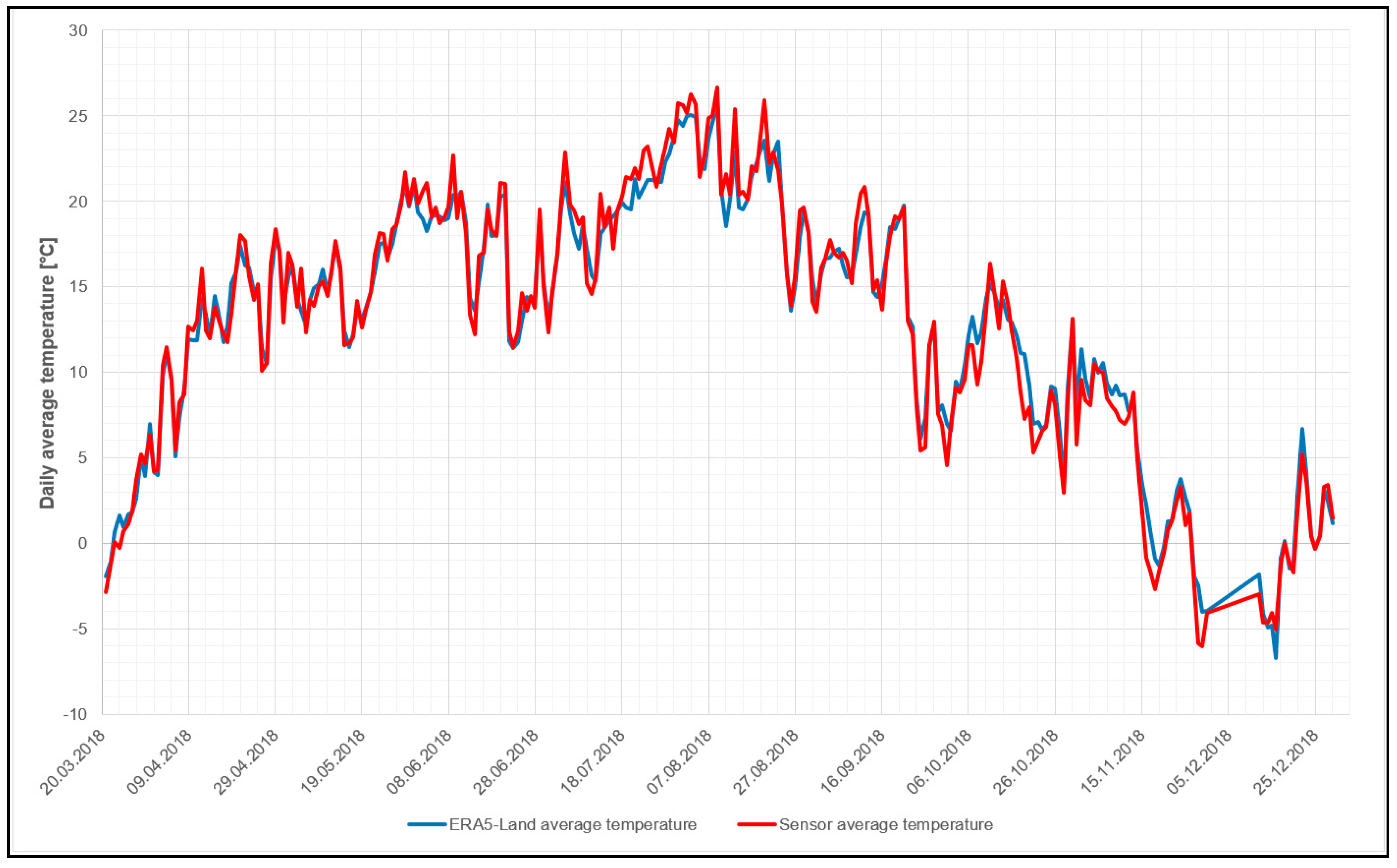
Next, the local in-situ sensor dataset was used for global model data accuracy evaluation. Comparison of values calculated from the model and values measured by the sensor directly in the field is useful for defining the reliability. Model data were provided hourly, while the sensor node was measuring every 2 h. Thus, the daily average temperature was selected as a value to be compared. A comparison of daily average temperatures calculated from ERA5-Land data and in-situ observations is depicted in Figure 6 below.

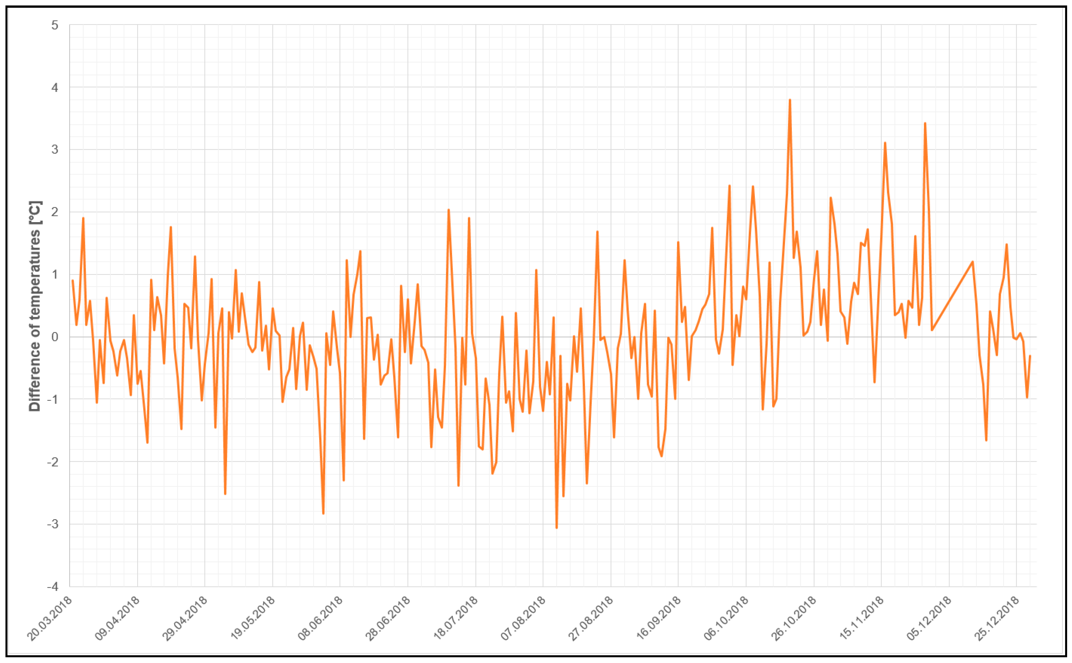
The difference chart depicted in Figure 7 clearly shows the differences between average daily temperatures calculated from ERA5-Land data and in-situ sensors during the period of observations. The differences are characterized by a standard deviation of 1.06 °C and min = −3.06 °C and max = 3.8 °C. Tables of particular values illustrated in Figure 5 and Figure 7 are available in [29].

The comparison of the temperatures gathered from global climatic data to in-situ sensor data, was possible to calculate from the limited period, but even that gives us a view of the reliability of the EDA dataset, describing the global data uncertainties. Results can be read in a way that the global data has (at least for our control measurements) approximately 3.5 times worse accuracy than the uncertainty described by the EDA (compare the 0.3 °C standard deviation of uncertainty to 1.06 °C standard deviation of the accuracy). Even with this disadvantage, the global data keep their value for the long time series provided. The relation of uncertainty and accuracy can (and will be) studied further, see discussion for details.

Also, it can be read from the above text and graphs, that the global temperature data oscillate around the temperatures measured by the in-situ sensor, which is here taken as a ground-truth for its inner accuracy of 0.1 °C. The oscillation is very problematic for frost-free period calculation, however the cumulative aspect of crop growth-related factors calculation (see Section 3.2.2) allows the use of global climatic data for the calculation of these factors (see also more in the discussion section).

4.3. Uncertainty of Calculated Agro-Climatic Factors

As the accuracy estimation needs the comparison to sensor data, it is not available, for the whole time series. Therefore, only the uncertainties of the input values were included in the calculation of the agro-climatic factors. As a result, we have the factors calculated together with information on the uncertainty of the calculation. All the factors were calculated for the whole available time series (years 1982–2019) and all the output graphs below portray the yearly values together with the uncertainty of the value.

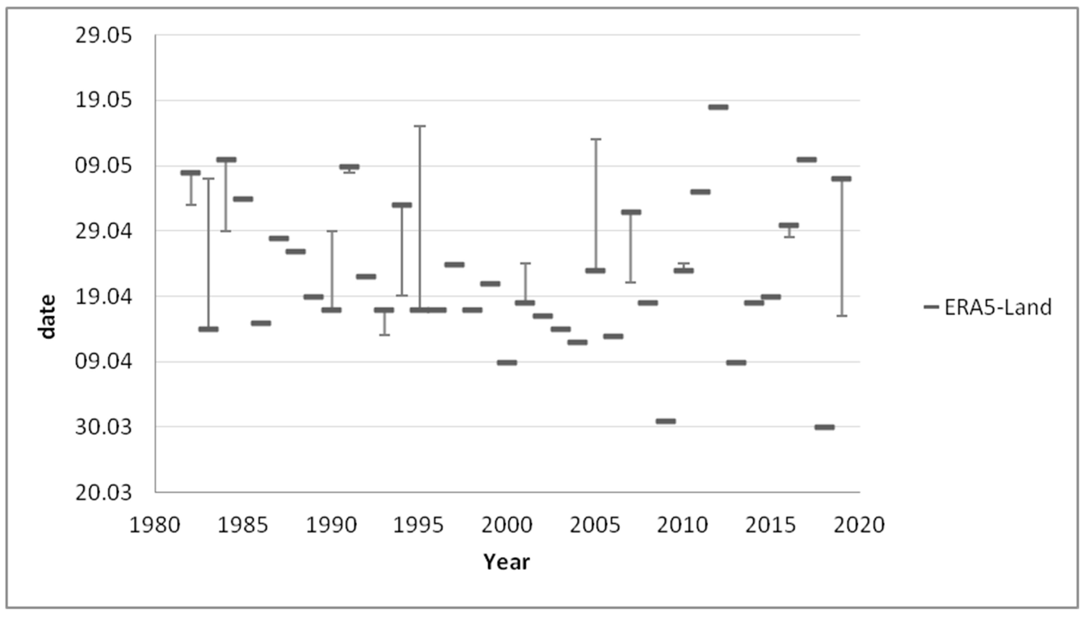
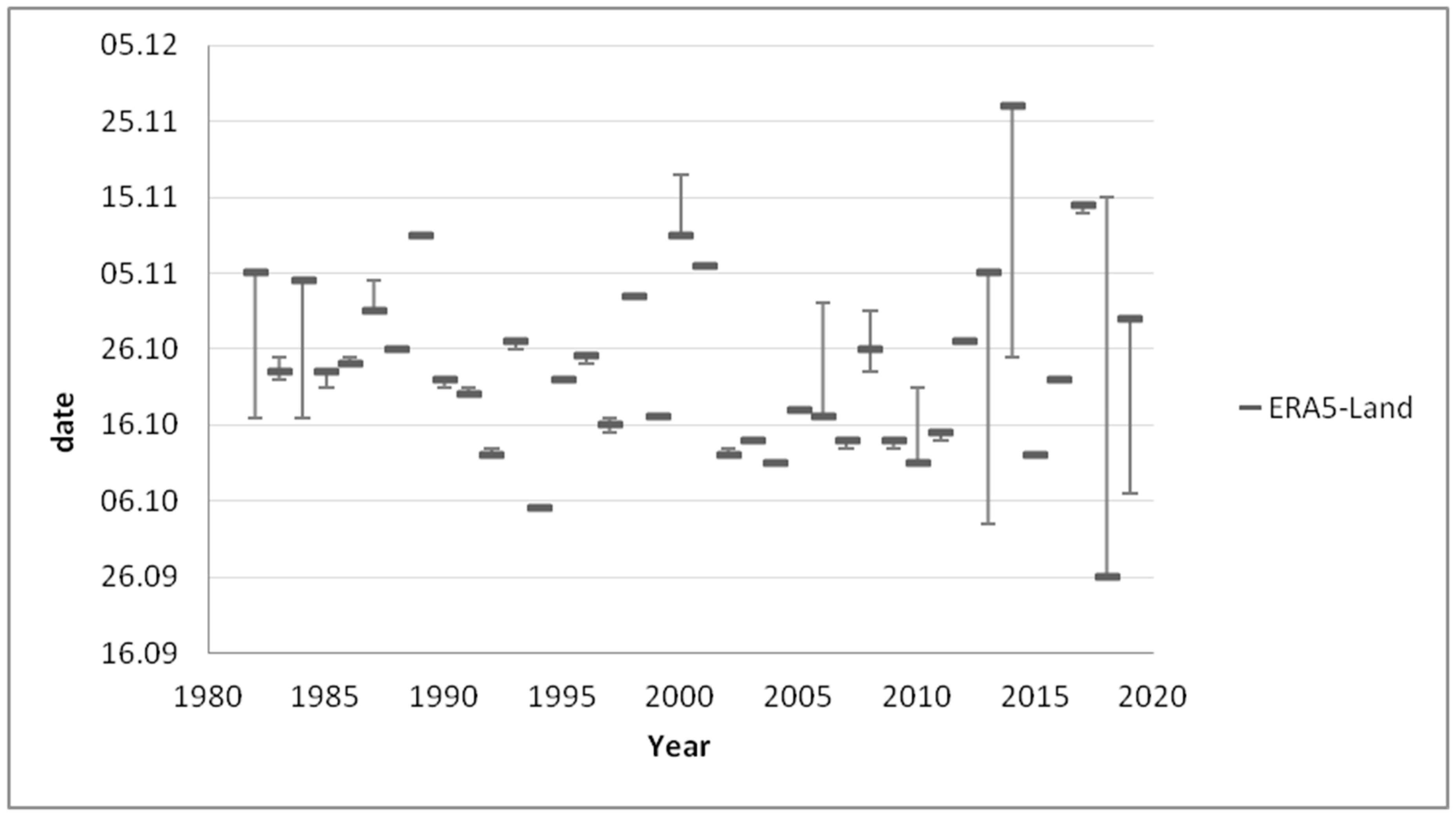
The first group of graphs relates to frost temperatures. Graphs of last spring and first fall frost dates are depicted in Figure 8 and Figure 9. The graph in Figure 10 shows the length of frost-free periods. Note that only if the uncertainty is large enough for the scale of the following graphs, it is visible.

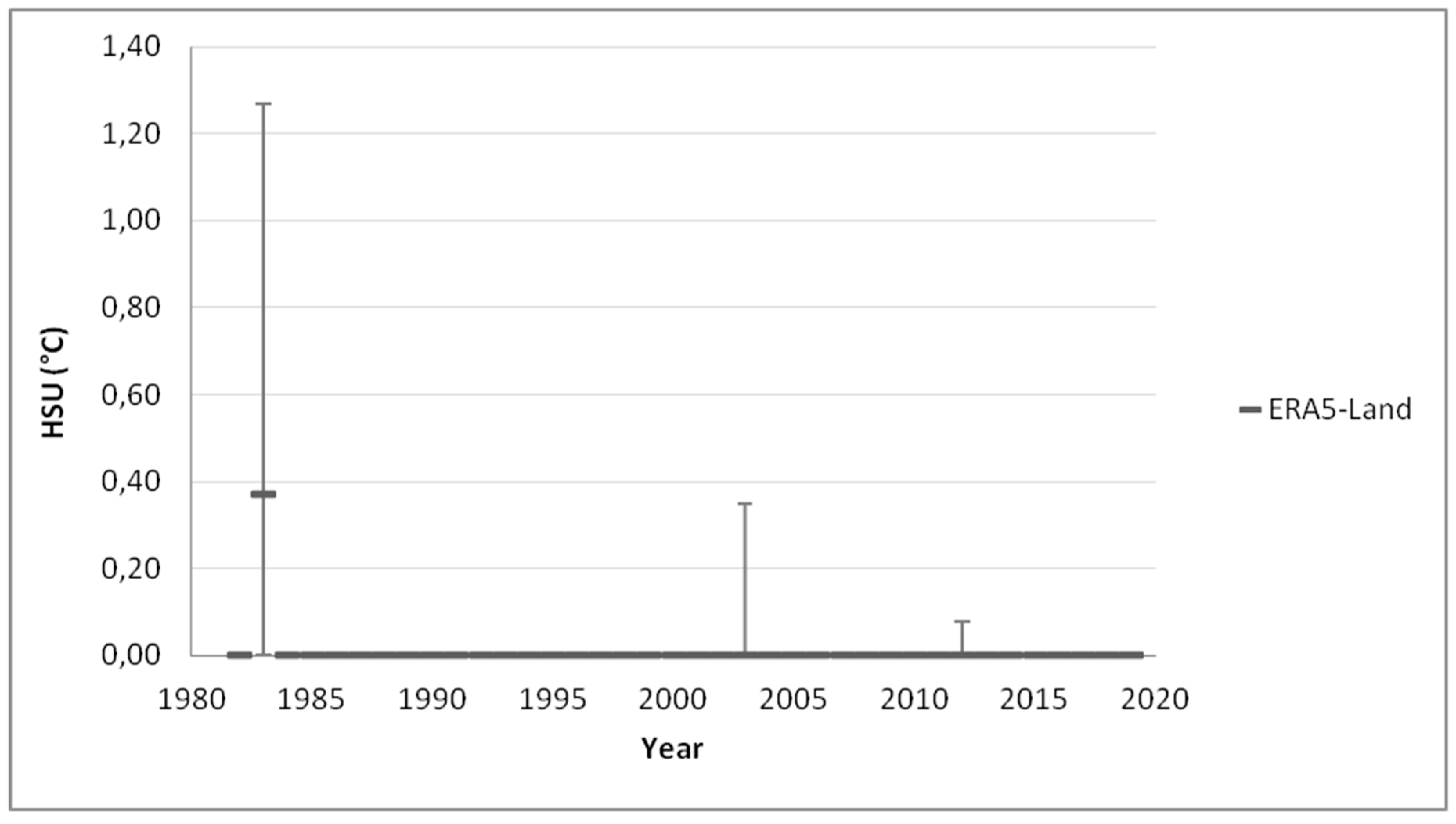
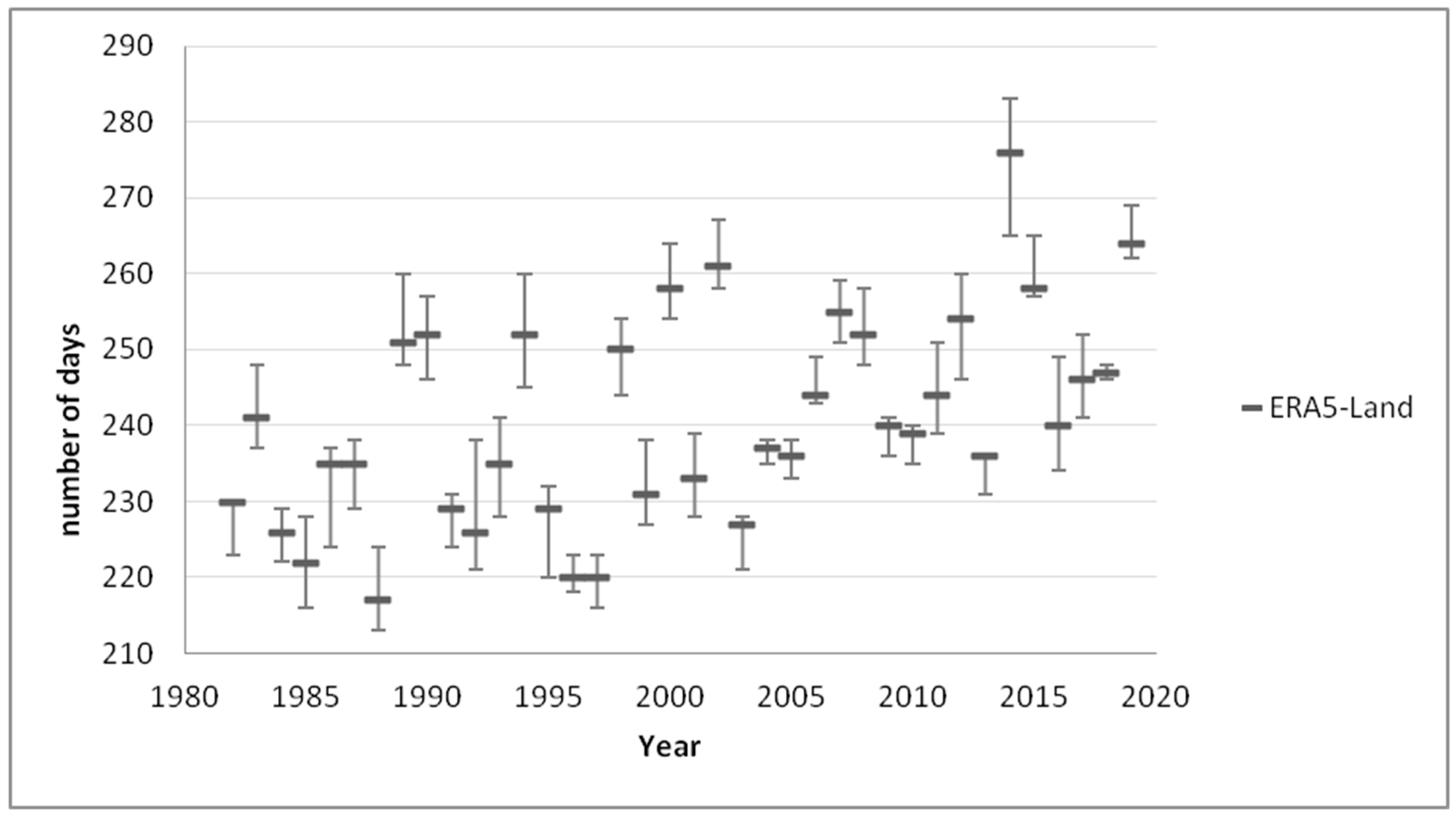
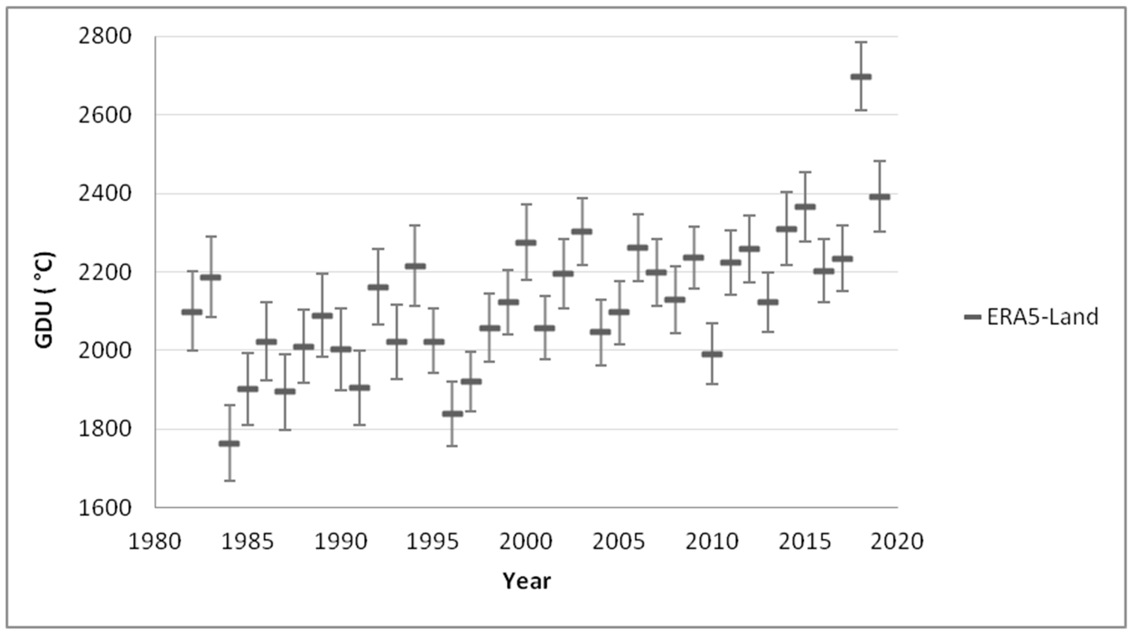
The next group of graphs is related to a particular crop type. The graphs portray the heat stress unit factor (Figure 11), growing degree unit factor (Figure 12), and the number of days with growing temperatures (Figure 13). These factors were calculated for C3 plants (such as wheat, soybean, and alfalfa) [10]. Crop temperature thresholds were therefore set as the average of a given group threshold range. The absolute minimum was set to 3.5 °C, the optimum minimum as 17.5 °C, the optimum maximum as 28 °C, and the absolute maximum to 32.5 °C. Please note that the heat stress occurs only exceptionally in the area of interest.

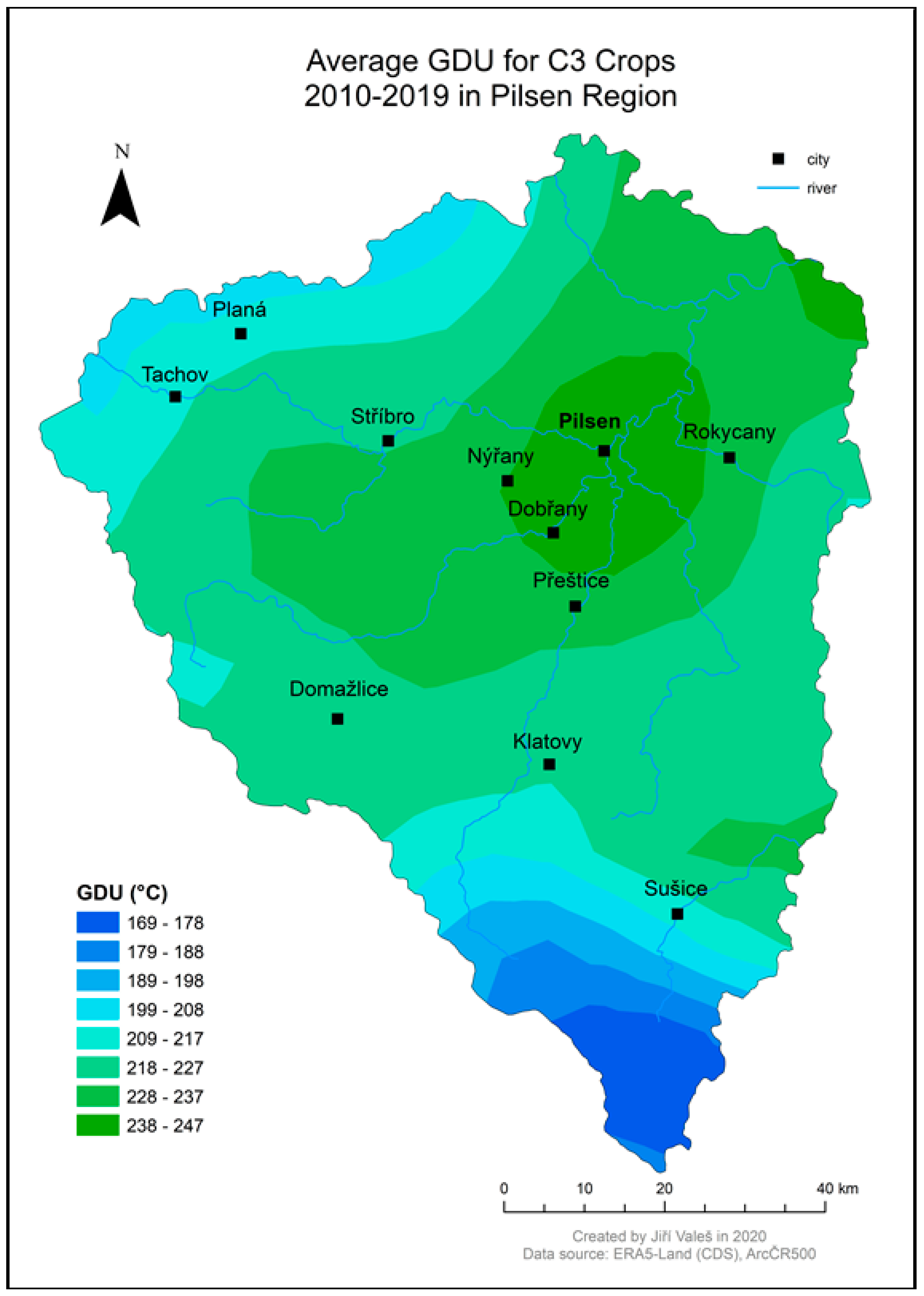
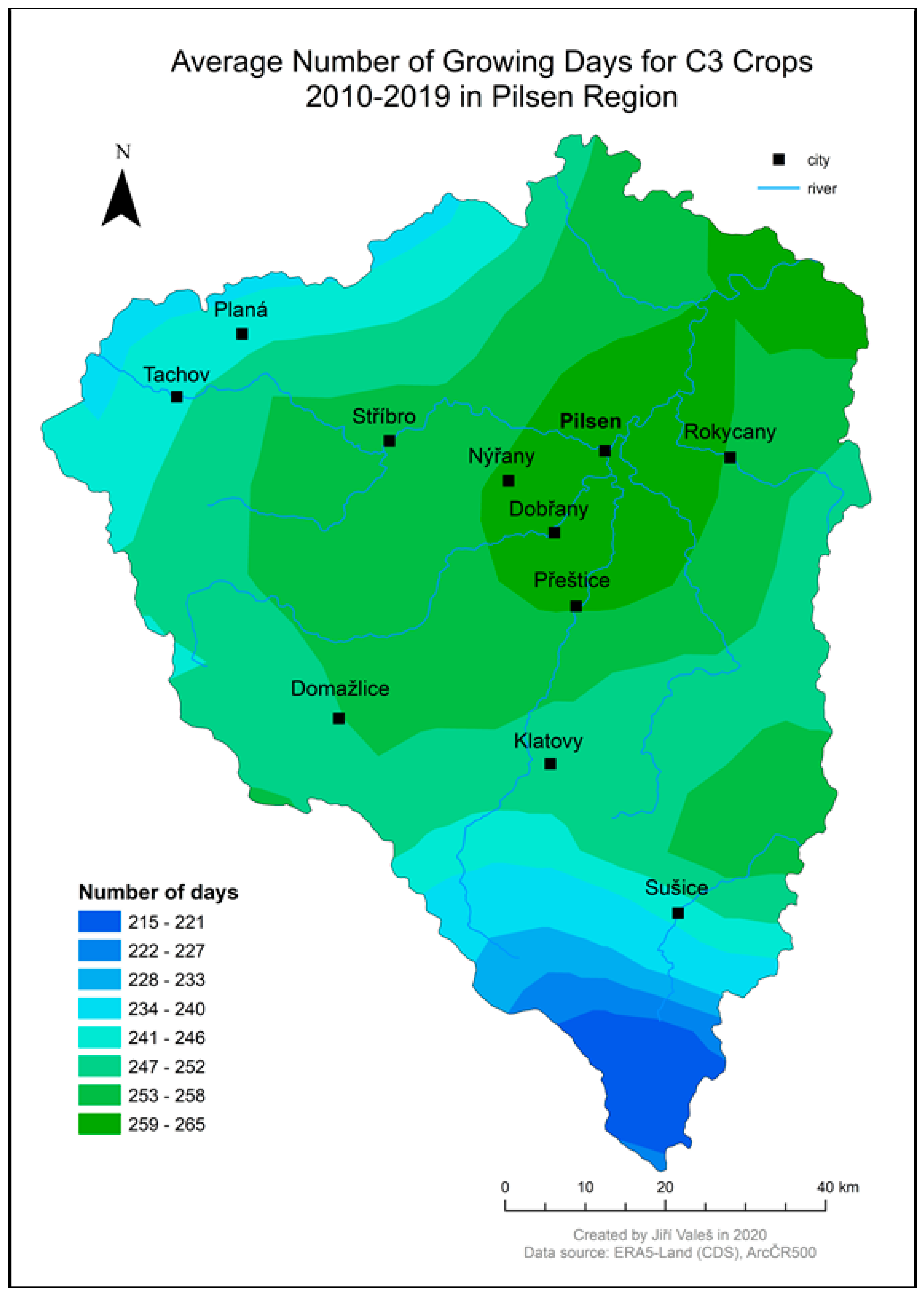
In order to demonstrate the spatial variability of the agro-climatic factors, two maps are attached as examples in Appendix A. The first map shows the average Growing Degree Units for C3 Crops 2010–2019 in the Pilsen Region (Figure A1). The second map shows the average Number of Growing Days for C3 Crops 2010–2019 in the Pilsen Region (Figure A2). A complete set of maps of agro-climatic factors created by the team are available in [29].

5. Findings and Discussion

The first significant output of this contribution lies in the evaluation of uncertainty and accuracy of the input climatic data. The example of temperature, as the climatic quantity, influencing the majority of agro-climatic factors, shows that even if the uncertainty in the data are pretty small (less than 0.5 °C for the whole period, with the standard deviation of 0.3 °C), the comparison to real in-situ measured data shows more significant differences (standard deviation of 1.06 °C and min = −3.06 °C and max = 3.8 °C). Such a difference urges caution in relying just on climatic data for calculation agro-climatic factors describing extremes (such as heat stress or frost dates). Still, the risks calculated from global data can be indicative, and a farmer naturally complements such information with a weather forecast.

The random character of the difference between climatic and sensor data ~ absence of a systematic shift (see graph in Figure 7) allows a farmer to rely on the temperature from climatic data for cumulative agro-climatic factors, such as the Number of growing (optimal) degree days or Number of (optimal) degree units.

Therefore, such results allow us to rely on the climatic data for calculation of at least temperature-dependent agro-climatic factors in the areas climatically similar to Kojčice (which is the area of the Pilsen region as well).

The algorithms were applied to the area of interest of the Pilsen region in the manuscript. However, they were also successfully deployed and tested in other areas during three hackathons: Climatic services for Africa (https://www.plan4all.eu/2019/04/team-2-progress-report-i/), leveraging of the algorithms by different teams in the San Juan hackathon (https://www.plan4all.eu/2019/10/san-juan-inspire-hackathon-2019/), and searching for Climate Change trends for Africa (https://www.plan4all.eu/2020/03/challenge-6-climate-change-trends-for-africa/).

Usage of the whole time series of the input data for calculation of the factors can document a local impact of climate change in a place of interest. For example, enlargement of the frost-free period in the Pilsen region can be interpreted from the time-dependent manners of last freezing and first freezing days graphs available in [29].

All the algorithms of agro-climatic factors calculation—designed, developed, and deployed in a cloud environment—can be widely re-used and evaluated by the scientific community, as they are available as open-source. It is also worth mentioning that the algorithms use the ERA5-Land dataset for now, but they can be easily applied to any other climatic data available.

There are limitations of visualization of big and multidimensional data—such as the agro-climatic factors calculated from the climatic data. Graphs perfectly describe the changes in a factor of time, but they are locked at one location. On the contrary, maps can describe the spatial distribution of a factor, but at one time, or its change during one period of time. As future work, the Space-Time Cube [37] principle can be leveraged for visualization of spatio-temporal aspects of a factor at once. Another limitation is related to the input data uncertainty and accuracy. As demonstrated in the manuscript, the input data uncertainty influences each agro-climatic factor differently. Therefore, we feel that it is crucial to work not only with the data values, but also the uncertainties in order to keep a final user of the algorithms informed.

We see several options to develop the work on this topic further. First, the rest of the agro-climatic factors (related to soil temperature, solar radiation, and water cycle) can also be calculated, including both input and output uncertainties. Moreover, we plan to compare the climatic data to more in-situ sensors in the future, once we gain access to such a data source, cooperation with the ISIDOR (http://www.emsbrno.cz/p.axd/en/Srážky.a.teploty.ISIDOR.html) network just started. It is also worth to mention, that Copernicus Climate Change Service continues in the reduction of the climatic data uncertainty, at least for Europe, see details in Copernicus regional reanalysis for Europe (CERRA) (https://climate.copernicus.eu/copernicus-regional-reanalysis-europe-cerra). Furthermore, last but not least, Copernicus Climate Change Service just announced that the ERA5 dataset has been reanalyzed and provides now time series going back to 1950.

6. Conclusions

The calculation of air temperature-related agro-climatic factors and their uncertainties from the open ERA5-Land dataset has been investigated within this manuscript. We designed algorithms for calculation of the most significant agro-climatic factors (frost-free period, heat stress units, growing degree units, number of growing days, dates of nitrogen application, water balance, and solar radiation), however only air temperature-related factors and their uncertainties (frost-free period, heat stress units, growing degree units, and number of growing days) have been elaborated further in the manuscript.

The developed algorithms were employed in numerical experiments. The first numerical experiment was validation of temperatures from the global ERA5-Land dataset on the in-situ sensor located in the area of Kojčice in Czechia. The direct comparison of temperature time series with the length of nine months showed an excellent fit between these two counterparts with a standard deviation better than 1.1 °C and with a correlation of 99%. This finding allowed us to estimate the frost-free period, heat stress units, growing degree units, and the number of growing days and their uncertainties in the Pilsen region from the ERA5-Land dataset over the period 1981–2019.

The conducted experiments showed that even global and relatively roughly distributed climate data are suitable for the calculation of agro-climatic factors on a regional scale with good accuracy. In addition, one could eventually use them if in-situ time series are not available or mix data from global models with terrestrial observations if time series are not long enough for agro-climatic factors calculation and analysis.

References

- Meteoblue. Meteoblue: History+. 2020. Available online: https://www.meteoblue.com/en/historyplus (accessed on 21 May 2020).
- National Oceanic and Atmospheric Administration (NOAA). When to Expect Your Last Spring Freeze. 2010. Available online: https://www.ncdc.noaa.gov/news/when-expect-your-last-spring-freeze (accessed on 21 May 2020).
- The Old Farmer’s Almanac. Yankee Publishing Inc. 2020. Available online: https://www.almanac.com/ (accessed on 21 May 2020).
- Ustrnul, Z.; Wypych, A.; Winkler, J.A.; Czekierda, D. Late spring freezes in Poland in relation to atmospheric circulation. Quaest. Geogr. 2014, 33, 165–172. [Google Scholar] [CrossRef] [Green Version]
- Index to Degree-Day Data and Maps of USA. 2009. Available online: http://pnwpest.org/US/ (accessed on 21 May 2020).
- Meteotemplate. Isle of Grain Weather. 2020. Available online: https://www.iogweather.org.uk/template/plugins/mapsUK/index.php (accessed on 21 May 2020).
- Environmental Indicators: Growing Degree Days. 2017. Available online: http://archive.stats.govt.nz/browse_for_stats/environment/environmental-reporting-series/environmental-indicators/Home/Atmosphere-and-climate/growing-degree-days.aspx (accessed on 21 May 2020).
- The Geography of Transport Systems: Length of Growing Period (LGP), in Days. 2010. Available online: https://transportgeography.org/?page_id=12891 (accessed on 21 May 2020).
- UNEP Environmental Data Explorer—The Environmental Database (Search | Map | Graph | Download). 2006. Available online: http://geodata.grid.unep.ch/ (accessed on 21 May 2020).
- Hollinger, S.E.; Angel, J.R. Illinois Agronomy Handbook: Weather and Crops. 2012. Available online: http://extension.cropsciences.illinois.edu/handbook/pdfs/chapter01.pdf (accessed on 21 May 2020).
- Pathak, T.; Hubbard, K.; Shulski, M. Soil Temperature: A Guide for Planting Agronomic and Horticulture Crops in Nebraska; University of Nebraska: Lincoln, NE, USA, 2012. [Google Scholar]
- SolarGIS. Global Solar Atlas. 2020. Available online: https://globalsolaratlas.info/map (accessed on 21 May 2020).
- Giusti, M. ERA5: Dataset Documentation. 2019. Available online: https://confluence.ecmwf.int/display/CKB/ERA5 (accessed on 21 May 2020).
- Afonin, A.N.; Greene, S.L.; Dzyubenko, N.I.; Frolov, A.N. (Eds.) Interactive Agricultural Ecological Atlas of Russia and Neighboring Countries. Economic Plants and their Diseases, Pests and Weeds. 2008. Available online: http://www.agroatlas.ru (accessed on 21 May 2020).
- Bishop, J.K.B.; Rossow, W.B.; Dutton, E.G. Surface solar irradiance from the International Satellite Cloud Climatology Project 1983–1991. J. Geophys. Res. 1997, 102, 6883–6910. [Google Scholar] [CrossRef]
- Markovic, S.; Luka, B.; Cerekovic, N.; Kljajić, N.; Rudan, N. Rainfall Analyses and Water Deficit during Growing Season in Banja Luka Region. Int. Congr. Ecol. Ecol. Spectr. 2012, 4167, 1167–1176. [Google Scholar]
- Geography, A.L. The Water Balance. 2016. Available online: https://www.alevelgeography.com/water-balance/ (accessed on 21 May 2020).
- El Dorado Weather: Australia Yearly Rainfall Averages. 2010. Available online: https://www.eldoradoweather.com/forecast/australia/australia-yearly-rainfall.html (accessed on 21 May 2020).
- Canada.ca: Agroclimatic Atlas of Canada. 1976. Available online: http://sis.agr.gc.ca/cansis/publications/manuals/1976-acac/index.html (accessed on 21 May 2020).
- Globální Klimatické Modely | Klimatická Změna v České Republice. 2020. Available online: https://www.klimatickazmena.cz/cs/metodika/globalni-klimaticke-modely/ (accessed on 21 May 2020). (In Czech).
- Adisa, O.M.; Botai, C.M.; Botai, J.O.; Hassen, A.; Darkey, D.; Tesfamariam, E.; Adisa, A.F.; Adeola, A.M.; Ncongwane, K.P. Analysis of agro-climatic parameters and their influence on maize production in South Africa. Theor. Appl. Climatol. 2018, 134, 991–1004. [Google Scholar] [CrossRef]
- Trnka, M.; Olesen, J.E.; Kersebaum, K.C.; Skjelvåg, A.O.; Eitzinger, J.; Seguin, B.; Peltonen-Sainio, P.; Rötter, R.; Iglesias, A.; Orlandini, S.; et al. Agroclimatic conditions in Europe under climate change. Glob. Chang. Biol. 2011, 17, 2298–2318. [Google Scholar] [CrossRef] [Green Version]
- Copernicus Climate Change Service (C3S): C3S ERA5-Land Reanalysis. 2019. Available online: https://cds.climate.copernicus.eu/cdsapp#!/home (accessed on 19 May 2020).
- Yang, X. ERA5-Land: Data Documentation. 2020. Available online: https://confluence.ecmwf.int/display/CKB/ERA5-Land (accessed on 19 May 2020).
- European Centre for Medium-Range Weather Forecasts (ECMWF): ERA5-Land. 2020. Available online: https://www.ecmwf.int/en/era5-land (accessed on 19 May 2020).
- European Centre for Medium-Range Weather Forecasts (ECMWF): IFS Documentation CY45R1. 2018. Available online: https://www.ecmwf.int/en/elibrary/18714-part-iv-physical-processes (accessed on 19 May 2020).
- Hennermann, K. ERA5: Uncertainty Estimation. 2020. Available online: https://confluence.ecmwf.int/display/CKB/ERA5%3A+uncertainty+estimation (accessed on 19 May 2020).
- Isaksen, L.; Bonavita, M.; Buizza, R.; Fisher, M.; Haseler, J.; Leutbecher, M.; Raynaud, L. Ensemble of Data Assimilations at ECMWF; ECMWF: Reading, UK, 2010; Available online: https://www.ecmwf.int/en/elibrary/10125-ensemble-data-assimilations-ecmwf (accessed on 19 May 2020). [CrossRef]
- Valeš, J. JiriVales/Agroclimatic-Factors: Algorithms of Creation Agroclimatic Factors from Climatic Dataset ERA5-Land (Necdf Files), GitHub, Inc. 2020. Available online: https://github.com/JiriVales/agroclimatic-factors/wiki (accessed on 21 May 2020).
- E-Infrastructure of the Project European e-Infrastructure for Extreme Data Analytics in Sustainable Development (EUXDAT). 2020. Available online: https://test.euxdat.eu/ (accessed on 21 May 2020).
- Geslin, H.; Holzberg, I.A.; Mason, B. Protection against Frost Damage (Report of a Working Group of the Commission for Agricultural Meteorology), World Meteorological Organization (WMO). 1963. Available online: https://library.wmo.int/index.php?lvl=notice_display&id=5363#.XyKxBCgzaUl (accessed on 21 May 2020).
- Shroyer, J.P.; Mikesell, M.E.; Paulsen, G.M. Spring Freeze Injury to Kansas Wheat. Cooperative Extension Service, Kansas State University. 1995. Available online: https://bookstore.ksre.ksu.edu/pubs/C646.pdf (accessed on 13 August 2020).
- Ahrens, C.D. Meteorology Today, 8th ed.; Brooks/Cole Publishing: Belmont, CA, USA, 2006; ISBN 0-49501162-2. [Google Scholar]
- Haby, J. Which Months of the Year Are Typically Coldest? 2004. Available online: https://www.theweatherprediction.com/habyhints3/980/ (accessed on 19 May 2020).
- National Centers for Environmental Information (NCEI). Meteorological Versus Astronomical Seasons. 2016. Available online: https://www.ncei.noaa.gov/news/meteorological-versus-astronomical-seasons (accessed on 19 May 2020).
- Shepard, D. A two-dimensional interpolation function for irregularly-spaced data. In Proceedings of the 1968 ACM National Conference, New York, NY, USA, 27–29 August 1968; pp. 517–524. [Google Scholar] [CrossRef]
- Kraak, M.J.; Koussoulakou, A. A Visualization Environment for the Space-Time-Cube. In Developments in Spatial Data Handling; Springer: Berlin/Heidelberg, Germany, 2005. [Google Scholar] [CrossRef]
Figure 1.
Location of the sensor node, and reference point for ERA5-Land model, location of the locality in the Czech Republic (overview map).
Figure 2.
Regions of the Czech Republic with the highlighted Pilsen region in yellow.
Figure 3.
Scheme of the algorithm for calculation frost dates and frost-free period (adapted from [29]).
Figure 4.
Scheme of the algorithm for calculation of growing degree units (GDU), heat stress units (HSU), and the number of growing days (adapted from [29]).
Figure 5.
Graph of average annual temperature with Ensemble Data Assimilations (EDA) uncertainties during the years 1982–2019 in the Kojčice area.
Figure 6.
Graph of daily average temperatures calculated from ERA5-Land data (blue line), in-situ observations (red line). The Pearson correlation coefficient is equal to 0.99.
Figure 7.
Graph showing the differences between ERA5-Land data and in-situ observations.
Figure 8.
Graph of last spring frost dates with uncertainties between the years 1982 and 2019.
Figure 9.
Graph of first fall frost dates with uncertainties between the years 1982 and 2019.
Figure 10.
Graph of frost-free periods with uncertainties between the years 1982 and 2019.
Figure 11.
Graph of annual HSU for C3 crops between the years 1982 and 2019.
Figure 12.
Graph of the number of days with growing temperatures for C3 crops with uncertainties between the years 1982 and 2019.
Figure 13.
Graph of annual GDU for C3 crops between the years 1982 and 2019.
Publisher’s Note: MDPI stays neutral with regard to jurisdictional claims in published maps and institutional affiliations. |
© 2021 by the authors. Licensee MDPI, Basel, Switzerland. This article is an open access article distributed under the terms and conditions of the Creative Commons Attribution (CC BY) license (http://creativecommons.org/licenses/by/4.0/).
Share and Cite
MDPI and ACS Style
Jedlička, K.; Valeš, J.; Hájek, P.; Kepka, M.; Pitoňák, M. Calculation of Agro-Climatic Factors from Global Climatic Data. Appl. Sci. 2021, 11, 1245. https://0-doi-org.brum.beds.ac.uk/10.3390/app11031245
AMA Style
Jedlička K, Valeš J, Hájek P, Kepka M, Pitoňák M. Calculation of Agro-Climatic Factors from Global Climatic Data. Applied Sciences. 2021; 11(3):1245. https://0-doi-org.brum.beds.ac.uk/10.3390/app11031245
Chicago/Turabian StyleJedlička, Karel, Jiří Valeš, Pavel Hájek, Michal Kepka, and Martin Pitoňák. 2021. "Calculation of Agro-Climatic Factors from Global Climatic Data" Applied Sciences 11, no. 3: 1245. https://0-doi-org.brum.beds.ac.uk/10.3390/app11031245
Note that from the first issue of 2016, this journal uses article numbers instead of page numbers. See further details here.