Classification of Plant Electrophysiology Signals for Detection of Spider Mites Infestation in Tomatoes

Abstract

Herbivorous arthropods, such as spider mites, are one of the major causes of annual crop losses. They are usually hard to spot before a severe infestation takes place. When feeding, these insects cause external perturbation that triggers changes in the underlying physiological process of a plant, which are expressed by a generation of distinct variations of electrical potential. Therefore, plant electrophysiology data portray information of the plant state. Analyses involving machine learning techniques applied to plant electrical response triggered by spider mite infestation have not been previously reported. This study investigates plant electrophysiological signals recorded from 12 commercial tomatoes plants contaminated with spider mites and proposes a workflow based on Gradient Boosted Tree algorithm for an automated differentiation of the plant’s normal state from the stressed state caused by infestation. The classification model built using the signal samples recorded during daylight and employing a reduced feature subset performs with an accuracy of 80% in identifying the plant’s stressed state. Furthermore, the Hjorth complexity encloses the most relevant information for discrimination of the plant status. The obtained findings open novel access towards automated detection of insect infestation in greenhouse crops and, consequently, more optimal prevention and treatment approaches.

1. Introduction

Each year, approximately one-fourth of the agricultural production is damaged by herbivorous arthropods, such as spider mites [1,2]. Spider mites represent the most important family of mites with the ability to feed on many host plants [3,4], but they are very hard to detect before severe contamination occurs. Early and automated detection of spider mites attacks would prevent crop losses and result in more effective crop protection. Additionally, it would allow optimal use of pesticides leading to lower environmental impacts from agriculture [5].

As living organisms, plants possess a defense mechanism that helps them react to both biotic and abiotic environmental stresses, at either molecular, physiological or morphological level [6,7,8]. A single perturbation triggers changes in the underlying physiological process of a plant, which are expressed by distinct variations in the electrical potential [9]. Hence, the emitted bioelectrical signal portrays the changes in a plant’s state and, therefore, exhibits strong potential for quick detection of the cause of the state change.

Although sparse, current literature asserts automated recognition of signal pattern changes in the plant electrophysiological response induced by different stressors. Either by inspecting local features or by analyzing the shape of the entire recorded waveform, the proposed approaches, which employ binary classification algorithms, provide accurate identification of the plant stressed state caused by the applied stimuli [10,11,12,13,14,15].

The major parts of the analyzed stimuli are abiotic stressors, such as the environmental stressors of light, cold and osmotic stress [10]; the pollution stressors sodium chloride, sulphuric acid and ozone [11,12]; drought [15]; as well as salt tolerance [13], applied either on soybeans, tomato, cucumber, cabbage or wheat. However, the analyses for identifying electrophysiological alteration caused by a biotic stress at whole-plant level emerged only with a very recent study investigating the electrical signaling response of tomato plants to a pathogenic fungus [14]. Otherwise, most of the studies on crop focused on wounding caused by herbivory inducing long electrical signaling [16,17,18].

With the exception of [15], all of the proposed approaches explored data acquired within controlled laboratory settings and inside a Faraday cage, which limits their application in the typical production environment. Moreover, to the best of our knowledge, the plant electrophysiology response has not yet been analyzed for potential detection of eventual changes in the signal patterns caused by the presence of infestation with spider mites.

The findings presented in [15] demonstrate continuous and stable long-term recordings of plant electrophysiology signals in regular greenhouse conditions (i.e., outside of a Faraday cage) with the newly developed sensor PhytlSigns (Vivent SA, Crans-près-Celigny, Switzerland). Such findings allow access to direct crop monitoring and potentially automated real-time assessment of a plant’s state in standard growing environments. Furthermore, it was also shown that electrical potential variations follow nycthemeral rhythm (i.e., basal level during the night with higher values during the daylight), which is potentially related to photosynthesis. Hence, considering their metabolism, the plants could react differently to an infestation in different periods of the day.

The aim of this study is to explore electrophysiology signals acquired with PhytlSigns from commercial tomato plants growing in a typical production environment during a spider mite infestation. More precisely, it employs signal processing and supervised machine learning techniques to assess the possibility to automatically distinguish eventual pattern changes in the electrical plant response related to the plant stress induced by the presence of spider mites. Additionally, to assess eventual differences in the plant response, data analysis was also performed on separated datasets, including (i) signals recorded during daylight and (ii) signals recorded during the night. Moreover, to address the lack of reported findings in this domain, this study also explores a relatively broad range of signal features to discern those with more discriminative power for identifying plant stress.

2. Materials and Methods

2.1. Study Design

Tetranychus urticae were reared on tomato plants (Solanum lycopersicum L. cv. Admiro), in cages made of a fine nylon mesh (mesh diameter = 250 μm). All cages were kept in a climate chamber at 70 ± 10% r.h., 24 ± 2 °C/22 ± 2 °C, and 16 h light/8 h dark photo period. The rearing was carried out at Hepia Lullier (Switzerland). The colonies of T. urticae were initiated more than 3 months before the beginning of the experiment [19].

The experiment was conducted from late August until mid-September at the field station of Agroscope Conthey (Switzerland) in a 90 m² glasshouse equipped with lateral and roof ventilations, fogging and shading for climate regulation. The greenhouse was divided into 16 experimental cages (L × W × H = 1.75 × 1.75 × 2.5 m) in a Latin square split-plot design with four cages × four treatments: control, T. urticae + treatment 1, T. urticae + treatment 2, T. urticae + treatment 3. To prevent potential sources of arthropod escape, each cage was enclosed in a fine nylon mesh (diameter = 250 μm) on all sides. Access to the plants was possible through a small zipped opening with additional Velcro^® closings on two edges. Cages were separated by a distance of approximately 0.40 m. In each cage, three 50-day-old tomato plants, crop variety Admiro, were placed about 0.70 m from each other. Plants were grown in 10 L pots in a substrate of 1/3 black peat and 2/3 Ricoter^® mix made of 65% blond peat, 15% sand, 20% perlite (Aarberg, Switzerland). A standard fertilizing solution for tomato plants was automatically provided by drip irrigation. A data logger (DGT-Volmatic sensor RTF-5D, Senmatic A/S, Denmark) in one cage recorded temperature and relative humidity throughout the experiments.

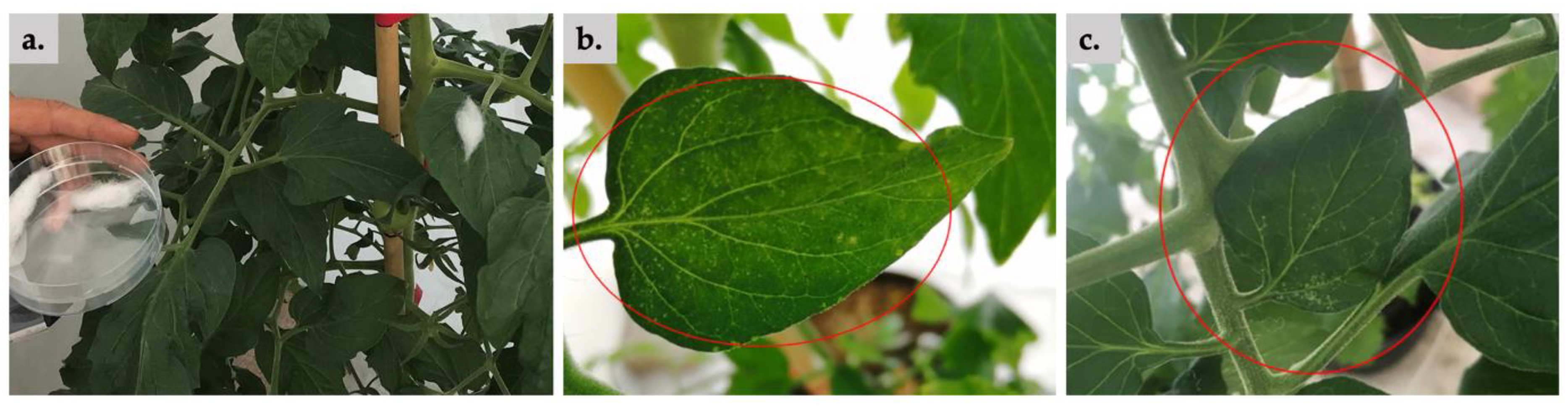
Except for the control set, each tomato plant was inoculated with 30 mobile stages (protonymphs and deutonymphs) of T. urticae, on “Day 0”. Mites were collected from the rearing units, counted under a magnifying lens and transferred with a thin paintbrush to a cotton pad as positioning support. The cotton was then attached to tomato leaves to allow the spider mites to colonize their host plant (panel a. in Figure 1). Fifteen days after infestation (“Day 15”), a phytosanitary treatment was applied to halt the plants’ infestation.

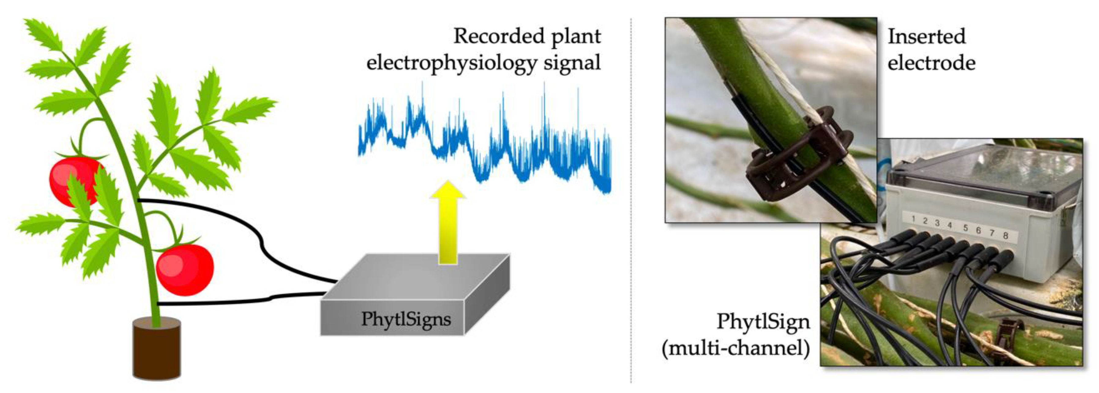
Throughout the experiment’s entire duration, recordings of electrophysiological signals of 32 plants (8 control and 24 infested plants) were done at 500 Hz sampling rate using four multi-channel PhytlSigns devices. This measuring device, which is designed with a very high input impedance, of the order of many MΩ, includes eight pairs of custom-built electrodes, each of them made of a 0.5 mm diameter silver-coated copper wire covered with a 2.79 mm diameter coaxial cable with impedance of 50 Ω [15]. The importance of impedance matching in plant electrophysiology measurements has been highlighted [20]. The pair of electrodes comprises one active and one ground (i.e., reference) electrode. The active electrodes were placed above the plant’s first floral bud, whereas the reference electrodes were placed below the first leaf. Figure 2 gives a schematic representation of the recordings’ setup.

To assure stability in the recorded signal, the electrodes need to be inserted in the conducting bundles of the plant [21]. Hence, the signal stability was monitored within the initial 72 h of the experiment during which the electrodes were repositioned when an unstable recording was observed.

The severity of the infestation was assessed by counting the number of spider mites remaining on each plant on the 3rd, 6th, 9th, 11th, and the 14th day after the contamination. Out of the 24 contaminated plants, 12 were assessed as strongly infested with spider mites; therefore, only the recorded data coming from these 12 plants were considered in the presented analysis. The visual appearance of the infested leaves is shown in Figure 1.

2.2. Data

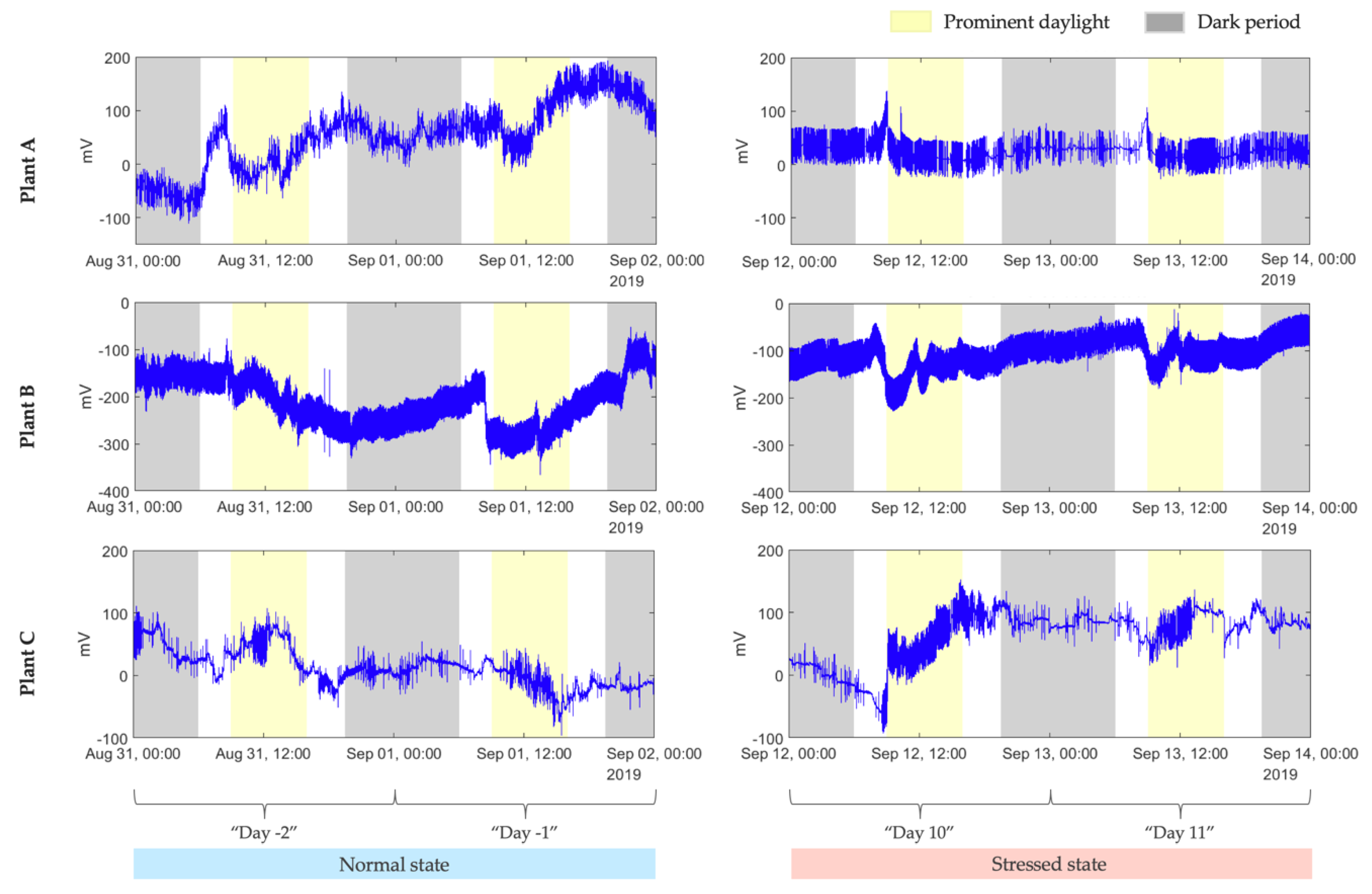
The study aims to build a model that distinguishes the normal from the stressed plant state caused by a spider mite infestation. Therefore, we chose to work with fragments of the signal of 2 days recorded before the contamination (“Day -2” and “Day -1”) and with another fragment of the same length taken before applying the phytosanitary treatment (“Day 10” and “Day 11”), from each of the 12 selected, infested plants, respectively. More precisely, the final dataset included, in total, 48 days of recordings acquired from the 12 plants, where half represented the electrophysiological signal in a normal plant state, and the other half were in a stressed state. The signals recorded from three plants that were enclosed in the taken dataset are shown in Figure 3.

2.3. Signal Preprocessing

The raw signal from the chosen dataset underwent several preprocessing steps.

Notch filtering. The signal was first filtered with band-stop filters at 50 Hz and 100 Hz, to eliminate the noise from local electrical power sources and its first harmonic, which is the only known source for eventual perturbation of the recordings. Having as aim to explore the full range of frequencies contained in the recorded signal, no other additional filtering was applied.

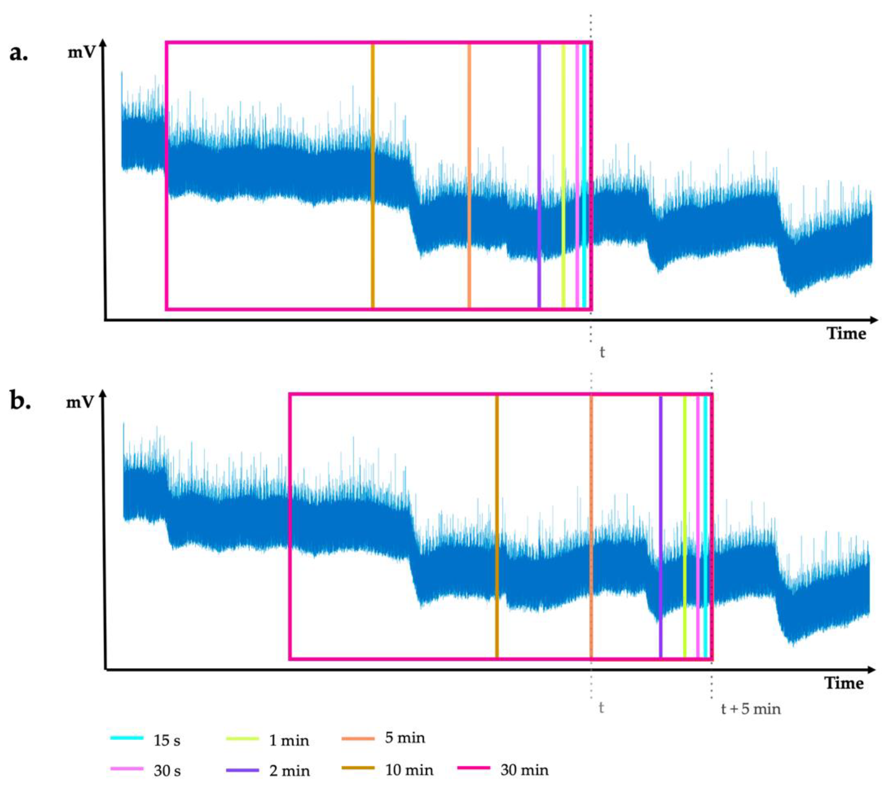
Windowing. Following normal signal processing practice, instead of exploring the entire signal waveform at once, the filtered electrical signal was initially partitioned into fragments of relatively short durations. More precisely, in a step of 5 min, seven different windows of fixed length, namely the last 15 s, 30 s, 1 min, 2 min, 5 min, 10 min and 30 min, were extracted from the signal (refer to Figure 4). As this is a relatively new domain of research, there is a lack of knowledge of the temporal extent at which the signal information characterizing the stressed plant state could be discriminated. Therefore, to explore the temporal extent in this context, rather than taking only one signal window at each sampling step, we choose to work with seven different window sizes. All of these seven windows will represent a single sample for a given plant. Hence, using this approach for the taken 96 h of recordings, we ended up with a set of 1152 samples for each plant (288 samples per single day).

Labelling. Each of the samples was labelled either as normal (‘0’) or as infested/stressed (‘1’) conforming to the meta-data information, i.e., considering the information if the sample in question was recorded before or after the contamination.

2.4. Feature Extraction

To characterize the delimited signal, for each of the chosen windows, 34 signal features were calculated using Matlab^® (version R2019b):

Time domain. Along with the main descriptive statistical features, such as mean, minimum, maximum, variance, skewness, kurtosis and interquartile range, the following other statistical features were extracted: Hjorth Mobility [22] (characterizing the mean signal slope), Hjorth Complexity [22] (signal curvature), Generalized Hurst exponent [23] (long-term memory/dependency of the signal), the logarithmic and the Shannon wavelet packet entropy, all of them previously used for the analysis of the electrical plant signals and biological signals in general [11]. To broaden the analytical tools used in plant electrophysiology, features used in other signal analysis domains were also computed. These include the root mean square of the window signal and the corresponding crest, shape, impulse and margin factor extracted as time-domain features [22,24].

Frequency domain. Aiming at identifying and characterizing the eventual spectral changes in the signal due to induced plant stress, several statistical frequency-domain features were also calculated, namely frequency center, root variance frequency (considered as the first- and second-order moment of the Fourier spectrum respectively) and the root-mean-square frequency [22].

Color Noise. As reported in recent literature [10,25,26], along with the eventual temporal dynamics, different external stimuli can change the type of color noise present in the plant electrical signal. To explore this further, we first generated the five color noises using the Matlab dsp.ColoredNoise function and calculated the corresponding fast Fourier transform (FFT). Then, we denoised the windowed signal applying the Matlab wden function (using Daubechies wavelet of order 4 and hard thresholding employing the principle of Stein’s Unbiased Risk rule and rescaled on a single estimation of noise level based on first-level coefficients). The difference between the original windowed signal and the obtained denoised signal was considered as the signal’s noise. Finally, we calculated the dot product between the normalized half-length FFT applied on the estimated noise and the normalized half-length color-noise FFT for each color noise, respectively.

Time-frequency domain. The wavelet decomposition, representing a time-frequency domain characterization of a signal, is a recommended practice for analyzing non-stationary signals enabling more accurate tracking of both changes in signal amplitude and frequency. Consequently, for each window signal, we performed wavelet decompositions of order 8 using the Matlab modwtmra function for multiresolution analysis based on maximum overlap discrete wavelet transform (output of the Matlab modwt function), which allows a higher level of information in the wavelet decomposition by avoiding the process of subsampling [27]. We selected the decomposed signal at levels 1, 4 and 8, and we calculated their respective minimum, maximum and mean values.

Table 1. Features calculated within each window for each sampling step.

Extracted Features
1. Minimum	18. Minimum of the wavelet decomposition of order 1 (WD1)
2. Maximum	19. Maximum of the WD1
3. Mean	20. Mean of the WD1
4. Variance	21. Minimum of the WD4
5. Skewness	22. Maximum of the WD4
6. Kurtosis	23. Mean of the WD4
7. Interquartile Range (IQR)	24. Minimum of the WD8
8. Hjorth Mobility	25. Maximum of the WD8
9. Hjorth Complexity	26. Mean of the WD8
10. General Hurst Exponent (GHE)	27. Frequency Center
11. Logarithmic wavelet packet entropy (Logarithmic Wentropy)	28. RMS Frequency
12. Shannon wavelet packet entropy (Shannon Wentropy)	29. Root Variance Frequency
13. Root Mean Square (RMS)	30. White Noise
14. Crest Factor	31. Pink Noise
15. Shape Factor	32. Brown Noise
16. Impulse Factor	33. Blue Noise
17. Margin Factor	34. Purple Noise

lists the 34 calculated features for each of the seven windows. In total, 238 features per sample were extracted. The concatenation of all the 238 features from the 12 plants led to a total of 13,824 samples to analyze, with exactly half labelled as “normal” and half labelled as “stressed”.

2.5. Features Subsets

The relatively high number of extracted features could potentially lead to overfitting by the model. Moreover, as for every window length, the 34 features represent the same measures calculated at a different scale, a strong correlation between them could also occur.

To further assess the impact of the feature space dimension on the classification accuracy, two feature subsets were considered in the analysis:

• The original set enclosing all the 238 features;
• The set of mutually uncorrelated features (correlation < 95%, significance level = 5%) where each one of them is correlated with the label vector (correlation > 1%). Among them, we excluded as well those which are nearly constant over time (the number of occurrences of its most frequent value is bigger than 90% of the number of samples).

Additionally, since it is a relatively new field of research, we aimed to assess the most important features for the classification.

2.6. Samples Subsets

Observation of the recordings suggested that there may be differences in the electrophysiological response during hours of daylight (photosynthesizing) and hours of darkness (respiring). To test if reactions to the infestation were different during these periods, two different sample subsets were considered: one containing only samples recorded during prominent daylight and the other one formed from samples recorded in the absence of sunlight (refer to Figure 3). The dawn and the dusk samples were not included in either of these two subsets.

The acquisitions were made in an alpine region, and the actual sunrise and sunset are impacted by geography; therefore, the dawn and the dusk last longer. We used the greenhouse’s climatic monitoring device DGT-Senmatic (Senmatic, Industrivej 8, 5471 Søndersø, Denmark) to measure the light intensity to determine the actual daylight period. At this time of the year, the daylight period is between 9 a.m. and 4 p.m., during which the sun irradiation is over 100 W/m², and night is between 7:30 p.m. and 6 a.m. (with 0 W/m²).

For all four chosen days of recordings, 336 samples were obtained from each plant during daylight, or 4032 samples in total. To avoid introducing a bias regarding the size of the two subsets, 4032 samples in total were also chosen to form the night subset. More precisely, for each plant we took 168 samples from the dark period nearest the end of the recording in normal state and the 168 samples from the dark period nearest the end of the recording in the stressed state.

Additionally, as in the case when enclosing all of the extracted 13,824 samples, both the daylight and the night subsets contained an equal number of samples from the pre-infested (normal) and the stressed state.

2.7. Features Normalization

To compensate for inter-plant variability, each feature vector was normalized using the min–max normalization method based on the recorded values of the respective plant, which brought all the feature values to the interval [0, 1].

2.8. Classification Model Development

A preliminary investigation showed that a Gradient Boosted Tree (GBT) algorithm [28], a machine learning technique that uses an ensemble of decision trees to address a regression or a classification problem, provides better classification performance than other tested algorithms such as Logistic Regression, Decision Trees, Deep Learning and Random Forest [15]. Hence, for this study, the GBT algorithm was chosen to build the classification model. For this task, we used the software platform RapidMiner Studio, version 9.6.

Throughout the modeling process, the data were first divided into subsets for training the model and for validating the model. The training subset included 75% of the total samples, whereas the remaining 25% represented the test set. The latter was used to evaluate the performance of the classifier learnt during the training phase or, more precisely, to estimate the classifier accuracy, specificity, recall and precision values.

-

Accuracy: the ratio between the number of correctly predicted samples and the total number of samples;

-

Precision: the proportion of correctly predicted samples of a chosen class among all the samples predicted as samples of that class;

-

Recall (or Sensitivity): the proportion of correctly predicted samples of a chosen class among all the samples from that class;

-

Specificity: the rate of correctly rejected samples for predicting a chosen class in binary classification.

The test set was first divided into seven randomly chosen subsets with approximately equal size, and the model was applied on each one of them. The obtained results allowed the identification and then the exclusion of the two subsets, among the seven, on which the model performed with the highest and the lowest accuracy, respectively. The final results represent the average performance of the model applied to the remaining five subsets.

Given that there could be an important correlation between samples from the same plant, to avoid bias in evaluating the model’s performance, the training set was built on samples from 9 of the 12 plants, whereas the test set was built from the remaining 3 plants. The plants in each subset were randomly chosen, but it was assured that the test set was composed of plants recorded with different acquisition devices.

During the training phase, the main GBT parameters—number of trees, maximum depth, and learning rate—were tuned within a grid search. The tested values for number of trees were [100, 200, 300], the maximal depth [4, 7, 9], and the learning rate [0.05, 0.1 and 0.3]. Hence, 27 possible combinations of these parameters’ values were evaluated.

The procedure of learning the optimal combination of parameters involved a nine-fold customized cross-validation process, nine being the number of plants whose samples were enclosed in the training set. More precisely, for a given combination of the three parameters, the original training set was subdivided into two subsets: (1) a set for learning the model containing only the samples of eight out the nine plants and (2) a test set for evaluating the learnt model enclosing the samples of the remaining ninth plant. Keeping the same parameter values, this procedure was repeated nine times in a way that the samples of each plant will represent the test set once only. At the end, the parameters’ values are chosen by the combination giving the highest classification accuracy in average for all nine folds. The presented workflow could be generalized for an n-fold cross-validation approach, where n represents the number of plants in the training set.

3. Results

Observations of the recorded signals led us to investigate whether insect activity and plant responses were the same during daylight and night time. Models for distinguishing the normal from the stressed state of the plant, all based on a GBT algorithm, showed distinctive performance for three different samples subsets: (i) all data, (ii) samples from daylight period and (iii) samples from the night time. In general, for all of the sample subsets, decreasing the number of features showed a low impact on the accuracy of the models.

3.1. Original Set of Samples

The models built from the original set enclosing all of the samples with equal distribution of the two classes, normal and stressed state, showed fair discriminative efficiency.

Original set of features. By using all of the 238 extracted features, the optimal combination of GBT parameters included 100 as the number of trees, 7 as the maximal depth and 0.05 as the learning rate. The model applied on the test data set of samples showed an accuracy of 69.8% ± 0.6%. Figure S1 in the Supplementary Material shows the obtained prediction for each sample forming the respective test set. The first five features appearing as most discriminative for the classification with the GBT algorithm were IQR calculated within a window of 2 min (relative importance weight: 19.4%), modelization of purple noise at 30 min (6.4%), GHE at 30 min (6.3%) and the Hjorth complexity at 2 (4.2%) and 10 min (3.3%). A summary of the obtained most discriminative features is given in

Table 2. List of the five most dominant features used by the built GBT-based models to identify plant status for each of the studied scenarios.

All Samples
Original Set of Features		Reduced Set of Features
Feature	Weight	Feature	Weight
IQR 2 min	19.4%	IQR 2 min	15.5%
Purple noise 30 min	6.4%	GHE 30 min	8.2%
GHE 30 min	6.3%	Purple noise 30 min	7.5%
Hjorth complexity 2 min	4.2%	Hjorth complexity 2 min	5.6%
Hjorth complexity 10 min	3.3%	Hjorth mobility 5 min	4.6%
Daylight Samples
Original Set of Features		Reduced Set of Features
Feature	Weight	Feature	Weight
Hjorth complexity 5 min	35.2%	Hjorth complexity 5 min	33.4%
GHE 30 min	8.9%	GHE 30 min	10.9%
Hjorth mobility 10 min	6.3%	Hjorth mobility 10 min	6.6%
Purple noise 30 min	5.7%	Margin factor 15 s	5.8%
Blue noise 30 min	4.1%	White noise 30 min	4.6%
Night Samples
Original Set of Features		Reduced Set of Features
Feature	Weight	Feature	Weight
Logarithmic wentropy 15 s	36.1%	Logarithmic wentropy 15 s	37.2%
Impulse factor 15 s	8.0%	Crest factor 15 s	11.0%
Mean of WD4 15 s	6.5%	Frequency center 15 s	5.2%
Frequency center 15 s	2.9%	Minimum 15 s	4.6%
Shape factor 30 min	2.7%	Hjorth complexity 30 s	4.3%

. On the other hand, the feature that contributed least was the mean of the wavelet decomposition of order 8 calculated for windows of different sizes (Table S1 in the Supplementary Material).

Reduced set of features. The set of mutually uncorrelated features that were, at the same time, correlated to the label-vector and varied over time contained 118 elements. The model for classification was built with 100 trees, maximum depth of 4 and 0.05 as the learning rate. The accuracy reached 70.8% ± 0.5% (Figure S2 in the Supplementary Material), and IQR at 2 min appeared as the most discriminative feature with a relative importance weight of 15.5%. It was followed by GHE at 30 min (8.2%), purple noise at 30 min (7.5%), Hjorth complexity at 2 min (5.6%) and Hjorth mobility at 5 min (4.6%). The smallest contribution comes from the minimum of the wavelet decomposition of order 4 at 30 s, GHE at 1 min, shape factor at 2 min, crest factor at 5 min and kurtosis at 10 min (Table S1).

3.2. Daylight Samples Subset

The GBT-based classifiers modeled on the set enclosing only the samples acquired during daylight showed increased efficiency of about 10%, for distinguishing the stressed- from the normal-state samples.

Original set of features. The model was built with 100 trees, 4 as maximal depth and 0.05 as the learning rate. The classification accuracy reached 80.0% ± 2.2%. The obtained prediction of each sample forming the corresponding test set is illustrated in Figure 5. The most dominant feature for the discrimination, with a relative importance weight of 35.2%, was Hjorth complexity calculated using 5 min windows. The importance of the following four features was considerably lower: GHE at 30 min (8.9%), Hjorth mobility at 10 min (6.3%), and purple (5.7%) and white noise (4.1%), both calculated at 30 min. The least dominant features were the mean of the wavelet decomposition of order 8 at 30 min and 10 min, the kurtosis at 30 min, the brown noise at 10 min and the maximum of the wavelet decomposition of order 8 at 10 min (Table S1).

Reduced set of features. The reduced set included 122 features in total. Moreover, the optimal GBT parameters remained unchanged from those obtained with the original set of features. The model showed an accuracy of 79.9% ± 1.3% (Figure S3) and relied again principally on the Hjorth complexity at 5 min for the discrimination (relative weight of importance: 33.4%). GHE calculated for windows of 30 min remained the second important feature with approximately three times smaller weight of importance (10.9%). It was followed by the Hjorth mobility at 10 min (6.6%), margin factor at 15 s (5.8%) and the white noise at 30 min (4.6%). On the opposite side the kurtosis at 30 min, the brown noise at 2 and 5 min, the RMS frequency at 5 min and the shape factor at 5 min were the features with the smallest contribution for the discrimination (Table S1).

3.3. Night Samples Subset

The models built on a set of samples recorded only during the night showed inferior results compared to the previous two scenarios.

Original set of features. The GBT model was built with 200 trees of maximum depth of 4 and 0.05 as learning rate. It classified the samples with an accuracy of 65.8% ± 0.6% (Figure S4) relying mainly on features calculated within windows of 15 s. The most discriminative appeared to be logarithmic wentropy at 15 s (36.1%), followed by impulse factor (8.0%), mean of the wavelet decomposition of order 4 (6.5%) and the frequency center (2.9%). The fifth in order was the shape factor (2.7%) calculated at 30 min. The mean of the wavelet decomposition of order 8 at 5, 10 and 30 min, together with the blue noise at 10 min and the brown noise at 5 min, were last in the order of contribution (Table S1).

Reduced set of features. Regarding this sample subset, 111 features in total formed the reduced subset of features. The GBT model built employing these features used 100 numbers of trees with a maximum depth of 4 and 0.1 as learning rate and performed with an accuracy of 65.4% ± 1.3% (Figure S5). The logarithmic wentropy calculated at 15 s appeared again as the most discriminative feature with relative importance weight of 37.2%. The following four were also from small window sizes: crest factor at 15 s (11.0%), frequency center at 15 s (5.2%), minimum at 15 s (4.6%) and the Hjorth complexity at 30 s (4.3%). The brown noise at 10 min, together with the white noise at 30 s and 1 min, the kurtosis at 1 min and the minimum of the wavelet decomposition of order 1 at 1 min, were the features with the smallest contribution (Table S1).

The results describing the performance of each classifier are summarized in

Table 3. Summary of the performance of each classification model.

Sample Set	Feature Set	Accuracy (%)	Precision * (%)	Recall * (%)	Specificity * (%)
All	Original	69.8 ± 0.6	68.4 ± 0.8	73.8 ± 1.6	65.9 ± 1.7
	Reduced	70.8 ± 0.8	71.8 ± 0.9	68.5 ± 1.5	73.0 ± 1.5
Day samples	Original	80.0 ± 2.2	80.8 ± 3.6	78.9 ± 3.0	81.1 ± 4.5
	Reduced	79.9 ± 1.3	83.8 ± 2.2	74.2 ± 2.5	85.6 ± 2.5
Night samples	Original	65.8 ± 0.9	89.9 ± 3.7	35.8 ± 3.6	95.8 ± 2.0
	Reduced	65.4 ± 1.3	84.8 ± 4.7	37.8 ± 2.7	93.1 ± 2.8

* positive class: stressed.

. The models based on signals acquired during daylight presented the highest accuracy as well as high values for the remaining performance measures regarding the prediction of the stressed states: precision, recall and specificity. On the other hand, even though the night samples models performed with high precision and specificity, its recall value, representing the sensitivity of the model, was about 36–38%; therefore, these models were very limited in predicting the stressed state (refer to Figures S4 and S5 in the Supplementary Material).

Overall, from the summary given in Table 2, one could observe that the Hjorth complexity at 5 min, IQR at 2 min and GHE at 30 min appeared as the most discriminative features. The logarithmic wentropy at 15 s appeared as an important feature for the discrimination of the plant status only when the night samples were used. Figure 6 shows the distributions without outliers of these four features for each sample subset and each window length. Hjorth complexity presented differences in distribution between the normal and the stressed state for all three sample sets and all window lengths. However, the distinction between these distributions was most notable for daylight samples, mainly for window lengths between 1 and 30 min. In the case of night samples, the Hjorth complexity distributions were notably closer. Similar findings as the Hjorth complexity feature could also be observed from the distributions of IQR. Considering GHE, distribution dissimilarities were mainly observed for the samples acquired during daylight, with most notable distinction for windows of 30 min. In line with the obtained modeling results, the logarithmic wentropy portrayed notable differences in distribution mainly for the set of night samples. For the daylight samples, these differences were very small.

Table S2 in the Supplementary Material provides a detailed list of all the features forming the reduced subsets used in these analyses. The Hjorth complexity, GHE and IQR appeared as uncorrelated features for all window lengths and all sample sets. Differently from that, the logarithmic wentropy appeared as an uncorrelated feature at 15 s and 30 min only.

4. Discussion

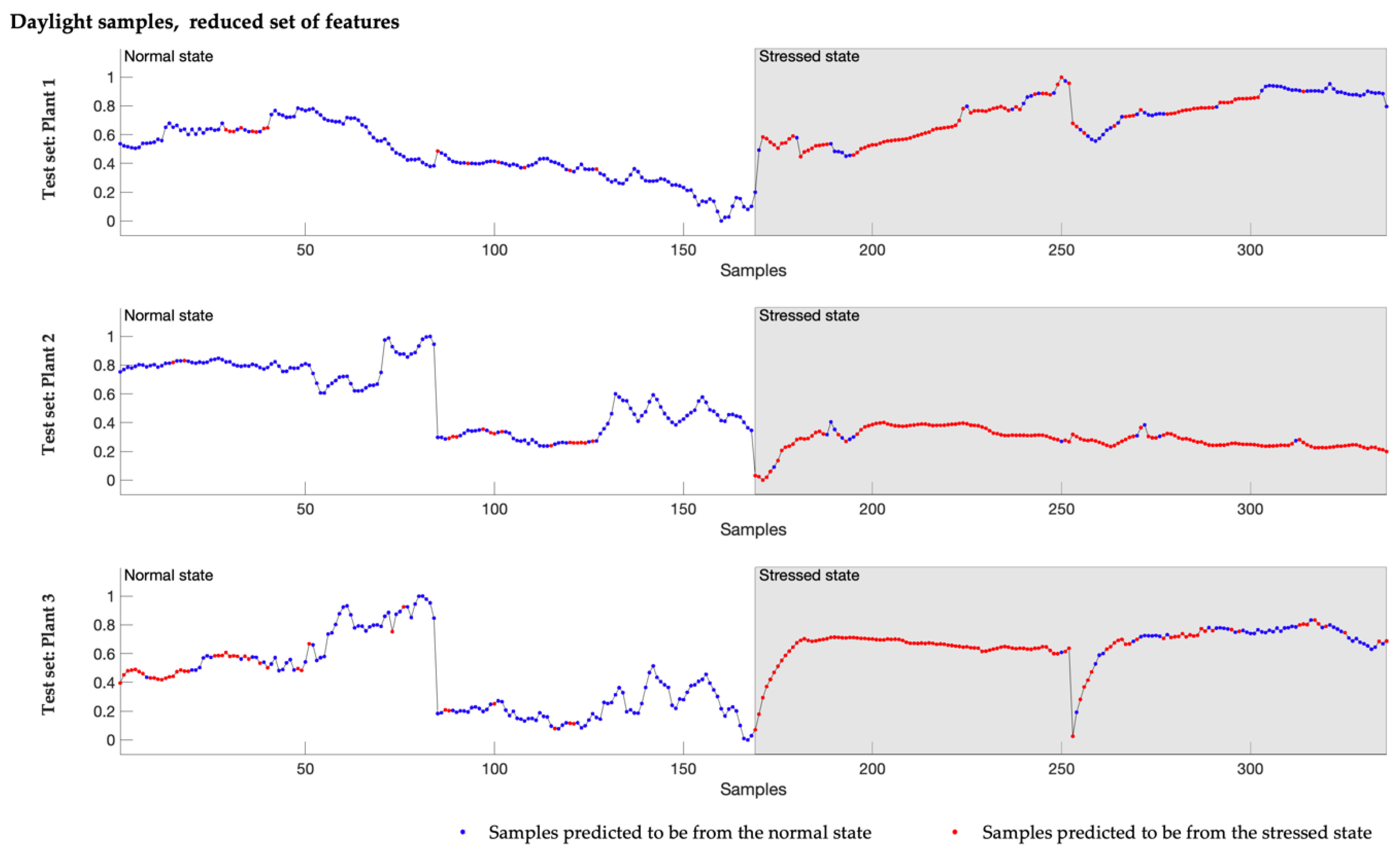
By employing machine learning techniques for data analysis, the presented exploratory study demonstrates the presence of changes in the electrophysiology signal acquired from commercial tomato plants growing in a typical production environment, caused by infestation with spider mites. It presents a methodology based on local signal features and a GBT algorithm, for modeling a classifier that is able to distinguish, with an accuracy of around 80%, the normal from the stressed plant state where the stress is induced by the infestation.

Furthermore, the study shows that models built on samples recorded during the day outperform the classifiers developed using samples, including whole 24 h cycles and, even more significantly, those based only on dark period recordings. The simultaneous high recall, precision and specificity values demonstrate the high potential of the daylight-based classifiers to distinguish between the normal and the stressed state of an infested tomato plant. In contrast, models built on the night sample sets show high precision and specificity but, at the same time, low sensitivity and therefore are more prone to predict only the normal state correctly.

It is insightful that signals collected during daylight provided a more accurate classification of plant states than either combined or nighttime-only samples. Such findings are potentially related to plant metabolism being higher during the day with water/nutrient sorption, enhanced sap flow and photosynthesis, and in consequence that plant reactions to the infestation are more pronounced during the day. Consistent with this finding, lower model performance based on samples acquired during the dark period suggests that during the night, the plant’s behavior when infested with spider mites is more similar to normal or uninfested behavior. Additionally, the improved model performance using daylight samples could also be related to increased activity of the insects during the day. Further investigation is needed to understand these differences better.

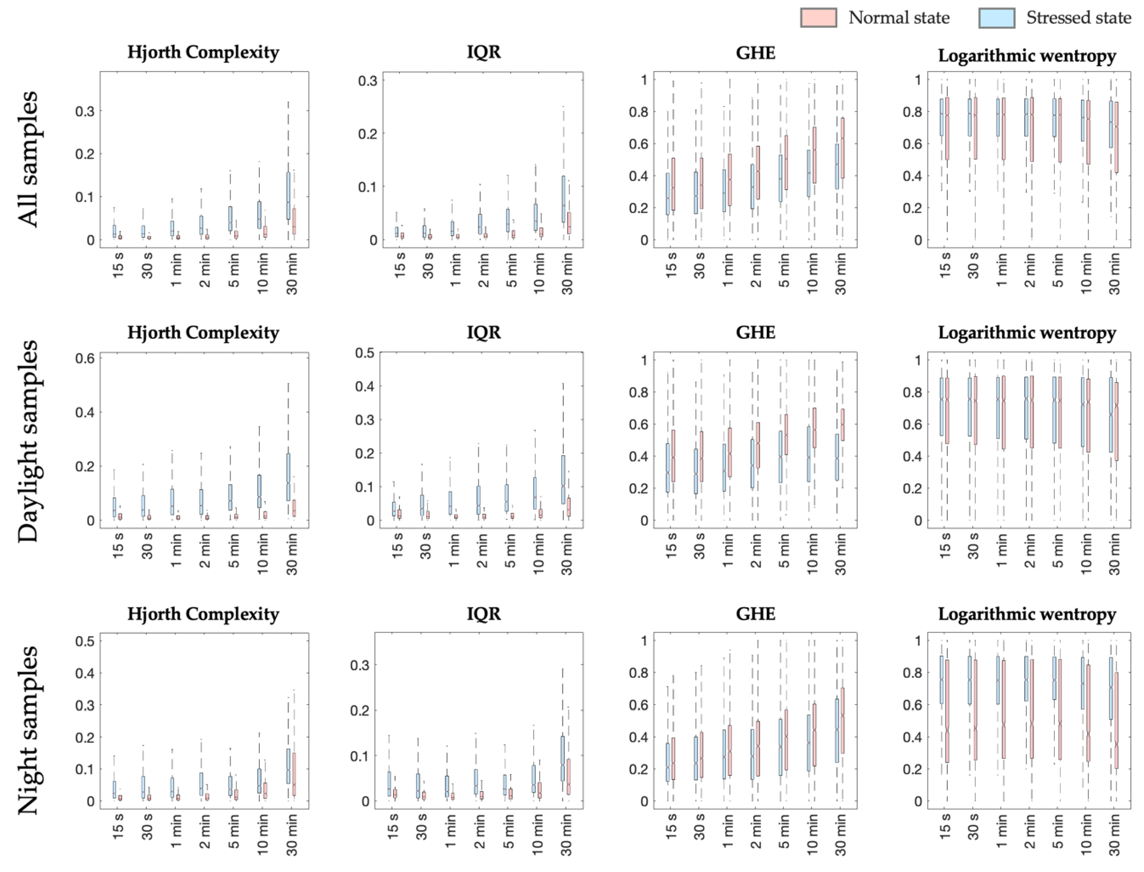
To address the lack of a priori knowledge in the domain, a relatively big specter of different signal features extracted locally was initially considered at several window lengths. With the assessment of their mutual dependency as well as their impact in the classification process, the most relevant features for the stressed state discrimination were revealed. The overall results showed that the Hjorth complexity, characterizing the considered signal’s curvature, contributes the most for the identification of the plant state within a frame of spider mites infestation.

Aside from the Hjorth complexity, the interquartile range and the General Hurst Exponent also appear as valuable features for the plant state’s discrimination. Each of these three features provides particular independent information at all the seven studied signal window lengths for the three sets of samples. Additionally, they are all portraying a temporal characterization of the signal. Hjorth complexity and IQR have previously been reported as a dominant feature for environmental stimuli discrimination when using the electrical plant response [11].

Frequency-related features, such as the color noises, also contribute to the classification of the plant state. Even though their impact is less dominant, the discriminative information they present could, however, be related to the expectations that an external stimulus is triggering a different color noise in the plant electrical response [10,25,26].

Different window lengths could also affect the discrimination power of a feature in a non-uniform manner. Additionally, the features found as the most important for the classification represent different window extents. Nevertheless, these findings suggest that to predict the plant state correctly when attacked by spider mites, signal samples of several minutes up to half an hour are most effective. The spider mites have needle-shaped mouthparts that allow them to feed by penetrating the plant tissue, which causes plant damage that is perceived locally. However, depending on the severity of the damage, the presence of spider mites induce long-distance electrical signaling through the entire plant [29,30,31].

The reduction in the features space only slightly affected the classification performance. However, with the decrease in the number of features, both the model’s complexity and its tendency to overfit also decreased. Another advantage of using fewer features is the reduction in the computational time required to build the model and to apply it on newly acquired data from other plants, conforming with the needs of the crop producers.

The isolation between the plants used for the training from those used in the testing increases the objectivity of the performance assessment and strengthens the evaluation of each model. Therefore, the built classifiers are expected to perform similarly for new recordings coming from other tomato plants.

Further studies should include an extended cohort of tomato plants to confirm the presented findings, and their reproducibility should be investigated for other growth seasons and other crops as well. Another improvement would include modeling of several stages of stress, for example, initial, middle and strong stress, which would allow greater precision in detecting plant status and, potentially, a detection of a spider mite infestation before the appearance of visual symptoms.

Another valuable contribution would be to understand more profoundly the changes in the plant occurring at cellular level. Among early signaling events that occur in response to biotic stress, electrical variations can be highlighted; it is crucial for induction of appropriate physiological modifications such as genetic regulation, metabolism adaptation, hormone synthesis or defense mechanisms [31,32]. Moreover, ion fluxes, apoplastic pH modification, ROS generation and calcium variations are responsible for electrical signaling [33,34]. Hence, investigations on how transporters contribute to slow and long-term bioelectrical potential variations would help in modeling. For instance, as in the studies of the current literature based on ancestral alga Chara demonstrating the presence of a characteristic red noise triggered by a salinity stress and mediated through H⁺/OH⁻ channels [26,35,36], such investigation would allow to discern the transporters causing alterations in the tomato electrophysiological signal in the presence of spider mites. By expending the knowledge of plant electrical responses in that context, the choice of signal features to use for an automated detection of changes in plant state could be further refined, which would also potentially lead to an accurate classification even for an early stage of infestation.

Overall, the presented findings in this study represent a starting point of building new possibilities for more optimal preventive and curative crop protection practices.

5. Patents

Patent application with reference UK1903652.4 and entitled “Electrophysiological assessment of plant status using supervised machine learning” is under review. Filed in 2019.

References

1. Culliney, T. Crop Losses to Arthropods. In Integrated Pest Management; Springer: Dordrecht, The Netherlands, 2014; Volume 3, pp. 201–225. [Google Scholar]
2. Savary, S.; Willocquet, L.; Pethybridge, S.J.; Esker, P.; McRoberts, N.; Nelson, A. The global burden of pathogens and pests on major food crops. Nat. Ecol. Evol. 2019, 3, 430–439. [Google Scholar] [CrossRef]
3. Santamaria, M.E.; Arnaiz, A.; Rosa-Diaz, I.; González-Melendi, P.; Romero-Hernandez, G.; Ojeda-Martinez, D.A.; Garcia, A.; Contreras, E.; Martinez, M.; Diaz, I. Plant Defenses Against Tetranychus urticae: Mind the Gaps. Plants 2020, 9, 464. [Google Scholar] [CrossRef] [Green Version]
4. Agut, B.; Pastor, V.; Jaques, J.A.; Flors, V. Can Plant Defence Mechanisms Provide New Approaches for the Sustainable Control of the Two-Spotted Spider Mite Tetranychus urticae? Int. J. Mol. Sci. 2018, 19, 614. [Google Scholar] [CrossRef] [PubMed] [Green Version]
5. Gutierrez, A.; Ansuategi, A.; Susperregi, L.; Tubío, C.; Rankić, I.; Lenža, L. A Benchmarking of Learning Strategies for Pest Detection and Identification on Tomato Plants for Autonomous Scouting Robots Using Internal Databases. J. Sens. 2019, 2019, 5219471. [Google Scholar] [CrossRef]
6. Bolton, M.D. Primary metabolism and plant defense—Fuel for the fire. Mol. Plant-Microbe Interact. MPMI 2009, 22, 487–497. [Google Scholar] [CrossRef] [Green Version]
7. Dangl, J.L.; Jones, J.D.G. Plant pathogens and integrated defence responses to infection. Nature 2001, 411, 826–833. [Google Scholar] [CrossRef]
8. Ramirez-Prado, J.S.; Abulfaraj, A.A.; Rayapuram, N.; Benhamed, M.; Hirt, H. Plant Immunity: From Signaling to Epigenetic Control of Defense. Trends Plant Sci. 2018, 23, 833–844. [Google Scholar] [CrossRef] [PubMed]
9. Volkov, A.G.; Ranatunga, D.R.A. Plants as Environmental Biosensors. Plant Signal. Behav. 2006, 1, 105–115. [Google Scholar] [CrossRef] [PubMed] [Green Version]
10. Pereira, D.R.; Papa, J.P.; Saraiva, G.F.R.; Souza, G.M. Automatic classification of plant electrophysiological responses to environmental stimuli using machine learning and interval arithmetic. Comput. Electron. Agric. 2018, 145, 35–42. [Google Scholar] [CrossRef] [Green Version]
11. Chatterjee, S.K.; Das, S.; Maharatna, K.; Masi, E.; Santopolo, L.; Mancuso, S.; Vitaletti, A. Exploring strategies for classification of external stimuli using statistical features of the plant electrical response. J. R. Soc. Interface 2015. [Google Scholar] [CrossRef]
12. Chatterjee, S.K.; Malik, O.; Gupta, S. Chemical Sensing Employing Plant Electrical Signal Response-Classification of Stimuli Using Curve Fitting Coefficients as Features. Biosensors 2018, 8, 83. [Google Scholar] [CrossRef] [Green Version]
13. Qin, X.-H.; Wang, Z.-Y.; Yao, J.-P.; Zhou, Q.; Zhao, P.-F.; Wang, Z.-Y.; Huang, L. Using a one-dimensional convolutional neural network with a conditional generative adversarial network to classify plant electrical signals. Comput. Electron. Agric. 2020, 174, 105464. [Google Scholar] [CrossRef]
14. Simmi, F.Z.; Dallagnol, L.J.; Ferreira, A.S.; Pereira, D.R.; Souza, G.M. Electrome alterations in a plant-pathogen system: Toward early diagnosis. Bioelectrochemistry 2020, 133, 107493. [Google Scholar] [CrossRef]
15. Tran, D.; Dutoit, F.; Najdenovska, E.; Wallbridge, N.; Plummer, C.; Mazza, M.; Raileanu, L.E.; Camps, C. Electrophysiological assessment of plant status outside a Faraday cage using supervised machine learning. Sci. Rep. 2019, 9, 17073. [Google Scholar] [CrossRef]
16. Zimmermann, M.R.; Maischak, H.; Mithöfer, A.; Boland, W.; Felle, H.H. System Potentials, a Novel Electrical Long-Distance Apoplastic Signal in Plants, Induced by Wounding. Plant Physiol. 2009, 149, 1593. [Google Scholar] [CrossRef] [PubMed] [Green Version]
17. Choi, W.-G.; Hilleary, R.; Swanson, S.J.; Kim, S.-H.; Gilroy, S. Rapid, Long-Distance Electrical and Calcium Signaling in Plants. Annu. Rev. Plant Biol. 2016, 67, 287–307. [Google Scholar] [CrossRef] [PubMed]
18. Farmer, E.E.; Gao, Y.-Q.; Lenzoni, G.; Wolfender, J.-L.; Wu, Q. Wound- and mechanostimulated electrical signals control hormone responses. New Phytol. 2020, 227, 1037–1050. [Google Scholar] [CrossRef] [PubMed]
19. Gigon, V.; Camps, C.; Le Corff, J. Biological control of Tetranychus urticae by Phytoseiulus macropilis and Macrolophus pygmaeus in tomato greenhouses. Exp. Appl. Acarol. 2016, 68, 55–70. [Google Scholar] [CrossRef]
20. Jovanov, E.; Volkov, A.G. Plant Electrostimulation and Data Acquisition. In Plant Electrophysiology; Springer: Berlin/Heidelberg, Germany, 2012. [Google Scholar]
21. Kurenda, A.; Stolarz, M.; Zdunek, A. Electrical potential oscillations—Movement relations in circumnutating sunflower stem and effect of ion channel and proton pump inhibitors on circumnutation. Physiol. Plant. 2015, 153, 307–317. [Google Scholar] [CrossRef]
22. Caesarendra, W.; Tjahjowidodo, T. A Review of Feature Extraction Methods in Vibration-Based Condition Monitoring and Its Application for Degradation Trend Estimation of Low-Speed Slew Bearing. Machines 2017, 5, 21. [Google Scholar] [CrossRef]
23. Aste, T. Generalized Hurst Exponent. MATLAB Central File Exchange. 2013. Available online: https://www.mathworks.com/matlabcentral/fileexchange/30076-generalized-hurst-exponent (accessed on 23 January 2019).
24. Ben Ali, J.; Saidi, L.; Harrath, S.; Bechhoefer, E.; Benbouzid, M. Online automatic diagnosis of wind turbine bearings progressive degradations under real experimental conditions based on unsupervised machine learning. Appl. Acoust. 2018, 132, 167–181. [Google Scholar] [CrossRef]
25. Souza, G.M.; Ferreira, A.S.; Saraiva, G.F.R.; Toledo, G.R.A. Plant “electrome” can be pushed toward a self-organized critical state by external cues: Evidences from a study with soybean seedlings subject to different environmental conditions. Plant Signal. Behav. 2017, 12, e1290040. [Google Scholar] [CrossRef] [Green Version]
26. Al Khazaaly, S.; Alan Walker, N.; Beilby, M.J.; Shepherd, V.A. Membrane potential fluctuations in Chara australis: A characteristic signature of high external sodium. Eur. Biophys. J. 2009, 39, 167–174. [Google Scholar] [CrossRef]
27. Ghaemi, A.; Rezaie-Balf, M.; Adamowski, J.; Kisi, O.; Quilty, J. On the applicability of maximum overlap discrete wavelet transform integrated with MARS and M5 model tree for monthly pan evaporation prediction. Agric. For. Meteorol. 2019, 278, 107647. [Google Scholar] [CrossRef]
28. Chen, T.; Guestrin, C. XGBoost: A Scalable Tree Boosting System. In Proceedings of the 22nd ACM SIGKDD International Conference on Knowledge Discovery and Data Mining—KDD ’16, San Francisco, CA, USA, 13–17 August 2016. [Google Scholar]
29. Toyota, M.; Spencer, D.; Sawai-Toyota, S.; Jiaqi, W.; Zhang, T.; Koo, A.J.; Howe, G.A.; Gilroy, S. Glutamate triggers long-distance, calcium-based plant defense signaling. Science 2018, 361, 1112. [Google Scholar] [CrossRef] [PubMed]
30. Muday, G.K.; Brown-Harding, H. Nervous system-like signaling in plant defense. Science 2018, 361, 1068. [Google Scholar] [CrossRef] [PubMed]
31. Mousavi, S.A.R.; Chauvin, A.; Pascaud, F.; Kellenberger, S.; Farmer, E.E. GLUTAMATE RECEPTOR-LIKE genes mediate leaf-to-leaf wound signalling. Nature 2013, 500, 422–426. [Google Scholar] [CrossRef] [Green Version]
32. Wendehenne, D.; Lamotte, O.; Frachisse, J.-M.; Barbier-Brygoo, H.; Pugin, A. Nitrate Efflux Is an Essential Component of the Cryptogein Signaling Pathway Leading to Defense Responses and Hypersensitive Cell Death in Tobacco. Plant Cell 2002, 14, 1937. [Google Scholar] [CrossRef] [PubMed] [Green Version]
33. Tran, D.; Dauphin, A.; Meimoun, P.; Kadono, T.; Nguyen, H.T.H.; Arbelet-Bonnin, D.; Zhao, T.; Errakhi, R.; Lehner, A.; Kawano, T.; et al. Methanol induces cytosolic calcium variations, membrane depolarization and ethylene production in arabidopsis and tobacco. Ann. Bot. 2018, 122, 849–860. [Google Scholar] [CrossRef]
34. Haapalainen, M.; Dauphin, A.; Li, C.-M.; Bailly, G.; Tran, D.; Briand, J.; Bouteau, F.; Taira, S. HrpZ harpins from different Pseudomonas syringae pathovars differ in molecular interactions and in induction of anion channel responses in Arabidopsis thaliana suspension cells. Plant Physiol. Biochem. 2012, 51, 168–174. [Google Scholar] [CrossRef] [PubMed]
35. Al Khazaaly, S.; Beilby, M.J. Zinc ions block H+/OH- channels in Chara australis. Plant Cell Environ. 2012, 35, 1380–1392. [Google Scholar] [CrossRef] [PubMed]
36. Absolonova, M.; Beilby, M.J.; Sommer, A.; Hoepflinger, M.C.; Foissner, I. Surface pH changes suggest a role for H+/OH channels in salinity response of Chara australis. Protoplasma 2018, 255, 851–862. [Google Scholar] [CrossRef] [PubMed] [Green Version]
Figure 1. Plant infestation with spider mites. Panel (a) illustrates the process of infestation where each plant was inoculated with 30 mobile stage of spider mites put on a cotton pad that was attached on the leaves. Panels (b,c) show the appearance of infested tomato leaves when the plants presented strong stress related to the infestation.
Applsci 11 01414 g001
Figure 2. Acquisition of the plant electrophysiology signal. The left panel shows a schematic representation of the setup used for measuring the electrical potential from each plant, whereas the right panel gives a closer look at the used recording device and the electrodes inserted on the plant.
Applsci 11 01414 g002
Figure 3. Recorded signal from three plants included in the analyzed dataset (after a band-filtering at 50 Hz and 100 Hz). “Day -2” and “Day -1” represent the two days before the contamination of the plants, whereas “Day 10” and “Day 11” are the tenth and eleventh days after the contamination. The light yellow indicates the periods of the day where there was prominent daylight, whereas the grey indicates the dark periods.
Applsci 11 01414 g003
Figure 4. Schematic representation of the windowing procedure. At time point t (panel (a)) seven intervals of different lengths are taken from the signal, namely the last 15 s, 30 s, 1 min, 2 min, 5 min, 10 min and 30 min. Once the features are calculated for all of these seven windows, we move forward in a step of 5 min (panel (b)), where we take seven new intervals of the recorded signal with the same lengths as in the previous step. This procedure is repeated to cover the entire duration of the signal recording.
Applsci 11 01414 g004
Figure 5. Predicted class of each sample forming the test set used to evaluate the model obtained when analyzing the daylight samples subset with the reduced set of features. The color of the samples indicates the class that has been attributed to them by the classification model—blue represents the normal, whereas red is the stressed state. For each plant, the plotted samples overlay the normalized feature mean value of the signal calculated for a window of 5 min.
Applsci 11 01414 g005
Figure 6. Distribution of the four features observed as the most discriminative for the GBT classification. Each of them is represented without outliers for all the three explored sets of samples and all window lengths.
Applsci 11 01414 g006