Structural Health Monitoring of 2D Plane Structures

Abstract

This paper presents the application of the observability technique for the structural system identification of 2D models. Unlike previous applications of this method, unknown variables appear both in the numerator and the denominator of the stiffness matrix system, making the problem non-linear and impossible to solve. To fill this gap, new changes in variables are proposed to linearize the system of equations. In addition, to illustrate the application of the proposed procedure into the observability method, a detailed mathematical analysis is presented. Finally, to validate the applicability of the method, the mechanical properties of a state-of-the-art plate are numerically determined.

1. Introduction

In recent years, the maintenance, health monitoring, and identification of structural systems are becoming more frequent all around the world [1,2]. A methodology to identify the mechanical properties of existing structures according to in situ measurements is defined as structural system identification [3] and is a necessary part of any Structural Health Monitoring system. In the maintenance and rehabilitation process of the structures, in addition to the in situ measurements and visual inspections, precise damage detection might be performed using numerical and analytical analysis [4,5]. Examples of non-model-based damage identification approaches can be found in [6,7].

Many structural system identification methods have been proposed for estimating the mechanical parameters of structures modelled with 1D elements, such as steel and concrete buildings as well as cable-stayed bridges, trusses, and frames [8,9,10]. However, despite the intricate nature of 2D structural models such as tunnels, dams, and culverts, few investigations have been conducted on the structural system identification of these structures [11,12,13,14,15]. For instance, geotechnical engineers who tried to estimate the behavior of buried structures encountered insufficient sets of input data [16,17]. In the case of segmental underground structures, both the constraining effect of the soil and the existence of the segment joints will generate problems for acquiring dynamic characteristics [18,19,20]. Khamsei et al. presented a new intelligent inverse analysis technique combining fuzzy systems, an imperialistic competitive algorithm, and numerical analysis for the back analysis of the Karaj Subway in Iran [21]. Dehghan et al. determined the geotechnical parameters using inverse analysis based on convergence data [22]. They also proved that their proposed method would be a more economical and time-saving technique in comparison to a design based on soil mechanic tests carried out by consultant engineers.

Structural system identification methods can be categorized as parametric and non-parametric [23,24,25]. With the quick increase in computer technology, jutting numerical software, and well-known packages such as MatLab or Mathematica, the popularity of non-parametric methods has increased. These methods define the transfer functions of a system, which implies that the input–output relation is characterized by a set of equations that may not have any explicit physical meaning. Vardakos et al. estimated the potential use of the differential evolution genetic algorithm in the back analysis of a tunnel response to obtain improved estimates of the model parameters by matching the model prediction with the monitored response [25].

Xiang et al. proposed two algorithms by means of automatically generating optimal measurements [26]. They proved the validity of their methods with academic examples. They used their proposed method for the Munich subway tunnel project. Santos et al. presented a procedure to carry out back analysis of the tunnel excavation problem in an automatic manner [27]. They verified their measurements with ones obtained from a finite element analysis. However, in parametric methods all the parameters have physical meaning in the equations and may be used as a method to identify the parameters of the structures. Lozano-Galant et al. proposed a parametric method to uniquely identify the mechanical properties of structures as well as the flexural and axial stiffness (EA, EI) [28]. This technique is called the observability method (OM) and is enforceable for the structural system identification of 1D elements (Bernoulli and Timoshenko beam elements) but not for finite element models with 2D elements.

OM stands as one of the unique structural system identification parametric approaches presented in the literature for the static [29,30,31,32,33,34,35,36] and dynamic analysis of the stiffness matrix method [37]. The advantages of using this deterministic and physics-based approach are: 1—the mathematical foundation of the technique is simple and comprehensible; 2—OM defines whether all the variables or a subset of them are observable or not; 3—OM permits engineers to acquire unique solutions of a structural system in a reasonable time; 4—OM allows the identification of the mechanical parameters of the structure even if the involved parameters are not linearly related; 5—if there is not a unique solution for a specific part of a system, with a quick evaluation of the system relations are obtained that allow the user to specify which measurements must be obtained to have more or complete observability [38].

OM was applied satisfactorily to solve engineering structural problems. For instance, Lozano-Galant et al. facilitated the application of OM for the identification of the parameters of complex concrete and steel bridges by proposing a graphical method for the selection of measurement sets, which is called observability trees [34]. The use of observability trees proved that, in the analyzed system, the probability of selecting the appropriate measurement set with a minimum number of measurements at random was practically negligible. In addition, Castillo et al. utilized OM to assist in decision-making and risk management processes during the maintenance and service life of structures [30].

Although it has applicability to many structures, OM has never been applied to models made out of 2D elements. Along with the undertaken studies and the proposed existing gaps, for the first time we propose a new system of equation for the application of OM to the inverse analysis of 2D models. This application is not as straightforward as it might look. The 1D OM unknowns (Young’s modulus E, area A, Inertia I, and flexural or axial stiffnesses) are located only in the numerator of the stiffness matrix [28]. However, for the implementation of 2D models an obstacle arises, as the Poisson ratio appears in the both the numerator and the denominator of the elements of the stiffness matrix. This location of unknowns creates a nonlinear system of equations that prevents defining the unknowns through traditional OM. The location of the unknowns creates a non-linear system of equations that prevents the identification of the mechanical properties of the 2D element structures with the traditional OM. To solve this problem, this paper proposes a new methodology to enable the application of the OM to 2D model structures. The main contribution of this work refers to the use of changes in variables to linearize non-linear systems of equations. To illustrate the introduction of this change of variable into the observability method, a detailed mathematical analysis is presented. Finally, to validate the applicability of the method, the mechanical properties of a state-of-the-art plate are numerically determined. It is important to highlight that the proposed mathematical methodology is characterized by its generality, as it can be used for other systems of equations, including unknown variables in both the numerator and the denominator. With the proposed methodology, scholars can derive the mechanical parameters of crucial structures, such as tunnels, gravity dams, retaining walls, buttress dams, culverts, and underground pipelines.

This paper is organized as follows. In Section 2, the observability technique is elucidated and we demonstrate how it could be exerted to the stiffness matrix method of 2D elements. In Section 3, an example of a state-of-the-art technique is analyzed to show the applicability of OM to 2D element structures. Moreover, a statistical analysis of the required number of measurements for reaching different levels of observability is shown in this section. Finally, the conclusions of the article are presented in Section 4.

2. Structural System Identification of Structures with 2D Elements by Observability Techniques

In this section, the application of the observability method (OM) to the inverse analysis of structures modeled by 2D elements is firstly described. Then, the proposed algorithm to implement the application of the OM to 2D element structures is presented. Finally, the differences in the system of equations of structures with 1D and 2D elements are reviewed.

2.1. Inverse Analysis of the Stiffness Matrix Method

According to the Finite Element Method ([39]), the stiffness matrix of 2D element structures [K] can be obtained from the strain-displacement matrix [B] and elastic matrix [D], as presented in Equation (1):

$$\left[\mathrm{K}\right]={{\displaystyle \mathrm{\int }}}_{\mathrm{V}}{\left[\mathrm{B}\right]}^{\mathrm{T}}\left[\mathrm{D}\right]\left[\mathrm{B}\right] \mathrm{dV}.$$

(1)

In the stiffness matrix method, matrix [K] is used to relate the equilibrium equations in terms of the nodal displacements, as presented in Equation (2).

$${\left[\mathrm{K}\right]}^{\left(2{\mathrm{N}}_{\mathrm{N}}\times 2{\mathrm{N}}_{\mathrm{N}}\right)}·{\left\{\mathsf{\delta }\right\}}^{\left(2{\mathrm{N}}_{\mathrm{N}}\times 1\right)}={\left\{\mathrm{f}\right\}}^{\left(2{\mathrm{N}}_{\mathrm{N}}\times 1\right)},$$

(2)

where, [K] depends on the following characteristics: thickness (h), Young’s modulus ($\mathrm{E}$), and Poisson ratio ($\vartheta$). $\left\{\mathsf{\delta }\right\}$ is the vector of displacements, which includes the vertical (${\mathrm{v}}_{\mathrm{i}}$) and horizontal (${\mathrm{u}}_{\mathrm{i}}$) deflections at each node i, and $\left\{\mathrm{f}\right\}$ is the force vector that contains the vertical (${\mathrm{V}}_{\mathrm{i}}$) and horizontal (${\mathrm{H}}_{\mathrm{i}}$) applied forces at each node i. Finally, ${\mathrm{N}}_{\mathrm{N}}$ refers to the number of nodes in the finite element equation. For the case of tunnel, dam, and culvert analysis, the plane strain assumption is traditionally considered and the thickness is assumed as one.

In the traditional application of the stiffness matrix method, the parameters in [K] are known and the nodal displacements can be directly obtained from Equation (2). Then, the internal forces in the elements as well as the reactions at the boundary conditions can be obtained from these displacements. This methodology is traditionally used by computer software to simulate the structural responses. A detailed explanation of the application of this approach can be found in [38].

The stiffness matrix method can be also used to identify unknown mechanical properties of the structural elements (e.g., ${\mathrm{h}}_{\mathrm{j}}$, ${\vartheta }_{\mathrm{j}}$, ${\mathrm{E}}_{\mathrm{j}}$) from the structural response measured on site (inverse approach). In this approach, some terms in the stiffness matrix are assumed as unknown together with the reactions at the boundary conditions and the unmeasured deflections on site. In this inverse approach, non-linear products of unknown variables appear. To identify these non-linear products of unknown in 1D element structures, the OM was proposed in the literature. This method requires the rearrangement of the system of equations of the stiffness matrix method to join all the unknown variables together. To do so, the system in Equation (2) can be reordered as follows [28]:

$${\left[\mathrm{K}\right]}^{*}·{\left\{\mathsf{\delta }\right\}}^{*}=\left\{\mathrm{f}\right\},$$

(3)

where, the products of variables are located in the modified vector of displacements {δ*} and the modified stiffness matrix [K]* is a matrix of coefficients with different dimensions than the initial stiffness matrix [K]. Once the boundary conditions and the applied forces at the nodes during the nondestructive test are introduced, it can be assumed that a subset of deflections δ₁* of {δ*} and a subset of forces in nodes f₁ of {f} are known and the remaining subset δ₀* of {δ*} and f₀ of {f} are unknown. By the static condensation procedure, the system in (3) can be partitioned as follows [28]:

$${\left[K\right]}^{*}·\left\{{\mathsf{\delta }}^{*}\right\}=\left[\begin{array}{cc}{\mathrm{K}}_{00}^{*}& {\mathrm{K}}_{01}^{*}\\ {\mathrm{K}}_{10}^{*}& {\mathrm{K}}_{11}^{*}\end{array}\right]·\left\{\begin{array}{c}{\mathsf{\delta }}_0^{*}\\ {\mathsf{\delta }}_1^{*}\end{array}\right\}=\left\{\begin{array}{c}{\mathrm{f}}_0\\ {\mathrm{f}}_1\end{array}\right\}=\left\{\mathrm{f}\right\},$$

(4)

where, ${\mathrm{K}}_{00}^{*}$, ${\mathrm{K}}_{01}^{*}$, ${\mathrm{K}}_{10}^{*},$ and ${\mathrm{K}}_{11}^{*}$ are the partitioned matrices of ${\left[\mathrm{K}\right]}^{*}$ and ${\mathsf{\delta }}_0^{*}$, ${\mathsf{\delta }}_1^{*}$, ${\mathrm{f}}_0,$ and ${\mathrm{f}}_1$ are the partitioned vectors of $\left\{{\mathsf{\delta }}^{*}\right\}$ and $\left\{\mathrm{f}\right\}$. In order to join the unknowns, system (4) can be written in the equivalent form [29]:

$$\left[\mathrm{C}\right]·\left\{\mathrm{z}\right\}=\left[\begin{array}{cc}{\mathrm{K}}_{10}^{*}& 0\\ {\mathrm{K}}_{00}^{*}& -\mathrm{I}\end{array}\right]·\left\{\begin{array}{c}{\mathsf{\delta }}_0^{*}\\ {\mathrm{f}}_0\end{array}\right\}=\left\{\begin{array}{c}{\mathrm{f}}_1-{\mathrm{K}}_{11}^{*}{\mathsf{\delta }}_1^{*}\\ -{\mathrm{K}}_{01}^{*}{\mathsf{\delta }}_1^{*}\end{array}\right\}=\left\{{\mathrm{f}}^{*}\right\},$$

(5)

where, 0 and are the null and the identity matrices, respectively. In this system, the vector of unknown variables,$\left\{\mathrm{z}\right\}$, appears on the left-hand side and the vector of observations, $\left\{{\mathrm{f}}^{*}\right\}$, on the right-hand side. Both vectors are related by a coefficient matrix $\left[\mathrm{C}\right]$. A summary of the couple variables and the nonlinear product of unknowns appearing in vector {$\mathsf{\delta }$*} for the case of 2D element structures (modeled by 6-noded triangular element) is presented in

Table 1. Coupled variables and products of unknowns in the system of equation.

Coupled variables	$\frac{E_i{h}_i}{{\vartheta }_i+1}$	$\frac{E_i{h}_i}{2{\vartheta }_i{}^2+{\vartheta }_i-1}$	$\frac{E_i{h}_i\left({\vartheta }_i-1\right)}{2{\vartheta }_i{}^2+{\vartheta }_i-1}$	$\frac{E_i{h}_i\left(5{\vartheta }_i-3\right)}{2{\vartheta }_i{}^2+{\vartheta }_i-1}$	$\frac{E_i{h}_i\left(10{\vartheta }_i-9\right)}{2{\vartheta }_i{}^2+{\vartheta }_i-1}$
Nonlinear products of unknowns	$\frac{E_i{h}_i}{{\vartheta }_i+1}.u_i$	$\frac{E_i{h}_i}{2{\vartheta }_i{}^2+{\vartheta }_i-1}.u_i$	$\frac{E_i{h}_i\left({\vartheta }_i-1\right)}{2{\vartheta }_i{}^2+{\vartheta }_i-1}.u_i$	$\frac{E_i{h}_i\left(5{\vartheta }_i-3\right)}{2{\vartheta }_i{}^2+{\vartheta }_i-1}.u_i$	$\frac{E_i{h}_i\left(10{\vartheta }_i-9\right)}{2{\vartheta }_i{}^2+{\vartheta }_i-1}.u_i$
	$\frac{E_i{h}_i}{{\vartheta }_i+1}.v_i$	$\frac{E_i{h}_i}{2{\vartheta }_i{}^2+{\vartheta }_i-1}.v_i$	$\frac{E_i{h}_i\left({\vartheta }_i-1\right)}{2{\vartheta }_i{}^2+{\vartheta }_i-1}.v_i$	$\frac{E_i{h}_i\left(5{\vartheta }_i-3\right)}{2{\vartheta }_i{}^2+{\vartheta }_i-1}.v_i$	$\frac{E_i{h}_i\left(10{\vartheta }_i-9\right)}{2{\vartheta }_i{}^2+{\vartheta }_i-1}.v_i$

.

In order to check if the system has a solution, it is sufficient to calculate the null space $\left[\mathrm{V}\right]$ of $\left[\mathrm{C}\right]$ and check that $\left[\mathrm{V}\right]\left[\mathrm{C}\right]=\left\{0\right\}$. The general solution (the set of all solutions) of Equation (5) has the structure of Equation (6) (see Castillo et al. [39]):

$$\left\{\mathrm{z}\right\}=\left\{\begin{array}{l}{\mathsf{\delta }}_{00}^{*}\hfill \\ {\mathrm{f}}_{00}\hfill \end{array}\right\}+\left[\mathrm{V}\right].\left\{\mathsf{\rho }\right\},$$

(6)

where, {z} refers to the general solution and $\left\{\begin{array}{l}{\mathsf{\delta }}_{00}^{*}\hfill \\ {\mathrm{f}}_{00}\hfill \end{array}\right\}$ is a particular solution of the system (6). This particular solution may be derived by different subroutines in Matlab [40] either parametrically (backslash function (\)) or numerically (Moore–Penrose pseudoinverse function $\left(\mathrm{pinv}\right)$). The product $\left[\mathrm{V}\right]\left\{\mathsf{\rho }\right\}$ represents the set of all solutions of the associated homogeneous system of equations (a linear space of solutions, where the columns of $\left[\mathrm{V}\right]$ are basis and the elements of the column matrix, and $\left\{\mathsf{\rho }\right\}$ are arbitrary real values which represent the coefficients of all possible linear combinations). It is interesting to note that a variable has a unique solution not only when matrix [$\mathrm{V}$] has zero dimensions but also when the associated row in matrix [$\mathrm{V}$] is null. This matrix might provide full (FO) or partial (PO) observability, depending on the number of parameters identified. The PO might help to identify new parameters in the structure through a recursive process. In this recursive process, the observed information is successively introduced as input data in the observability analysis. For a more detailed analysis of the mathematical manipulation of the system of equations presented, the reader is addressed to Lozano-Galant et al. [28]. In this work, detailed step by step analyses of the application of the observability techniques to beam structures (1D element) are presented.

The application of the observability techniques to the identification of 2D element structures is not presented in the literature. In this work, triangular elements are assumed. This type of element has been extensively used in the literature ([41]). In fact, this geometry does not include some of the limitations of the straight-sided elements, which displacement functions induce their vertices to stay straight without allowing curved deformations. In addition, they present a higher convergence rate. Three-noded constant strain triangle (CST) elements can be satisfactorily used for meshing complex structures, as they have lower accuracy than linear strain triangle (LST) ones. Although some scholars have improved both the accuracy and convergency of CST elements (see, e.g., Yang et al. [42], Piltner and Taylor [43], and Neto et al. [44]), in this work LSD elements are considered.

Although how it may appear, the application of OM to the structures modeled by LST elements is not straightforward, as $\vartheta$ is located in both the numerator and denominator of the stiffness matrix parameters. It can be seen in Table 1 that this system of equations is non-linear, as coupled variables are coupled to other unknowns (nodal displacements). In order to solve the above-cited issue and linearize the system of equations, the following change in variables is proposed:

$$N{U}_i^p=1/({\vartheta }_i+1),$$

(7)

$$N{U}_i^N=1/(2{\vartheta }_i-1).$$

(8)

The super indices in these equations refer to the positive (P) and negative (N) signs in the denominator.

Table 2. Unknown variables before and after the proposed changes in variables.

Unknowns	Change of Variables	Updated Unknowns
$\frac{E_i{h}_i}{{\vartheta }_i+1}$	$N{U}_i^p=\frac{1}{{\vartheta }_i+1}$ $N{U}_i^N=\frac{1}{2{\vartheta }_i-1}$	$E_i.h_i.N{U}_i^p$
$\frac{E_i{h}_i}{2{\vartheta }_i{}^2+{\vartheta }_i-1}$		$E_i.h_i.N{U}_i^p.N{U}_i^N$
$\frac{E_i{h}_i{\vartheta }_i}{2{\vartheta }_i{}^2+{\vartheta }_i-1}$		$E_i.h_i.{\vartheta }_i.N{U}_i^p.N{U}_i^N$
$\frac{E_i{h}_i\left({\vartheta }_i-1\right)}{2{\vartheta }_i{}^2+{\vartheta }_i-1}$		$E_i.h_i.{\vartheta }_i.N{U}_i^p.N{U}_i^N-E_i.h_i.N{U}_i^p.N{U}_i^N$
$\frac{E_i{h}_i\left(5{\vartheta }_i-3\right)}{2{\vartheta }_i{}^2+{\vartheta }_i-1}$		$5.E_i.h_i.{\vartheta }_i.N{U}_i^p.N{U}_i^N-3.E_i.h_i.N{U}_i^p.N{U}_i^N$
$\frac{E_i{h}_i\left(10{\vartheta }_i-9\right)}{2{\vartheta }_i{}^2+{\vartheta }_i-1}$		$10.E_i.h_i.{\vartheta }_i.N{U}_i^p.N{U}_i^N-9.E_i.h_i.N{U}_i^p.N{U}_i^N$

presents the parameters that may appear in the classical stiffness matrix of the structures modeled by LST elements, the above change in variables, and the updated variables in the system of equations.

As shown in Table 2, after the proposed change in variables in ${\left[\mathrm{K}\right]}^{*},$ the unknown variables are generated and reduced to the following products: $\left\{{\mathrm{E}}_{\mathrm{i}}.{\mathrm{h}}_{\mathrm{i}}.{\mathrm{NU}}_{\mathrm{i}}^{\mathrm{p}}\right\}$, $\{{\mathrm{E}}_{\mathrm{i}}.{\mathrm{h}}_{\mathrm{i}}.{\mathrm{NU}}_{\mathrm{i}}^{\mathrm{p}}.{\mathrm{NU}}_{\mathrm{i}}^{\mathrm{N}}\}$, and $\left\{{\mathrm{E}}_{\mathrm{i}}.{\mathrm{h}}_{\mathrm{i}}.{\vartheta }_{\mathrm{i}}.{\mathrm{NU}}_{\mathrm{i}}^{\mathrm{p}}.{\mathrm{NU}}_{\mathrm{i}}^{\mathrm{N}}\right\}$. This paper is focused on plane strain structures, where h_i is assumed to be 1. In comparison with the traditional observability techniques, dealing with this type of structure produces the following difficulties: (1) The product of unknown variables (nonlinearity of the problem): The following variables (such as ${\mathrm{E}}_{\mathrm{i}}$, ${\vartheta }_{\mathrm{i}}$, ${ \mathrm{NU}}_{\mathrm{i}}^{\mathrm{p}},$ and ${\mathrm{NU}}_{\mathrm{i}}^{\mathrm{N}}$) are unknown and coupled to each other. To solve this issue, the target unknowns are identified as monomial-coupled elements (for example, the unknown variable ${\mathrm{E}}_{\mathrm{i}}.{\mathrm{h}}_{\mathrm{i}}.{\mathrm{NU}}_{\mathrm{i}}^{\mathrm{p}}$ is considered as a new linear variable named ${\mathrm{E}}_{\mathrm{i}}{\mathrm{h}}_{\mathrm{i}}{\mathrm{NU}}_{\mathrm{i}}^{\mathrm{p}}$). In addition, the observed products of variables can be used to calculate the value of single variables (e.g., using ${\mathrm{E}}_{\mathrm{i}}$ to uncouple $\left\{{\mathrm{E}}_{\mathrm{i}}.{\vartheta }_{\mathrm{i}}\right\}$). (2) The components of the stiffness matrix might be composed of the sum of different linearized products of variables (see, for example, the last three rows of Table 2). To deal with this problem, the columns of [K]* were split, following the methodology in the traditional application of OM [28]. This operation increases the size of Equation (3) to:

$${\left[\mathrm{K}\right]}^{*\left(2{\mathrm{N}}_{\mathrm{N}}\times \left(2{\mathrm{N}}_{\mathrm{N}}\times {\mathrm{E}}_{\mathrm{N}}\times 3\right)\right)}·{\left\{\mathsf{\delta }\right\}}^{*\left(\left(2{\mathrm{N}}_{\mathrm{N}}\times {\mathrm{E}}_{\mathrm{N}}\times 3\right)\times 1\right)}={\left\{\mathrm{f}\right\}}^{\left(2{\mathrm{N}}_{\mathrm{N}}\times 1\right)},$$

(9)

where, ${\mathrm{N}}_{\mathrm{N}}$ refers to the number of nodes and ${\mathrm{E}}_{\mathrm{N}}$ to the number of elements. (3) The calculation of the null space. The application of OM to the 1D element structures enables the symbolical calculation of the null space. This symbolical approach enables the visualization of the dependences on the variables. Unfortunately, the symbolical calculation of the null space in 2D element structures is very time-consuming; thus, a numerical calculation was used for this research. This numerical analysis can reduce the computation time by more than 99.6%.

2.2. Proposed Algorithm

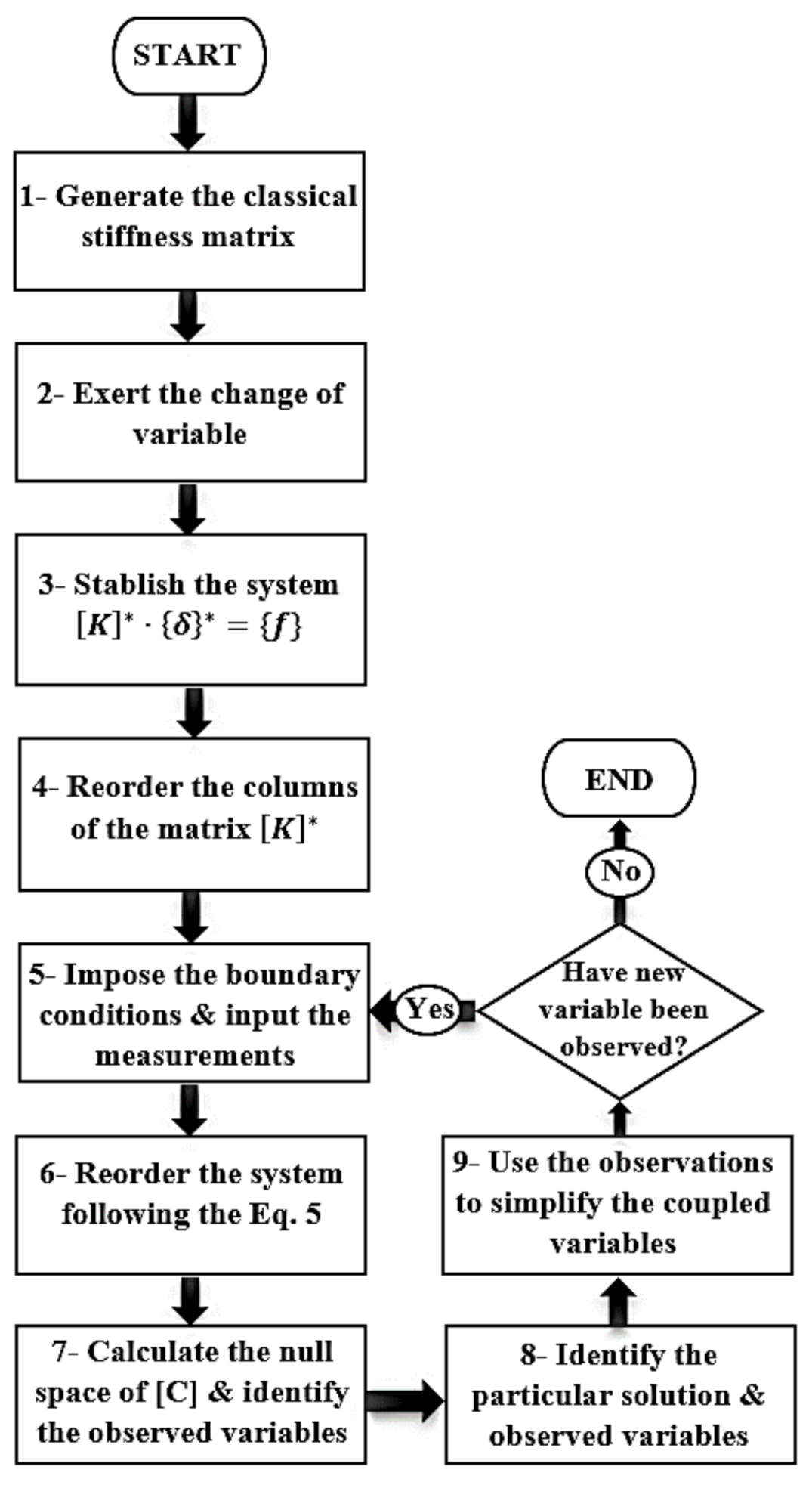
To illustrate the application of the procedure presented above, an algorithm is proposed in this section for the structural system identification of 2D element structures with the OM. This algorithm is presented in Figure 1. The whole package of the 2D observability technique was written in MatLab [40]. This package contains two main connected parts. The first part contains only direct analysis codes. In this part, 2D finite element analyses were developed for the plane strain analysis and the user only needs to input the node coordinates, the mechanical properties, the boundary conditions, and the applied forces. Afterwards, through the interface the user selects the defined structure and runs the direct analysis to calculate the deflections at the free nodes and the reactions at the boundary conditions. Some of the information calculated in this step is used as input data for the inverse analysis of the structure in the second part. The second part of the package was only assigned to inverse analysis and contains the procedure presented in the preceding section. To carry out the inverse analysis, the user has to define the condition of the inverse analysis through the interface. In this step, the interface offers all the possible measurements of the structure calculated in the direct analysis. After selecting the measured degrees of freedom, an observability analysis is performed and the observable variables are provided together with their numerical values. The steps of the algorithm for the inverse analysis of the structure are as follows:

• Step 1. Generate the classical stiffness matrix equation presented in Equation (2).
• Step 2. Exert the change in variable to the stiffness matrix using the functions of Poisson’s ratio presented in Equations (7) and (8).
• Step 3. Establish Equation (3) considering the variables defined in Step 2.
• Step 4. Reorder the columns in matrix to isolate the monomial products of variables.
• Step 5. Introduce the boundary conditions, the known forces, and the measured deflections.
• Step 6. Reorder the system following Equation (5).
• Step 7. Calculate the null space of [C] numerically and identify the observed variables.
• Step 8. Calculate the particular solution of the system numerically using the Moore–Penrose pseudoinverse function.
• Step 9. Use the observed parameters or the observed coupled variables to simplify the other coupled variables.
• Step 10. Introduce the observed parameters into Step 5. Repeat until no additional parameters are observed (end of the recursive process).

A summary of the aforementioned algorithm is illustrated in Figure 1.

2.3. Comparison of the Application of OM to the 1D and 2D Element Structures

To illustrate the effect of changing the type of element into the observability method,

Table 3. Comparison of 1D and 2D observability methods (OMs).

	1D OM	2D OM
		Before Change of Var.	After Change of Var.
Type of element	2-noded beam element	6-noded triangular element	6-noded triangular element
Degrees of freedom per element	6	12	12
Number of unknows	2	2	4
Unknown variables per element	$E_i{A}_i$, $E_i{I}_i$	$E_i$ and ${\vartheta }_i$	$E_i$, ${\vartheta }_i$, $N{U}_i^p$, $N{U}_i^N$
Products of unknowns	($E_i{A}_i$/$L_i) and$ ($E_i{I}_i$/$L_i)$	($E_i{h}_i$/${\vartheta }_i+1$) ($E_i{h}_i$/$2{\vartheta }_i{}^2+{\vartheta }_i-1$), ($E_i{h}_i{\vartheta }_i$/$2{\vartheta }_i{}^2+{\vartheta }_i-1$)	$E_i.h_i.N{U}_i^p$ $E_i.h_i.N{U}_i^p.N{U}_i^N,$ $E_i.h_i.{\vartheta }_i.N{U}_i^p.N{U}_i^N$
Size of stiffness matrix	$\left[3N_N\times 3N_N\right]$	$\left[2N_N\times 2N_N\right]$	$[2N_N\times \left(2N_N\times E_N\times 3\right)$]
Calculation of the null space	Symbolical	Numerical	Numerical

is presented. This table compares the application of 1D (2-noded beam element) and 2D (6-noded triangular element, LST) element structures and includes the following information: (1) type of element, (2) degrees of freedom per element, (3) unknown variables, (4) products of unknown variables, and (5) size of the stiffness matrix and, (6) type of analysis of the null space. The information of the 2D elements is presented before and after the change in variables described in Section 1.

The analysis of Table 3 shows that the number of unknown variables per element is doubled (changing from 2 to 4) after applying the change of variables in the 2D elements. Therefore, the number of columns of the stiffness matrix is also consequently increased. This table also illustrates that, unlike the analysis of 1D elements, a numerical simulation of the null space is required for the analysis of 2D element structures.

3. Example of the Application

In this section, a state-of-the-art example is analyzed to illustrate the applicability of the proposed algorithm to the structural system identification of 2D element structures with observability techniques. Firstly, the geometry, boundary, and loading conditions of the example are detailed together with the results of the direct analysis. Then, some steps of the inverse analysis of the structure are detailed. Finally, a statistical analysis is presented to illustrate the role of the measuring set on the observability of the structural parameters of this structure.

3.1. Definition of the Analyzed Structure

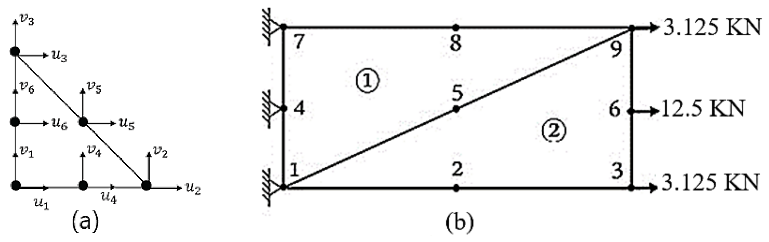
The analyzed structure was chosen from Peter Kattan’s book [45]. This structure corresponds with the discretization of a clamped plate simulated with the plane strain theory. For the finite element model, two quadratic 6-noded LST elements (see Figure 2a) were considered, leading to a system with 9 nodes and 18 degrees of freedom. The boundary and loading conditions as well as the node and element numbering are presented in Figure 2b. The uniform force at the right edge of the structure (corresponding to a distributed load of W = 3000 kN/m²) has been simulated as concentrated forces at the element nodes (nodes 3, 6, and 9), according to the tributary area of each node. As illustrated in this figure, the clamp conditions are modeled by fixing the horizontal and vertical deflections of nodes 1, 4, and 7. The horizontal and vertical deflections of the rest of the nodes in the structure remain free.

The analyzed structure has a length of 0.5 m, a height of 0.25 m, and the thickness of 1 (plane strain assumption). The Young’s modulus and Poisson’s ratio are E = 210 GPa and ϑ = 0.3, respectively. The first part of the developed package was used to calculate the horizontal and vertical deflections at the free nodes as well as the reactions at the boundary conditions (direct analysis). The obtained deflections and reactions are summarized in

Table 4. Deflections and reactions at the example from the direct analysis.

Node	1	2	3	4	5	6	7	8	9
$u_i$(m) e-6		0.080	0.1580		0.0739	0.1568		0.0716	0.1580
$v_i$(m) e-6		0.0227	0.0288		0.0055	0.0113		−0.011	−0.007
$H_i$(KN)	−3.541			−11.67			−3.541
$V_i$(KN)	−2.863			0.012			2.851

. The results obtained from the direct analysis are considered in good agreement with those in [45] (in fact, both results present the same number of decimal numbers).

3.2. Inverse Analysis

In this section, the proposed algorithm is used for the inverse analysis of the structure from the following measurement set (${\mathrm{u}}_2$, ${\mathrm{v}}_2$, ${\mathrm{u}}_3$, ${\mathrm{v}}_3$, ${\mathrm{u}}_5$, ${\mathrm{v}}_5$, ${\mathrm{u}}_6$, ${\mathrm{v}}_6$, ${\mathrm{u}}_9,$ and ${\mathrm{v}}_9$). The numerical values of these deflections correspond with those presented in Table 4.

To identify the observable parameters in the structure, the stiffness matrix system described in Step 1 of the algorithm was calculated. This example contains 18 components for displacements (9 for both u and v). Unfortunately, the large size of this matrix (18 × 18) prevents its representation in the paper and only the first equation (the one related to the horizontal force at node 1, H₁ is depicted) is presented in Equation (10):

$$H_1={\left[\begin{array}{c}((E_1.h_1)/2\left({\vartheta }_1+1\right))+((E_2.h_2)/\left({\vartheta }_2-1\right))/(\left(4.\left(2{\vartheta }_2-1\right).\left({\vartheta }_2+1\right)\right)\\ 0\\ ((E_2.h_2).\left({\vartheta }_2-1\right))/\left(3.\left(2{\vartheta }_2-1\right).\left({\vartheta }_2+1\right)\right)\\ -(2.E_2.h_2.{\vartheta }_2)/\left(3\left(2.{\vartheta }_2-1\right).\left({\vartheta }_2+1\right)\right)\\ (E_2.h_2.\left({\vartheta }_2-1\right))/\left(12\left(2{\vartheta }_2-1\right).\left({\vartheta }_2+1\right)\right)\\ (E_2.h_2.{\vartheta }_2)/6.\left(2{\vartheta }_2-1\right).\left({\vartheta }_2+1\right)\\ -(2.E_1.h_1)/3.\left({\vartheta }_1+1\right)\\ (E_1.h_1)/3.\left({\vartheta }_1+1\right)\\ 0\\ ((2.E_2.h_2.{\vartheta }_2)/\left(3\left(2{\vartheta }_2-1\right).\left({\vartheta }_2+1\right)\right))-((E_1.h_1)/3\left({\vartheta }_1+1)\right)\\ 0\\ 0\\ (E_1.h_1)/(6\left({\vartheta }_1+1\right))\\ -(E_1.h_1)/(12\left({\vartheta }_1+1\right))\\ 0\\ 0\\ 0\\ ((E_1.h_1)/2\left({\vartheta }_1+1\right))-((E_2.h_2.{\vartheta }_2)/\left(6(2{\vartheta }_2-1\right).\left({\vartheta }_2+1\right))\end{array}\right]}^T.\left\{\begin{array}{c}{u}_1\\ v_1\\ u_2\\ v_2\\ u_3\\ v_3\\ u_4\\ v_4\\ u_5\\ v_5\\ u_6\\ v_6\\ u_7\\ v_7\\ u_8\\ v_8\\ u_9\\ v_9\end{array}\right\}$$

(10)

As shown in Equation (10), Poisson’s ratio appears in both the numerator and denominator of the matrix parameters. This location of Poisson’s ratio prevents the application of traditional OM (proposed in the literature) and makes necessary the changes in variables proposed in Step 2. After this change in variables, the system of equations can be rearranged. In this way, the size of the modified stiffness matrix is increased to 18 × 42. Again, for size limitations only the obtained equilibrium equation of H₁ is presented in the paper. This equation is as follows:

$$H_1={\left[\begin{array}{c}0\\ 0\\ 0\\ 0\\ 0\\ -1/3\\ 1/2\\ 0\\ 0\\ -2/3\\ 1/6\\ 2/3\\ 0\\ -1/6\\ 0\\ 0\\ 0\\ 0\\ 0\\ 0\\ 0\\ -1/3\\ 0\\ -1/12\\ -1/3\\ -1/12\\ 0\\ 0\\ 0\\ 0\\ 0\\ 0\\ 0\\ 0\\ 0\\ 0\\ 0\\ 0\\ 0\\ 0\\ 0\\ 0\end{array}\right]}^T. \left\{\begin{array}{c}{E}_1.{\vartheta }_1.N{U}_1^p.N{U}_1^N.u_5\\ E_1.{\vartheta }_1.N{U}_1^p.N{U}_1^N.u_8\\ E_1.{\vartheta }_1.N{U}_1^p.N{U}_1^N.u_9\\ E_1.{\vartheta }_1.N{U}_1^p.N{U}_1^N.v_5\\ E_1.{\vartheta }_1.N{U}_1^p.N{U}_1^N.v_8\\ E_2.{\vartheta }_2.N{U}_2^p.N{U}_2^N.u_2\\ E_2.{\vartheta }_2.N{U}_2^p.N{U}_2^N.u_3\\ E_2.{\vartheta }_2.N{U}_2^p.N{U}_2^N.u_5\\ E_2.{\vartheta }_2.N{U}_2^p.N{U}_2^N.u_6\\ E_2.{\vartheta }_2.N{U}_2^p.N{U}_2^N.v_2\\ E_2.{\vartheta }_2.N{U}_2^p.N{U}_2^N.v_3\\ E_2.{\vartheta }_2.N{U}_2^p.N{U}_2^N.v_5\\ E_2.{\vartheta }_2.N{U}_2^p.N{U}_2^N.v_6\\ E_2.{\vartheta }_2.N{U}_2^p.N{U}_2^N.v_9\\ E_1.N{U}_1^p.N{U}_1^N.u_5\\ E_1.N{U}_1^p.N{U}_1^N.u_8\\ E_1.N{U}_1^p.N{U}_1^N.u_9\\ E_1.N{U}_1^p.N{U}_1^N.v_5\\ E_1.N{U}_1^p.N{U}_1^N.v_8\\ E_1.N{U}_1^p.u_5\\ E_1.N{U}_1^p.u_8\\ E_1.N{U}_1^p.v_5\\ E_1.N{U}_1^p.v_8\\ E_1.N{U}_1^p.v_9\\ E_2.N{U}_2^p.N{U}_2^N.u_2\\ E_2.N{U}_2^p.N{U}_2^N.u_3\\ E_2.N{U}_2^p.N{U}_2^N.u_5\\ E_2.N{U}_2^p.N{U}_2^N.u_6\\ E_2.N{U}_2^p.N{U}_2^N.v_2\\ E_2.N{U}_2^p.N{U}_2^N.v_3\\ E_2.N{U}_2^p.N{U}_2^N.v_5\\ E_2.N{U}_2^p.N{U}_2^N.v_6\\ E_2.N{U}_2^p.N{U}_2^N.v_9\\ E_2.N{U}_2^p.u_2\\ E_2.N{U}_2^p.u_3\\ E_2.N{U}_2^p.u_5\\ E_2.N{U}_2^p.u_6\\ E_2.N{U}_2^p.u_9\\ E_2.N{U}_2^p.v_2\\ E_2.N{U}_2^p.v_3\\ E_2.N{U}_2^p.v_5\\ E_2.N{U}_2^p.v_6\end{array}\right\}$$

(11)

After introducing the known information (null deflections at the boundary conditions; deflections at the measurement set; and known forces at nodes 3, 6 and 9), the system of equations was arranged as presented in Step 6. To proceed this application, the equilibrium equation of the horizontal reaction at node 2, H₂, is presented. This equation is as follows:

$$H_2={\left[\begin{array}{c}0\\ 0\\ 0\\ 2\times {10}^{-07}\\ 0\\ 0\\ 0\\ 0\\ 0\\ 0\\ 9\times {10}^{-08}\\ 9\times {10}^{-08}\\ 0\\ 0\\ 0\\ 0\\ 0\\ 0\end{array}\right]}^T.\left\{\begin{array}{c}{E}_1.{\vartheta }_1.N{U}_1^p.N{U}_1^N\\ E_1.{\vartheta }_1.N{U}_1^p.N{U}_1^N.u_8\\ E_1.{\vartheta }_1.N{U}_1^p.N{U}_1^N.v_8\\ E_2.{\vartheta }_2.N{U}_2^p.N{U}_2^N\\ E_1.N{U}_1^p\\ E_1.N{U}_1^p.N{U}_1^N\\ E_1.N{U}_1^p.N{U}_1^N.u_8\\ E_1.N{U}_1^p.N{U}_1^N.v_8\\ E_1.N{U}_1^p.u_8\\ E_1.N{U}_1^p.v_8\\ E_2.N{U}_2^p\\ E_2.N{U}_2^p.N{U}_2^N\\ H_1\\ H_4\\ H_7\\ V_1\\ V_4\\ V_7\end{array}\right\}$$

(12)

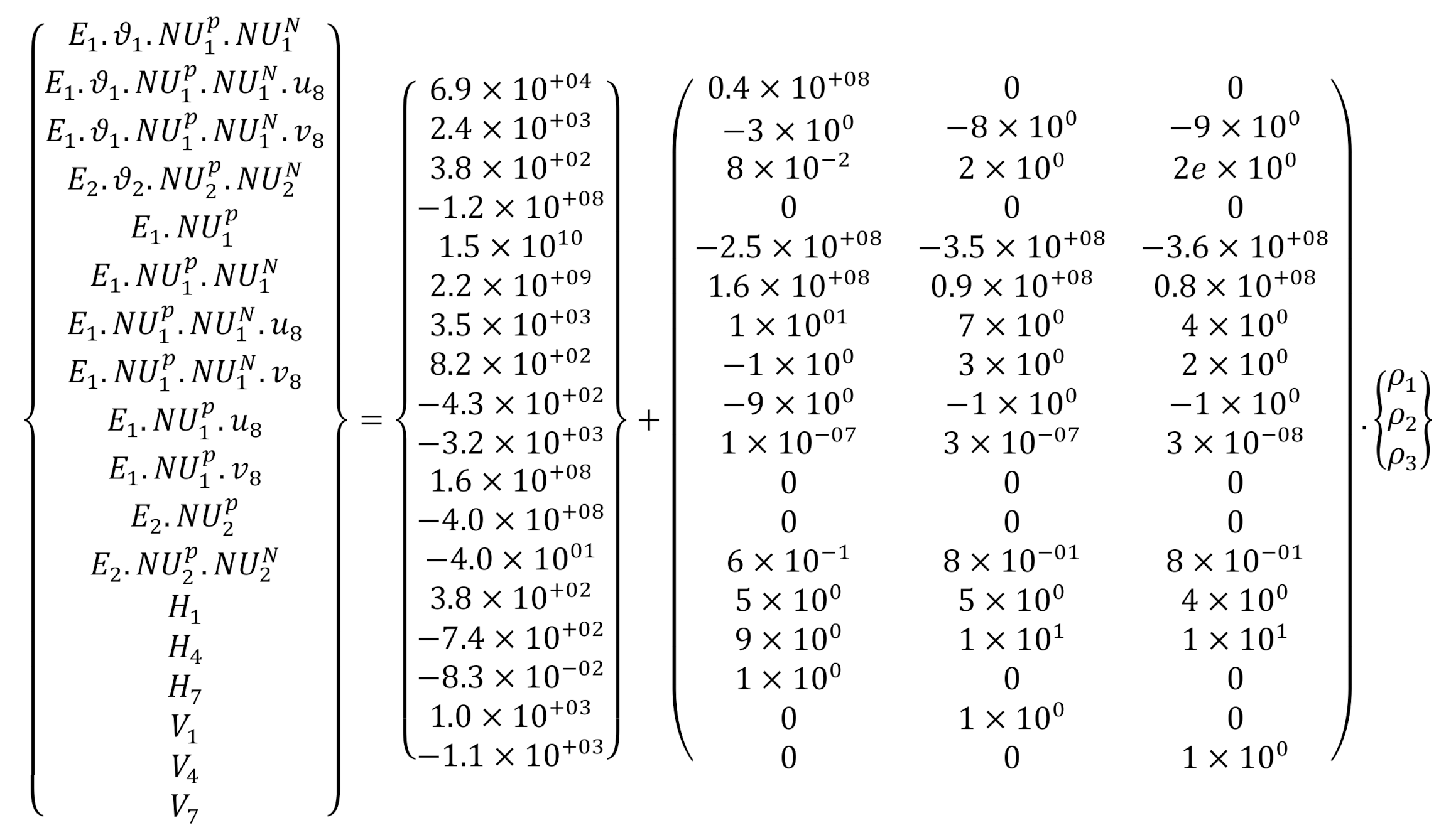
This equation shows that at this stage, the number of unknown variables in the system is eight (${\mathrm{E}}_1$, ${\vartheta }_1$, ${\mathrm{NU}}_1^{\mathrm{p}}$, ${\mathrm{NU}}_1^{\mathrm{N}}$, ${\mathrm{E}}_2$, ${\vartheta }_2$, ${\mathrm{NU}}_2^{\mathrm{p}}$, ${\mathrm{NU}}_2^{\mathrm{N}}$). To identify the observability of the variables, the null space [V] was numerically calculated in Step 7. With this information, the general solution of the system {z} described in Equation (6) can be written as presented in Figure 3.

The analysis of the null space presented in Figure 3 shows that the partial observability of the structure is obtained. The particular solution of these parameters was numerically obtained with the pseudoinverse of matrix [C] in MatLab (Step 8). In Figure 3, the observable parameters (the ones with a unique solution) are associated with the null rows of the matrix [V]. The values of these parameters are $({\vartheta }_2.{\mathrm{E}}_2.{\mathrm{NU}}_2^{\mathrm{p}}.{\mathrm{NU}}_2^{\mathrm{N}})= -1.2\times {10}^{+08}$, $({\mathrm{E}}_2.{\mathrm{NU}}_2^{\mathrm{p}}$.${ \mathrm{NU}}_2^{\mathrm{N}})$= $-4.0\times {10}^{+08}$, and $({\mathrm{E}}_2.{\mathrm{NU}}_2^{\mathrm{P}})$= $1.6\times {10}^{+08}$. Finally, by dividing the observable coupled variables to each other, the following results were obtained for element 2 of the structure: ${\mathrm{NU}}_2^{\mathrm{P}}$= $7.7\times {10}^{-01}$, ${\mathrm{NU}}_2^{\mathrm{N}}$= $-25\times {10}^{-1}$, ${\mathrm{E}}_2$= $2.1\times {10}^{+08}$ Pa, and ${\vartheta }_2$= $3\times {10}^{-01}$ Increasing the number of measurements may lead to increasing the number of observed parameters or full observability. To illustrate the effect of the number of measurements on the observability of the system, a statistical analysis is presented in the following section.

3.3. Statistical Analysis

In this part, a statistical analysis of the example is presented to indicate the required number of measurements for the partial and full observability of the system. To do so, combinatorial analysis was conducted and the following combinatory equation was used:

$$\mathrm{C}\left(\mathrm{n},\mathrm{r}\right)=\left(\mathrm{n}!\right)/\left(\mathrm{r}!\left(\mathrm{n}-\mathrm{r}\right)!\right),$$

(13)

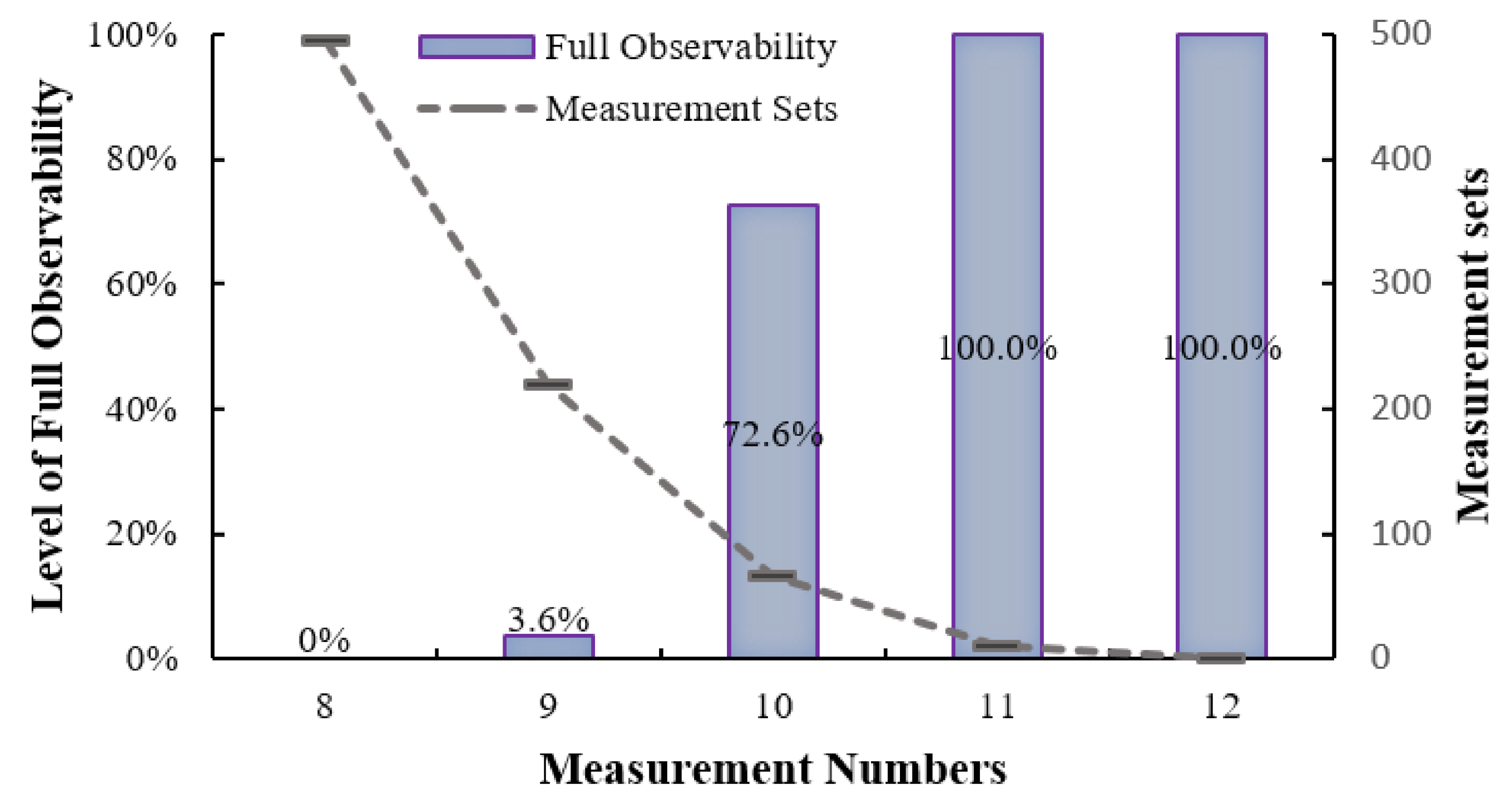
with n as the number of possible measurement and r as the chosen number of measurements in each combination. In the analyzed example, n is equal to 12, as the possible measurements correspond to $u_2$, $v_2$, $u_3$, $v_3$, $u_5$, $v_5$, $u_6$, $v_6$, $u_8$, $v_8$, $u_9,$ and $v_9$. This combinatorial analysis was carried out for 8 (${\mathrm{C}}_{12}^8=495$), 9 (${\mathrm{C}}_{12}^9=220$), 10 (${\mathrm{C}}_{12}^{10}=66$), 11 (${\mathrm{C}}_{12}^{11}=12$), and 12 (${\mathrm{C}}_{12}^{12}=1$) measurements per set. It can be seen in Figure 4 that the full observability of the structure requires at least nine measurements per set. In the case of eight measurements, 0.6% of the sets lead to the partial observability of the system, and 99.4% lead to an indeterminate system. For the case of nine measurements, 3.6% lead to the full observability of the system, 4.6% of the sets lead to the partial observability of the system, and 91.8% lead to an indeterminate system. This figure also shows that by conducting 10 measurements, 72.6% of the measurements lead to the full observability of the system, 1.5% of the sets lead to the partial observability of the system, and 25.9% lead to an indeterminate system.

As illustrated in

Table 5. All the sets for achieving different levels of observability for 8, 9, and 10 measurements per set. Partial observability (P.O.) and full observability (F.O.).

8 Measurements	9 Measurements		10 Measurements
P.O.	F.O.	P.O.	F.O.	P.O.
2,$\overline{3}$,$\overline{5}$,$\overline{6}$,9	$2,\overline{3},\overline{5}$$, \overline{6}$,8,9	$2,\overline{3},\overline{5}$$, \overline{6}$$, \overline{9}$	$\overline{3}$,$\overline{5}$,$\overline{6}$,$\overline{8}$,$\overline{9}$	$\overline{2}$,$\overline{3}$,$\overline{5}$,$\overline{6}$,$\overline{9}$
$\overline{2}$,$\overline{3}$,$\overline{5}$,6,9	$2,\overline{5}$$, \overline{6}$$, \overline{8}$$, \overline{9}$	$\overline{2},3,\overline{5}$$, \overline{6}$$, \overline{9}$	2,3,$\overline{5}$,$\overline{6}$,$\overline{8}$,$\overline{9}$
$\overline{2}$,$\overline{3}$,$\overline{5}$,$\overline{6}$	$\overline{2}$$, \overline{3}$$, \overline{5}$,6,8,9	$\overline{2},\overline{3},5$$,\overline{6}$$,\overline{9}$	2,$\overline{3}$,$\overline{5},$6,$\overline{8}$,$\overline{9}$
	$\overline{2}$$, \overline{3}$$, \overline{5}$$, \overline{6}$,8	$\overline{2}$$, \overline{3}$$, \overline{5}$$,6,\overline{9}$	2,$\overline{3}$,$\overline{5}$,$\overline{6}$,8,$\overline{9}$
		$\overline{2}$$, \overline{3}$$, \overline{5}$$,\overline{6}$,9	2,$\overline{3}$,$\overline{5}$,$\overline{6}$,$\overline{8}$,9
			$\overline{2}$$, \overline{5}$$, \overline{6}$$, \overline{8}$$, \overline{9}$
			$\overline{2}$$,$$,6,\overline{8}$$, \overline{9}$
			$\overline{2}$$,3, \overline{5},\overline{6}$$,8, \overline{9}$
			$\overline{2}$$,3, \overline{5}$$, \overline{6}$$, \overline{8}$,9
			$\overline{2}$,$\overline{3}$,5,$\overline{6}$,8,$\overline{9}$
			$\overline{2}$,$\overline{3}$,$\overline{5},\overline{8}$,$\overline{9}$
			$\overline{2}$,$\overline{3}$,$\overline{5},6,8, \overline{9}$
			$\overline{2}$,$\overline{3}$, $\overline{5}$,6,$\overline{8}$,9
			$\overline{2}$,$\overline{3}$,$\overline{5}$,$\overline{6}$,$\overline{8}$

, to distinguish the difference between the sets achieving different levels of observability, they were classified into different patterns with regard to the location of the measurements. For instance, in the case of eight measurements $\left\{\mathrm{u}|{\mathrm{v}}_2,{\mathrm{u}}_3,{\mathrm{v}}_3,{\mathrm{u}}_5,{\mathrm{v}}_5,{\mathrm{u}}_6,{\mathrm{v}}_6,\mathrm{u}|{\mathrm{v}}_9\right\}$, $\left\{{\mathrm{u}}_2,{\mathrm{v}}_2,{\mathrm{u}}_3,{\mathrm{v}}_3,{\mathrm{u}}_5,{\mathrm{v}}_5,\mathrm{u}|{\mathrm{v}}_6, \mathrm{u}|{\mathrm{v}}_9\right\}$, and $\left\{{\mathrm{u}}_2,{\mathrm{v}}_2,{\mathrm{u}}_3,{\mathrm{v}}_3,{\mathrm{u}}_5,{\mathrm{v}}_5,{\mathrm{u}}_6,{\mathrm{v}}_6\right\}$ were classified as $\left\{2, \overline{3}, \overline{5}, \overline{6},9\right\}$, $\left\{\overline{2}, \overline{3}, \overline{5},6,9\right\}$, and $\{\overline{2}$,$\overline{3}$,$\overline{5}$,$\overline{6}\}$, respectively (the vertical bar between u and v indicates that either the vertical or horizontal degree of freedom is measured). In these patterns, the subscripts of the measurements (node number) that identify the associated location are shown.

The node numbers with the sign ($-$) indicate that both deflections, vertical and horizontal, are measurements. However, no distinction is made between the measurements of X and Y degrees of freedom, as the ones without any sign are indicative of either vertical or horizontal measurements. All the sets related to the PO of the system in the cases of 8, 9, and 10 measurements are listed in columns 1, 3, and 5 of Table 5, respectively. However, columns 2 and 4 include the sets for FO of the system based on 9 and 10 measurements. One of the surprising results of the method is that, with eight targeted unknowns, at least nine measurements are required to obtain full observability. This is one of the drawbacks inherent in the method. As the nonlinear problem is being solved as a linear one and coupled unknowns are linearized, extra information might be required to uncouple them and to obtain full observability.

It is clear that no set with 8, 9, or 10 measurements leads to the FO of the examined structure. Hence, if those are not elected appropriately, the end of the recursive process occurs before identifying all variables. In Table 5, the sets leading to the FO of the system are selected at dispersed locations of the structure. With these sets, in the other words, the distributed placement of the sensors keeps the observability flow, and, consequently, FO will be obtained. If the measurements are conducted intensively at a local area or specific element of the structure, the redundancy of the measurements will emerge.

In the same manner, in the case of $\left\{2,\overline{3},\overline{5}, \overline{6},8,9\right\}$ (the first set related with nine measurements), achieving the FO was due to the dispersed locations of the sensors at all nodes of the structure. Accordingly, for the same number of measurements as well as 10, the occurrence of PO in all sets (third and fifth columns of Table 5) is due to a lack of any information about node 8. For instance, choosing the measurement set, $\{\overline{2}$,$\overline{3}$,$\overline{5}$,$\overline{6}$,$\overline{9}\}$ leads to partial observability despite 10 measurements being included in the set.

This set will only allow a unique solution for the following coupled unknowns $\left\{E_2.{\vartheta }_2.N{U}_2^p.N{U}_2^N\right\}$, $\left\{E_2.N{U}_2^p.N{U}_2^N\right\}$, and $\left\{E_2.N{U}_2^p\right\}$. However, the first set in the fourth column of Table 5, $\{\overline{3}$,$\overline{5}$,$\overline{6}$,$\overline{8}$,$\overline{9}\},$ without any information about node 2 enabled the FO of the system. In the first recursive step of the inverse analysis, the particular solutions for the couple $\left\{E_1.N{U}_1^p.N{U}_1^N\right\}$ and $\left\{E_1.N{U}_1^p\right\}$ related to element 1 as well as $\left\{E_2.{\vartheta }_2.N{U}_2^p.N{U}_2^N\right\}$ and $\left\{E_2.N{U}_2^p.N{U}_2^N\right\}$ related to element 2 are acquired. This information is sufficient to derive the value of the parameters $N{U}_1^N$ and ${\vartheta }_2$ first and the rest of unknowns of the system. All the above information implies that the reason for the partial observability is that the number of effective measurements is less than the number of unknowns.

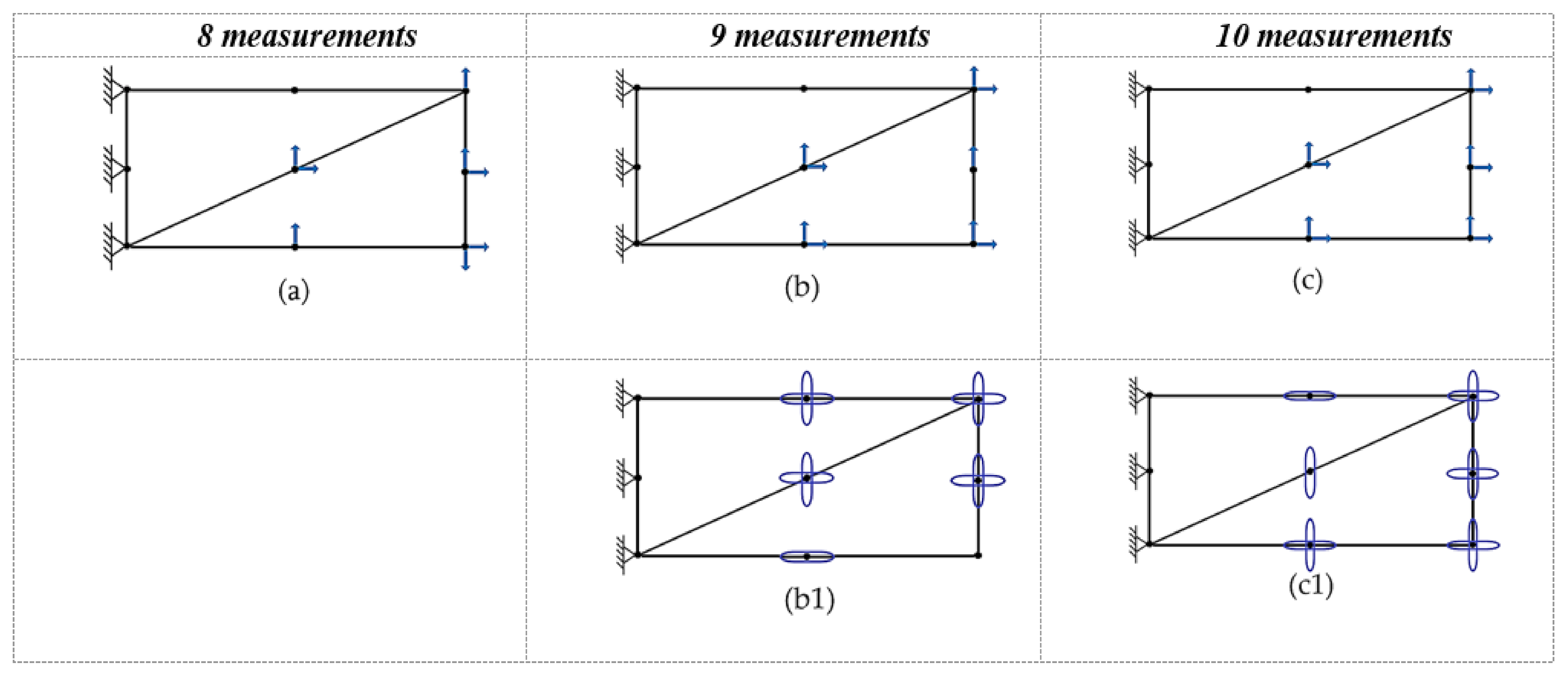
Figure 5 illustrates some of the mentioned possible sets (in Table 5) containing both vertical and horizontal measurements. Figure 5a–c presents the sets that lead to the PO of the system by measuring 8, 9, and 10 deflections, respectively. The FO of the problem through 9 and 10 measurements is depicted in Figure 5b1,c1, respectively.

4. Conclusions

The observability technique has been studied in the literature for the structural system identification of 1D element structures (such as beams and trusses). Nevertheless, the application of this method to 2D element structures (such as dams, tunnels, and culverts) has not been studied yet. Despite how it may appear, this application is not straightforward, as the unknown variables in the system are not only located in the numerator. In fact, the location of these variables also in the denominator makes the system of equations nonlinear and prevents the application of traditional observability techniques for this type of structure. To fill this gap, an algorithm for the observability analysis of 2D element structures was developed in this paper. The main contribution of this algorithm refers to the development of a new change in variables to linearize the system of equations and makes OM applicable for 2D element structures. The proposed methodology is characterized by its generality, as similar changes in variables can be used to linearize other nonlinear problems when the unknown variables appear in both the numerator and denominator of the system of equations.

To illustrate the applicability of the proposed algorithm, a state-of-the-art example (cantilever plate) was analyzed with the plane strain theory. This analysis included a step-by-step mathematical review of the system of equations, as well as a statistical study of the structural system identification with different measurement sets. The obtained results show that the unknown parameters (such as the Young’s Modulus, E, and Poisson’s Ratio, v) are successfully calculated with the proposed methodology.

References

- Ceravolo, R.; Faraci, A.; Miraglia, G. Bayesian Calibration of Hysteretic Parameters with Consideration of the Model Discrepancy for Use in Seismic Structural Health Monitoring. Appl. Sci. 2020, 10, 5813. [Google Scholar] [CrossRef]
- Park, J. Special feature vibration-based structural health monitoring. Appl. Sci. 2020, 10, 5139. [Google Scholar] [CrossRef]
- Sirca, G.F.; Adeli, H. System identification in structural engineering. Sci. Iran. 2012, 19, 1355–1364. [Google Scholar] [CrossRef] [Green Version]
- Liu, H.; Wang, X.; Tan, G.; He, X.; Luo, G. System reliability evaluation of prefabricated RC hollow slab bridges considering hinge joint damage based on modified AHP. Appl. Sci. 2019, 9, 4841. [Google Scholar] [CrossRef] [Green Version]
- Campos, J.; Sharma, P.; Albano, M.; Ferreira, L.; Larrañaga, M. An Open Source Framework Approach to Support Condition Monitoring and Maintenance. Appl. Sci. 2020, 10, 6360. [Google Scholar] [CrossRef]
- Romero, F.; Lofrano, E.; Paolone, A. Damage identification in parabolic arc via orthogonal empirical mode decomposition. In Proceedings of the International Design Engineering Technical Conference and Computers and Information in Engineering, Buffalo, NY, USA, 17–20 August 2014. [Google Scholar] [CrossRef]
- Lofrano, E.; Romero, M.; Paolone, A. A pseudo-model structural damage index based on orthogonal empirical mode decomposition. J. Mech. Sci. 2019. [Google Scholar] [CrossRef]
- Wu, Z.; Liu, G.; Zhang, Z. Experimental study of structural damage identification based on modal parameters and decay ratio of acceleration signals. Front. Archit. Civ. Eng. China 2011, 5, 112–120. [Google Scholar] [CrossRef]
- Salavati, M. Approximation of structural damping and input excitation force. Front. Struct. Civ. Eng. 2017, 11, 244–254. [Google Scholar] [CrossRef]
- Xia, Y.; Lei, X.; Wang, P.; Liu, G.; Sun, L. Long-term performance monitoring and assessment of concrete beam bridges using neutral axis indicator. Struct. Control Health Monit. 2020, 27, e2637. [Google Scholar] [CrossRef]
- Zhao, C.; Lavasan, A.A.; Barciaga, T.; Zarev, V.; Datcheva, M.; Schanz, T. Model validation and calibration via back analysis for mechanized tunnel simulations—The Western Scheldt tunnel case. Comput. Geotech. 2015, 69, 601–614. [Google Scholar] [CrossRef]
- Xia, Y.; Wang, P.; Sun, L. Neutral Axis Position Based Health Monitoring and Condition Assessment Techniques for Concrete Box Girder Bridges. Int. J. Struct. Stab. Dyn. 2019, 19, 1940015. [Google Scholar] [CrossRef]
- Yassine, R.; Salman, F.; Shaer, A.; Hammad, M.; Duhamel, D. Application of the recursive finite element approach on 2D periodic structures under harmonic vibration. Computation 2017, 5, 1. [Google Scholar] [CrossRef] [Green Version]
- Hashash, Y.M.A.; Levasseur, S.; Osouli, A.; Finno, R.; Malecot, Y. Comparison of two inverse analysis techniques for learning deep excavation response. Comput. Geotech. 2010, 37, 323–333. [Google Scholar] [CrossRef]
- Dudley, D.G.; Pao, H.Y. System identification for wireless propagation channels in tunnels. IEEE Trans. Antennas Propag. 2005, 53, 2400–2405. [Google Scholar] [CrossRef]
- Sakurai, S.; Akutagawa, S.; Takeuchi, K.; Shinji, M.; Shimizu, N. Back analysis for tunnel engineering as a modern observational method. Tunn. Undergr. Sp. Technol. 2003, 18, 185–196. [Google Scholar] [CrossRef]
- Sakurai, S.; Takeuchi, K. Back analysis of measured displacements of tunnels. Rock Mech. Rock Eng. 1983, 16, 173–180. [Google Scholar] [CrossRef]
- Bhalla, S.; Yang, Y.W.; Zhao, J.; Soh, C.K. Structural health monitoring of underground facilities—Technological issues and challenges. Tunn. Undergr. Sp. Technol. 2005, 20, 487–500. [Google Scholar] [CrossRef]
- Mobaraki, B.; Vaghefi, M. Effect of the soil type on the dynamic response of a tunnel under surface detonation. Combust. Explos. Shock Waves 2016, 52, 363–370. [Google Scholar] [CrossRef]
- Mobaraki, B.; Vaghefi, M. Numerical study of the depth and cross-sectional shape of tunnel under surface explosion. Tunn. Undergr. Sp. Technol. 2015, 47, 114–122. [Google Scholar] [CrossRef]
- Khamesi, H.; Torabi, S.R.; Mirzaei-Nasirabad, H.; Ghadiri, Z. Improving the Performance of Intelligent Back Analysis for Tunneling Using Optimized Fuzzy Systems: Case Study of the Karaj Subway Line 2 in Iran. J. Comput. Civ. Eng. 2014, 29, 05014010. [Google Scholar] [CrossRef]
- Dehghan, A.N.; Shafiee, S.M.; Rezaei, F. 3-D stability analysis and design of the primary support of Karaj metro Tunnel: Based on convergence data and back analysis algorithm. Eng. Geol. 2012, 141, 141–149. [Google Scholar] [CrossRef]
- Germoso, C.; Quaranta, G.; Duval, J.L.; Chinesta, F. Non-instrusive in-plane-out-of-plane seperated representation in 3D parametric elastodynamics. Computation 2020, 8, 78. [Google Scholar] [CrossRef]
- Xia, Y.; Jian, X.; Yan, B.; Su, D. Infrastructure Safety Oriented Traffic Load Monitoring Using Multi-Sensor and Single Camera for Short and Medium Span Bridges. Remote Sens. 2019, 11, 2651. [Google Scholar] [CrossRef] [Green Version]
- Vardakos, S.; Gutierrez, M.; Xia, C. Parameter identification in numerical modeling of tunneling using the Differential Evolution Genetic Algorithm (DEGA). Tunn. Undergr. Sp. Technol. 2012, 28, 109–123. [Google Scholar] [CrossRef]
- Xiang, Z.; Swoboda, G.; Cen, Z. Optimal Layout of Displacement Measurements for Parameter Identification Process in Geomechanics. Int. J. Geomech. 2003, 3, 205–216. [Google Scholar] [CrossRef]
- Santos, C.; Ledesma, A.; Gens, A. Backanalysis of measured movements in ageing tunnels. In Geotechnical Aspects of Underground Construction in Soft Ground; CRC Press: Boca Raton, FL, USA, 2012; pp. 223–229. [Google Scholar]
- Lozano-Galant, J.A.; Nogal, M.; Castillo, E.; Turmo, J. Application of observability techniques to structural system identification. Comput. Civ. Infrastruct. Eng. 2013, 28, 434–450. [Google Scholar] [CrossRef]
- Lozano-Galant, J.A.; Nogal, M.; Paya-Zaforteza, I.; Turmo, J. Structural system identification of cable-stayed bridges with observability techniques. Struct. Infrastruct. Eng. 2014, 10, 1331–1344. [Google Scholar] [CrossRef]
- Castillo, E.; Lozano-Galant, J.A.; Nogal, M.; Turmo, J. New tool to help decision making in civil engineering. J. Civ. Eng. Manag. 2015, 21, 689–697. [Google Scholar] [CrossRef] [Green Version]
- Nogal, M.; Lozano-Galant, J.A.; Turmo, J.; Castillo, E. Numerical damage identification of structures by observability techniques based on static loading tests. Struct. Infrastruct. Eng. 2016, 12, 1216–1227. [Google Scholar] [CrossRef] [Green Version]
- Lei, J.; Nogal, M.; Lozano-Galant, J.A.; Xu, D.; Turmo, J. Constrained observability method in static structural system identification. Struct. Control Health Monit. 2018, 25, 1–15. [Google Scholar] [CrossRef]
- Lei, J.; Xu, D.; Turmo, J. Static structural system identification for beam-like structures using compatibility conditions. Struct. Control Health Monit. 2017, 25, 1–15. [Google Scholar] [CrossRef] [Green Version]
- Lozano-Galant, J.A.; Nogal, M.; Turmo, J.; Castillo, E. Selection of measurement sets in static structural identification of bridges using observability trees. Comput. Concr. 2015, 15, 771–794. [Google Scholar] [CrossRef]
- Tomàs, D.; Lozano-Galant, J.A.; Ramos, G.; Turmo, J. Structural system identification of thin web bridges by observability techniques considering shear deformation. Thin-Walled Struct. 2018, 123, 282–293. [Google Scholar] [CrossRef] [Green Version]
- Emadi, S.; Lozano-Galant, J.A.; Xia, Y.; Ramos, G.; Turmo, J. Structural system identification including shear deformation of composite bridges from vertical deflection. Steel Compos. Struct. 2019, 32, 731–741. [Google Scholar] [CrossRef]
- Peng, T.; Casas, J.R.; Lozano-Galant, J.A.; Turmo, T. Constrained observability techniques for structural system identification using modal analysis. J. Sound Vib. 2020, 479. [Google Scholar] [CrossRef]
- Rao, S.S. Analysis of plates. In The Finite Element Method in Engineering, 6th ed.; Elsevier: Amsterdam, The Netherlands, 2018; pp. 379–425. [Google Scholar] [CrossRef]
- Castillo, E.; Nogal, M.; Lozano-Galant, J.A.; Turmo, J. Solving Some Special Cases of Monomial Ratio Equations Appearing Frequently in Physical and Engineering Problems. Math. Probl. Eng. 2016, 2016, 1–29. [Google Scholar] [CrossRef]
- MathWorks. MATLAB; The MathWorks, Inc.: Natick, MA, USA, 2018. [Google Scholar]
- Ramesh, S.S.; Wang, C.M.; Reddy, J.N.; Ang, K.K. Computation of stress resultants in plate bending problems using higher-order triangular elements. Eng. Struct. 2008, 30, 2687–2706. [Google Scholar] [CrossRef]
- Yang, Y.; Tang, X.; Zheng, H. A three-node triangular element with continuous nodal stress. Comput. Struct. 2014, 141, 46–58. [Google Scholar] [CrossRef]
- Piltner, R.; Taylor, R.L. Triangular finite elements with rotational degrees of freedom and enhanced strain modes. Comput. Struct. 2000, 75, 361–368. [Google Scholar] [CrossRef]
- Neto, M.A.; Leal, R.P.; Yu, W. A triangular finite element with drilling degrees of freedom for static and dynamic analysis of smart laminated structures. Comput. Struct. 2012, 108, 61–74. [Google Scholar] [CrossRef]
- Kattan, P.I. MATLAB Guide to Finite Elements; Springer: Berlin/Heidelberg, Germany, 2014. [Google Scholar] [CrossRef]
Figure 1.
Flow chart of the algorithm.
Figure 2.
Example: (a) 6-noded triangular element (LST), and (b) node and element numbering together with the boundary and loading conditions [45].
Figure 3.
General solution of the system of equation.
Figure 4.
Full observability of the system based on the various measurement sets.
Figure 5.
Required number of measurements for having the partial (a,b,c) and full observability (b1,c1) of the system.