
Fake It Till You Make It: Guidelines for Effective Synthetic Data Generation

Department of Information Systems and Security, College of IT, United Arab Emirates University, Al Ain 15551, United Arab Emirates
*
Author to whom correspondence should be addressed.
Appl. Sci. 2021, 11(5), 2158; https://0-doi-org.brum.beds.ac.uk/10.3390/app11052158
Submission received: 31 January 2021
/
Revised: 22 February 2021
/
Accepted: 24 February 2021
/
Published: 28 February 2021
(This article belongs to the Special Issue Generative Models in Artificial Intelligence and Their Applications)
Abstract
:Synthetic data provides a privacy protecting mechanism for the broad usage and sharing of healthcare data for secondary purposes. It is considered a safe approach for the sharing of sensitive data as it generates an artificial dataset that contains no identifiable information. Synthetic data is increasing in popularity with multiple synthetic data generators developed in the past decade, yet its utility is still a subject of research. This paper is concerned with evaluating the effect of various synthetic data generation and usage settings on the utility of the generated synthetic data and its derived models. Specifically, we investigate (i) the effect of data pre-processing on the utility of the synthetic data generated, (ii) whether tuning should be applied to the synthetic datasets when generating supervised machine learning models, and (iii) whether sharing preliminary machine learning results can improve the synthetic data models. Lastly, (iv) we investigate whether one utility measure (Propensity score) can predict the accuracy of the machine learning models generated from the synthetic data when employed in real life. We use two popular measures of synthetic data utility, propensity score and classification accuracy, to compare the different settings. We adopt a recent mechanism for the calculation of propensity, which looks carefully into the choice of model for the propensity score calculation. Accordingly, this paper takes a new direction with investigating the effect of various data generation and usage settings on the quality of the generated data and its ensuing models. The goal is to inform on the best strategies to follow when generating and using synthetic data.
1. Introduction
1.1. Background
Big data is profoundly changing the way organizations perform their businesses. Examples of big data applications include enhanced business intelligence, personalized marketing and cost reduction planning. The possibilities are endless as the availability of massive data is inspiring people to explore many different and life changing applications. One of the most promising fields where big data can be applied to make a change is healthcare [1]. The application of machine learning to health data has the potential to predict and better tackle epidemics, improve quality of care, reduce healthcare costs and advance personalized treatments [2,3,4]. Yet, these improvements are not yet fully realized. The main reason is the limited access to health data due to valid privacy concerns. In fact, releasing and sharing health data entails the risk of compromising the confidentiality of sensitive information and the privacy of the involved individuals [5]. It is governed by ethical and legal standards such as the EU’s General Directive on Data Protection GDPR and the Health Insurance Portability and Accountability Act privacy rule of the U.S. (HIPAA privacy rule) [6,7]. Under these regulations, it is very hard to share high quality data with analysts without informed consent from the data subjects [8]. In fact, many projects are discarded before they begin due to delays to acquire data [9]. Typically, 18 months is the average timeframe to establish a data sharing agreement [10].
Anonymization is another approach for addressing privacy legislations [11,12,13], it is defined as a “technique to prevent identification taking into account all the means reasonably likely to be used to identify a natural person” [6,14]. It is a process of information sanitization that produces data that cannot be linked back to its originators. However, the effectiveness of anonymization has been called into question as the possibility of re-identification through demographic, clinical, and genomic data has been demonstrated in various circumstances [15,16].
An increasingly popular way to overcome the issues of data availability is to use fully synthetic data. Fully Synthetic data generates an artificial dataset that contains no identifiable information about the dataset it was generated from and is considered a safe approach for the sharing of sensitive data [17,18]. It was proposed by Rubin in 1993 to solve the issues of privacy and availability [19]. It has been argued that fully synthetic data does not carry privacy risks as it does not map to real individuals [18,20,21]. The application of Synthetic data to the healthcare domain is recent yet increasing in popularity. The recent 2020 future of privacy forum, cited synthetic data generation as a crucial privacy enhancing technology for the coming decade [22].
Research in the synthetic data domain is thriving in two main directions: (i) some investigators are designing new synthetic data generation mechanisms [23,24,25,26], while (ii) others are exploring the efficiency of such generators in real-life scenarios [27,28,29,30,31,32,33]. In this paper, we take a new and essential direction into investigating the effect of various data generation and usage settings on the quality of the generated data and its ensuing models. The goal is to inform on the best strategies to follow when generating and using synthetic data.
1.2. Contributions
Synthetic data is often generated from original raw (non-processed) data as it is widely believed that “data must be modeled in its original form” [23], prior to the application of any transformations, and that missing values should be represented as they provide information about the dataset [23,24,29]. While this seems like a reasonable assumption, it has not been empirically tested on real data. On the other hand, the effect of different machine learning settings on the utility of the models generated from synthetic data have not been tested/discussed in the literature. Indeed, there are no recommendations on how best to use the generated synthetic data in real life scenarios, and how to set the different parameters of the machine learning models. Lastly, when comparing different data synthesis mechanisms, different data utility measures are used across the literature. There exists no standard mechanism/measure for synthetic data utility, instead, multiple measures have been defined and used across the literature, with emphasis on classification accuracy and propensity score [10,23,24,27,28,29,30,34].
In this paper we try to tackle some of these issues by performing an empirical investigation on synthetic data generated from four well-known synthetic data generators: Synthetic Data Vault, Data Synthesizer, Synthpop parametric and non-parametric [23,24,25,26]. In particular, (i) we investigate the effect of data pre-processing on the utility of the synthetic data generation process, (ii) we also investigate whether parameter tuning (and feature selection) should be applied to the synthetic datasets when generating supervised machine learning models, and whether (iii) sharing preliminary machine learning results (along with the synthetic data) can improve the synthetic data models. Lastly, (iv) we investigate whether propensity is a good predictor for classification accuracy. The purpose of this investigation is to guide practitioners on the best strategies to adopt when working with synthetic data.
The paper is organized as follows: In the next section, we present the four publicly available synthetic data generation techniques that are based on well-known and influential work in this area [10,23,24,29], we also present two predominant synthetic data utility measures, propensity score and classification accuracy [25,27,28,29,30]. In Section 3, we present our empirical methods for the evaluation of various synthetic data generation and usage settings. Section 4 presents the experiments performed and discusses the results. The paper is then completed with a summary of the results along with concluding remarks and limitations.
2. Methods: Synthetic Data Generation and Utility
Synthetic datasets are generated from a model that is fit to a real data set. First the model is constructed then the model is used to produce the synthetic data. Such production process is stochastic, implying that the model produces a different synthetic dataset every time.
Formally, the data synthesis problem can be described as follows: given a private dataset containing individuals extracted from a population of individuals (for example the Canadian population). Each row is an individual’s record containing numerical or categorical attributes (such as demographics, dates, sensitive attributes) taking values from a space . The goal of synthetic data generators is to take this private dataset as input, and construct a statistical model that captures the statistical properties of the population , and then to use this model to generate synthetic datasets that are statistically similar to , but that can be shared safely.
In what follows, we present the four synthetic data generation techniques used in our evaluation study. They comprise a Bayesian network based data synthesis technique [24], a copula-based data synthesis technique [23], a parametric data synthesis technique [35], and a non-parametric tree-based data synthesis technique [29].
2.1. Synthetic Data Generators
The first generator, referred to as DataSynthesizer or DS was developed in Python in 2017. It captures the underlying correlation structure between the different attributes by constructing a Bayesian network [24]. The method uses a greedy approach to construct a Bayesian network that models the correlated attributes. Samples are then drawn from this model to produce the synthetic datasets.
DS supports numerical, datetime, categorical and non-categorical string data types. Non-categorical strings status is given to categorical attributes with big domains (such as names). Non-categorical strings allow DS to generate random strings (within the same length range as the actual feature) during the data generation stage. This feature enables the DataSynthesizer to create datasets that feel like the real sample by including synthetic string data such as artificial names and IDs. DS also supports missing values by taking into consideration the rate of missing values within the dataset. For more details readers are referred to [24,36].
The second synthesizer, the Synthetic Data Vault (SDV), was developed in 2016 by Patki et al. in [23]. SDV estimates the joint distribution of the population using a latent Gaussian copula [37]. Given the private dataset drawn from population , SDV models the population’s cumulative distribution function from the sample by specifying separately the marginal distributions of the different attributes, , as well as the dependency structure among these attributes through the Gaussian Copula. The marginal distributions are inferred from the sample , and the Gaussian copula is expressed as a function of the covariance matrix. For more information, the reader is referred to [23].
SDV is implemented in Python, it assumes that the all attributes are numerical. When the assumption does not apply, SDV applies basic pre-processing on the dataset to transform all categorical attributes into numerical values between [0,1] (the value reflects their frequency in the dataset). Datetime values are transformed into numerical values by counting the number of seconds from a given timestamp. Missing values are considered important information and are modeled as null values.
The third and fourth generators come from Synthpop (SP) and were developed in 2015 using the R language [29]. SP generates the synthetic dataset sequentially one attribute at a time by estimating conditional distributions. If denotes the random variable for column , then SP proceeds sequentially as follows: For random variable , the marginal distribution, , is estimated from its corresponding column in . The distribution is then used to generate the entries for the first synthetic data column . To generate the second column, the conditional distribution is estimated, then used along with the synthesized values of the first column, , to generate the synthetic values for the second column (for example, the entry of the th row is estimated using . The generation continues, with each column of the synthetic data generated from the conditional distribution, and the synthesized values of all the previous columns.
SP presents two methods for the generation of the conditional distributions, , the default method, referred to as SP-np, uses the nonparametric CART algorithm (Classification and Regression Trees). The second is a parametric method, referred to as SP-p, that uses logistic regression along with linear regression to generate the conditional distributions. Both parametric and nonparametric algorithms will be included in the comparison.
Note that for SP, the order in which the attribute are synthesised affects the utility of the generated synthetic data [25]. By default, the SP algorithm orders attributes according to the number of distinct values in each (attributes with fewer distinct values are synthesized first).
2.2. Utility Measures
Data utility attempts to measure whether the data is appropriate for processing and analysis. There are two broad approaches for assessing the utility of a synthesized dataset: Global utility measures and analysis-specific measures [38].
Global utility measures capture the overall utility of the synthetic dataset. The idea underpinning these measures is to offer insight into the differences in the distributions of the original and released dataset, with greater utility attributed to synthetic data that are more similar to the original data. Distinguishability metrics are well-known global utility measures. They characterize the extent to which it is possible to distinguish the original dataset from the synthesized one. The most prominent distinguishability measure is the propensity score [39,40]. Propensity score represents the probabilities of record memberships (original or synthetic). It involves building a classification model to distinguish between the real and released datasets records. A high utility implies the inability of the model to perform the distinction, it is calculated as follows [41]: The original and synthetic datasets are joined in one group with a binary indicator assigned to each record depending on whether the record is real or synthesized (1 for synthetic rows and zero for original rows). A binary classification model is constructed to discriminate between real and synthetic records. The resulting model is then used to compute the propensity score for each record (predicted value for the indicator). The propensity score is calculated from the predicted value as follows:
where is the size of the joint dataset.
The propensity score varies between 0 and 0.25, with 0 indicating no distinguishability between the two datasets. This can happen if the generator overfits the original dataset and creates a synthetic that is indistinguishable from the original one (leading to a score of 0.5 for every record). On the other extreme, if the two datasets are completely distinguishable, the propensity score would be 1 for synthetic rows and zero for original rows, leading to an overall score of 0.25.
The Propensity score is cited as the most practical measure for predicting the overall utility of a synthetic dataset [25], it is also considered valuable for comparing different synthesis approaches [32].
On the other hand, analysis specific measures assess the utility of the released data in replicating a specific analysis done on real data. The analysis can compare data summaries and/or the coefficients of models fitted to synthetic data with those from the original data. If inferences from original and synthetic data agree, then synthetic data are said to have high utility. For example, prediction accuracy assesses the utility based on the ability of the released data to replicate a prediction analysis performed on real data. Analysis specific measures do not provide an accurate measure of the overall utility, they rather focus on the specific analysis performed [27,28,29,30,34]. Still, they are widely used as a measure of synthetic data utility [28,30,42].
In our experiments, we will use Prediction accuracy as an analysis specific measure. We use 4 classification algorithms to assess synthetic data utility: Logistic regression (LR), support vector machines (SM), Random forest (RF) and decision trees (DT).
3. Materials and Methods
Although synthetic data is increasing in popularity, it is still in the experimental stage. Its current use is limited to exploratory analyses, with the final analysis almost always obtained from the original dataset [40]. In fact, the utility of the synthetic data is still a matter under investigation and will eventually determine whether synthetic data will be used outside exploratory analysis.
To study the effect of synthetic data generation and usage settings on the utility of the generated synthetic data and its models, we attempt to answer the following 4 questions:
- Q 1.
- Does preprocessing real data prior to the generation of synthetic data improve the utility of the generated synthetic data?
- Q 2.
- When calculating prediction accuracy, does importing the real data settings (tuning-settings) to the synthetic data lead to improved accuracy results?
- Q 3.
- If real-data settings are not imported, should we apply tuning on the synthetic datasets at all? Or would non-tuning lead to a better accuracy?
- Q 4.
- As propensity is widely regarded as the most practical measure of synthetic data utility, does a better propensity score lead to better prediction accuracy? in other words, is propensity score a good indicator for Prediction accuracy?
Note that, for the purpose of this investigation, preprocessing represents imputing missing values in the data, encoding categorical values as integers, and standardizing numeric features. Tuning consists of choosing the best hyperparameters of the model and selecting the best set of predictors (feature selection). Consequently, tuning settings are the hyper parameter values chosen and the features selected. In non-tuned models all features are kept and the hyper parameters values are set to default (default values as provided by the sklearn library).
To answer the above questions, we generate multiple synthetic datasets from 15 different public datasets (Table 1) using the (aforementioned) four synthetic data generators. Multiple different generation paths are followed to answer the above questions (resulting in a generation of 2,359 synthetic datasets in total). The paths are explained in details in Section 3.1 followed by a presentation of the synthetic data generation process in Section 3.2.
3.1. Paths Tested
To answer the four questions listed above, we applied two different data generation paths and three data training paths or cases.
3.1.1. Data Generation Paths
To understand whether pre-processing prior to synthetic data generation improves the utility of synthetic data (Question 1), we tested 2 different data generation paths across all four generators:
- Path 1
- Preprocess real data prior to synthesizing it versus
- Path 2
- Generate synthetic data without applying any preprocessing on the real data (note that this path is the one followed across the literature). In this path, pre-processing is done independently for real and synthetic datasets when applying machine learning algorithms.
3.1.2. Data Training Paths
To answer questions related to hyper-parameter tuning and feature selection (Questions 2 and 3), we tested three data training cases:
- Case 1
- Perform feature selection and hyper-parameter tuning on the real data and apply the obtained results on the generated synthetic data.
- Case 2
- Perform tuning independently on real and on synthetic datasets, and
- Case 3
- Apply no tuning, instead use the default parameter values and include all features in the model (note that, this path is the one followed across all literature).
In all three cases, the synthetic data is generated from raw, unprocessed real data (i.e., using the data generated in Path 2).
For Case 2, given a synthetic dataset generated from the real training data , we perform model selection and parameter tuning on using the five-fold cross validation method (Figure 1 and Figure 2)
Similarly, for Case 1, given the synthetic dataset and its corresponding real training dataset , we perform tuning on using the five-fold cross validation method described above. The chosen tuning parameters are then applied to the synthetic dataset . The obtained model is then tested on the corresponding real testing data.
To answer Question 2, we compared the performance of Case 1 and Case 2. The comparison is informative on whether importing the tuning parameters of the real data is beneficial. Finally, to answer Question 3, we compared the performance of Case 2 and Case 3. The comparison is informative on whether there is any benefit in tuning synthetic data.
3.1.3. Propensity Versus Accuracy
To assess whether Propensity score is a good indicator for prediction accuracy (Question 4), we compare both measures across the different datasets and synthesizers and check if they are correlated.
Propensity score calculation involves the construction of a classification model. The vast majority of published propensity score analyses uses logistic regression to calculate the score, however they rarely indicate how the model is constructed, and when they do, they only consider first order interactions to build the model [38,44]. In [41], the authors emphasized that the choice of the propensity score model is critical for its efficacy in comparing synthesized datasets. The authors then evaluated different logistic regression propensity score models, and found that it was important to include higher order terms (including cubic terms). In a more recent investigation, Snoke at al [38] expanded the propensity score models to include CART. They present a recommendation for calculating propensity: For simple synthetic data sets, logistic models with first-order interactions are to be tried first. For more complex data, logistic models with higher order interactions should be considered (cubic if computationally feasible) as well as CART models. We follow the recommendation of Snoke et al. [38] for Propensity score calculation (we note that in almost all datasets, CART offered a better model for distinguishability).
When calculating propensity, missing values in categorical features are treated as a new category, and missing values in continuous features are processed, as per the recommendation of Rosenbaum and Rubin [45], by adding an indicator variable for each such feature and setting missing values to 0.
3.2. Synthetic Data Generation Process
The generation of synthetic data is a stochastic process, and as such, there may be variability in the utility metrics at each synthesis instance. Therefore, for each data generation path, each synthesizer, and each dataset we repeat the data synthesis process 20 times and we report on the utility averages over the 20 iterations.
3.2.1. Datasets and Generation Process
We used 15 public datasets in our experiments contained within the University of California Irvine repository (https://archive.ics.uci.edu/, accessed on 1 February 2021), OpenML platform (https://www.openml.org/, accessed on 1 February 2021), and Kaggle community platform (https://www.kaggle.com/, accessed on 1 February 2021). Details about the different datasets are reported in Table 1.
Specifically, the following procedure was followed in order to prepare the data, synthetize it, and test the synthesizers’ utility:
- We performed a repeated holdout method, where we randomly generate 4 splits of each real dataset into 70% training and 30% testing. For each split, we repeatedly apply the 4 synthetic data generators 5 times with the real training data as the input. The generated synthetic data is of equal length as the real training data. Thus, the total number of synthetic data generated for each [path, generator, dataset] is 4 × 5 = 20, for each [generator, dataset] is 2 × 20 = 40, and for each dataset is 40 × 4 = 160.
- The propensity score is calculated for each of the synthetic datasets generated. The final propensity score for each [path, dataset, generator], is the average across the 20 corresponding synthetic datasets.
- Similarly, Prediction accuracy is calculated for each synthetic dataset generated in Path 2, for each of the three training cases, and each of the four machine learning algorithms. The accuracy is evaluated on the (corresponding) real testing dataset. The final accuracy for each [Case, dataset, generator, algorithm] is obtained by averaging across the 20 corresponding synthetic datasets.
Formally, referring to the four synthetic generators as: , The following is performed for each of the described paths:
- (i)
- Each real dataset, , is randomly split 4 times into 70% training and 30% testing, where are the training sets and , …, their corresponding testing sets.
- (ii)
- For each [synthesizer, training dataset] pairs: we generate 5 synthetic datasets: .
- (iii)
- The propensity score is then calculated for each generated synthetic dataset
- (iv)
- The final score for each [synthesizer, dataset] pair: is the average across the 20 generated datasets: .
To calculate the prediction accuracy, we apply the three tuning cases on the synthetic datasets generated in Path 2 as follows:
- (v)
- For Case , dataset , and algorithm , the prediction accuracy is calculated for each of the synthetic dataset generated from
- (vi)
- The final accuracy (in case ) for each [synthesizer, dataset, algorithm]: is the average across the 20 generated datasets: , measured from the corresponding real testing sets: .
3.2.2. Generation Set-Up
Data generation was performed on an AWS (https://aws.amazon.com, accessed on 1 February 2021) virtual machine, instance type: r5a.8xlarge, having 32 vCPUs with 256 GiB memory. The main methods and libraries used were the mice function from the R mice package for imputation, the CART default model (for propensity score calculation) and the machine learning algorithms from the python scikit-learn library, and the scikit-learn’s StandardScaler for encoding of categorical values and for standardizing numeric features. Missing values were imputed using mean and mode.
When generating synthetic data, default generation settings were used for all generators except for SDV. The SDV creators recommended setting the Distribution for categorical attributes to the Gaussian KDE distribution in order to obtain more accurate results (note that this change decreased the efficiency of SDV).
4. Results and Discussion
In this section we elaborate on the experiments followed to answer each question, and we present the results of these experiments. The section is organized into 4 subsections, one for each question.
4.1. Question 1: Does Pre-Processing Real Data Prior to the Generation of Synthetic Data Improve the Utility of the Generated Synthetic Data?
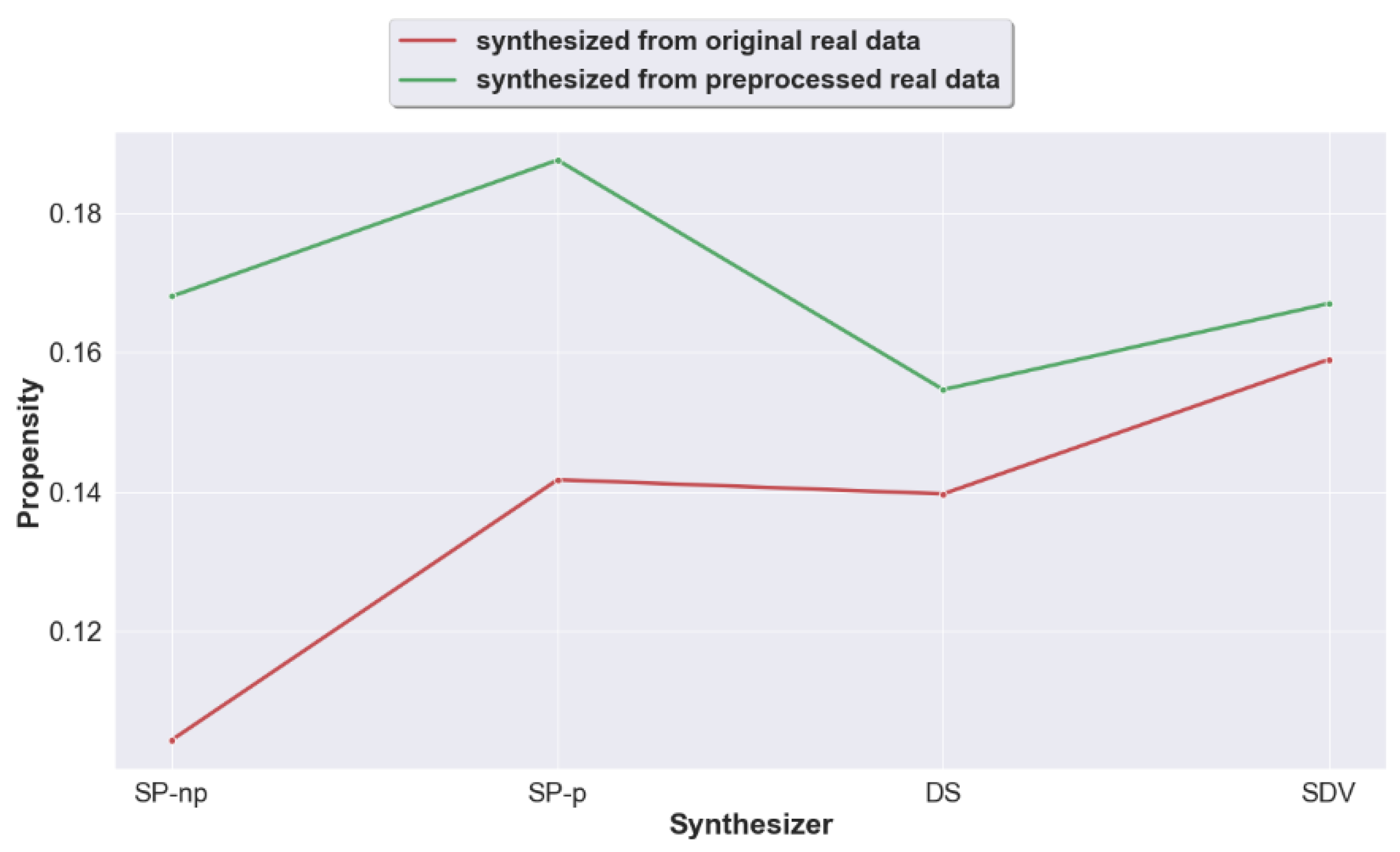
To answer this question, we compare the propensity score of data synthesized from raw real data (Path 1) using the four generators, versus the propensity score of data synthesized from preprocessed real data (Path 2). The results are shown in Figure 3 and Figure 4.
As evident from Figure 3, Propensity scores display a preference to data synthesized from raw real datasets across all synthesizers and particularly for the SP synthesizers. When we take the average propensity score across all datasets (Figure 4), this conclusion becomes more evident. Thus, overall, propensity scores display better results when data is synthesized from raw real datasets.
This result supports what has been followed in the literature, i.e., synthesizing from original raw data, and it also supports the desires of data scientists to have a dataset that looks like the original, and offers them the power to pre-process as they wish.
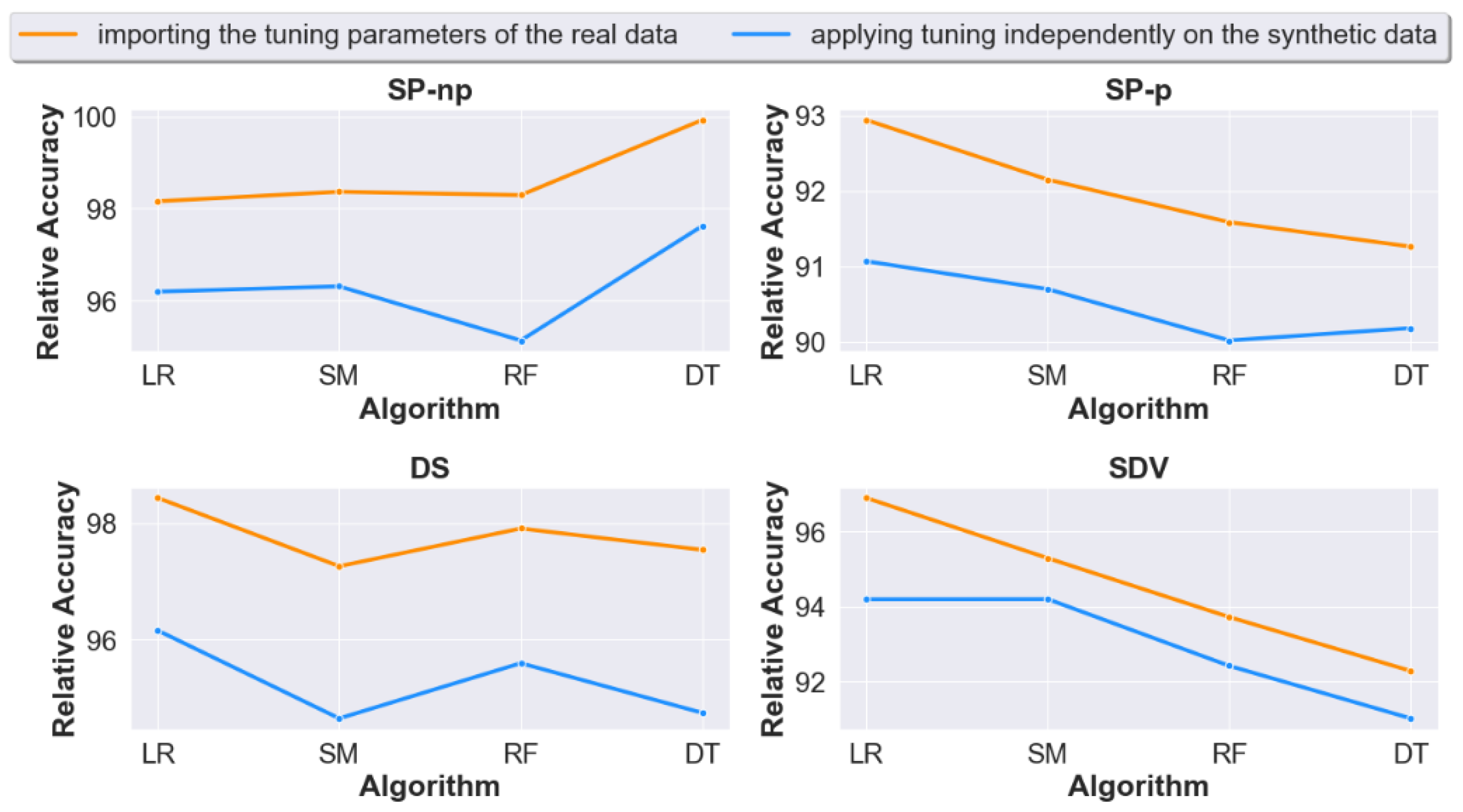
4.2. Question 2: When Calculating Prediction Accuracy, Does Importing the Real Data Tuning Settings to the Generated Synthetic Data Lead to Improved Accuracy Results?
The aim of this question is to guide data holders on whether to include additional information when sharing synthetic data. Such information can be shared at a later stage, once scientists have a decision regarding the methods and algorithms to run on the data.
To answer this question, we study the relative accuracy of the synthetic datasets in Case 1 versus Case 2 using the four aforementioned machine learning algorithms.
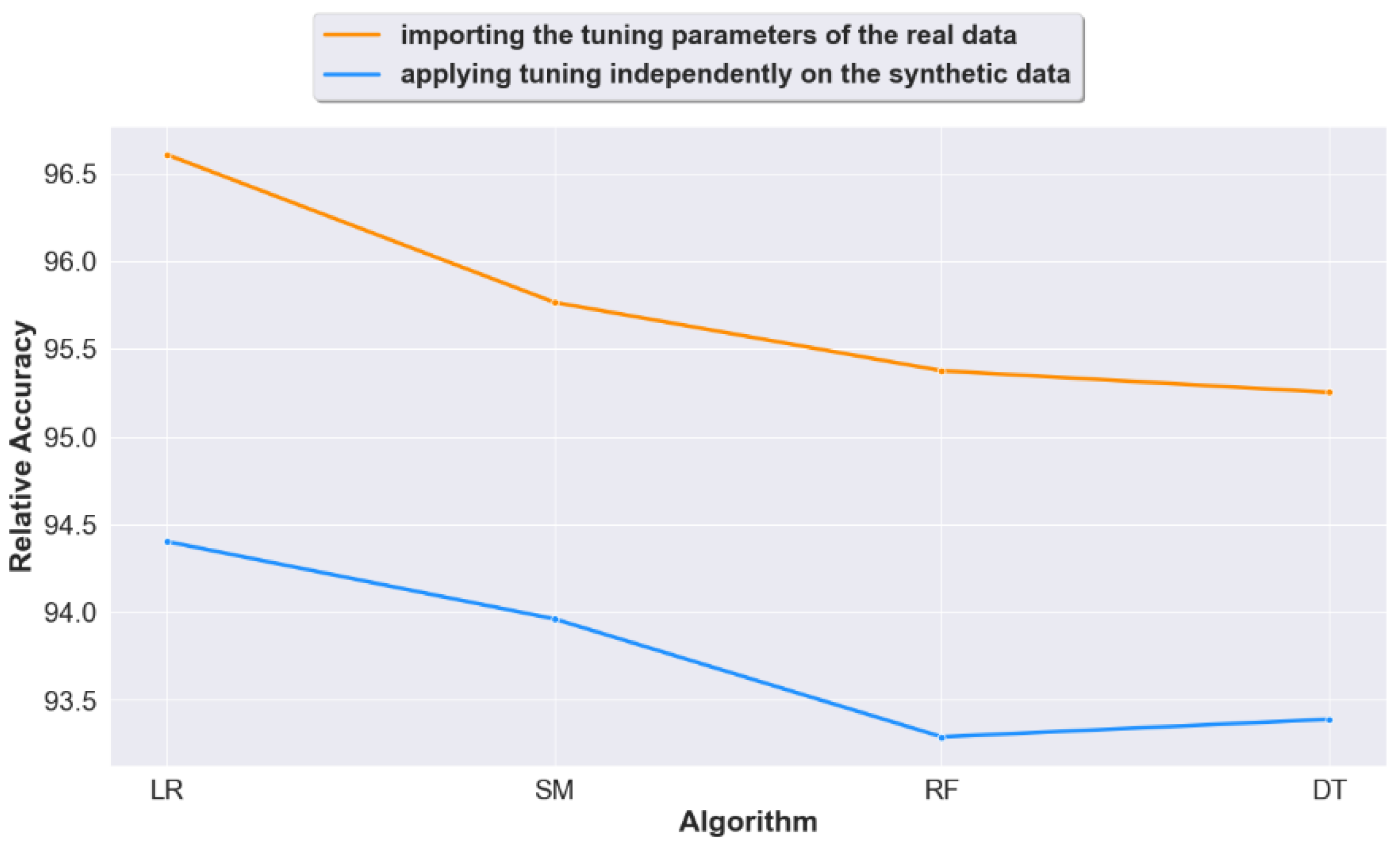
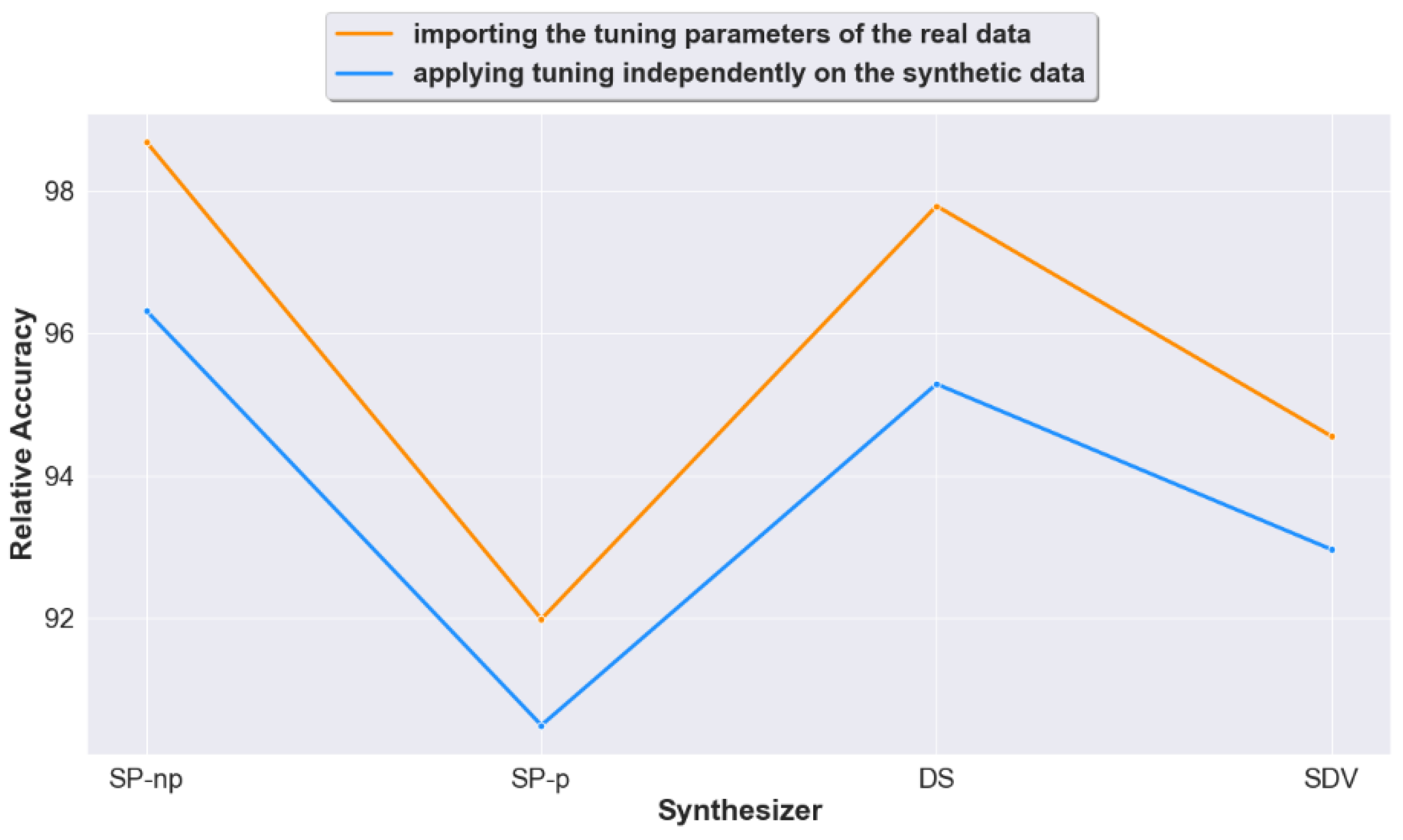
The results are shown in Figure 5, Figure 6 and Figure 7. Relative accuracy represents the synthetic data accuracy relative to the real data accuracy (100× synthetic accuracy/real accuracy).
Figure 5 shows that case 1 offers better accuracy across all ML algorithms and for all synthesizers.
Figure 6 shows the results from a different perspective. It displays the accuracy average across the four synthesizers, it shows an overall increase in accuracy when real data tuning is imported.
When taken per synthesizer (Figure 7), and as expected, Case 1 shows an overall better accuracy across all synthesizers.
4.3. Question 3: Should We Apply Tuning on the Synthetic Datasets Generated from Raw Unprocessed Data? Or Would Non-Tuning Lead to a Better Accuracy?
In general, parameter tuning and feature selection is essential to achieve high quality models. It is often the case that applying “out-of-the-box” machine learning algorithms to the data leads to inferior results [46].
However, with synthetic data, parameters are optimized using the synthetic data itself and final utility is tested on the real data. Therefore, if the synthetic data is generated from an inaccurate or biased model, the optimized parameters could further this bias, leading to low utility (on real data). As tuning is a highly time-consuming activity, it is essential to guide scientists working with synthetic data on the value of tuning their datasets.
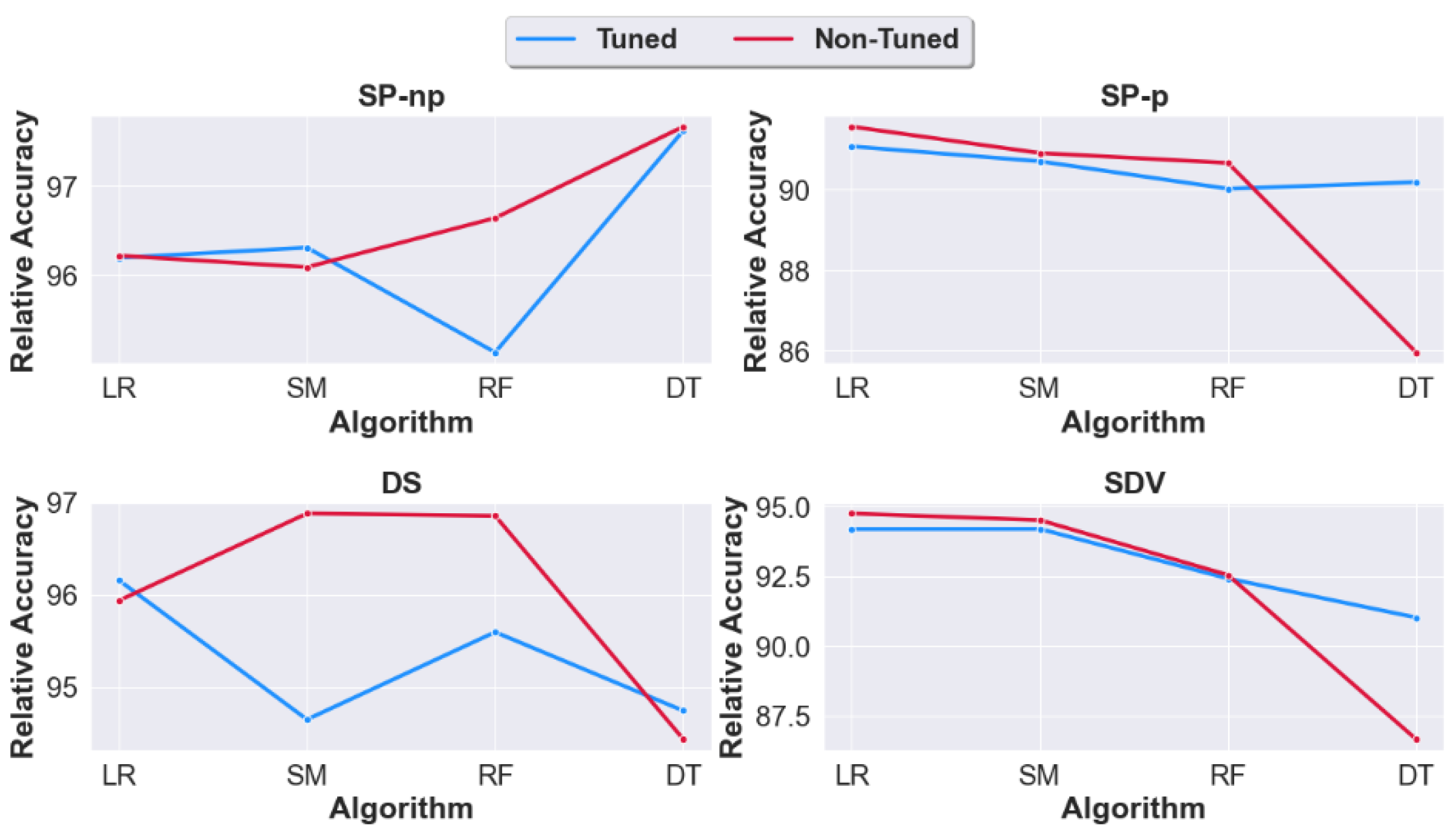
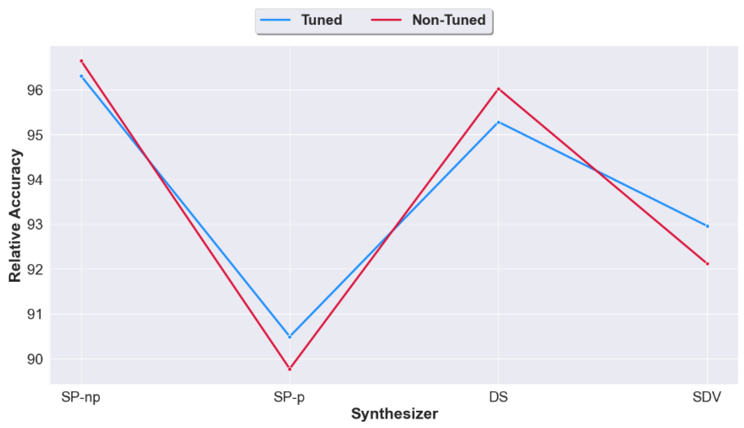
To best answer this question, we study the relative accuracy of the machine learning models with and without tuning (in other words we compare Case 2 and Case 3). For the non-tuned dataset, training is performed using the default parameters. The results of the experiments are shown in Figure 8, Figure 9 and Figure 10.
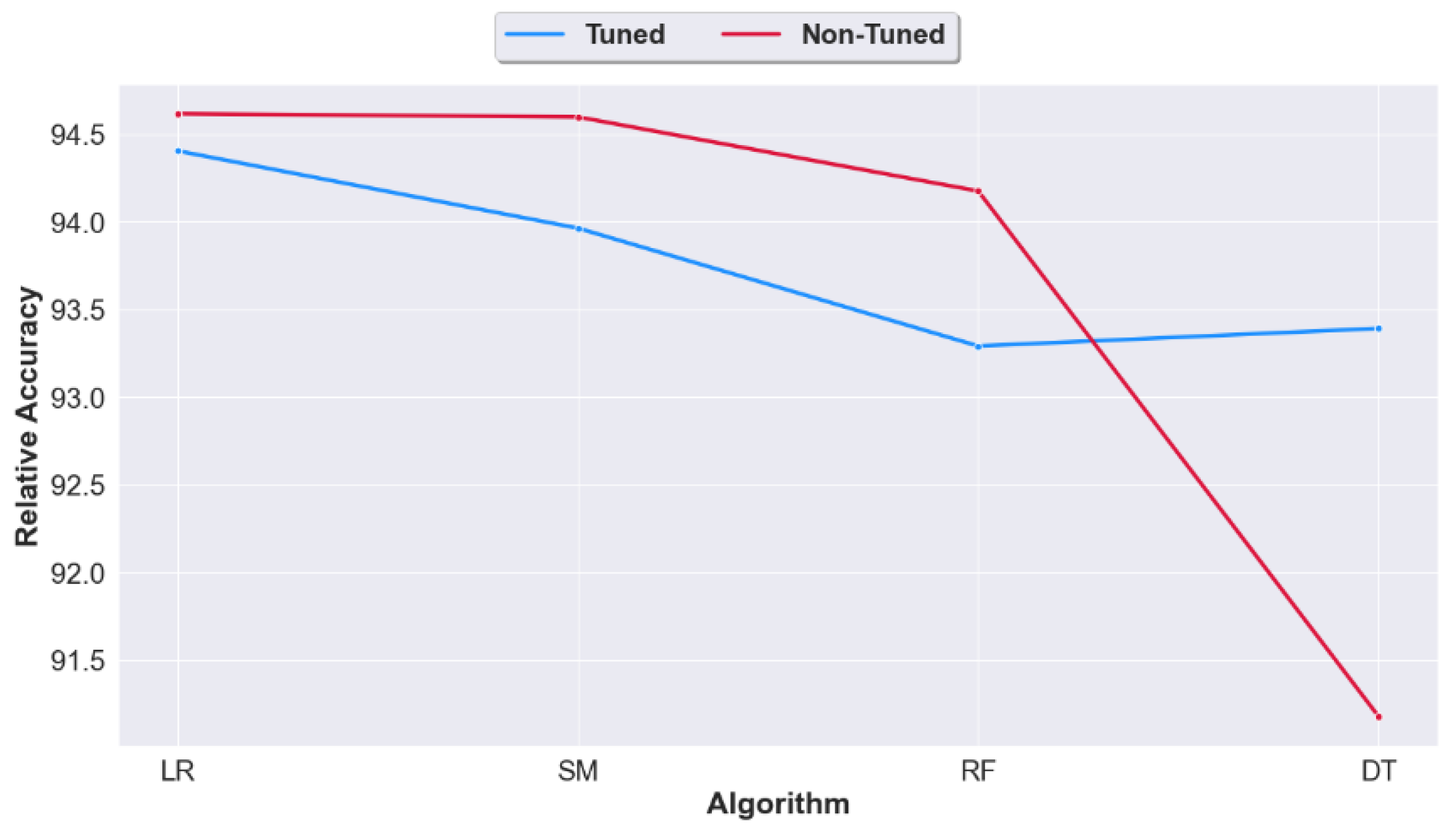
Figure 8 indicates similar accuracy for both with an overall preference to no tuning across all classification algorithms except DT. This conclusion is more evident in Figure 9 when the average is taken across all synthesizers.
Figure 10 displays the average accuracy across all classification algorithms, and shows slight differences between the two models across all datasets. Thus, we can deduce that overall, there is no evidence for synthetic datasets tuning (except when using DT).
4.4. Question 4: Is Propensity Score a Good Indicator for Prediction Accuracy?
Although various synthetic data generators have been developed in literature, empirical evidence of their utility has not been fully explored. Various measures for synthetic data utility exist in the literature, some are considered global measures (focusing on the features of the entire dataset) [41], others are analysis specific measures (to assess the utility in replicating a specific analysis done on real data) [30], and some are process related measures (these are measure related to the data generation technique used itself such as bias and stability [33]). The existence of one measure that accurately predicts synthetic data utility is beneficial on multiple fronts. It would allow data holders and scientists to concentrate on this one measure when assessing synthetic data utility. It would also enable data holders to include such measure in the data generation process as an optimization parameter.
Propensity score, has been cited as the best measure for the global utility of synthetic data, as such, we examine empirically whether propensity can be a strong predictor of classification accuracy across the different synthesizers.
Table 2 reports on the propensity scores as well as the difference in accuracy between real and synthetic datasets across all four machine learning algorithms. Propensity is taken for Path 2 (data synthesized from raw original data), and accuracy is taken for Case 3 (default settings) as tested on the real data.
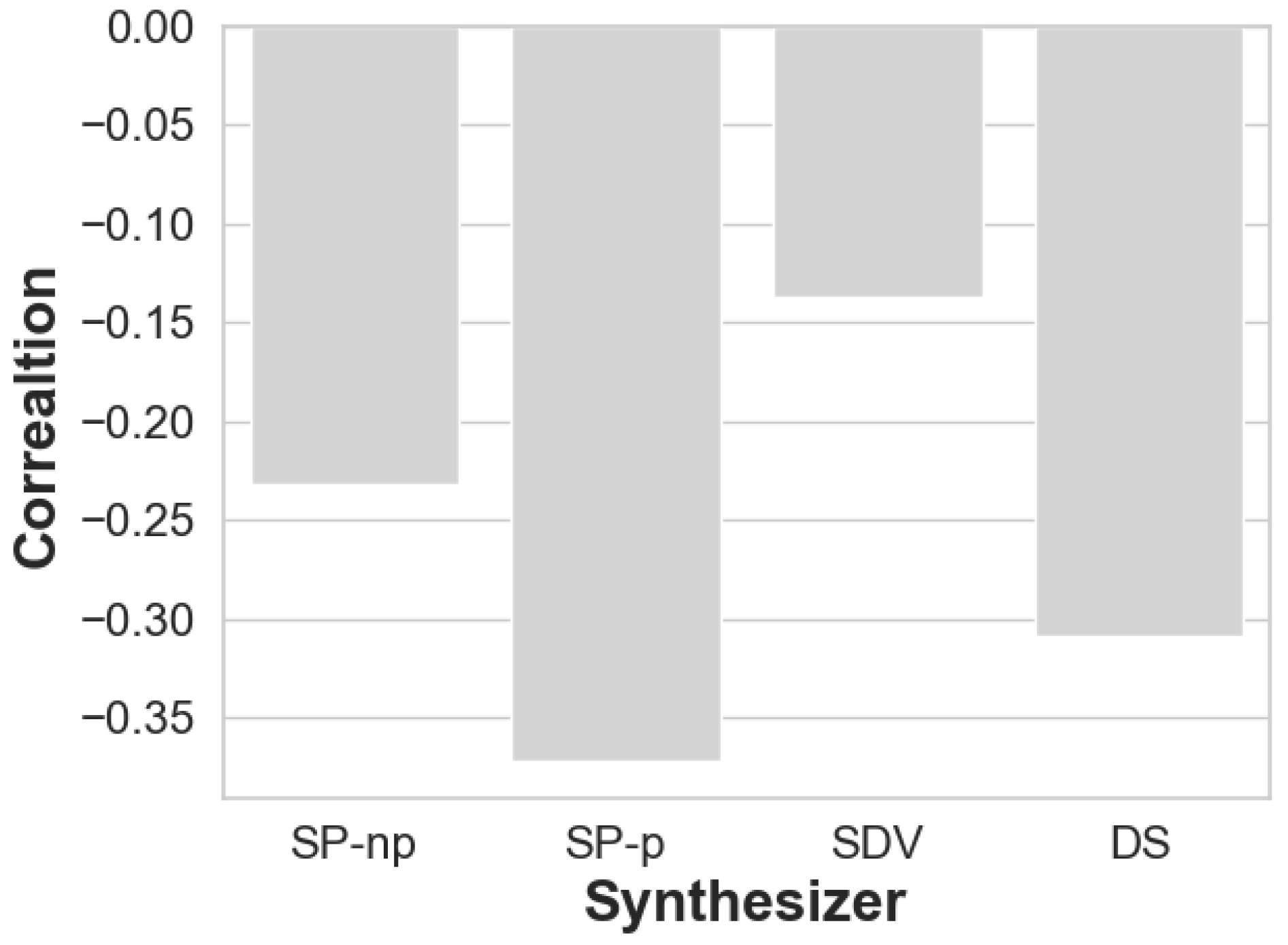
The correlation between these values (propensity and accuracy difference) is depicted in Figure 11 As expected, the correlation is always negative. As for strength, it is of moderate degree for SP-p, of low degree for DS and SP-np and weak for SDV [47].
Table 3, reports on the overall propensity scores, accuracy difference and relative accuracy per synthesizer. The values represent the average across the 15 datasets and the four machine learning algorithms. The table is ordered by relative accuracy and AD. The overall results suggest an agreement between propensity and accuracy for all synthesizers except SDV (SDV shows better accuracy than SP-p, although it has slightly lower propensity).
When taken together, the results suggest that propensity score may be a reliable forecaster for prediction accuracy for SP-p and DS, and less so for SP-np, but may not be a good accuracy predictor for synthetic data generated from SDV.
5. Conclusions
Synthetic data is still in the experimental stage and is often used to carry out preliminary research such as exploratory analyses or for the public release of data (such as census data, data used for education purposes, and data used in competitions). It is often the case that the final research analysis is obtained from the original dataset [48].
To understand whether synthetic data can be used for more than the exploratory data analysis tasks, an exploration into the utility of synthetic data needs to be done. That includes investigations into the efficiency of data synthesis methods, comparisons between synthetic data generation methods and other privacy enhancing technologies, as well as investigations into the best data generation settings/paths. While the first and second points are the subject of recent investigations (with the second being less explored but starting to get more attention), the third point has not yet been explored in prior research. As such, in this article, we investigate different synthetic data generation settings with a goal to guide data holders into the best synthetic data generation and usage path.
Our results show that there is no benefit from pre-processing real data prior to synthesizing it (Q1). Switching to Machine learning models, our results show that tuning the ML models when using synthetic datasets (versus default parameters and features) does not enhances the performance of the generated models (Q3). However, importing the real data tuning-settings onto the synthetic data models is beneficial and presented an improvement in accuracy across all generators. This signifies a benefit in sharing the tuning setting of the real data along with the synthetic data, once/if the user is aware of the type of analysis to be performed on the data (Q2). Lastly, our results suggest that propensity scores are good forecasters for prediction accuracy when the synthetic data is generated using SP-p and DS synthesizers, which could be helpful for data holders in benchmarking their synthetic datasets generated via SP-p and DS (Q4).
To summarize the above, these preliminary experiments suggest that there is no need to tune synthetic data when using supervised machine learning models, that it may be beneficial to share some “privacy-safe” pre-classification results along with the synthetic data, and that propensity score is a sufficient predictor of accuracy when using the SP-p and DS generators.
It is important to note that our results are limited by our testing strategies. Some of these questions are more complex in real life than what is being tested. For example, there are more approaches for preprocessing available to analysts than what was assumed in the experiments. Our goal from this paper was to raise these pertinent questions as much as to try to tackle them from certain dimensions. More experiments should be done to assert and strengthen the obtained results with a purpose to inform on the best synthetic data pipeline.
Author Contributions
Conceptualization, F.K.D.; methodology, F.K.D.; software, F.K.D. and M.I.; validation, F.K.D. and M.I.; formal analysis, F.K.D.; investigation, F.K.D.; resources, F.K.D. and M.I.; data curation, F.K.D. and M.I.; writing—original draft preparation, F.K.D.; writing—review and editing, F.K.D.; visualization, F.K.D. and M.I.; supervision, F.K.D.; project administration, F.K.D.; funding acquisition, F.K.D. All authors have read and agreed to the published version of the manuscript.
Funding
This research was funded by UAE University research grant UPAR # 31T121.
Institutional Review Board Statement
Not applicable.
Informed Consent Statement
Not applicable.
Data Availability Statement
Publicly available datasets were analyzed in this study. This data can be found here: University of California Irvine repository (https://archive.ics.uci.edu/, accessed on 1 February 2021), OpenML platform (https://www.openml.org/, accessed on 1 February 2021), and Kaggle community platform (https://www.kaggle.com/, accessed on 1 February 2021).
Conflicts of Interest
The authors declare no conflict of interest.
References
- Davenport, T.; Kalakota, R. The potential for artificial intelligence in healthcare. Future Healthc. J. 2019, 6, 94–98. [Google Scholar] [CrossRef] [Green Version]
- Lysaght, T.; Lim, H.Y.; Xafis, V.; Ngiam, K.Y. AI-Assisted Decision-making in Healthcare. Asian Bioeth. Rev. 2019, 11, 299–314. [Google Scholar] [CrossRef] [Green Version]
- McGlynn, E.A.; Lieu, T.A.; Durham, M.L.; Bauck, A.; Laws, R.; Go, A.S.; Chen, J.; Feigelson, H.S.; Corley, D.A.; Young, D.R.; et al. Developing a data infrastructure for a learning health system: The PORTAL network. J. Am. Med. Inform. Assoc. JAMIA 2014, 21, 596–601. [Google Scholar] [CrossRef] [Green Version]
- Use of Artificial Intelligence in Infectious Diseases. Available online: https://0-www-ncbi-nlm-nih-gov.brum.beds.ac.uk/pmc/articles/PMC7153335/ (accessed on 18 February 2021).
- Dankar, F.K.; el Emam, K.; Neisa, A.; Roffey, T. Estimating the re-identification risk of clinical data sets. BMC Med. Inform. Decis. Mak. 2012, 12, 66. [Google Scholar] [CrossRef] [Green Version]
- GDPR. General Data Protection Regulation (GDPR). 2018. Available online: https://gdpr-info.eu/ (accessed on 9 December 2018).
- U.S. Department of Health & Human Services. Available online: http://www.hhs.gov/ (accessed on 22 September 2015).
- Dankar, F.K.; Gergely, M.; Dankar, S.K. Informed Consent in Biomedical Research. Comput. Struct. Biotechnol. J. 2019, 17, 463–474. [Google Scholar] [CrossRef] [PubMed]
- Artificial Intelligence In Health Care: Benefits and Challenges of Machine Learning in Drug Development (STAA)-Policy Briefs & Reports-EPTA Network. Available online: https://eptanetwork.org/database/policy-briefs-reports/1898-artificial-intelligence-in-health-care-benefits-and-challenges-of-machine-learning-in-drug-development-staa (accessed on 1 September 2020).
- Howe, B.; Stoyanovich, J.; Ping, H.; Herman, B.; Gee, M. Synthetic Data for Social Good. arXiv 2017, arXiv:171008874. [Google Scholar]
- Mostert, M.; Bredenoord, A.L.; Biesaart, M.C.; van Delden, J.J. Big Data in medical research and EU data protection law: Challenges to the consent or anonymise approach. Eur. J. Hum. Genet. 2016, 24, 956. [Google Scholar] [CrossRef]
- Dankar, F.K.; Ptitsyn, A.; Dankar, S.K. The development of large-scale de-identified biomedical databases in the age of genomics—principles and challenges. Hum. Genom. 2018, 12, 19. [Google Scholar] [CrossRef]
- Dankar, F.K.; Badji, R. A risk-based framework for biomedical data sharing. J. Biomed. Inform. 2017, 66, 231–240. [Google Scholar] [CrossRef] [PubMed]
- Ervine, C. Directive 2004/39/Ec of the European Parliament and of the Council of 21 April 2004. In Core Statutes on Company Law; Macmillan Education: London, UK, 2015; pp. 757–759. [Google Scholar]
- Naveed, M.; Ayday, E.; Clayton, E.W.; Fellay, J.; Gunter, C.A.; Hubaux, J.P.; Malin, B.A.; Wang, X. Privacy in the genomic era. ACM Comput. Surv. CSUR 2015, 48, 6. [Google Scholar] [CrossRef] [PubMed]
- Dankar, F.K.; Gergely, M.; Malin, B.; Badji, R.; Dankar, S.K.; Shuaib, K. Dynamic-informed consent: A potential solution for ethical dilemmas in population sequencing initiatives. Comput. Struct. Biotechnol. J. 2020, 18, 913–921. [Google Scholar] [CrossRef]
- Taub, J.; Elliot, M.; Pampaka, M.; Smith, D. Differential Correct Attribution Probability for Synthetic Data: An Exploration. In Privacy in Statistical Databases; Springer: Cham, Spain, 2018; pp. 122–137. [Google Scholar] [CrossRef]
- Data Synthesis Based on Generative Adversarial Networks|Proceedings of the VLDB Endowment. Available online: https://0-dl-acm-org.brum.beds.ac.uk/doi/10.14778/3231751.3231757 (accessed on 1 September 2020).
- Rubin, D.B. Statistical disclosure limitation. J. Off. Stat. 1993, 9, 461–468. [Google Scholar]
- Ruiz, N.; Muralidhar, K.; Domingo-Ferrer, J. On the Privacy Guarantees of Synthetic Data: A Reassessment from the Maximum-Knowledge Attacker Perspective. In Privacy in Statistical Databases; Springer: Cham, Spain, 2018; pp. 59–74. [Google Scholar] [CrossRef]
- Hu, J. Bayesian Estimation of Attribute and Identification Disclosure Risks in Synthetic Data. arXiv 2018, arXiv:180402784. [Google Scholar]
- Polonetsky, J.; Elizabeth, R. 10 Privacy Risks and 10 Privacy Technologies to Watch in the Next Decade. Presented at the Future of Privacy Forum. 2020. Available online: https://fpf.org/wp-content/uploads/2020/01/FPF_Privacy2020_WhitePaper.pdf (accessed on 26 February 2021).
- Patki, N.; Wedge, R.; Veeramachaneni, K. The Synthetic Data Vault. In Proceedings of the 2016 IEEE International Conference on Data Science and Advanced Analytics (DSAA), Montreal, QC, Canada, 17–19 October 2016; pp. 399–410. [Google Scholar] [CrossRef]
- Ping, H.; Stoyanovich, J.; Howe, B. Datasynthesizer: Privacy-preserving synthetic datasets. In Proceedings of the 29th International Conference on Scientific and Statistical Database Management, Chicago, IL, USA, 27–29 June 2017; pp. 1–5. [Google Scholar]
- Raab, G.M.; Nowok, B.; Dibben, C. Guidelines for Producing Useful Synthetic Data. arXiv 2017, arXiv:171204078. [Google Scholar]
- Yoon, J.; Drumright, L.N.; van der Schaar, M. Anonymization through Data Synthesis using Generative Adversarial Networks (ADS-GAN). IEEE J. Biomed. Health Inform. 2020, 24, 2378–2388. [Google Scholar] [CrossRef]
- Rankin, D.; Black, M.; Bond, R.; Wallace, J.; Mulvenna, M.; Epelde, G. Reliability of Supervised Machine Learning Using Synthetic Data in Health Care: Model to Preserve Privacy for Data Sharing. JMIR Med. Inform. 2020, 8, e18910. [Google Scholar] [CrossRef] [PubMed]
- Hittmeir, M.; Ekelhart, A.; Mayer, R. Utility and Privacy Assessments of Synthetic Data for Regression Tasks. In Proceedings of the 2019 IEEE International Conference on Big Data (Big Data), Los Angeles, CA, USA, 9–12 December 2019; pp. 5763–5772. [Google Scholar]
- Nowok, B. Utility of Synthetic Microdata Generated Using Tree-Based Methods. UNECE Stat. Data Confidentiality Work Sess. 2015. Available online: https://unece.org/fileadmin/DAM/stats/documents/ece/ces/ge.46/20150/Paper_33_Session_2_-_Univ._Edinburgh__Nowok_.pdf (accessed on 26 February 2021).
- Hittmeir, M.; Ekelhart, A.; Mayer, R. On the utility of synthetic data: An empirical evaluation on machine learning tasks. In Proceedings of the 14th International Conference on Availability, Reliability and Security, Canterbury, UK, 26–29 August 2019; pp. 1–6. [Google Scholar]
- Dandekar, A.; Zen, R.A.; Bressan, S. Comparative Evaluation of Synthetic Data Generation Methods. Available online: https://www.di.ens.fr/~adandekar/files/papers/data_gen.pdf (accessed on 26 February 2021).
- Drechsler, J. Synthetic Datasets for Statistical Disclosure Control: Theory and Implementation; Springer: New York, NY, USA, 2011. [Google Scholar]
- Benaim, A.R.; Almog, R.; Gorelik, Y.; Hochberg, I.; Nassar, L.; Mashiach, T.; Khamaisi, M.; Lurie, Y.; Azzam, Z.S.; Khoury, J.; et al. Analyzing Medical Research Results Based on Synthetic Data and Their Relation to Real Data Results: Systematic Comparison From Five Observational Studies. JMIR Med. Inform. 2020, 8. [Google Scholar] [CrossRef]
- Heyburn, R.; Bond, R.; Black, M.; Mulvenna, M.; Wallace, J.; Rankin, D.; Cleland, B. Machine learning using synthetic and real data: Similarity of evaluation metrics for different healthcare datasets and for different algorithms. Data Sci. Knowl. Eng. Sens. Decis. Support 2018, 1281–1291. [Google Scholar]
- Nowok, B.; Raab, G.M.; Dibben, C. synthpop: Bespoke creation of synthetic data in R. J. Stat. Softw. 2016, 74, 1–26. [Google Scholar] [CrossRef] [Green Version]
- PrivBayes: Private Data Release via Bayesian Networks: ACM Transactions on Database Systems: Vol 42, No 4. Available online: https://0-dl-acm-org.brum.beds.ac.uk/doi/10.1145/3134428 (accessed on 24 December 2020).
- Trivedi, P.K.; Zimmer, D.M. Copula Modeling: An Introduction for Practitioners; Now Publishers Inc.: Hanover, MA, USA, 2007. [Google Scholar]
- General and Specific Utility Measures for Synthetic Data-Snoke-2018-Journal of the Royal Statistical Society: Series A (Statistics in Society)-Wiley Online Library. Available online: https://0-rss-onlinelibrary-wiley-com.brum.beds.ac.uk/doi/full/10.1111/rssa.12358 (accessed on 19 November 2020).
- Practical Synthetic Data Generation [Book]. Available online: https://www.oreilly.com/library/view/practical-synthetic-data/9781492072737/ (accessed on 6 September 2020).
- Snoke, J.; Raab, G.; Nowok, B.; Dibben, C.; Slavkovic, A. General and specific utility measures for synthetic data. arXiv 2017, arXiv:160406651. [Google Scholar] [CrossRef] [Green Version]
- Woo, M.-J.; Reiter, J.P.; Oganian, A.; Karr, A.F. Global Measures of Data Utility for Microdata Masked for Disclosure Limitation. J. Priv. Confid. 2009, 1. [Google Scholar] [CrossRef] [Green Version]
- Westreich, D.; Lessler, J.; Funk, M.J. Propensity score estimation: Neural networks, support vector machines, decision trees (CART), and meta-classifiers as alternatives to logistic regression. J. Clin. Epidemiol. 2010, 63, 826–833. [Google Scholar] [CrossRef] [Green Version]
- Rosenbaum, P.R.; Rubin, D.B. Reducing Bias in Observational Studies Using Subclassification on the Propensity Score. J. Am. Stat. Assoc. 1984, 79, 516–524. [Google Scholar] [CrossRef]
- El Emam, K. Seven Ways to Evaluate the Utility of Synthetic Data. IEEE Secur. Priv. 2020, 18, 56–59. [Google Scholar] [CrossRef]
- Reiter, J.P. Using CART to generate partially synthetic public use microdata. J. Off. Stat. 2005, 21, 441. [Google Scholar]
- Raschka, S. Model evaluation, model selection, and algorithm selection in machine learning. arXiv 2018, arXiv:181112808. [Google Scholar]
- Konen, W.; Koch, P.; Flasch, O.; Bartz-Beielstein, T.; Friese, M.; Naujoks, B. Tuned data mining: A benchmark study on different tuners. In Proceedings of the 13th Annual Conference on Genetic and Evolutionary Computation, New York, NY, USA, 9–13 July 2011; pp. 1995–2002. [Google Scholar] [CrossRef]
- Taylor, R. Interpretation of the Correlation Coefficient: A Basic Review. J. Diagn. Med. Sonogr. 1990, 6, 35–39. [Google Scholar] [CrossRef]
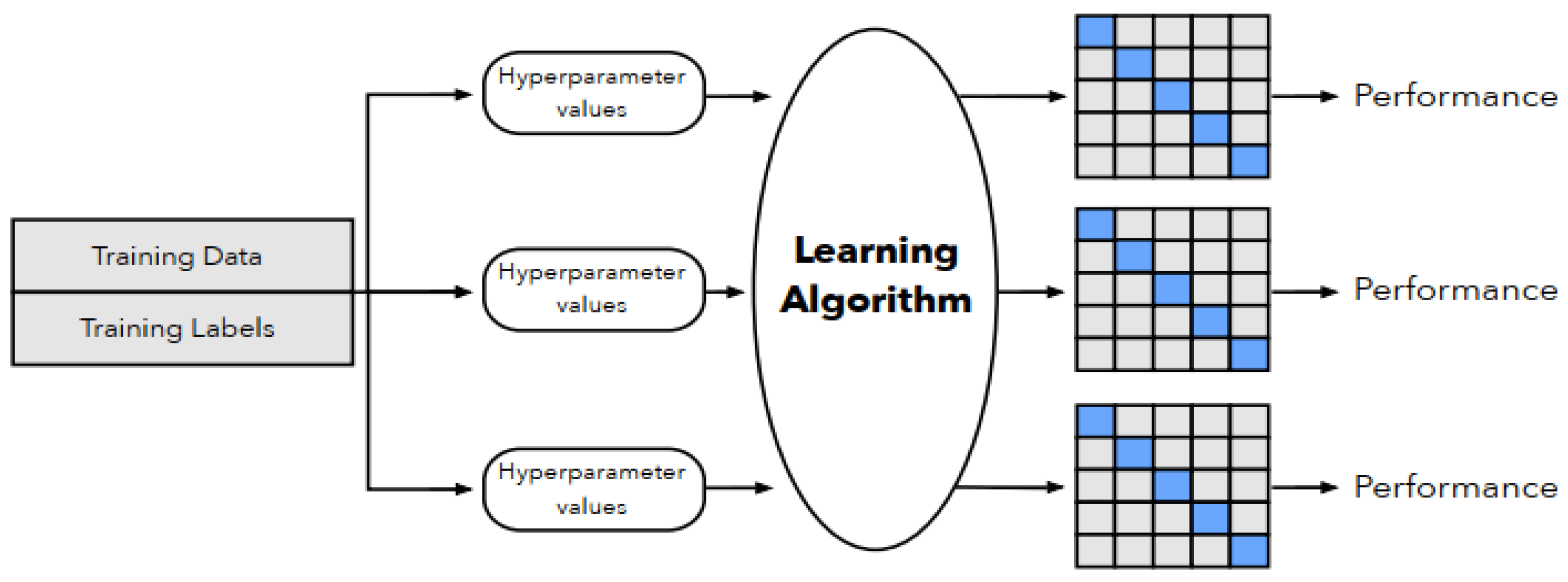
Figure 1.
A representation of 5 folds cross validation method. The figure shows the first step of the method, which consists of forming sets of different hyperparameter values. The Figure is taken from [43].
Figure 1.
A representation of 5 folds cross validation method. The figure shows the first step of the method, which consists of forming sets of different hyperparameter values. The Figure is taken from [43].

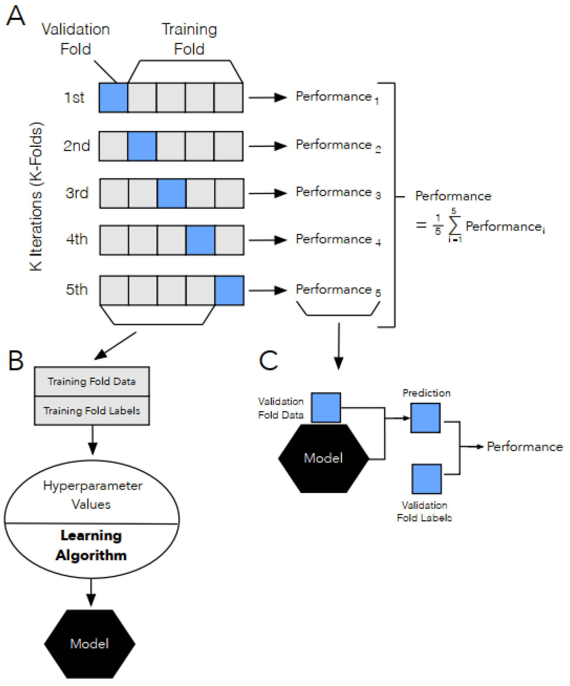
Figure 2.
Details of 5 folds cross validation method for a given set of hyperparameter values. Where the steps consist of: Dividing the synthetic dataset SD randomly into 5 equal subsets or folds (A). Then, for each hyperparameter values-set, the model is trained 5 times using a different testing (or validation) fold every time (4 folds are used as training and one is used for validation) (A,B). The average of the performance metrics is then reported (A). The hyperparameter set that gives the best average performance is chosen to produce the final model (C). The final model is then tested on the real testing data. The Figure is taken from [43].

Figure 3.
Propensity scores per dataset across all classification algorithms. The x-axis represents the different datasets ordered according to their attributes number .
Figure 3.
Propensity scores per dataset across all classification algorithms. The x-axis represents the different datasets ordered according to their attributes number .

Figure 4.
Propensity scores per synthesizer (across datasets).

Figure 5.
Relative accuracy for each synthesizer across all datasets for cases 1 and 2. The x-axis represents the ML model.
Figure 5.
Relative accuracy for each synthesizer across all datasets for cases 1 and 2. The x-axis represents the ML model.

Figure 6.
Relative accuracy across all synthesizers and all datasets for each ML model.

Figure 7.
Relative accuracy across all ML models and all datasets for each synthesizer.

Figure 8.
Relative accuracy of the ML models for each synthesizer across all datasets. Tuned and non-tuned case.
Figure 8.
Relative accuracy of the ML models for each synthesizer across all datasets. Tuned and non-tuned case.

Figure 9.
Relative accuracy of the ML models across all synthesizer and datasets. Tuned and non-tuned case.
Figure 9.
Relative accuracy of the ML models across all synthesizer and datasets. Tuned and non-tuned case.

Figure 10.
Relative accuracy of the synthesizers across all ML models and datasets. Tuned and non-tuned case.
Figure 10.
Relative accuracy of the synthesizers across all ML models and datasets. Tuned and non-tuned case.

Figure 11.
Correlation coefficients per synthesizer.


Table 1.
Datasets description.
| Dataset Name | Short Name | Number of Observations | Number of Attributes (Predictors) | Categorical Predictors | Number of Labels | Total Synthetic Datasets Generated | Origin |
|---|---|---|---|---|---|---|---|
| BankNote | 1372 | 4 | 0 | 2 | 160 | UCI | |
| Titanic | 891 | 7 | 7 | 2 | 160 | Kaggle | |
| Ecoli | 336 | 7 | 0 | 8 | 160 | UCI | |
| Diabetes | 768 | 9 | 2 | 2 | 160 | UCI | |
| Cleveland heart | 297 | 13 | 8 | 2 | 160 | UCI | |
| Adult | 48,843 | 14 | 8 | 2 | 144 1 | UCI | |
| Breast cancer | 570 | 30 | 0 | 2 | 160 | UCI | |
| Dermatology | 366 | 34 | 33 | 6 | 160 | UCI | |
| SPECTF Heart | 267 | 44 | 0 | 2 | 160 | UCI | |
| Z-Alizadeh Sani | 303 | 55 | 34 | 2 | 160 | UCI | |
| Colposcopies | 287 | 68 | 6 | 2 | 160 | UCI | |
| ANALCATDATA | 841 | 71 | 3 | 2 | 160 | OpenML | |
| Mice Protein | 1080 | 80 | 3 | 8 | 160 | UCI | |
| Diabetic Mellitus | 281 | 97 | 92 | 2 | 135 2 | OpenML | |
| Tecator | 240 | 124 | 0 | 2 | 160 3 | OpenML |
1 24 synthetic datasets were generated for DS due to time inefficiency. 2 15 synthetic datasets were generated for SDV due to time inefficiency; 3 For DS, the number of parents’ nodes allowed was changed from default to 2 due to time inefficiency.
Table 2.
Propensity (Prop) and accuracy difference (AD) for each [dataset, synthesizer] pairs. AD is calculated as [average real accuracy- average synthetic accuracy].
Table 2.
Propensity (Prop) and accuracy difference (AD) for each [dataset, synthesizer] pairs. AD is calculated as [average real accuracy- average synthetic accuracy].
| SP-np | SP-p | SDV | DS | |||||
|---|---|---|---|---|---|---|---|---|
| AD | Prop | AD | Prop | AD | Prop | AD | Prop | |
| 1.031553 | 0.074972 | 3.4375 | 0.155349 | 2.038835 | 0.155198 | 0.039442 | 0.099199 | |
| 0.037313 | 0.074571 | 2.103545 | 0.119064 | 4.650187 | 0.132735 | −0.46642 | 0.128916 | |
| 4.009901 | 0.075293 | 3.589109 | 0.108319 | 9.034653 | 0.157922 | 2.487624 | 0.165095 | |
| 2.288961 | 0.08493 | 4.821429 | 0.09705 | 6.504329 | 0.133996 | 2.505411 | 0.098722 | |
| 2.388889 | 0.086021 | 3.583333 | 0.095108 | 2.472222 | 0.152168 | 1.347222 | 0.154571 | |
| −0.41583 | 0.004673 | 4.805833 | 0.031423 | 6.4375 | 0.11616 | 2.659167 | 0.025647 | |
| 2.295322 | 0.128166 | 3.092105 | 0.191422 | 3.79386 | 0.155758 | 3.347953 | 0.159778 | |
| 5.363636 | 0.083088 | 43.65909 | 0.154837 | 8.684211 | 0.129181 | 1.113636 | 0.066643 | |
| 1.095679 | 0.132029 | 1.496914 | 0.144961 | 2.037037 | 0.142773 | 2.052469 | 0.118727 | |
| 10.26099 | 0.124009 | 11.78571 | 0.128848 | 10.6044 | 0.161104 | 8.873626 | 0.151974 | |
| 7.241379 | 0.153457 | 12.52874 | 0.178307 | 8.390805 | 0.234168 | 5.402299 | 0.233867 | |
| −6.03261 | 0.138881 | −7.67787 | 0.146417 | −3.57812 | 0.193994 | 1.215415 | 0.145242 | |
| 5.9825 | 0.171316 | 15.485 | 0.195285 | 25.8875 | 0.194417 | 5.6475 | 0.248655 | |
| 0.735294 | 0.112665 | 14.66176 | 0.143493 | 11.07353 | 0.166697 | 2.566845 | 0.140432 | |
| 10.88542 | 0.121138 | 26.63194 | 0.235745 | 9.809028 | 0.158509 | 14.44444 | 0.157601 | |
Table 3.
The Propensity, relative accuracy and accuracy difference scores for each synthesizer. The table is ordered by accuracy and the number in bracket next to propensity scores indicate their order (note that lower propensity indicates better utility).
Table 3.
The Propensity, relative accuracy and accuracy difference scores for each synthesizer. The table is ordered by accuracy and the number in bracket next to propensity scores indicate their order (note that lower propensity indicates better utility).
| Case | Synthesizer | Rel Accuracy | AD | Prop |
|---|---|---|---|---|
| Synthesized from original real data Accuracy for Case 3 | SP-np | 96.653917 | 3.1445598 | 0.104347 (1) |
| DS | 96.025506 | 3.5491086 | 0.139671 (2) | |
| SDV | 92.117844 | 7.1893318 | 0.158985 (4) | |
| SP-p | 89.770557 | 9.60027587 | 0.141708 (3) |
Publisher’s Note: MDPI stays neutral with regard to jurisdictional claims in published maps and institutional affiliations. |
© 2021 by the authors. Licensee MDPI, Basel, Switzerland. This article is an open access article distributed under the terms and conditions of the Creative Commons Attribution (CC BY) license (http://creativecommons.org/licenses/by/4.0/).
Share and Cite
MDPI and ACS Style
Dankar, F.K.; Ibrahim, M. Fake It Till You Make It: Guidelines for Effective Synthetic Data Generation. Appl. Sci. 2021, 11, 2158. https://0-doi-org.brum.beds.ac.uk/10.3390/app11052158
AMA Style
Dankar FK, Ibrahim M. Fake It Till You Make It: Guidelines for Effective Synthetic Data Generation. Applied Sciences. 2021; 11(5):2158. https://0-doi-org.brum.beds.ac.uk/10.3390/app11052158
Chicago/Turabian StyleDankar, Fida K., and Mahmoud Ibrahim. 2021. "Fake It Till You Make It: Guidelines for Effective Synthetic Data Generation" Applied Sciences 11, no. 5: 2158. https://0-doi-org.brum.beds.ac.uk/10.3390/app11052158
Note that from the first issue of 2016, this journal uses article numbers instead of page numbers. See further details here.