Proposal of a Probabilistic Model on Rotating Bending Fatigue Property of a Bearing Steel in a Very High Cycle Regime

Abstract

In S-N diagrams for high strength steels, the duplex S-N curves for surface-initiated failure and interior inclusion-initiated failure were usually confirmed in the very high cycle regime. This trend is more distinct in the loading type of rotating bending, due to the stress distribution across the section. In the case of interior failure mode, the fish-eye is usually observed on the fracture surface and an inclusion is also observed at the center of the fish-eye. In the present work, the authors attempted to construct a probabilistic model on the statistical fatigue property in the interior failure mode, based on the distribution characteristics of the location and the size of the interior inclusion at the crack initiation site. Thus, the P-S-N characteristics of the bearing steel (SUJ2) in the very high cycle regime were successfully explained.

1. Introduction

From both viewpoints of economical design of mechanical structures and reduction of the environmental load, elongation of the design life for every product in the wide range of industries, is an important subject. In such a circumstance, for train axles and wheels, load bearing parts of automobiles, turbine rotors of the power plants and so on, the number of loading cycles reaches over 10⁹ cycles, during the service period of the respective mechanical components [1,2,3,4]. One of the typical aspects of fatigue property in the very high cycle regime for structural steels is the fact that the duplex S-N characteristics consisting of the respective S-N curves for the surface-initiated and the interior-initiated failures are observed, as reported by many researchers [3,5,6,7]. The term “S-N curve” refers to the relationship between the stress level [S] and the number of stress cycles to failure [N]. Expressions of S-N property and S-N characteristics are also used in this paper, based on a similar sense. In the case of interior-initiated failure, an inclusion is usually found at the core portion of the fish-eye formed on the fracture surface [3,5,8]. Thus, the interior inclusion at the crack initiation site plays a dominant role to govern the fatigue strength and fatigue life of the specimen.

It is well-known that the fatigue limit of the metallic material can be evaluated by combining the material hardness and the concept of $\sqrt{area}$ for the defect size proposed by Murakami et al. [9]. Another important factor to control the fatigue property is the location of the inclusion, since the stress distribution across the section has a steep slope in rotating bending [10]. Accordingly, the fatigue property of those metallic materials should be analyzed as a function of the size and the location of the interior inclusions, together with the hardness. However, both the size and the location of the inclusions inside the material have particular distributions, depending on the fabrication process of the actual metallic materials [11,12,13].

From this point of view, the authors attempted to construct a probabilistic model on the very high cycle fatigue property for the bearing steel of SUJ2 in rotating bending, by combining the distribution characteristics of the size and the location of the interior inclusion. In this model, a two-parameter Weibull distribution was accepted for the distribution pattern of the inclusion size, whereas the random distribution was accepted for the location of the inclusion. Since the scatter of the hardness is sufficiently small, the hardness of this steel was supposed to be constant for the sake of simplicity. Although some number of papers analyzing the statistical aspects of S-N property were published [14,15,16,17,18,19], the main target of those research is the statistical property within the usual life region, which is less than 10⁷ cycles. Considering this point, the main aim of the present study was set to the physical interpretation of the statistical aspects of the S-N characteristics of a bearing steel, in the very high cycle regime.

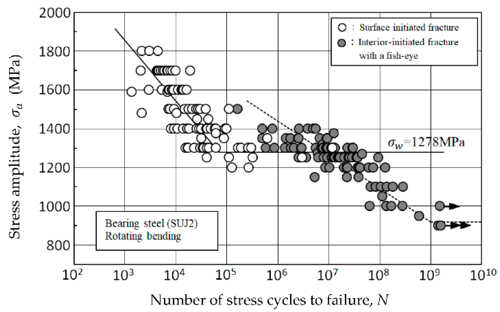
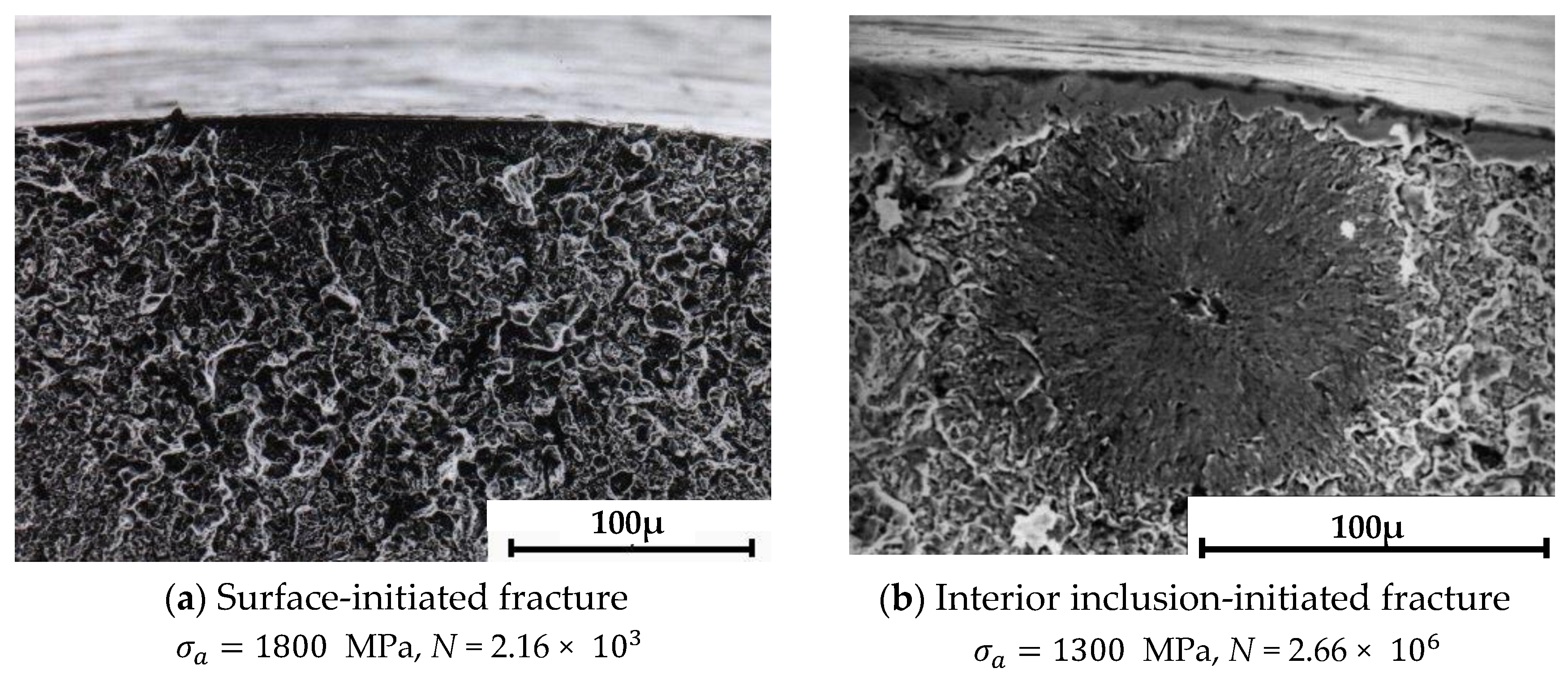
2. Experimental Fatigue Test Data Referred in This Study

Sufficient number of fatigue test data are required to analyze the statistical fatigue property of metallic materials. However, the fatigue test in the very high cycle regime occupies a long time. For example, at the usual loading frequency of 50–60 Hz, it takes around 200 days to reach the loading cycles of N = 10⁹. In such a circumstance, the authors extracted a series of fatigue test results obtained as round robin tests by the Research Group on Statistical Aspects of Materials Strength [RGSAMS] [3]. These fatigue tests were performed in rotating bending in very high cycle regime over N = 10⁹ cycles, for a bearing steel of JIS:SUJ2, by using the same type of testing machine and common specimens. Since such fatigue test results give useful data for discussion on the very high cycle fatigue property of metallic materials, they are often referred to by many researchers in this area [3,7,20,21].

All experimental results are plotted as an S-N diagram in Figure 1, in which fatigue test data obtained at different laboratories in seven universities in Japan were indicated altogether. Open symbols represent the S-N data for the surface-induced fracture, whereas solid symbols indicate the results for the interior-induced fracture. Several data points attached arrows around N = 10⁹, which indicate runout specimens without fracture. The solid and dotted curves indicate the S-N curves fitted to the respective fracture modes, using the JSMS Standard of “Standard Regression Method of S-N Curves”, accepting the semi-logarithmic bilinear model [22]. The fatigue limit for the surface-induced fracture was ${\sigma }_w$ = 1278 MPa, as given by the horizontal portion of the solid S-N curve. This conventional fatigue limit cannot provide the true fatigue limit, since fatigue fractures take place in the very high cycle region, at stress levels lower than the horizontal portion of the solid S-N curve. For the experimental data in the interior-induced fracture mode, the linear regression line was indicated by a dotted line. Although the horizontal line was also indicated from the point of N = 10⁹ along the dotted S-N curve, further experimental reconfirmation would be required in order to make clear the appearance of the horizontal portion in the fracture mode by continuing fatigue tests, until further long life region.

Typical examples of fracture surfaces in the respective fracture modes are shown in Figure 2, where (a) gives the SEM observation of the fracture surface in the surface-induced fracture mode and (b) is the fracture surface in the interior-induced fracture mode [23]. The fatigue crack occurs at the specimen surface in the short life region at a relatively high stress level, as shown in Figure 2a. However, a clear fish-eye is found on the fracture surface in the very high cycle region, at low stress levels, as shown in Figure 2b. In such a case, an inclusion is also found at the core site of the fish-eye. This fact means that the fatigue crack takes place around the inclusion at the crack initiation site, in a very high cycle regime. The main aim of this study was to analyze the statistical distribution characteristics of the S-N property in the interior inclusion-induced fracture mode, by combining distribution characteristics of the inclusion size and the inclusion depth.

For the sake of important reference, static mechanical properties such as the tensile strength and the Vickers’ hardness were examined, prior to performing fatigue tests of this bearing steel. Experimental results of these properties are indicated in

Table 1. Static mechanical properties of the material.

Tensile strength	2316 (MPa)
Vickers’ hardness	778 (HV)

.

3. Probabilistic Model to Explain the Statistical Fatigue Property in Interior-Induced Fracture

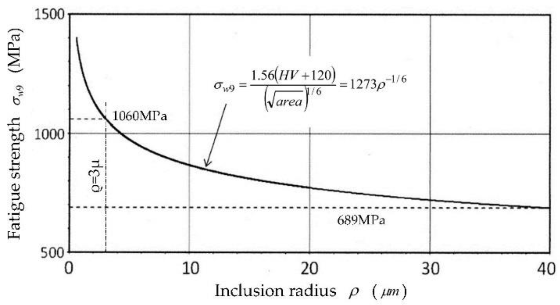
3.1. Effects of Size and Depth of Inclusions on the Fatigue Strength

According to the $\sqrt{area}$ model proposed by Y. Murakami [9], the fatigue limit of a metallic material, ${\sigma }_w$, was well provided by the defect size $\rho$ and the Vickers’ hardness HV (kgf/mm²), as follows;

$${\sigma }_w=\alpha \left(HV+120\right)/{\left(\sqrt{area}\right)}^{1/6},$$

(1)

where area indicates the area of the defect projected perpendicular to the longitudinal direction of the specimen, and the factor of $\alpha$ was given by $\alpha =1.43$ for surface defect and $\alpha =1.56$ for interior defect, respectively.

When this concept of $\sqrt{area}$ was applied to the fatigue strength at N = 10⁹ cycles as an attempt, assuming a spherical interior inclusion with a radius of $\rho$, the fatigue strength at N = 10⁹, ${\sigma }_{w9}$, was given by the following expression,

$${\sigma }_{w9}=1.56\left(HV+120\right)/{\left(\sqrt{\pi {\rho }^2}\right)}^{1/6}.$$

(2)

Since the Vickers’ hardness of this bearing steel (JIS:SUJ2) was reported as HV = 778 [3], Equation (2) was reduced as follows;

$${\sigma }_{w9}=1273{\rho }^{-1/6}$$

(3)

Equation (3) indicates the relationship between the fatigue strength at N = 10⁹ and the inclusion size (radius) for this steel.

Such a relationship is depicted in Figure 3. When the inclusion size is small, those inclusions have no harmful effect on the fatigue strength, as reported by many researchers [24,25]. From this point of view, if the critical small size is assumed as $\rho =3$ μm in this study, the upper bound of the fatigue strength given by Equation (3) becomes ${\sigma }_{w9}=1060 \mathrm{M}$Pa, as indicated in Figure 3. On the other hand, an inclusion larger than 40 μm ($\rho >40$ μm) is seldom found in the present steel. In such an assumption, the lower bound of the fatigue strength given by Equation (3) becomes ${\sigma }_{w9}=689 \mathrm{M}$Pa, as indicated by the horizontal dotted line in Figure 3. Thus, the distribution range of the fatigue strength at N = 10⁹ due to the distribution of the inclusion size would be 689 MPa~1060 MPa.

In the case of the rotating bending, the stress distribution across the specimen section has a distinct gradient, such that the stress on the surface gives the maximum and the stress becomes zero at the center of the section. Accordingly, the inclusion depth is another important factor to govern the fatigue strength of ${\sigma }_{w9}$, even if the inclusion size is fixed to a certain value. When the fatigue strength at the depth ξ is denoted as ${\sigma }_{w9}$, the fatigue strength evaluated by nominal bending stress on the specimen surface, ${\sigma }_{w9}^{*}$, is given as follows [26];

$${\sigma }_{w9}^{*}=\frac{r}{r-\xi }{\sigma }_{w9}=\frac{1.5}{1.5-\xi }{\sigma }_{w9}$$

(4)

where r indicates the radius of the critical portion of the specimen. Here, substituting Equation (3) into Equation (4), we have the following expression;

$${\sigma }_{w9}^{*}=\frac{1.5}{1.5-\xi }\times 1273{\rho }^{-1/6}=\frac{1910}{1.5-\xi }{\rho }^{-1/6}$$

(5)

Consequently, the fatigue strength of ${\sigma }_{w9}^{*}$ for the specimen with an inclusion size of $\rho$ and a depth of ξ could be calculated by Equation (5).

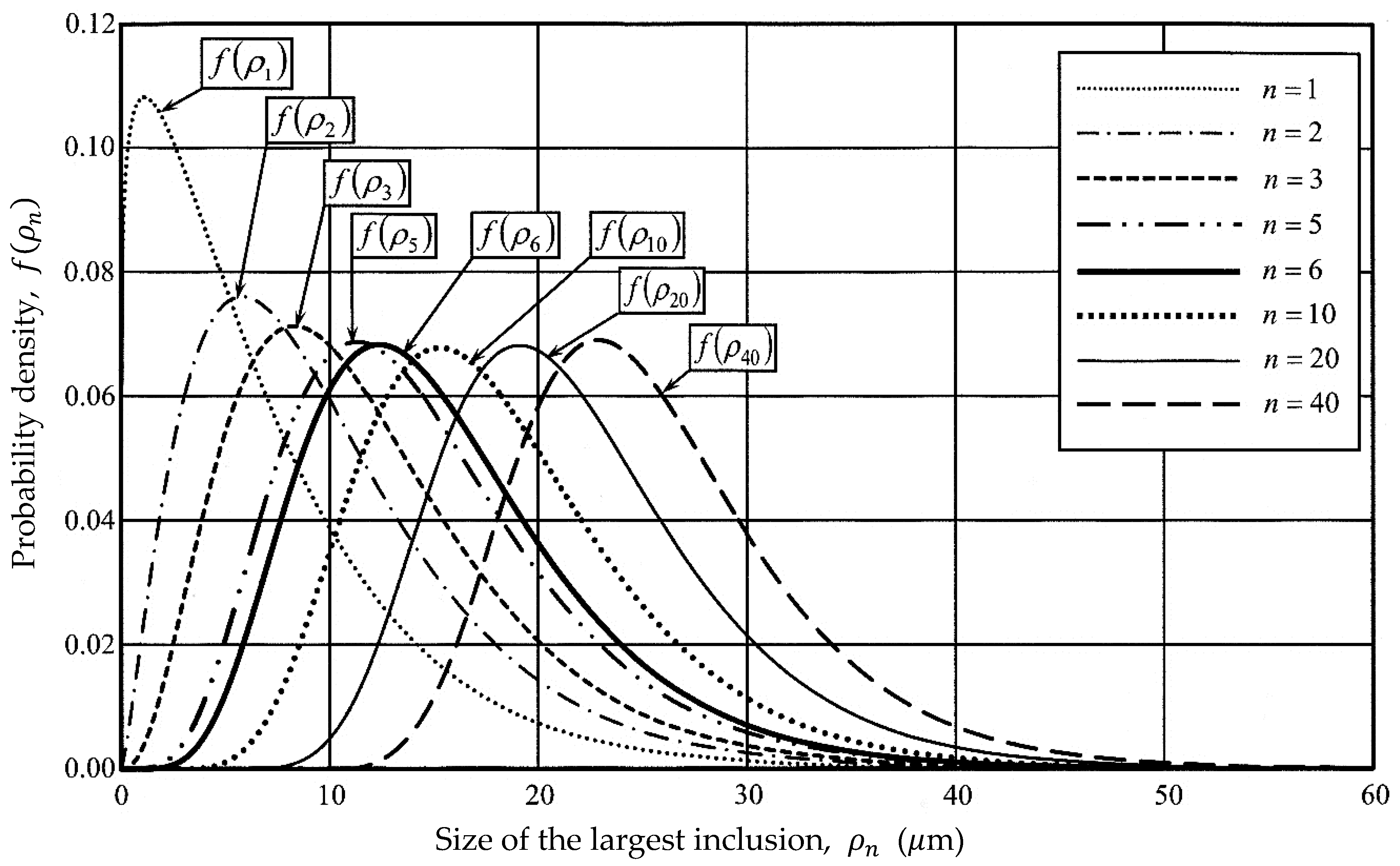
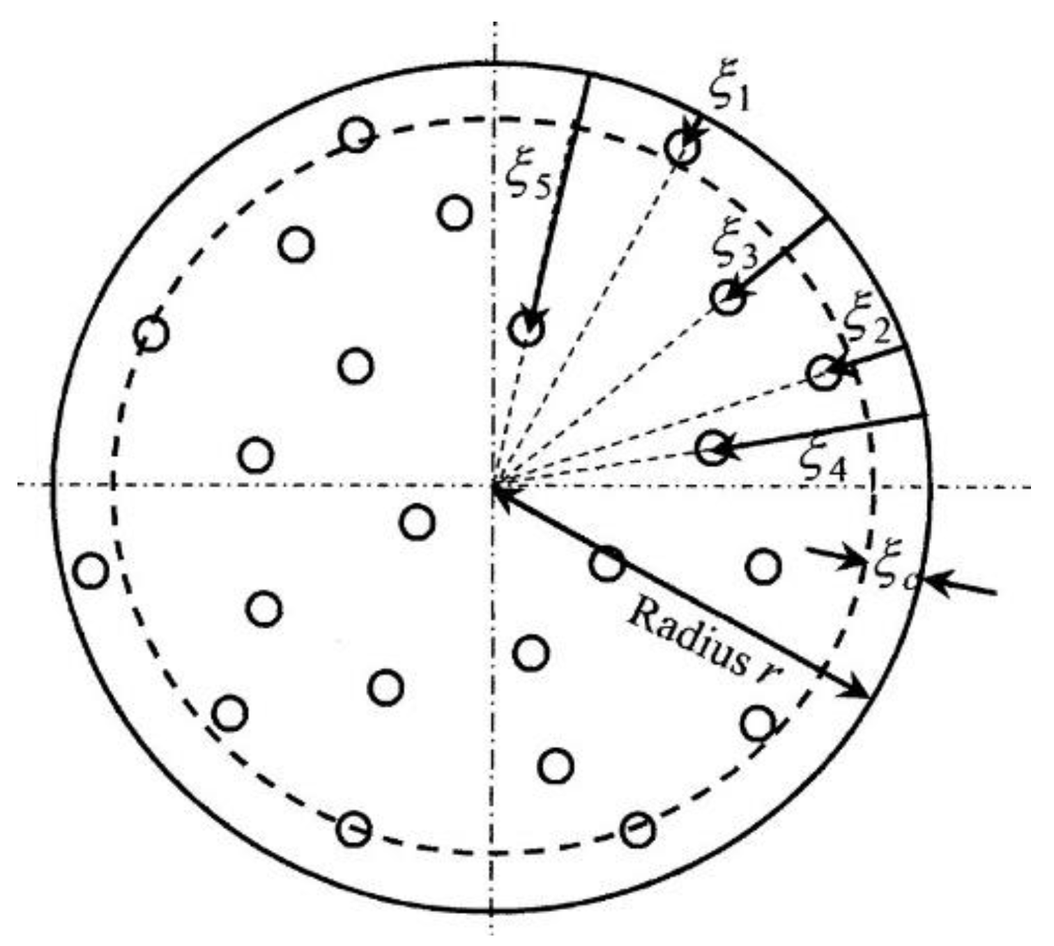
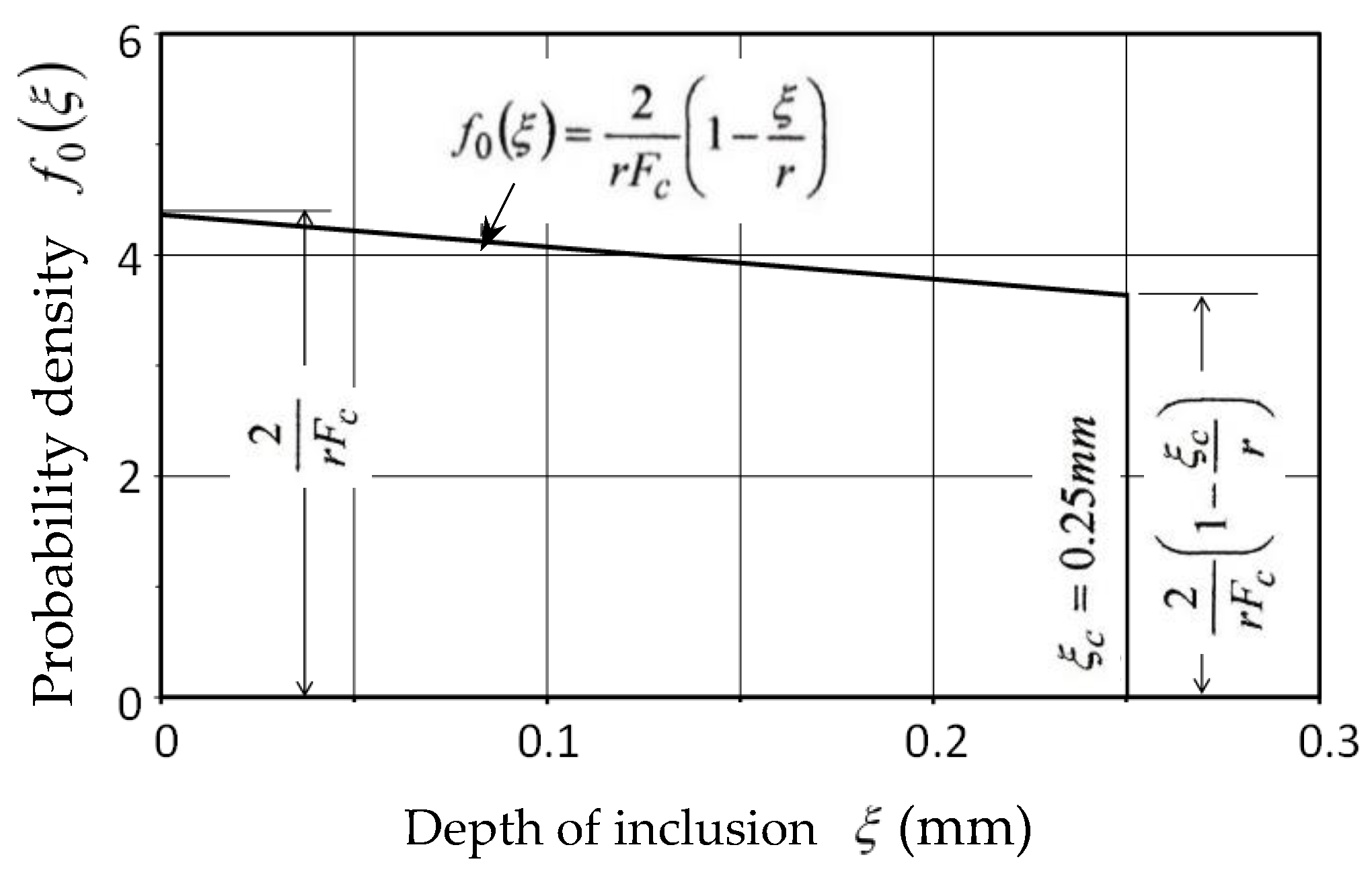
3.2. Distribution Characteristics of Inclusion Size and Inclusion Depth

The inclusion size is not constant, and therefore, the size has its own distribution characteristics peculiar to the fabrication process of the metallic material [11,12,13]. Of course, since the inclusion size $\rho$ is always positive, we have $\rho >0$. In other words, the lower bound of the inclusion size is assumed “0”. In addition, a size larger than 40 μm is seldom found in the bearing steel. Distribution pattern of the inclusion size with the above feature is well-represented by a two-parameter Weibull distribution [27], without a location parameter. The probability density function and the cumulative distribution function are given as follows:

$$f_0\left(\rho \right)=\frac{a}{b}{\left(\frac{\rho }{b}\right)}^{a-1}exp\left\{-{\left(\frac{\rho }{b}\right)}^a\right\},$$

(6)

and

$$F_0\left(\rho \right)=1-exp\left\{-{\left(\frac{\rho }{b}\right)}^a\right\},$$

(7)

where a is the shape parameter and b is the scale parameter, respectively.

When the number of inclusions included within the critical volume of a specimen is denoted by n, the inclusion with the maximum size would be the crack starter under the cyclic loadings. Accordingly, the distribution characteristics of the maximum size among n of inclusions in the critical volume become the most important factor to control the fatigue strength and fatigue life of the metallic material. Based on the concept of extremes’ distribution [28], the probability density function of the maximum size among n inclusions, $f\left({\rho }_n\right)$, is provided by

$$f\left({\rho }_n\right)=n{\left\{F_0\left({\rho }_n\right)\right\}}^{n-1}\frac{a}{b}{\left(\frac{{\rho }_n}{b}\right)}^{a-1}exp\left\{-{\left(\frac{{\rho }_n}{b}\right)}^a\right\}$$

(8)

Although we have to know the original distribution of the inclusion size $\rho$ itself, it is difficult to directly observe such a distribution pattern. In such a circumstance, the authors determined the respective parameters of the original size distribution, so as to satisfy the following conditions:

$$P\left[1 \mathsf{\mu }\mathrm{m}<\rho <15 \mathsf{\mu }\mathrm{m}\right]=0.8,F_0=0.1\mathrm{at}\rho =1 \mathsf{\mu }\mathrm{m}\mathrm{and}{F}_0=0.9\mathrm{at}\rho =15 \mathsf{\mu }\mathrm{m}.$$

This condition for the inclusion size was introduced here as a possible assumption supposed from the observation results by Toriyama et al. [12]. Thus, we obtain the results for the Weibull parameters as $a=1.139$ and $b=7.214$, respectively. In addition, since the number of inclusions inside the critical volume, n, is also unknown, the authors analyzed the distribution of the extremes by supposing various values as the number of inclusions, like n = 2, 3, 5, 6, 10, 20, and 40, respectively. Probability density functions of the maximum inclusion size thus calculated by Equation (8) are depicted in Figure 4, where $f\left({\rho }_1\right)$ plotted by a fine dotted curve in the most left hand side indicates the original probability density function of the inclusion size. The mode of the largest inclusion size, i.e., the inclusion size at each peak of the probability density function, tends to shift into the right hand side, with an increase in the number of inclusions in the critical volume of the specimen.

As described in Section 3.1, the inclusion depth at the crack initiation site, ξ, plays an important role to control both the fatigue strength and fatigue life of the metallic material, in the case of the rotating bending, due to the steep slope of the stress distribution across the section. Figure 5 indicates the distribution feature of the inclusions projected to the specimen section, assuming random distribution (uniform distribution) [23]. Here, if the inclusion depth from the surface is denoted as ${\xi }_1$, ${\xi }_2$, …, ${\xi }_n$, from the most shallow inclusion, one can obtain the one-dimensional distribution of the inclusion depth. As reported in another paper [26], the probability density function of the inclusion depth ξ can be represented by the following expression:

$$f\left(\xi \right)=\frac{2}{r}\left(1-\frac{\xi }{r}\right),[0<\xi <r].$$

(9)

In Equation (9), r indicates the radius of the specimen. The probability density of Equation (9) becomes a maximum at the specimen surface (ξ = 0), whereas the density becomes zero at the center of the specimen section. As reported by several researchers [5,29], the depth of the crack initiation site is restricted within the thin surface layer of ξ < 250$\mathsf{\mu }\mathrm{m}$ in rotating bending. Therefore, the probability density function of Equation (9) should be normalized as the conditional distribution, under the condition of ξ < 250$\mathsf{\mu }\mathrm{m}$. Thus, we have the actual probability density function of ξ, as follows:

$$f_0\left(\xi \right)=\frac{2}{r{F}_c}\left(1-\frac{\xi }{r}\right),[0<\xi <250 \mathsf{\mu }\mathrm{m}],$$

(10)

where $F_c$ indicates the probability giving the condition of $0<\xi <250 \mathsf{\mu }\mathrm{m}$ and its probability becomes $F_c=0.3055$ in the condition of the present work. The probability density function thus normalized by Equation (10) is depicted in Figure 6.

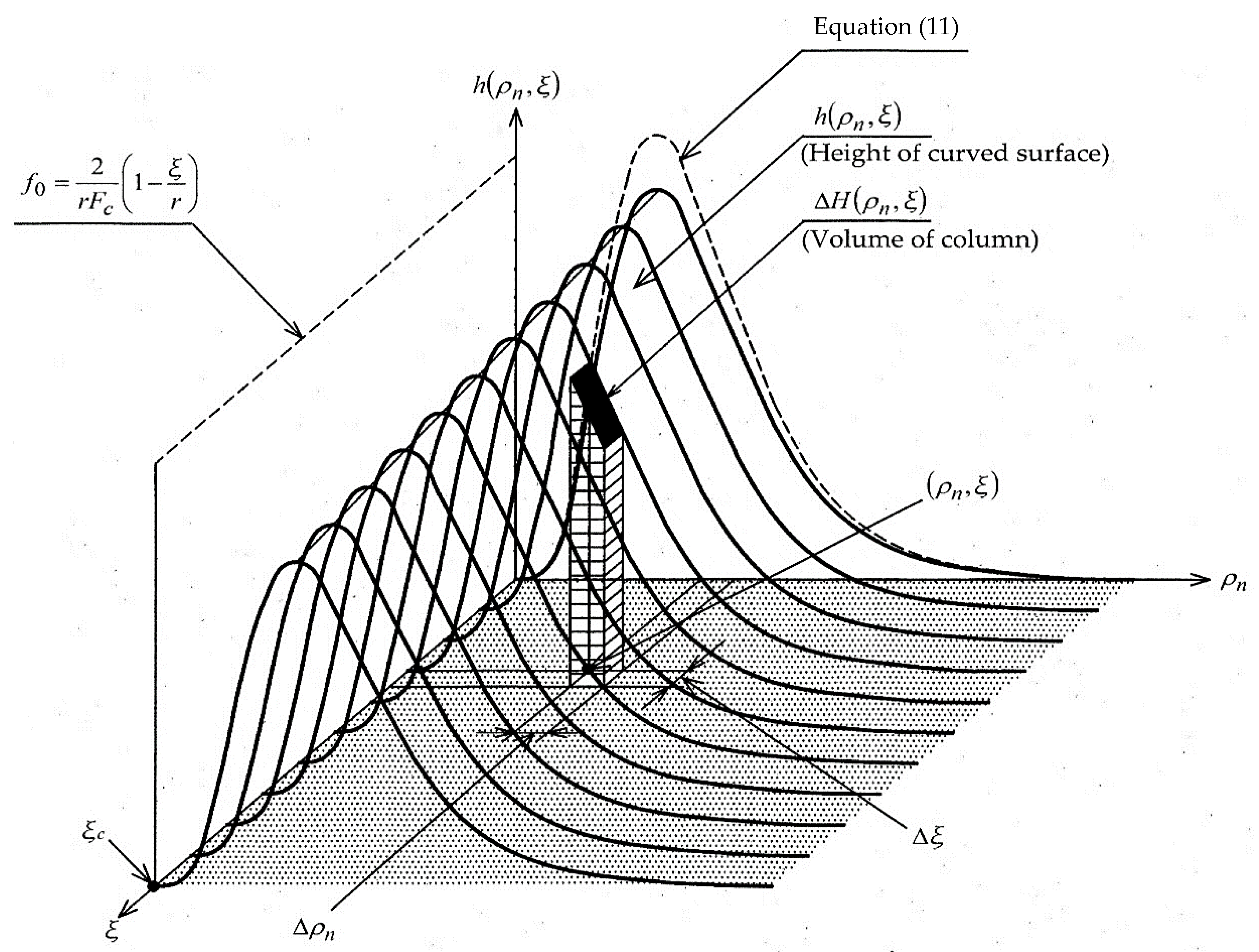
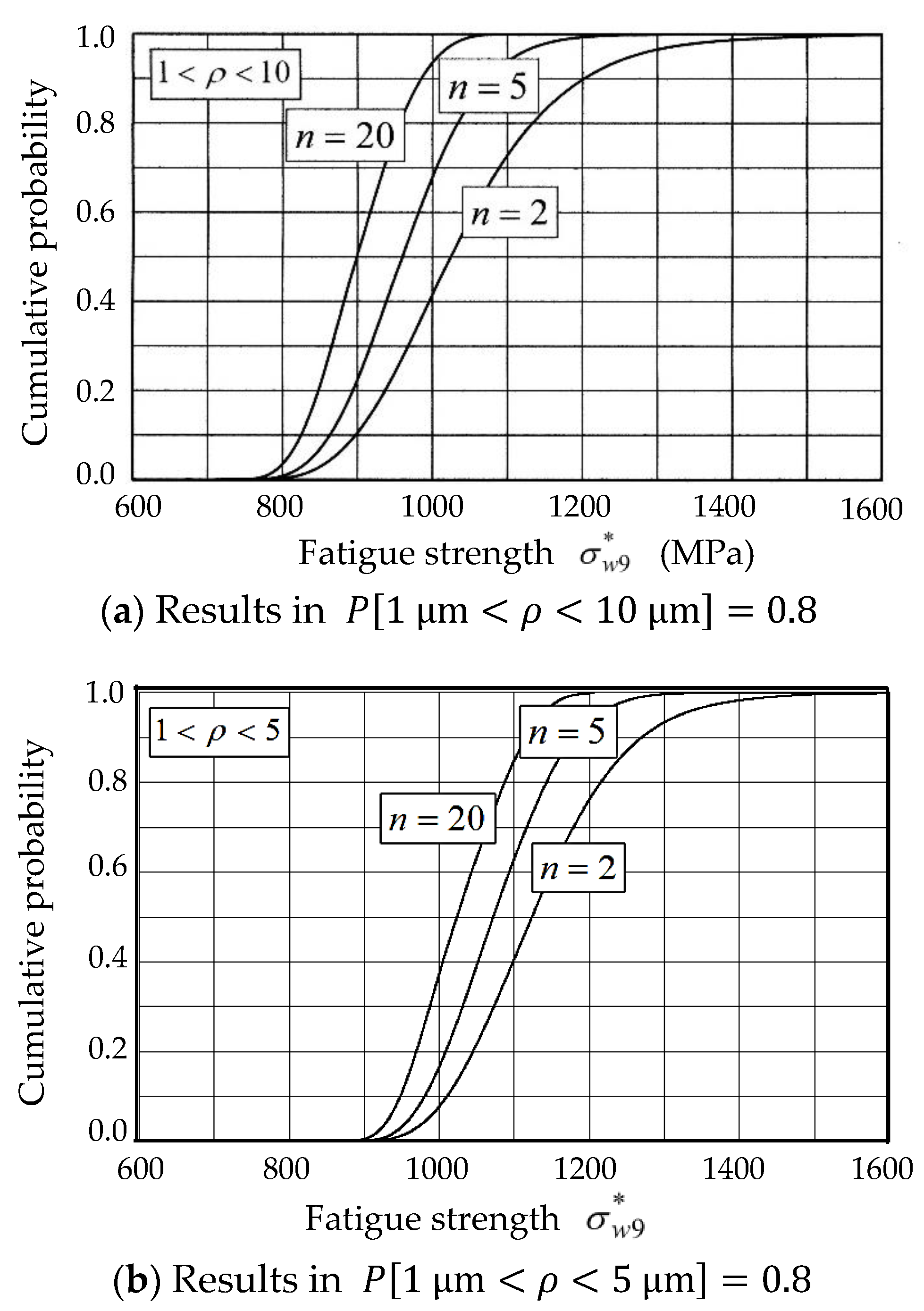
3.3. Joint Distribution of Inclusion Size and Inclusion Depth and Analysis of Fatigue Strength Distribution

In the previous section, distribution characteristics on the size and the depth of the inclusion are discussed, and the probability density functions of $f\left({\rho }_n\right)$ and $f_0\left(\xi \right)$ are derived as Equations (8) and (10). Since both ${\rho }_n$ and ξ are statistically independent random variables, the joint probability density function, $h\left({\rho }_n,\xi \right)$, is given by

$$h\left({\rho }_n,\xi \right)=f\left({\rho }_n\right)·f_0\left(\xi \right)= n{\left\{F_0\left({\rho }_n\right)\right\}}^{n-1}\frac{a}{b}{\left(\frac{{\rho }_n}{b}\right)}^{a-1}exp\left\{-{\left(\frac{{\rho }_n}{b}\right)}^a\right\}·\frac{2}{r{F}_c}\left(1-\frac{\xi }{r}\right)$$

(11)

By putting n = 5, $a=1.139$, $b=7.214$, r = 1.5, and $F_c=0.3055$ along the previous example, the joint probability density function of $h\left({\rho }_n,\xi \right)$ was numerically calculated. The result of $h\left({\rho }_n,\xi \right)$ thus obtained is depicted in Figure 7, where the joint probability function of $h\left({\rho }_n,\xi \right)$ gives the curved surface like a mountain range. In the figure, $\Delta H\left({\rho }_n,\xi \right)$ corresponding to the volume of the vertical column indicates the probability that ${\rho }_n$ and $\xi$ are within the square region of $\Delta {\rho }_n\times \Delta \xi$. The dashed line appearing on the $\xi -h\left({\rho }_n,\xi \right)$ plane corresponds to the marginal distribution for the inclusion depth $\xi$, as given by Equation (10). On the other hand, another dashed curve appearing on the ${\rho }_n-h\left({\rho }_n,\xi \right)$ plane corresponds to the marginal distribution for the inclusion size of ${\rho }_n$, given by Equation (12).

$$f\left({\rho }_n\right)=\underset{0}{\overset{{\xi }_c}{{\displaystyle \int }}}h\left({\rho }_n,\xi \right)d\xi =n{\left\{F_0\left({\rho }_n\right)\right\}}^{n-1}\frac{a}{b}{\left(\frac{{\rho }_n}{b}\right)}^{a-1}exp\left\{-{\left(\frac{{\rho }_n}{b}\right)}^a\right\}$$

(12)

In this place, let us divide the ${\rho }_n-\xi$ plane into fine meshes of $\Delta {\rho }_n\times \Delta \xi$ and consider the mesh at the arbitrary point of $\left({\rho }_n,\xi \right)$, as shown in Figure 7. Then, the probability that the inclusion size ${\rho }_n$ and the inclusion depth $\xi$ yield within the area of $\Delta {\rho }_n\times \Delta \xi$ is provided by the volume of the vertical column raising at this mesh of $\Delta {\rho }_n\times \Delta \xi$. In other words, the volume of this column corresponds to the probability that the fatigue strength at N = 10⁹ is given by Equation (5). Thus, we have the following equation,

$$P\left[{\rho }_n\in \Delta {\rho }_n{\displaystyle \cap }\xi \in \Delta \xi \right]=h\left({\rho }_n,\xi \right)\Delta {\rho }_n\Delta \xi =P\left[{\sigma }_{w9}^{*}\in \Delta {\sigma }_{w9}^{*}\right]$$

(13)

Based on the repetition of numerical calculations by Equation (13), the probability density function $f\left({\sigma }_{w9}^{*}\right)$ and the cumulative distribution function $F\left({\sigma }_{w9}^{*}\right)$ can be analyzed numerically.

4. Results and Discussions

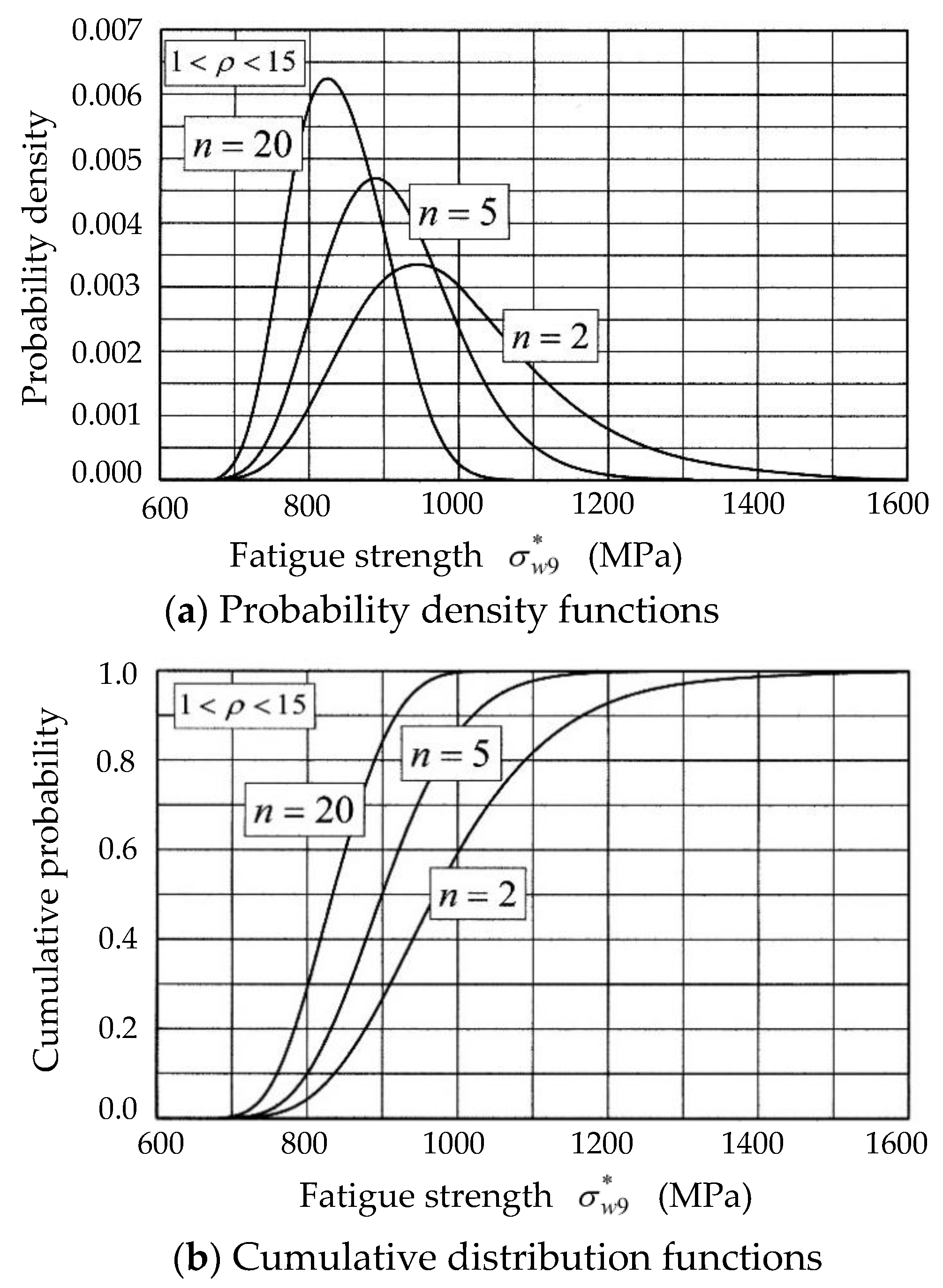
4.1. Distribution Characteristics of Fatigue Strength ${\sigma }_{w9}^{*}$

Since the number of inclusions included within the critical volume of a specimen is unknown, the authors analyzed the distribution characteristics of the fatigue strength, ${\sigma }_{w9}^{*}$, assuming several numbers of inclusions like n = 2, 3, 5, 6, 10, 20, and 40, respectively. Among them, the analytical results of the fatigue strength distribution obtained for n = 2, 5, and 20, by the method in the previous section are indicated in Figure 8 as typical examples. Figure 8a shows the probability density functions under these three cases of n = 2, 5, and 20, whereas Figure 8b indicates the cumulative distribution functions corresponding to the respective cases. Weibull parameters a and b in Equation (8) are provided to satisfy the condition of $P\left[1 \mathsf{\mu }\mathrm{m}<\rho <15 \mathsf{\mu }\mathrm{m}\right]=0.8$. It is found that the peak (mode) and the standard deviation of the fatigue strength distribution tends to decrease with an increase in the inclusion number.

In order to investigate the effect of the condition for the dispersion of the inclusion size of $\rho$, similar analyses were performed, giving some other conditions of $P\left[1 \mathsf{\mu }\mathrm{m}<\rho <10 \mathsf{\mu }\mathrm{m}\right]=0.8$ and $P\left[1 \mathsf{\mu }\mathrm{m}<\rho <5 \mathsf{\mu }\mathrm{m}\right]=0.8$. Among these analyses, only the results of the cumulative distribution functions are indicated in Figure 9, due to article page limit. As seen in Figure 8b and Figure 9, median of the fatigue strength distribution tends to increase with a decrease of the dispersion of the inclusion size, while standard deviation of the fatigue strength distribution tends to decrease a little, depending on the decrease of the dispersion of the inclusion size.

Comparing these analytical distribution characteristics of the fatigue strength ${\sigma }_{w9}^{*}$ in Figure 8 and Figure 9 with the experimental result in Figure 1, the distribution feature of the fatigue strength ${\sigma }_{w9}^{*}$ under the conditions of $P\left[1\mathsf{\mu }\mathrm{m}<\rho <15 \mathsf{\mu }\mathrm{m}\right]=0.8$ and n = 5 was roughly in agreement with the experimental distribution aspect of the fatigue strength at N = 10⁹. The most preferable number of inclusions, n, is further discussed again in Section 4.4.

4.2. Expansion of the Probabilistic Model to Analyze P-S-N Characteristics in Interior-Induced Fracture

Target of the probabilistic model described in Section 3 is the distribution characteristics of the fatigue strength only at stress cycles of N = 10⁹. Accordingly, the analytical model should be conceptionally expanded to interpret the whole statistical aspect of the S-N property, in the interior inclusion-induced fracture mode. From this point of view, denoting the fatigue strength at any stress cycle, $N_{fix}$, by ${\sigma }_w$, Equation (3) is rewritten as follows:

$${\sigma }_w=1273·{\rho }^{-1/6}+\beta ,$$

(14)

$$\beta =\lambda \left\{log\left(N_{fix}\right)\right\}+\gamma .$$

(15)

Based on the dotted S-N curve in Figure 1, parameters λ and γ in Equation (15) were determined from two points $\left(N={10}^6, {\sigma }_{w9}^{*}=1424 \mathrm{MPa} \right)$ and $\left(N={10}^9, {\sigma }_{w9}^{*}=920 \mathrm{MPa} \right)$ as λ = −168 and γ = 1512, respectively. Substituting these values into Equations (14) and (15), Equation (14) is rewritten as

$${\sigma }_w=1273·{\rho }^{-1/6}-168·\left\{log\left(N_{fix}\right)\right\}+1512.$$

(16)

Here, ${\sigma }_w-\rho$ relationships under the fixed numbers of the fatigue life of N = 10⁶, N = 10⁷, N = 10⁸, and N = 10⁹ are depicted in Figure 10. As suggested from Equations (14)–(16), analytical curves in Figure 10 tend to shift in parallel along the ordinate. Of course, the curve tends to shift downwards with an increase in the fixed number of stress cycles. Applying the concept of Equation (4), one could calculate the fatigue strength ${\sigma }_w^{*}$ by

$${\sigma }_w^{*}=\frac{1.5}{1.5-\xi }\left[1273·{\rho }^{-1/6}-168·\left\{log\left(N_{fix}\right)\right\}+1512\right].$$

(17)

Equation (17) includes arbitrarily given number of stress cycles $N_{fix}$, together with the inclusion size $\rho$ and the inclusion depth ξ. Therefore, combining the joint probability function in Figure 7 with Equation (17), one could analyze the distribution characteristics of the fatigue strength at any number of stress cycles $N_{fix}$ by repeating the numerical calculations.

Probability density functions of the fatigue strength thus obtained at N = 10⁶, 10⁷, 10⁸, and 10⁹ are indicated at the respective numbers of the stress cycles in Figure 11. These analytical results are roughly in agreement with the overall feature of the experimental aspect on the statistical fatigue characteristics. The scale of the axis for the probability density is adjusted to correspond to each value listed in the table attached in the right-hand side in Figure 11. The percentile points of $F=1\%$, 10%, 50%, 90%, and 99% for the fatigue strength are indicated by marks of ◇’s along the vertical axis of the probability density functions. The respective thin dotted lines passing through the percentile points corresponding to the same probability give the P-S-N curves representing the statistical fatigue characteristics of this steel. All data points yield within the range of 1–99% in Figure 11. This fact suggests that the probabilistic model developed in this study has an availability to interpret the physical meaning of the statistical fatigue property in the very high cycle regime.

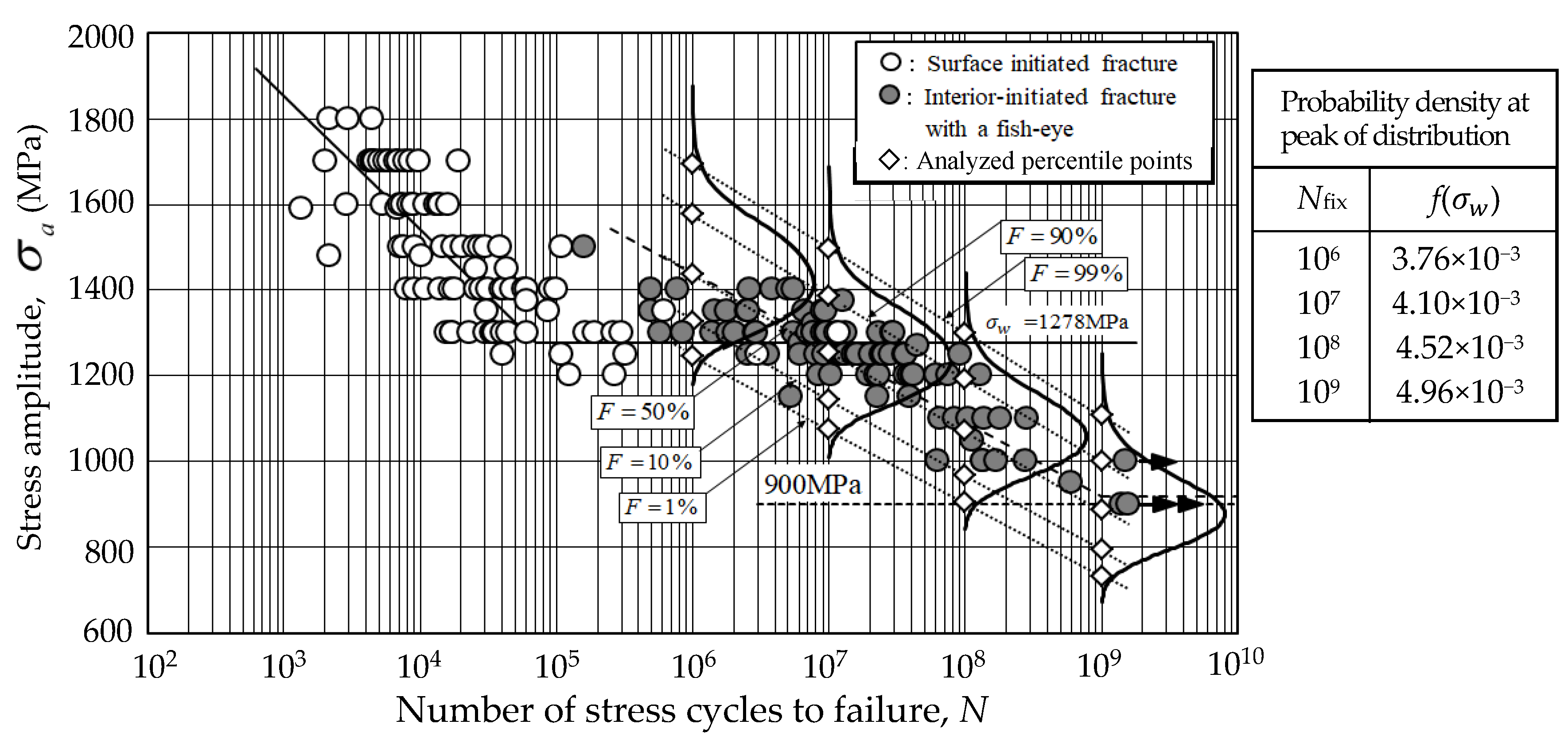
4.3. Analysis of the Fatigue Life Distributions in Interior-Induced Fracture Mode

Although distribution characteristics of the fatigue strength ${\sigma }_w^{*}$ at the given number of stress cycles were analyzed in the previous section, the fatigue life distributions could also be analyzed based on Equation (17), by giving any value of the stress amplitude ${\sigma }_w^{*}$. Applying this method, fatigue life distributions were calculated at ${\sigma }_w^{*}$ = 1400 MPa, 1200 MPa, 1000 MPa, and 900 MPa, respectively. The probability density functions thus obtained were indicated at the respective stress levels in Figure 12. Since the fatigue life increased logarithmically with decrease of the stress level, the probability density at the peak of the density function tended to decrease such that the integrated value of the density function maintained unity. Values of the peak density at the respective stress levels are indicated on the right-hand side, in Figure 12. As shown in this table, the peak density varied drastically, depending on the stress level, due to the above described reason, but the distribution curves were drowned when they had the same height for the sake of convenience.

In order to distinguish the fatigue strength distribution and the fatigue life distribution, the notations of $f\left({\sigma }_w\right)$ and $F\left({\sigma }_w\right)$ are used for the fatigue strength distribution, whereas other notations of $g\left({\sigma }_w\right)$ and $G\left({\sigma }_w\right)$ are accepted for the fatigue life distribution. Similar to Figure 11, the percentile points of $G=1\%$, 10%, 50%, 90%, and 99% for the fatigue life are indicated by marks of ◇’s along the horizontal lines, at the respective stress levels. The respective thin dotted lines passing through the percentile points corresponding to the same probability give the P-S-N curves of this steel. All experimental data in the interior-induced fracture appear within the range of 1–99% in Figure 12. Thus, it was finally noted that the statistical fatigue property in the interior-induced fracture of this steel could be well explained from either one of the fatigue strength distribution and the fatigue life distribution, through the probabilistic model proposed in this study.

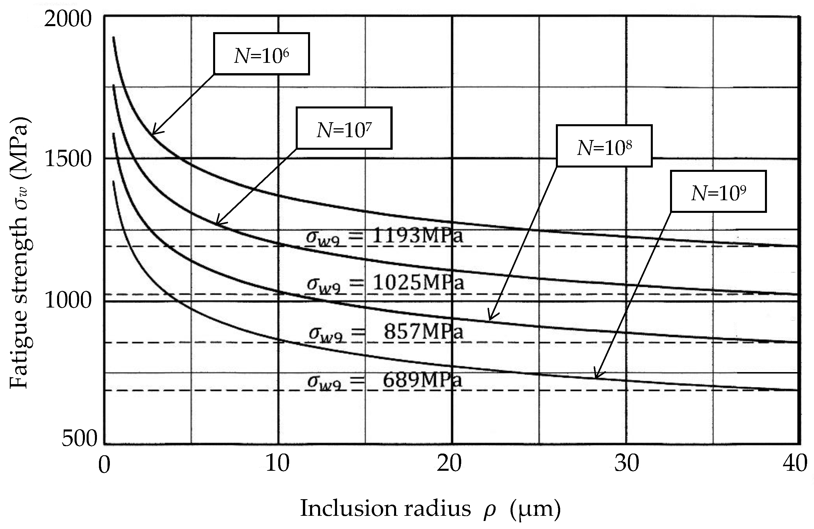
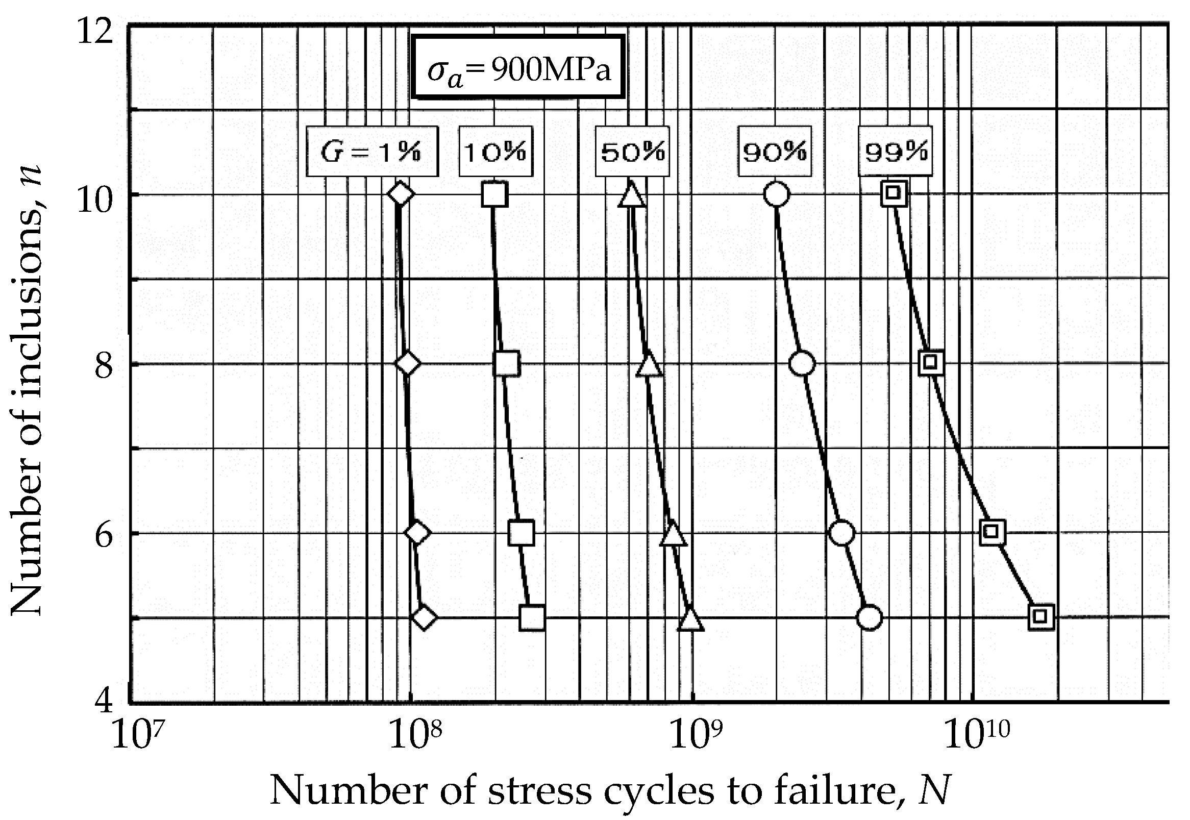
4.4. Reconfirmation of the Number of Inclusions in the Critical Volume

As described in Section 4.1, since the number of inclusions included in the critical volume is unknown, the analysis was carried out by setting three conditions of n = 2, 5, and 20, as the inclusion number. Then, the condition of n = 5 was tentatively selected as a preferable number of inclusions. However, in order to confirm the most reasonable number of inclusions, the fatigue life distributions were additionally analyzed, under conditions of n = 6, 8, and 10, respectively. Based on the series of analytical results, percentile points of the fatigue life distribution corresponding to $G=1\%$, 10%, 50%, 90%, and 99% were determined; the relationship between those percentile points and the number of inclusions are depicted in Figure 13. Comparing five solid curves carefully with the dispersion aspect of the experimental results in an interior-induced fracture in Figure 12, it was finally noted that the analytical result at n = 6 was well fitted compared to the result at n = 5.

Based on this evidence, the statistical fatigue properties (P-S-N properties) in Figure 11 and Figure 12 were numerically analyzed by putting n = 6 for the number of inclusions included in the critical volume of the specimen.

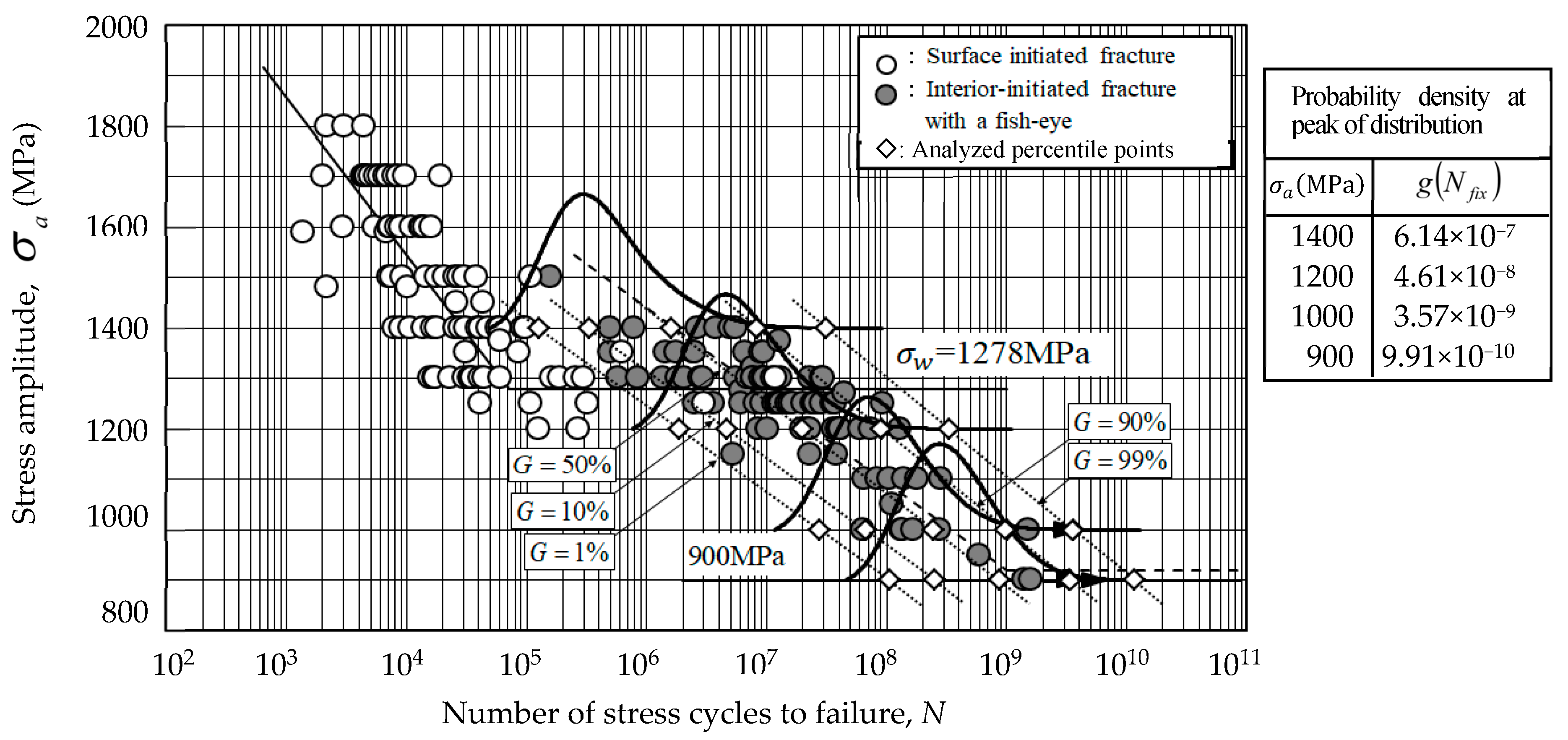
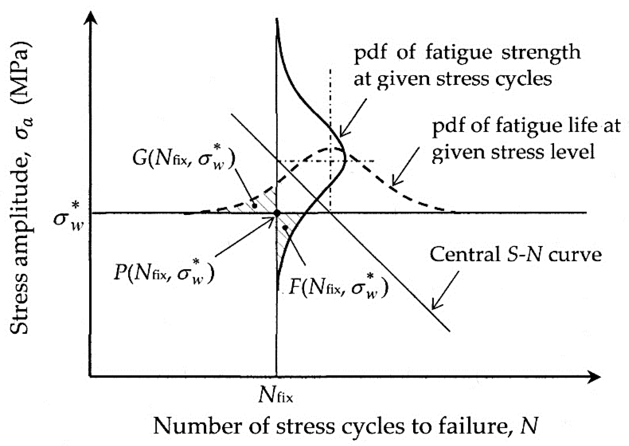
4.5. Mutual Relationship between Both Distributions of Fatigue Strength and Fatigue Life

In this study, the authors showed that both fatigue strength distribution and fatigue life distribution could be derived from the joint probability density function of $h\left({\rho }_n,\xi \right)$, given by Equation (11). It was also confirmed that the analytical results were in good agreement with the statistical aspect of the experimental fatigue data in the very high cycle regime. In this place, mutual relationship between the distribution aspects of the fatigue strength and the fatigue life is further discussed to reconfirm the reasonability of the present probabilistic model for the P-S-N characteristics. The mutual relationship between both distributions is illustrated in Figure 14, where the ordinate is the fatigue strength ${\sigma }_w^{*}$ and the abscissa is the fatigue life N. When any point P(N_fix, ${\sigma }_w^{*}$) is taken in this diagram, the probability that the fatigue life at the stress level ${\sigma }_w^{*}$ is less than N_fix always corresponds to the probability that the fatigue strength at the definite stress cycles N_fix is lower than ${\sigma }_w^{*}$. In other words, the cumulative probability of N_fix, G(N_fix,${\sigma }_w^{*}$), always corresponds to the cumulative probability of ${\sigma }_w^{*}$, F(N_fix,${\sigma }_w^{*}$) [30]. G(N_fix,${\sigma }_w^{*}$) gives the distribution function of the fatigue life at ${\sigma }_w^{*}$ and F(N_fix,${\sigma }_w^{*}$) gives the distribution function of the fatigue strength at N_fix. Thus, we have

$$G(N_{\mathrm{fix}},{\sigma }_w^{*})=F(N_{\mathrm{fix}},{\sigma }_w^{*})$$

(18)

Equation (18) implies that the dashed area G(N_fix,${\sigma }_w^{*}$) is always equal to the other dashed area F(N_fix,${\sigma }_w^{*}$) in Figure 14.

Based on this equality of Equation (18), one could obtain the S-N curve corresponding to any level of the fracture probability. Thus, the probabilistic S-N curves at the respective fracture probabilities could be analyzed as P-S-N curves. As described in Section 4.2 and Section 4.3, the distribution characteristics of the experimental S-N data were well explained from either viewpoint of the fatigue strength distribution or the fatigue life distribution. The equality of Equation (18) is the reason why the reasonable P-S-N curves could be equally obtained from different viewpoints of the fatigue strength distribution and the fatigue life distribution.

5. Conclusions

Main conclusions obtained in this study are summarized as follows.

1.

The probability density functions of the inclusion size at the crack initiation site, $f\left({\rho }_n\right)$, was successfully derived by combining the Weibull distribution and the concept of extreme distribution. In addition, the probability density function of the inclusion depth, $f_0\left(\xi \right)$, was also derived from the uniform distribution of the location of the inclusion in the material space.

2.

Since the inclusion size ${\rho }_n$ and the crack depth ξ are statistically independent, the joint probability density function of these random variables, $h\left({\rho }_n,\xi \right)$, is given by the direct multiplication of the above two probability density functions, such as $h\left({\rho }_n,\xi \right)=f\left({\rho }_n\right)·f_0\left(\xi \right)$.

3.

For the hourglass type specimen of a bearing steel with the definite hardness, the rotating bending fatigue strength of the specimen with any size $\rho$ and depth ξ of the inclusion at the arbitrarily given number of stress cycles N_fix is analytically provided in the very high cycle regime.

4.

Based on the above joint probability density function of $h\left({\rho }_n,\xi \right)$, repeating the numerical calculations following $P\left[{\rho }_n\in \Delta {\rho }_n{\displaystyle \cap }\xi \in \Delta \xi \right]=h\left({\rho }_n,\xi \right)\Delta {\rho }_n\Delta \xi =P\left[{\sigma }_{w9}^{*}\in \Delta {\sigma }_{w9}^{*}\right]$, one could obtain the fatigue strength distribution at any number of stress cycles and the fatigue life distribution at any stress level. The analytical results thus obtained were in good agreement with the statistical feature of the experimental fatigue test data.

In the construction of the probabilistic model in this study, several assumptions were introduced for the sake of simplicity. In order to reconfirm the reasonability of such assumptions, sufficient number of experimental results should be further filed up in the future. In addition, it is still unknown whether the fatigue limit exists for the interior inclusion-induced fracture mode. This is one of the most important issues to be solved in the near future.

References

1. Bathias, C. There is no infinite fatigue life in metallic materials. Fatigue Fract. Eng. Mater. Struct. 1999, 22, 559–565. [Google Scholar] [CrossRef]
2. Mughrabi, H. Specific features and mechanisms of fatigue in the ultrahigh-cycle regime. Int. J. Fatigue 2006, 28, 1501–1508. [Google Scholar] [CrossRef]
3. Sakai, T.; Takeda, M.; Shiozawa, K.; Ochi, Y.; Nakajima, M.; Nakamura, T.; Oguma, N. Experimental reconfirmation of characteristic S-N property for high carbon chromium bearing steel in wide life region in rotating bending. J. Soc. Mat. Sci. Jpn. 2000, 49, 779–785. [Google Scholar] [CrossRef] [Green Version]
4. Bathias, C.; Paris, P.C. Gigacycle Fatigue in Mechanical Practice; Marcel Deckker: New York, NY, USA, 2005. [Google Scholar]
5. Sakai, T.; Sato, Y.; Oguma, N. Characteristic S-N properties of high-carbon-chromium-bearing steel under axial loading in long-life fatigue. Fatigue Fract. Eng. Mater. Struct. 2002, 25, 765–773. [Google Scholar] [CrossRef]
6. Sakai, T.; Sato, Y.; Nagano, Y.; Takeda, M.; Oguma, N. Effect of stress ratio on long life fatigue behavior of high carbon chromium bearing steel under axial loading. Int. J. Fatigue 2006, 28, 1547–1554. [Google Scholar] [CrossRef]
7. Sakai, T.; Lian, B.; Takeda, M.; Shiozawa, K.; Oguma, N.; Ochi, Y.; Nakajima, M.; Nakamura, T. Statistical duplex S-N characteristics of high carbon chromium bearing steel in rotating bending in very high cycle regime. Int. J. Fatigue 2010, 32, 497–504. [Google Scholar] [CrossRef]
8. Oguma, N.; Lian, B.; Sakai, T.; Watanabe, K.; Odake, Y. Long life fatigue fracture induced by interior inclusions for high carbon chromium bearing steels under rotating bending. J. ASTM Int. 2010, 7, 1–9. [Google Scholar] [CrossRef]
9. Murakami, Y. Metal Fatigue: Effects of Small Defects and Nonmetallic Inclusions; Elsevier: Oxford, UK, 2002; pp. 88–94. [Google Scholar]
10. Takeda, M.; Sakai, T.; Oguma, N. Rotating bending fatigue property and fractography for high strength steels and carbon steel over ultra wide life region. Trans. JSME Ser. A 2002, 68, 977–984. [Google Scholar] [CrossRef]
11. Murakami, Y.; Kodama, S.; Konuma, S. Quantitative evaluation of effects of nonmetallic inclusions on fatigue strength of high strength steel. Trans. JSME Ser. A 1988, 54, 688–696. [Google Scholar] [CrossRef] [Green Version]
12. Toriyama, T.; Murakami, Y.; Makino, T. Database of nonmetallic inclusions and its application to the fatigue strength prediction method of high strength steels. J. Soc. Mat. Sci. Jpn. 1991, 40, 1497–1503. [Google Scholar] [CrossRef] [Green Version]
13. Adachi, A.; Shoji, H.; Kuwabara, A.; Inoue, Y. Rotating bending fatigue phenomenon of JIS SUJ2 bearing steel. DENKI SEIKO 1975, 46, 176–182. [Google Scholar] [CrossRef]
14. Barbosa, J.F.; Correia, J.A.F.O.; Junior, R.C.S.F.; De Jesus, A.M.P. Fatigue life prediction of metallic materials considering mean stress effects by means of an artificial neural network. Int. J. Fatigue 2020, 135, 105527. [Google Scholar] [CrossRef]
15. Gope, P.C.; Mahar, C.S. Evaluation of fatigue damage parameters for Ni-based super alloys Inconel 825 steel notched specimen using stochastic approach. Fatigue Fract. Eng. Mater. Struct. 2021, 44, 427–443. [Google Scholar] [CrossRef]
16. Lehner, P.; Krejsa, M.; Parenica, P.; Krivy, V.; Brozovsky, J. Fatigue damage analysis of a riveted steel overhead crane support truss. Int. J. Fatigue 2019, 128, 105190. [Google Scholar] [CrossRef]
17. Tomaszewski, T.; Strzelecki, P.; Wachowski, M.; Stopel, M. Fatigue life prediction for acid-resistant steel plate under operating loads. Bull. Pol. Acad. Tech. 2020, 68, 913–921. [Google Scholar] [CrossRef]
18. Feng, L.; Zhang, L.; Liao, X.; Zhang, W. Probabilistic fatigue life of welded plate joints under uncertainty in arctic areas. J. Constr. Steel Res. 2021, 176, 106412. [Google Scholar] [CrossRef]
19. Caiza, P.D.T.; Ummenhofer, T. A probabilistic Stussi function for modelling the S-N curves and its application on specimens made of steel S355J2+N. Int. J. Fatigue 2018, 117, 121–134. [Google Scholar] [CrossRef]
20. Mughrabi, H. Zur Dauerschwingfestigkeit im Bereich extrem hoher bruchlastspielzahlen: Mehrstufige lebensdauerkurven. HTM/Harterei-Tech. Mitt. 2001, 56, 300–303. [Google Scholar]
21. Harlow, D.G.; Wei, R.P.; Sakai, T.; Oguma, N. Crack growth based probability modeling of S-N response for high strength steel. Int. J. of Fatigue 2006, 28, 1479–1485. [Google Scholar] [CrossRef]
22. Sakai, T. Chair of Editorial Committee. In Standard Evaluation Method of Fatigue Reliability for Metallic Materials—Standard Regression Method of S-N Curves; JSMS-SD-11-07; The Society of Materials Science: Kyoto, Japan, 2007. [Google Scholar]
23. Nakagawa, A.; Sakai, T.; Harlow, D.G.; Oguma, N.; Nakamura, Y.; Ueno, A.; Kikuchi, S.; Sakaida, A. A probabilistic model on crack initiation modes of metallic materials in very high cycle fatigue. Procedia Struct. Integr. 2016, 2, 1199–1206. [Google Scholar] [CrossRef]
24. Kitagawa, H.; Takahashi, S. Fracture mechanics study on small fatigue crack growth and the condition of its threshold. Trans. JSME Ser. A 1979, 45, 1289–1303. [Google Scholar]
25. Tanaka, K.; Nakai, Y.; Yamashita, M. Fatigue growth threshold of small cracks. Int. J. Fract. 1981, 17, 519–533. [Google Scholar]
26. Nakamura, Y.; Sakai, T.; Harlow, D.G.; Oguma, N.; Nakajima, M.; Nakagawa, A. Probabilistic model on statistical fatigue property in very high cycle regime based on distributions of size and location of interior inclusions. In Proceedings of the VHCF-7, Dresden, Germany, 3–5 July 2017; pp. 81–86. [Google Scholar]
27. Weibull, W. A statistical distribution function of wide applicability. J. Appl. Mech. 1951, 18, 293–297. [Google Scholar]
28. Gumbel, E.J. Statistics of Extremes; Columbia University Press: New York, NY, USA, 1958; pp. 75–78. [Google Scholar]
29. Shiozawa, K.; Lu, L.-T.; Ishihara, S. Subsurface fatigue crack initiation behavior and S-N curve characteristics in high carbon-chromium bearing steel. J. Soc. Mat. Sci. Jpn. 1999, 48, 1095–1100. [Google Scholar] [CrossRef] [Green Version]
30. Sakai, T.; Sakaida, A.; Fujitani, K.; Tanaka, T. A study on statistical fatigue properties of metallic materials with particular attention to relation between fatigue life and fatigue strength distributions. Mem. Res. Inst. Sci. Eng. 1982, 42, 79–91. [Google Scholar]
Figure 1. Rotating bending S-N characteristics of bearing steel in very high cycle regime.
Applsci 11 02889 g001
Figure 2. SEM observations of fracture surfaces in surface-induced fracture and interior inclusion-induced fracture.
Applsci 11 02889 g002
Figure 3. Relationship between fatigue strength σ w 9 and inclusion radius ρ .
Applsci 11 02889 g003
Figure 4. Probability density functions of the largest inclusion size among various numbers of inclusions.
Applsci 11 02889 g004
Figure 5. Definition of inclusion depth from surface.
Applsci 11 02889 g005
Figure 6. Probability function of inclusion depth f 0 ( ξ ) .
Applsci 11 02889 g006
Figure 7. Schematics of joint probability density function of ρ n and ξ .
Applsci 11 02889 g007
Figure 8. Distribution patterns of fatigue strength.
Applsci 11 02889 g008
Figure 9. Comparison of cumulative distribution functions in respective conditions.
Applsci 11 02889 g009
Figure 10. σw-   ρ relationships at several given numbers of stress cycles.
Applsci 11 02889 g010
Figure 11. Fatigue strength distributions and P-S-N curves in very high cycle regime.
Applsci 11 02889 g011
Figure 12. Fatigue life distributions and P-S-N curves in a very high cycle regime.
Applsci 11 02889 g012
Figure 13. Number of inclusions versus number of stress cycles to failure.
Applsci 11 02889 g013
Figure 14. Relationship between fatigue strength distribution and fatigue life distribution.
Applsci 11 02889 g014