Identifying Changes in Sediment Texture along an Ephemeral Gravel-Bed Stream Using Electrical Resistivity Tomography 2D and 3D

Abstract

Differences in deposit geometry and texture with depth along ephemeral gravel-bed streams strongly reflect fluctuations in bedload which are due to environmental changes at the basin scale and to morphological channel adjustments. This study combines electrical resistivity tomography (ERT) with datasets from borehole logs to analyse the internal geometry of channel cross-sections in a gravel-bed ephemeral stream (southeast Spain). The survey was performed through longitudinal and transverse profiles in the upper channel stretch, of 14 to 30 m in length and 3 to 6 m in depth, approximately. ERT values were correlated with data on sediment texture as grain size distribution, effective grain sizes, sorting, and particle shape (Zingg’s classification). The alluvial channel-fills showed the superposition of four layers with uneven thickness and arrangement: (1) the softer rocky substrate (<1000 Ω.m); (2) a thicker intermediate layer (1000 to 2000 Ω.m); and (3) an upper set composed of coarse gravel and supported matrix, ranging above 2000 Ω.m, and a narrow subsurface layer, which is the most resistive (>5000 Ω.m), corresponding to the most recent armoured deposits (gravel and pebbles). The ERT results coupled with borehole data allowed for determining the horizontal and vertical behaviour of the materials in a 3D model, facilitating the layer identification.

1. Introduction

Ephemeral streams are watercourses of arid and semi-arid environments with unstable morphology and high temporal variability of runoff. Sudden, extreme discharge events, that are isolated in time and alternate with long dry periods. These types of streams are particularly sensitive to short-term climatic changes, and human impacts may alter their degree of response, sometimes leading to large morphological adjustments during flash floods [1,2,3]. As a result, the ephemeral channels show a changing geometry, highly conditioned by differences in slope and textural variations in the bed materials and banks. Often along their upper reaches and on alluvial fans, these channels have a steep slope which promotes a fast hydraulic regime. Under such conditions, and considering the abundant sediment stored within the channel, important transport rates contribute to most of the morphological changes in the channel. This dynamic is especially complex in gravel-bed ephemeral channels, subject to sporadic and torrential transport. A product of this is the mixture of sand, gravel, and pebbles laid in layers of irregular thicknesses and geometries. The bed material also shows high spatial variability in texture between bedforms, between channel reaches, and between the surface and the subsurface. An uncertainty in bedload estimates for this type of streams is largely driven by the inability to characterise arrangement, orientation, and resultant forces of fluvial sediment in river beds. Water working of grains leads to textural differences between areas of the bed through particle sorting, packing, imbrication, mortaring, and the degree of bed armouring.

This study intends to solve the uncertainty related to the spatial variability of the thickness. Therefore, non-destructive electrical resistivity tomography (ERT) imaging in 2D and 3D is used to visualise, quantify, and assess the internal geometry of cross-sections of an ephemeral gravel-bed stream in combination with datasets extracted from borehole samples. The chosen pilot study area is the upper reach of the Rambla de la Azohía, a gravel-bed channel subjected to great recent geomorphological activity.

In general, the electrical resistivity tomography method provides indirect information that need to be validated by direct measurements (borehole samples), this combination offers satisfactory results. Some studies utilised this synergetic combination for identifying specific elements [4,5], determining deposition material paths [6] or even determining the stratigraphy of fluvial channels [7]. Electrical resistivity tomography (ERT) is a non-invasive method of rapid application, which is usually used to generate models of distributions of electrical properties of the subsurface, from which the geological structure and hydrogeological variations can be inferred [7,8,9]. Additionally, ERT can be employed to map spatial variations of qualities within a mineral deposit in 3D [10,11]. Several authors conducted ERT surveys to study loose materials, assess mine tailings, and so forth [12,13,14,15].

ERT can provide spatial mapping models of the subsurface at the site scale, in comparison with intrusive sampling methods, the information from which is only valid for discrete locations. Various studies have focused on the detail achieving high-resolution results with low electrode spacing [16,17,18,19]. This method is sensitive to variations in lithological composition with depth and can be used to distinguish between different types of materials, e.g., gravels and pebbles (characterised by high resistivity), or silts and clay (characterised by low resistivity) [20,21].

In the absence of direct porosity data, the objective of this research is to: (i) assess the grain shape, particle size distribution, and sorting in heterogeneous alluvial deposits; (ii) assess the vertical and lateral behaviour by creating a 3D model based on electrical resistivity tomography; and (iii) set a methodology to evaluate this type of ephemeral channels.

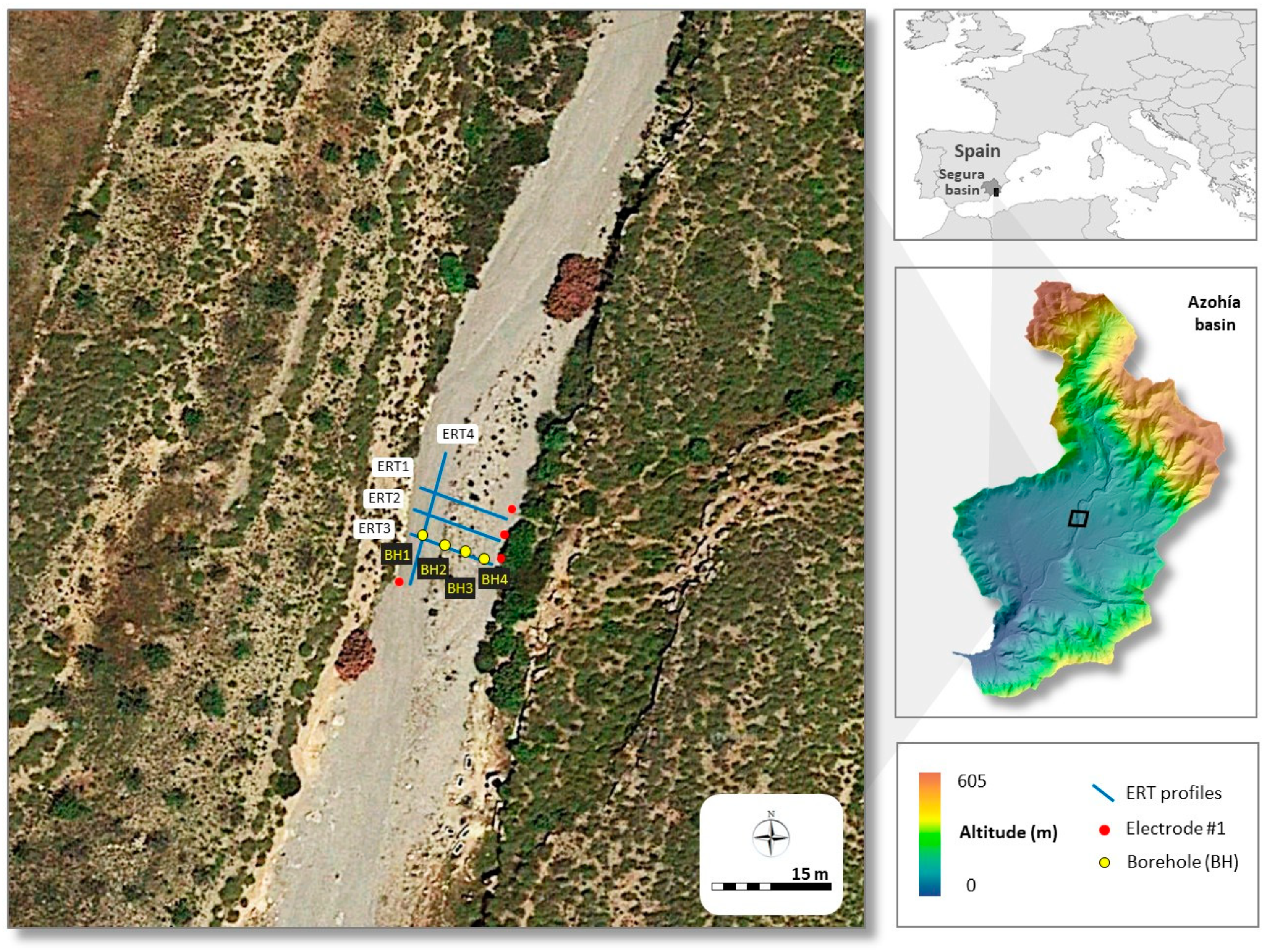
2. Study Area: Geomorphological and Climatic Setting

This study was carried out in an upper stretch of the ephemeral gravel-bed channel known as “Rambla de la Azohía”. The Rambla de la Azohía is located in the Murcia Region, in southeastern Spain (Figure 1). The climate of the study area has strong seasonal contrasts, providing extreme drought patterns with mean annual precipitation values of 300 mm, and ETP values higher than 140 mm per month in the summer season. The rains are very irregular and intense, which can cause large and rapid floods [10]. The land cover shows a low anthropic impact, associated with extensive scrub areas with shrub canopy typically lower than 20% of total vegetation.

Geomorphological activity is particularly active as a consequence of intense weathering of metamorphic materials (e.g., phyllites, schists, and quartzites) on hillslopes and the installation of a dense network of gullies in the headwater areas that supply large amounts of coarse sediments to the ephemeral channels. High rates of bedload transport and significant morphological adjustments are produced by sporadic torrential flows. Consequently, complex bed-forms and sedimentary structures have developed, also associated with recent changes in the magnitude and frequency of hydrological events.

Often, these bed-forms are composed on poorly sorted sediments with mixed grain sizes (sand, gravel, and pebbles). Deposits of different textures alternate in depth with a general tendency to increase in grain size from the bottom up [11]. This alluvial fill rests mainly on a Miocene marl substrate, the fine texture of which contrasts with that of the overlying coarse detrital materials.

3. Materials and Methods

3.1. Electrical Resistivity Tomography (ERT)

Electrical resistivity tomography method is a non-invasive technique. This method is based on a combination of electrical vertical sounding and profiling techniques for gathering subsurface information. ERT uses a basis of four electrodes for acquiring apparent resistivity values in the field. Electrical currents injected into the subsurface employ two electrodes, named current electrodes, which are commonly labelled as A and B. Simultaneously, potential measurements are addressed using another pair of electrodes, named potential electrodes, which are labelled as M and N [12,13]. The four-electrode-based measurement unit principle applies all along the electrical profile, resulting in an over-lapping of layers, allowing for the generation of 2D electrical sections. For 3D models, parallel profiles were conducted, enabling the creation of 3D-format files, which were processed through a next stage by means of an inversion algorithm [14,22].

By using the ERT method, the collection of information from the subsurface will depend on several parameters that are affected by the electrical contrast that defines the subsurface materials. One of these parameters is the investigation depth, where the length of the profile will have a considerable influence on the investigation depth since the more distance is covered by the profile, the deeper the obtained data is [15]. Another key parameter is the type of measurement array, which determines how the measurements will be conducted. Among the different available arrays, this study employed a dipole-dipole array, which offers higher resolution and more detailed imaging. A dipole-dipole array allows for gathering a wider range of measuring points with the same quantity of electrodes [23].

The field data acquisition was conducted with a SuperSting resistivimeter from AGI (Austin, TX, USA) and a gasoline-based power generator from Honda (Valencia, Spain) as a continuous and suitable power supply. The SuperStingTM Wi-Fi R4/IP multielectrode resistivimeter from AGI (Austin, TX, USA) is equipped with 4 channels and 56 stainless steel electrodes, a 56 switch box and measurement resolution for max. 30 nV, which vary according to the voltage level [24].

Figure 1 shows the situation of the ERT profiles and their distributions and covered area. In this case study, a total of four electrical tomography profiles were conducted, where three of which were laid out parallel with a separation of 1.5 m. Those profiles are referred to as ERT1, ERT2, and ERT3, respectively. On the other hand, the ERT profile, named as ERT4, was laid out perpendicular to the others.

ERT4 profile used 56 stainless steel electrodes with a spacing of 0.55 m and a length of 30.25 m. ERT1, ERT2, and ERT3 profiles used 28 stainless steel electrodes with a spacing of 0.55 m and a length of 14.85 m. The investigation depth was ≈6 and 3 m, respectively. Additionally, each electrode was suitably georeferenced using a Leica Zeno 20 GPS equipment (accuracy of ±1 cm) from Leica (Barcelona, Spain).

Before the inversion process, the whole dataset was submitted to pre-processing, consisting of a filtering stage for removing anomalous values and static correction, normalising the variations in resistivity due to the difference in height between electrodes. Then, the terrain topography was incorporated, since any change in the morphology of the terrain affects ERT measurements considerably; and here, the subsequent data inversion was processed [15]. Finally, the dataset was inverted with AGIUSA’s EarthImager2D y 3D software (ver. 2.4.4, 1.5.5) which uses the least squares approach [25].

Not only does the software use the finite-element method to solve the inversion, but it also considers the terrain topography. The inversion process computes a model that fits with the observed data. The inversion computes a theoretical initial model which is compared with the measured data. This initial model is progressively modified for reducing discrepancies between the model response and the measured data. The mean absolute misfit error value quantifies the number of differences between models. The iterative process finishes when the computed and measured data achieve an acceptable convergence value. By using L2-norm (smooth), an accurate model of the subsurface of the channel was generated which fitted coherently with the data acquired from the boreholes [22,26].

Soil moisture values, a determining factor for electrical resistivity tests, should be low to minimize artificial variation in resistivity records. To carry out the tomography (prepared on the 3rd of October 2020), the absence of significant rainfall at least one month before the field campaign was considered. In addition, the reference evapotranspiration (ETo) values shown by the nearest meteorological stations provided high values close to 100 mm in September, which, when combined with the high drainage capacity of the sediments of the riverbed, ensured a low humidity of the soil for proper data collection [27].

3.2. Sediment Texture Analysis from Datasets of Borehole Samples

Stratigraphic alluvial units were sampled from four boreholes of 3 m depth in the upper channel reach of the Rambla de la Azohía. The drilling sites selected correspond to representative bed forms along this stream stretch: two boreholes were located in a longitudinal alluvial bar and another two in lateral channels (main and secondary). Samples were collected from each sedimentary structure for grain size analysis and the calculation of particle shape (Figure 2).

Most of these sediments are unconsolidated materials, whose porosity is closely related to the types of packing, grain shape, arrangement, and particle-size distribution [28]. Finer particles have a more significant effect on porosity than coarse particles [29]. For spherical particles of uniform sizes, the porosity is 47.6% by cubical packing, and 26.0% by rhombohedral packing, which is the most compact packing type [28]. The porosity falls between these two values for other packing classes. However, for porous media in clastic deposits consisting of particles of non-uniform sizes, as in our case, porosity cannot be calculated directly, and other physical properties must be taken into account in addition to the packing effect, such as grain shape, particle size, sorting, and roundness [30]. The primary porosity usually increases as the grain size increases, the sediment is better sorted and more loosely packed, the grains become better rounded, and the clay content decreases [31]. For example, poorly sorted grains generally have closer packing and lower porosity across a wide range of grain sizes, as fine grains tend to fill the void space between large grains. Well-rounded grains with high sphericity should pack with a minimum of pore space [32]. Jin et al. [30] considered four classes of grain packs from different aspect ratios (L/I = 1.0, 1.5, 2.0, 2.5), L/I being defined as the ratio of the length of the longest axis of a grain (L) to that of its shortest axis (I). Its results showed that the spherical grain pack exhibits a higher porosity compared to ellipsoidal grain packs. This effect is also shown in average permeability calculations, where the spherical grain pack exhibits lower permeability. Some typical porosity values of natural sedimentary materials are shown in

Table 1. Typical porosity values of natural sedimentary materials [28].

Sedimentary Materials	Porosity (%)	Sedimentary Materials	Porosity (%)
peat soil	60–80	fine-to-medium mixed sand	30–35
soils	50–60	gravel	30–40
clay	45–55	gravel and sand	30–35
silt	40–50	sandstone	10–20
medium-to-coarse mixed sand	35–40	shale	1–10
uniform sand	30–40	limestone	1–10

.

The median grain size (D₅₀) and 84th percentile (D₈₄) were calculated for each sample. As effective grain sizes were used the 10th (D₁₀) and 20th (D₂₀) percentiles, that is to say, the particle diameter (mm) of 10 and 20% of all sediment is the smallest, respectively by weight. Many authors [33,34,35,36] have already regularly used these diameters to calculate hydraulic conductivity (HC) in detritical deposits. The application D₁₀ as an effective grain size in this case has been limited to uniform sands [37]. However, in the case of gravels and pebbles, we have found a greater relationship between D₂₀ and the ERT results, which can probably be maintained with the HC values. A sorting index (σ) was also adopted as a measure of granulometric dispersion, which takes the expression σ = (D₈₄/D₁₆)^0.5.

The derived metrics, particle-shape indices, maximum projection sphericity index (MPSI), and characterisation of sediment textures lead to improved bedload estimates with reduced uncertainty, as well as improved understanding of the relationships between sediment texture, grain size distribution, and electrical resistivity. To calculate the particle-shape, the Zingg (1935) and the Sneed and Folk (1958) methods were used in this study. Both methods are based on the combination of three orthogonal axial lengths: L, I, and S (respectively, the lengths of the longest, intermediate, and shortest axes of individual clasts), so that L ≥ I ≥ S. The Zingg (1935) method allows for differentiating four classes of shapes (spheroids, blades, discoids, and rods) through a Cartesian coordinate system using the indices S/I and I/L. The ratio S/I discriminates blades and discs (low values) from rods and spheres (high values), while the ratio I/L separates blades and rods (low values) from discs and spheres (high values).

To exhibit shape-sorting properties, the disc:rod index from Sneed and Folk (DRI = (L − I)/(L − S)) was applied. These authors separated oblate (discoid) shapes from prolate (blade and rod) shapes and suggested the combination of DRI with the ratio S/L to produce three end members of shape (disc, rod, and sphere) in a triangular diagram. In addition, we used the effective settling sphericity index of Sneed and Folk (1958) as the maximum projection sphericity of a particle (ψ_p), which is given by the equation ψ_p = (S²/L·I)^1/3.

Void ratios were estimated from the grain size distribution, sphericity and roundness indices, and slenderness ratio [38]. These relationships have already been proven by various authors [39,40]. A wider grain size distribution allows the particles to compact more densely, as the smaller particles fill in the gaps between their larger neighbors. Particles that are more angular pack less tightly, as sharp corners pull them apart. Increasing the slenderness of the particles can decrease the density as the thin particles close the gaps between the grains and create large open voids. To calculate hydraulic conductivity (HK) (m.s⁻¹) we used the Kozeny-Carman equation from effective porosity and characteristic grain sizes, according to its most simplified form [35].

3.3. Statistical Relationship between Texture Parameters and Electrical Resistivity

The Past program was used for the statistical analysis [41]. Shapiro-Wilk W was applied for testing normal distribution. Univariate analysis included examining Pearson’s correlation between sediment texture from borehole logs and the values of resistivity from ETR. The resistivity values correspond to the average of ETR records for each depth section with a homogeneous structure and materials extracted from the boreholes. The tests took two levels of significance for the p value (p < 0.05 ** and p < 0.1 *).

The variables with the highest correlation were selected to develop linear regression models using the least squares method. The values of the texture analysis as dependent variables and the resistivity data as explanatory variables were applied. To further explore the relationship between these variables, the results were adjusted to polynomial models, which served to minimise the variance of the unbiased estimators of the coefficients.

4. Results and Discussion

4.1. Changes in Sediment Texture from Borehole Sample Datasets

Table 2. Representative grain sizes and sorting estimated for clastic sediments in borehole logs. Rambla de la Azohía.

				Grain Sizes
	Depth (m)	D10 (mm)	D20 (mm)	D50 (mm)	D84 (mm)	σ
BH1	0.0–1.1	0.4	2.1	15	36	2.37
	1.1–3.0	0.01	0.02	0.04	0.06	0.08
BH2	0.0–1.4	0.4	2.5	12	27	2.09
	1.4–2.3	0.2	1.1	1.9	15	2.21
	2.3–3.0	0.5	2.6	17	32	2.22
BH3	0.0–1.2	0.4	3.3	10	17	1.86
	1.2–1.6	0.3	1.9	8	18	2.08
	1.6–2.5	0.4	1.4	6	26	2.20
	2.5–3.0	0.1	0.5	4	12	2.73
BH4	0.0–1.5	0.5	3.2	17	27	2.11

BH is the borehole code, D₁₀ and D₂₀ are the effective grain sizes corresponding to 10% and 20% of the total sample weight (mm), D₅₀ is the median grain size (mm), D₈₄ is the particle size for 84% of the sample weight (mm), and σ is the inclusive graphic standard deviation (sorting) after Folk (1974).

shows the characteristic particle sizes and sorting indices obtained for all clastic sediment samples that were extracted from the boreholes. According to these data, different patterns in thickness and sediment texture were found in the alluvial channel-fill: the pattern located in the active channel, characterised by a progressive decrease in the median grain size, and an increase in the sorting index with depth, passing from medium-sized gravels at the surface level to sands and small gravels at the bottom (BH3); the pattern defined in the lateral bars (BH1 and BH4) by a single layer 1 to 1.5 m thick composed of medium and coarse gravels and moderate heterometry (2.1 < σ < 2.4), directly lying on a softer rocky substrate; and a third pattern in the edge and tail part of a central bar (BH2), where a subsurface level of coarse material is prevalent, mainly gravels with a size dispersion index somewhat smaller than in the previous cases, but noting an abrupt change in texture in depth (a layer with abundant sand 1 m thick and a deeper and slightly thinner mixed layer of sands, gravels, and pebbles). In general, except in the BH2 case, the subsurface detritical layer has a homogeneous thickness, between 1 and 1.5 m, and consists of coarser materials than deep deposits.

Average values of the Zingg and the Sneed and Folk shape and sphericity indices for each depth interval are shown in

Table 3. Average values of the Zingg and the Sneed and Folk shape and sphericity indices, estimated for gravels and pebbles in borehole logs. Rambla de la Azohía.

		Zingg Shape Classes												Shape—Sphericity (Sneed & Folk, 1958)
	Depth (m)	Discoid or Oblate			Equid.—Spheroid			Blade			Rod
		%	I/L	S/L	%	I/L	S/L	%	I/L	S/L	%	I/L	S/L	S/L	DRI	ψp
BH1	0.0–1.1	57.1	0.81	0.55	0.0	-	-	14.3	0.45	0.60	28.6	0.58	0.75	0.42	0.51	0.63
	1.1–3.0	Loamy substrate
BH2	0.0–1.4	50.0	0.82	0.50	16.7	0.80	0.71	0.0	-	-	33.3	0.47	0.71	0.41	0.49	0.62
	1.4–2.3	50.0	0.72	0.50	16.7	0.70	0.89	16.7	0.60	0.50	16.7	0.63	0.68	0.40	0.55	0.62
	2.3–3.0	50.0	0.80	0.54	0.0	-	-	50.0	0.61	0.59	0.0	-	-	0.39	0.47	0.60
BH3	0.0–1.2	33.3	0.93	0.46	0.0	-	-	16.7	0.59	0.58	50.0	0.59	0.74	0.42	0.51	0.63
	1.2–1.6	50.0	0.89	0.54	50.0	0.76	0.72	0.0	-	-	0.0	-	-	0.51	0.38	0.69
	1.6–2.5	100.0	0.77	0.60	0.0	-	-	0.0	-	-	0.0	-	-	0.46	0.42	0.65
	2.5–3.0	50.0	0.73	0.49	33.3	0.74	0.75	0.0	-	-	16.7	0.62	0.81	0.44	0.54	0.65
BH4	0.0–1.5	57.1	0.76	0.60	14.3	0.83	0.84	28.6	0.63	0.55	0.0	-	-	0.45	0.49	0.65

S, I and L are measurements of the short, intermediate, and long orthogonal axes of clasts, made from selected sieve intervals that represent the spread in the size distribution of the natural gravel and pebbles; DRI is the disc–rod index (L − I)/(L − S); ψ_p is the effective settling sphericity.

. A common feature in all borehole logs is the decrease in the percentage of rod particles as depth increases. This fact may have conditioned the void ratio and the effective porosity in a similar proportion, also affecting the obtained electrical resistivity values. It is also worth noting the progressive decrease in the I/L ratio in the discoid or oblate class obtained according to the depth for the BH3 borehole. The highest percentages reached in the subsurface layer correspond to the discoid/oblate and rod classes (>80% between both classes), which tend to increase the degree of porosity at this level. On the other hand, the disc-rod index (DRI) and the effective settling sphericity (ψ_p) do not seem to be decisive for differentiating sediment textures, since they range between 0.38 and 0.51 in the first case and between 0.60 and 0.69 in the second.

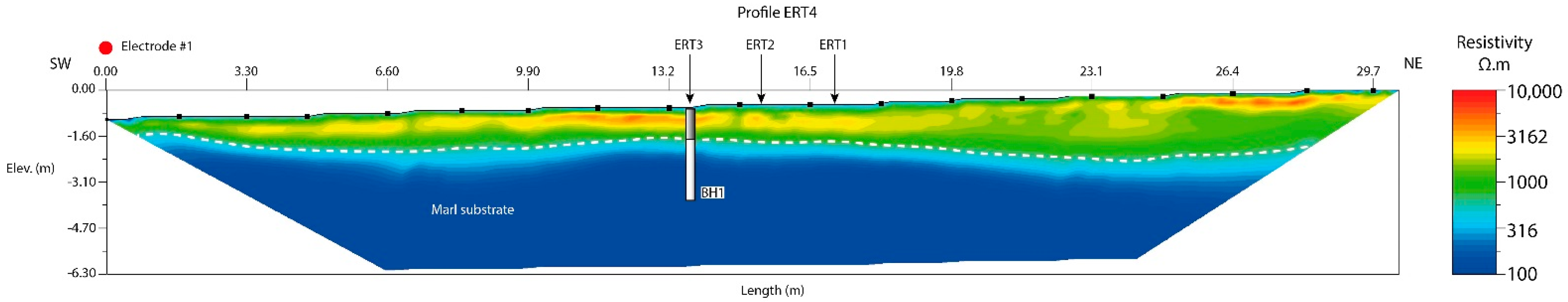
4.2. Electrical Resistivity Tomography 2D Survey

As a general rule, the penetration depth is approximately 15–25% of the longest array length for any four-electrode array [42]. Resistivity results of this study present higher values owing to the sort and material type as Grygar et al. [43] and Chaudhuri et al. [44] have alluded in their study. The ERT4 profile is the largest profile of the whole study that reaches around 6 m of investigation depth. This profile identifies the internal structure of the gravel-bed channel. BH4 was made as to coincide with the ERT4 profile approximately in the central part of the profile, as expected [6,7]. The depth at which the marl substrate is encountered is 1.1 m. Additionally, profile ERT4 intersects with profiles ERT1, ERT2, and ERT3 at 11 m, maintaining a uniform distribution of the position of the marl substrate (Figure 3).

At the top, an alluvial channel-fill is identified with high values of resistivity above ≈600 Ω.m, while at the bottom, the resistivity progressively decreases to low values (<300 Ω.m), indicating the presence of the marl substrate. The white dashed line marks the border between them, see Figure 3.

The ERT4 profile provides a general overview of the channel. The profiles ERT1-ERT3 were limited by the channel width, reaching a depth of investigation of only ≈3 m. Figure 4 shows the resulting 2D geoelectrical sections of ERT1, ERT2, and ERT3 profiles. After the eighth iteration, the ERT1 profile yielded a section with a root mean square (RMS) of 9.47% and 1.05 of L2. In the case of the ERT2 profile, the RMS is 9.51% and L2 = 1.03, and finally, the ERT3 profile presents RMS = 10.21% and L2 = 1.09.

Besides, the profiles ERT1–ERT3 identified the marl substrate featured with lower resistivity values (blue-cyan in the colour bar), which confirms the results obtained from the ERT4 profile. The 2D ERT study reproduced the physical structure of the channel, it presented a central bar and two lateral channels. ERT1 was in the upstream while ERT3 was in the downstream direction. This distribution allowed us to identify the bar geometry, which is wider in ERT1 but narrower in ERT3. The bar presents a triangular form, indicating that the bar decreases in the downstream direction. Four mechanical boreholes were drilled on ERT3 (Figure 4).

Figure 4 presents a horizontal layer with a relatively constant thickness of about ≈1 m which is associated with a high resistivity (>2000 Ω.m). The results from boreholes support ERT results and link this layer to the pattern located in the active channel composed of medium and coarse gravels. The third pattern is related to BH2. In this pattern exists a top layer composed of coarser materials (gravel), corresponding to resistivities > 5000 Ω.m (ERT3) and a second layer of sand layer 1 m thick. The sand layer does not appear in the profile ERT 3 although it appears in profile ERT2 with resistivities > 3000 Ω.m. It was not possible to gather a sample from the material featured in ERT with a green colour (1000–2000 Ω.m); therefore, we cannot define the exact material type (Figure 4).

The results of the 2D study fit coherently with the texture datasets provided by the borehole logs and what is expected for the study area. In general, at the top, a detrital layer, 1.2 m thick, showed especially high ERT values. However, this did not always match the coarser grain sizes. BH3 resistivities between 4000 and 9000 Ω.m were recorded in medium gravels with a significant effective grain size (D₂₀) (3.3 mm), due to matrix composed of clay and sand, which decreased the porosity estimates (ϕ = 0.27) and hydraulic conductivity (CH ≤ 6 10⁻⁴ m.s⁻¹). This high relationship between ERT and D₂₀ was also found in BH2 and BH4, where the highest resistivity (5000 to 8000 Ω.m) occurred in the subsurface deposits with greater D₂₀ grain sizes (2.5 to 3.2 mm), and lower HC (<7 × 10⁻⁴ m.s⁻¹). In BH1, located on the right part of the channel, the upper sedimentary layer (1 m thick) showed moderate ERT values, associated with the presence of medium gravels and higher porosity (ϕ = 0.35). The central part a longitudinal bar has been developed, whose recent evolution reflects a sedimentary pattern typical of several ephemeral gravel-bed streams, which are subjected to the effects of climate change: a progressive decrease in particle size with depth and strong surface armouring. Conversely, the sorting index increased towards the deeper alluvial layers.

4.3. Electrical Resistivity Tomography 3D Modelling

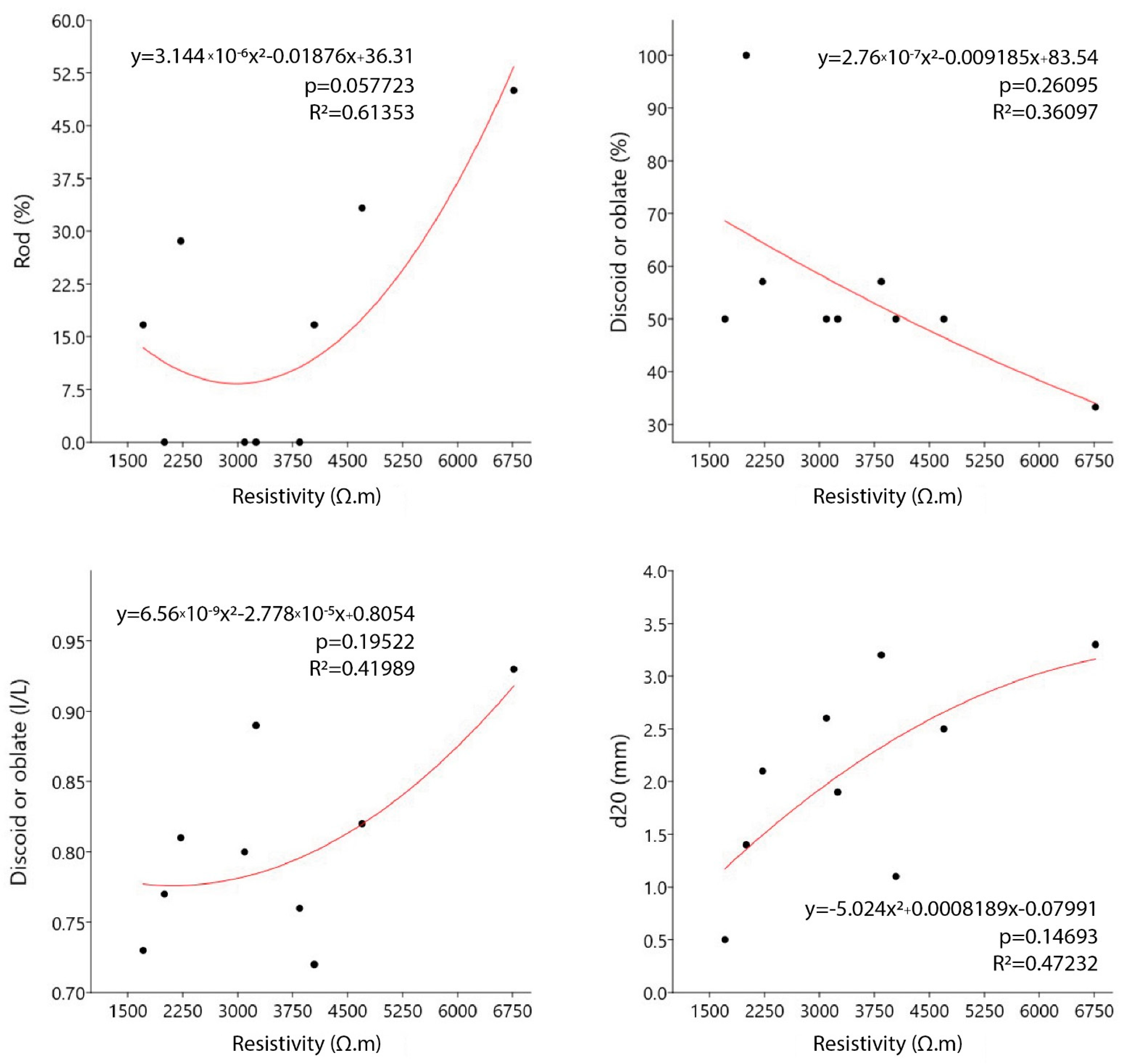
4.3.1. Statistical Relationships

Some significant relationships between physical properties and electrical resistivity tomography were found.

Table 4. Pearson’s correlation results.

	Grain Sizes					Zingg Shape Classes
	D10 (mm)	D20 (mm)	D50 (mm)	D84 (mm)	σ	Discoid or Oblate			Equidimensional—Spheroid			Blade			Rod
						%	l/L	S/L	%	l/L	S/L	%	l/L	S/L	%	l/L	S/L
p	0.48	0.05	0.31	0.52	0.43	0.09	0.09	0.14	0.64	0.11	0.96	0.69	0.66	0.88	0.07	0.66	0.38
r	0.27	0.67	0.36	0.23	0.28	−0.60	0.60	−0.53	−0.18	−0.79	−0.03	0.15	0.27	−0.09	0.63	−0.27	−0.51
n	9	9	10	10	10	9	9	9	9	5	5	9	5	5	9	5	5

p: p value; r: Pearson’s coefficient correlation; n: sample size.

summarises the results. Four variables showed the most significant correlation coefficients. One describes the grain size and the others are linked to the particle shape. Among all, the most significant is D₂₀ with r = 0.67.

Following these correlations, we perform a regression analysis. Figure 5 shows the four regression models obtained. Rod (%), Discoid (I/L), and D₂₀ (mm) present a direct relationship with the resistivity. While one variable increases, the other variable has the same behaviour. Discoid (%) presents an indirect relationship with resistivity, which means that while the resistivity rises, the discoid variable reduces.

4.3.2. 3D Model

As direct measures for supporting the electrical resistivity tomography study, four boreholes were drilled on the ERT3 profile. These were distributed uniformly along the profile.

Table 5. Resistivity results from the ERT study.

		Resistivity Values in Ω.m
	Depth	Max	Min	Mean	SD	COV
	m					%
BH1	0.0–1.1	2543.4	1590.3	2187.2	252.9	11.6
	1.1–3.0	1427.3	318.7	595.9	253.6	42.6
BH2	0.0–1.4	6923.6	3370.8	4695.5	1303.5	27.8
	1.4–2.3	4304.8	3558.7	4023.4	211.6	5.3
	2.3–3.0	3558.7	2919.3	3160.4	228.4	7.2
BH3	0.0–1.2	8599.2	3744.0	6623.5	1447.4	21.9
	1.2–1.6	3744.0	2694.3	3180.3	309.8	9.7
	1.6–2.5	2694.3	1716.1	1984.3	276.4	13.9
	2.5–3.0	1716.1	1706.3	1710.0	4.3	0.3
BH4	0.0–1.5	7183.5	1832.7	3843.7	1665.2	43.3

BH: Boreholes, SD: Standard deviation, COV: Coefficient of variation.

contains the summary of the study results. Samples at different depths of each borehole were employed to perform the analysis. A 3D model is a proven tool that contributes significantly to identifying different subsurface structures used in several studies [45,46].

The 3D model computed with the electrical resistivity tomography data identified the same changes in sediment texture (patterns) as those found in the grain size study [47]. The colour bar of the model was calibrated with 1000 Ω.m as the step value. This value allowed for the distinguishing of the underground formations previously found in the 2D study, and the visualising of the extent of them simultaneously. Figure 6 shows the different patterns, which varied in accordance with the increase/decrease in the resistivity.

Figure 6 shows the 3D model; this model has four vertical sections in the same place where the boreholes were drilled, aiming to facilitate the data interpreting process and visualising how the material evolves in that space. Figure 6a–f presents the different layers and body formations continuously. Notice that while the resistivity values rise, materials tend to group in the central site of the model, which corresponds to bar place.

Figure 6a represents to the lowest resistivity values (0–1000 Ω.m) of the whole study. These values belong to the softer rocky substrate, which is in line with BH1 results, and show that the model is a realistic reproduction of the study area. Figure 6b presents a new layer featured with the green colour (1000–2000 Ω.m), which is spread in the whole model. This layer, representing medium gravel with little clay matrix, cut the borehole BH4 at 1.5 m deep. Since the samples collected from BH4 only reached to a depth of 1.5 m, this pattern was not contemplated in the granulometric study; however, the ERT detected its presence.

Figure 6c–f, with values of resistivity >2000 Ω.m, represent the layer 1 to 1.5 m thick, which is common in all boreholes, except in BH2, composed mainly of medium and coarse gravels. The layer disposition in the 3D model adopts an onion-like shape, finding the least resistivity values in the external part and the most resistant in the core. Values of resistivity ranging from 2000 to 3000 Ω.m (Figure 6c) are linked to the green-yellow colour, forming a layer in the model that constrains in the lateral direction of the bar by 6–8 m, acquiring a shell form at the bottom of the model.

The inner part of the onion-like structure is represented in Figure 6d–f, which is focused on BH2 (7.5 m). The upper part of the borehole (Figure 6f) corresponds to coarse materials (gravel and pebbles) linked to resistivity values above 5000 Ω.m. An intermediate layer (Figure 6d,e), 1 m thick, composed of gravel with abundant sand, reduces the range of resistivity at the middle stretch of BH2 (3000–5000 Ω.m).

In general, the 3D model detected in the central channel part an upper subsurface layer of 1–1.2 m thick, with resistivities above 4500 Ω.m, which corresponded to the coarsest materials (gravel and pebbles) and gravels with a supported matrix. In addition, resistivity reduces according to depth (Table 5), owing to a progressive decrease in the median grain size and an increase in the sorting index with depth. The lateral parts, close to the banks, have undergone a different geomorphological evolution: the right side currently constitutes the active channel of low waters, with a uniform bed composed of medium gravels, which, during much of the filling period, received finer-sized materials (small gravels and sands). The resistivities in this case decreased from 4000 Ω.m at the top to 500 Ω.m at the limit with the loamy substrate. On the other hand, the left part shows a higher concentration of thicker sediments due to the presence of a lateral bar still under development today, which is in accordance with the measured ERT values in the 3D model (>4500 Ω.m).

5. Conclusions

The physical characterisation of the alluvial deposit was successfully completed. The resistivity trend is high, owing to the presence of air and the loose nature of the materials. The 3D ERT models obtained have allowed for the estimation of both the vertical and horizontal variations of the thickness, and the characterisation of the different materials. Borehole logs are a punctual sample, whereas electrical resistivity tomography allows for inferring the 3D information of the deposit.

The combination of electrical resistivity tomography, 2D and 3D, with some borehole logs have demonstrated that they are a useful methodology for assessing alluvial deposits. Consequently, the ERT results coupled with borehole data suggest that from the channel entrenchment in the Miocene marl substrate, different pulses of vertical sedimentary accretion were produced, denoting a general trend of increasing grain size (coarsening upwards) towards the top of the sedimentary sequence.

References

1. Bull, W.B. Discontinuous ephemeral streams. Geomorphology 1997, 19, 227–276. [Google Scholar] [CrossRef]
2. Segura-Beltrán, F.; Sanchis-Ibor, C. Assessment of channel changes in a Mediterranean ephemeral stream since the early twentieth century. The Rambla de Cervera, eastern Spain. Geomorphology 2013, 201, 199–214. [Google Scholar] [CrossRef]
3. Norman, L.M.; Sankey, J.B.; Dean, D.; Caster, J.; DeLong, S.; DeLong, W.; Pelletier, J.D. Quantifying geomorphic change at ephemeral stream restoration sites using a coupled-model approach. Geomorphology 2017, 283, 1–16. [Google Scholar] [CrossRef]
4. Vásconez-Maza, M.D.; Martínez-Segura, M.A.; Bueso, M.C.; Faz, Á.; García-Nieto, M.C.; Gabarrón, M.; Acosta, J.A. Predicting spatial distribution of heavy metals in an abandoned phosphogypsum pond combining geochemistry, electrical resistivity tomography and statistical methods. J. Hazard. Mater. 2019, 374, 392–400. [Google Scholar] [CrossRef] [PubMed]
5. Martínez-Segura, M.A.; Vásconez-Maza, M.D.; Faz, Á.; Martínez-Martínez, S.; Gabarrón, M.; Acosta, J.A. Assessment of the environmental impact of an agricultural area near a coastal lagoon using geophysical and geochemical techniques. In Recent Advances in Geophysics; Nova Science Publishers, Inc.: Hauppauge, NY, USA, 2019; ISBN 978-1-53616-207-3. [Google Scholar]
6. Uhlemann, S.; Kuras, O.; Richards, L.A.; Naden, E.; Polya, D.A. Electrical resistivity tomography determines the spatial distribution of clay layer thickness and aquifer vulnerability, Kandal Province, Cambodia. J. Asian Earth Sci. 2017, 147, 402–414. [Google Scholar] [CrossRef] [Green Version]
7. Bábek, O.; Sedláček, J.; Novák, A.; Létal, A. Electrical resistivity imaging of anastomosing river subsurface stratigraphy and possible controls of fluvial style change in a graben-like basin, Czech Republic. Geomorphology 2018. [Google Scholar] [CrossRef]
8. Chambers, J.; Ogilvy, R.; Kuras, O.; Cripps, J.; Meldrum, P. 3D electrical imaging of known targets at a controlled environmental test site. Environ. Geol. 2002, 41, 690–704. [Google Scholar] [CrossRef]
9. Ogilvy, R.D.; Meldrum, P.I.; Kuras, O.; Wilkinson, P.B.; Chambers, J.E.; Sen, M.; Pulido-Bosch, A.; Gisbert, J.; Jorreto, S.; Frances, I.; et al. Automated monitoring of coastal aquifers with electrical resistivity tomography. Near Surf. Geophys. 2009, 7, 367–376. [Google Scholar] [CrossRef] [Green Version]
10. Ortega, J.A.; Razola, L.; Garzón, G. Recent human impacts and change in dynamics and morphology of ephemeral rivers. Nat. Hazards Earth Syst. Sci. 2014, 14, 713–730. [Google Scholar] [CrossRef] [Green Version]
11. Conesa-García, C.; Puig-Mengual, C.; Riquelme, A.; Tomás, R.; Martínez-Capel, F.; García-Lorenzo, R.; Pastor, J.L.; Pérez-Cutillas, P.; Cano Gonzalez, M. Combining sfm photogrammetry and terrestrial laser scanning to assess event-scale sediment budgets along a gravel-bed ephemeral stream. Remote Sens. 2020, 12, 3624. [Google Scholar] [CrossRef]
12. Everett, M.E. Near-Surface Applied Geophysics; Cambridge University Press: Cambridge, UK, 2013; ISBN 9781107018778. [Google Scholar]
13. Vásconez-Maza, M.D.; Martínez-Pagán, P.; Aktarakçi, H.; García-Nieto, M.C.; Martínez-Segura, M.A. Enhancing Electrical Contact with a Commercial Polymer for Electrical Resistivity Tomography on Archaeological Sites: A Case Study. Materials 2020, 13, 5012. [Google Scholar] [CrossRef] [PubMed]
14. AGI EarthImager 3D Resistivity Software. Available online: https://www.agiusa.com/agi-earthimager-3d (accessed on 2 February 2021).
15. Loke, M.H. Tutorial:2-D and 3-D Electrical Imaging Surveys. Available online: http://citeseerx.ist.psu.edu/viewdoc/download?doi=10.1.1.454.4831&rep=rep1&type=pdf (accessed on 5 March 2019).
16. Kasprzak, M. High-resolution electrical resistivity tomography applied to patterned ground, Wedel Jarlsberg Land, south-west Spitsbergen. Polar Res. 2015, 34, 1–13. [Google Scholar] [CrossRef] [Green Version]
17. Greggio, N.; Giambastiani, B.M.S.; Balugani, E.; Amaini, C.; Antonellini, M. High-resolution electrical resistivity tomography (ERT) to characterize the spatial extension of freshwater lenses in a salinized coastal aquifer. Water 2018, 10, 1067. [Google Scholar] [CrossRef] [Green Version]
18. Rubio-Melendi, D.; Gonzalez-Quirós, A.; Roberts, D.; García García, M.D.C.; Caunedo Domínguez, A.; Pringle, J.K.; Fernández-Álvarez, J.P. GPR and ERT detection and characterization of a mass burial, Spanish Civil War, Northern Spain. Forensic Sci. Int. 2018, 287, e1–e9. [Google Scholar] [CrossRef] [PubMed]
19. Dépret, T.; Virmoux, C.; Gautier, E.; Piégay, H.; Doncheva, M.; Plaisant, B.; Ghamgui, S.; Mesmin, E.; Saulnier-Copard, S.; de Milleville, L.; et al. Lowland gravel-bed river recovery through former mining reaches, the key role of sand. Geomorphology 2021, 373, 107493. [Google Scholar] [CrossRef]
20. Blackburn, J.; Comte, J.-C.; Foster, G.; Gibbins, C. Hydrogeological controls on the flow regime of an ephemeral temperate stream flowing across an alluvial fan. J. Hydrol. 2021, 595, 125994. [Google Scholar] [CrossRef]
21. Rey, J.; Martínez, J.; Hidalgo, M.C. Investigating fluvial features with electrical resistivity imaging and ground-penetrating radar: The Guadalquivir River terrace (Jaen, Southern Spain). Sediment. Geol. 2013, 295, 27–37. [Google Scholar] [CrossRef]
22. Loke, M.H.; Chambers, J.E.; Rucker, D.F.; Kuras, O.; Wilkinson, P.B. Recent developments in the direct-current geoelectrical imaging method. J. Appl. Geophys. 2013, 135–156. [Google Scholar] [CrossRef]
23. AGI Dipole-Dipole Array. Available online: https://www.agiusa.com/dipole-dipole-array (accessed on 16 July 2020).
24. AGI SuperSting Wi-Fi. Available online: https://www.agiusa.com/supersting-wifi (accessed on 16 July 2020).
25. Loke, M.H.; Barker, R.D. Rapid least-squares inversion of apparent resistivity pseudosections by a quasi-Newton method1. Geophys. Prospect. 1996, 44, 131–152. [Google Scholar] [CrossRef]
26. Chambers, J.E.; Wilkinson, P.B.; Wardrop, D.; Hameed, A.; Hill, I.; Jeffrey, C.; Loke, M.H.; Meldrum, P.I.; Kuras, O.; Cave, M.; et al. Bedrock detection beneath river terrace deposits using three-dimensional electrical resistivity tomography. Geomorphology 2012, 177–178, 17–25. [Google Scholar] [CrossRef] [Green Version]
27. SIAM Ficha de Estaciones. Available online: http://siam.imida.es/apex/f?p=101:1000:6322900036254158::NO::: (accessed on 17 March 2021).
28. Bear, J. Dynamics of Fluids in Porous Media; Dover Publications, Inc.: New York, NY, USA, 2013; ISBN 978-0-486-65675-5. [Google Scholar]
29. Salisbury, J.W.; Eastes, J.W. The effect of particle size and porosity on spectral contrast in the mid-infrared. Icarus 1985, 64, 586–588. [Google Scholar] [CrossRef]
30. Jin, G.; Torres-Verdín, C.; Lan, C. Pore-level study of grain-shape effects on petrophysical properties of porous media. In Proceedings of the SPWLA 50th Annual Logging Symposium 2009, The Woodlands, TX, USA, 21–24 June 2009. [Google Scholar]
31. Tucker, M. Sedimentary Petrology: An Introduction to the Origin of Sedimentary Rocks, 3rd ed.; Blackwell Science Ltd.: Oxford, UK, 2001; ISBN 978-0-632-05735-1. [Google Scholar]
32. Beard, D.C.; Weyl, P.K. Influence of Texture on Porosity and Permeability of Unconsolidated Sand. Am. Assoc. Pet. Geol. Bull. 1973, 57. [Google Scholar] [CrossRef]
33. Vukovic, M.; Soro, A. Determination of Hydraulic Conductivity of Porous Media from Grain-Size Composition; Water Resources Publications: Littleton, CO, USA, 1992; ISBN 9780918334770. [Google Scholar]
34. Cheng, C.; Chen, X. Evaluation of methods for determination of hydraulic properties in an aquifer-aquitard system hydrologically connected to a river. Hydrogeol. J. 2007, 15, 669–678. [Google Scholar] [CrossRef]
35. Odong, J. Evaluation of Empirical Formulae for Determination of Hydraulic Conductivity based on Grain-Size Analysis. J. Am. Sci. 2007, 3, 54–60. [Google Scholar]
36. Koch, K.; Kemna, A.; Irving, J.; Holliger, K. Impact of changes in grain size and pore space on the hydraulic conductivity and spectral induced polarization response of sand. Hydrol. Earth Syst. Sci. 2011, 15, 1785–1794. [Google Scholar] [CrossRef] [Green Version]
37. Urumovi, K.; Urumović, K., Sr. The effective porosity and grain size relations in permeability functions. Hydrol. Earth Syst. Sci. Discuss. 2014, 11, 6675–6714. [Google Scholar] [CrossRef]
38. Cho, G.-C.; Dodds, J.; Santamarina, J.C. Particle Shape Effects on Packing Density, Stiffness, and Strength: Natural and Crushed Sands. J. Geotech. Geoenvironmental Eng. 2006, 132, 591–602. [Google Scholar] [CrossRef] [Green Version]
39. Dodds, J.; Santamarina, C.; Paul Mayne Glenn Rix, A. Particle Shape and Stiffness-Effects on Soil Behavior; Georgia Institute of Technology: Atlanta, GA, USA, 2003. [Google Scholar]
40. Rousé, P.C.; Fannin, R.J.; Shuttle, D.A. Influence of roundness on the void ratio and strength of uniform sand. Géotechnique 2008, 58, 227–231. [Google Scholar] [CrossRef]
41. Hammer, Ø.; Harper, D.A.T.; Ryan, P.D. PAST: Paleontological Statistics Software Package for Education and Data Analysis. Palaeontol. Electron. 2001, 4, 1–9. [Google Scholar]
42. AGI Quick Tip: Depth of Investigation for ERI Surveys. Available online: https://www.agiusa.com/blog/quick-tip-depth-investigation-eri-surveys (accessed on 28 February 2021).
43. Matys Grygar, T.; Elznicová, J.; Tůmová, S.; Faměra, M.; Balogh, M.; Kiss, T. Floodplain architecture of an actively meandering river (the Ploučnice River, the Czech Republic) as revealed by the distribution of pollution and electrical resistivity tomography. Geomorphology 2016. [Google Scholar] [CrossRef]
44. Chaudhuri, A.; Sekhar, M.; Descloitres, M.; Godderis, Y.; Ruiz, L.; Braun, J.J. Constraining complex aquifer geometry with geophysics (2-D ERT and MRS measurements) for stochastic modelling of groundwater flow. J. Appl. Geophys. 2013, 98, 288–297. [Google Scholar] [CrossRef]
45. Zeng, R.Q.; Meng, X.M.; Zhang, F.Y.; Wang, S.Y.; Cui, Z.J.; Zhang, M.S.; Zhang, Y.; Chen, G. Characterizing hydrological processes on loess slopes using electrical resistivity tomography—A case study of the Heifangtai Terrace, Northwest China. J. Hydrol. 2016, 541, 742–753. [Google Scholar] [CrossRef]
46. Argote-Espino, D.L.; López-García, P.A.; Tejero-Andrade, A. 3D-ERT geophysical prospecting for the investigation of two terraces of an archaeological site northeast of Tlaxcala state, Mexico. J. Archaeol. Sci. Rep. 2016, 8, 406–415. [Google Scholar] [CrossRef]
47. Chambers, J.E.; Wilkinson, P.B.; Penn, S.; Meldrum, P.I.; Kuras, O.; Loke, M.H.; Gunn, D.A. River terrace sand and gravel deposit reserve estimation using three-dimensional electrical resistivity tomography for bedrock surface detection. J. Appl. Geophys. 2013, 93, 25–32. [Google Scholar] [CrossRef] [Green Version]
Figure 1. Study area. ERT profiles distribution, red marker determines the beginning of the electrical profile.
Applsci 11 03030 g001
Figure 2. Sediment texture observed on the surface ((a): active channel, (b): transition area between active channel and central alluvial bar, (c): central bar platform) and in the depth of the trench sections ((d): sub-surface layer 1 m deep in the active channel area, (eh): sub-surface layers 1–1.5 m thick from top to bottom in a bar sedimentary sequence), and (i): representative texture of the alluvial fan body cut by the Rambla de la Azohía in its upper reach.
Applsci 11 03030 g002
Figure 3. Perpendicular ERT profile ERT4. The other three profiles intersect vertical with arrows to mark the position of ERT1-ERT3.
Applsci 11 03030 g003
Figure 4. (ac) Parallel ERT profiles (ERT1-ERT3). ERT4 intersects all profiles. BH1-BH4 are the boreholes drilled in the study area. (d). Lithology from BH1-BH4.
Applsci 11 03030 g004
Figure 5. Regression models showing the relationships between resistivity and particle-shape variables.
Applsci 11 03030 g005
Figure 6. 3D model. (af) illustrates the different layers detected by the electrical resistivity tomography survey.
Applsci 11 03030 g006