1. Introduction
In the last twenty years, the interest in exoplanet detection has been increased. More than 4000 planets have been discovered [
1], The main interest of the scientific community are the earthlike planets [
2].
The overwhelming majority of discovering planet was discovered by indirect techniques such as transit light curves [
3], radial velocity [
4], and gravitational microlensing [
5]. These techniques sense the effect of the planet over the star radiation. They measure variations in the star radiation and determine the planet presence using statistical techniques. However, these variations may be produced by unknown processes in the star and not by the presence of a planet. Additionally, the measurements obtained by the microlensing technique are not repeatable because they require the alignment of two stars and the planet. Moreover, the time necessary to perform a measurement employing indirect techniques may last from days to years because the planet must complete at least one orbit.
The direct detection of an exoplanet will confirm the currently available evidence for its existence, with shorter observation periods and incorporating the repeatability ofthe measurement.
The principal challenges in the direct detection of exoplanets are the image resolution and the signal-to-noise ratio. The image resolution refers to the minimum angular distance between two discernible sources. This angular distance is conditioned by the diameter of the primary mirror of the telescope. The signal-to-noise ratio may be defined as the quotient between the planet radiance and the star radiance. At visible wavelengths, the planet radiance arises primarily from the radiation reflected from its parent star. The amount of reflected radiation depends on the planet’s albedo, its radius, and its distance from the star. This ratio for a Jupiter-like planet and a Sun-like star is at least
[
6]. In the infrared (IR) spectral region, the planet radiance consists primarily of the planet thermally emitted radiation. Additionally, the radiance for a Sun-like star is lower in the IR than in the visible region. Under these conditions, the radiation signal-to-noise ratio increases up to
[
7]. However, this is still a very low signal-to-noise ratio. In order to improve the radiation ratio, a coronagraph and interferometric techniques are often implemented [
8,
9].
The coronagraph technique consists of occulting the star using a mechanical aperture. This technique usually implements spatial transmission filters in the focal plane to remove the diffraction rings due to the hard stop edge [
10,
11]. However, due to the limitations of the spatial resolution, this technique is applied primarily to the potential planets with large orbits.
Most of interferometric techniques attenuate the star radiation by means of destructive interference. Consequently, these interferometers are called Nulling Interferometers. They interfere with the wavefronts with a delayed version of them. When the delay between the interferometer arms is
, the star radiation is canceled, with only the planet radiation remaining [
12,
13,
14].
Previously, we proposed a Rotational Shearing Interferometer (RSI) for planet detection [
15,
16,
17,
18]. This interferometer interferes with the wavefronts with a rotated and delayed version of them. Thus, this interferometer may cancel the star radiation in a similar way to the nulling interferometers. Additionally, we may discriminate against false-positive results rotating the wavefront. Unfortunately, when the star is canceled, the remaining amount of radiation is too small. In order to improve the signal magnitude, we propose using the RSI without the total-cancellation of the star radiation. When the star-radiation is not canceled, the fringe visibility is decreased, but the signal magnitude is further increased.
In this work, we describe the response of the RSI to a star–planet system radiation in
Section 2. In
Section 3, we present computational simulations to validate the viability of the method. Finally, we present the conclusions.
2. Theory
The closest star to Earth is Proxima Centauri, its distance to the Earth is 1.295 parsecs [
19]. At this distance, the optical radiation from a massive light source like a star or a planet may be considered coherent. This is because these conditions satisfy the Van Cittert–Zernike theorem [
20]. Then, the radiation from any planetary-system outside the solar system may interfere between them. Additionally, the star and the planet may be considered as point sources [
21].
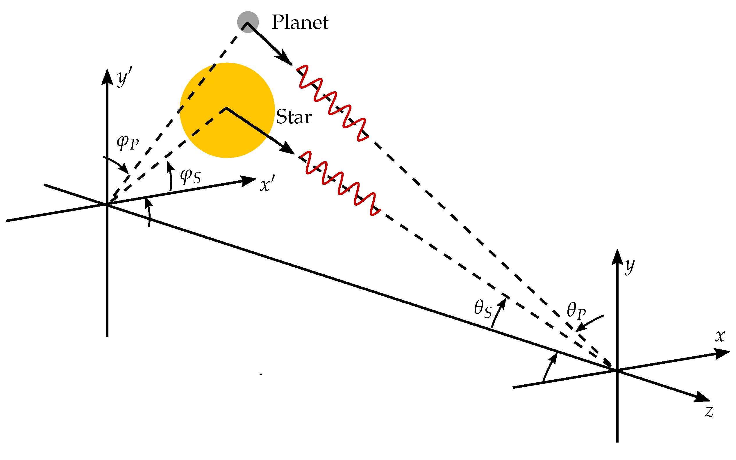
Figure 1 shows a diagram of the star–planet system viewed for the observer. The alignment of the planet and the star is characterized by means of their elevation angle (
) and their azimuth angle (
). The wavefronts from a star or a planet in its periphery may be modeled as planes with uniform intensity due to the long distance from the observer.
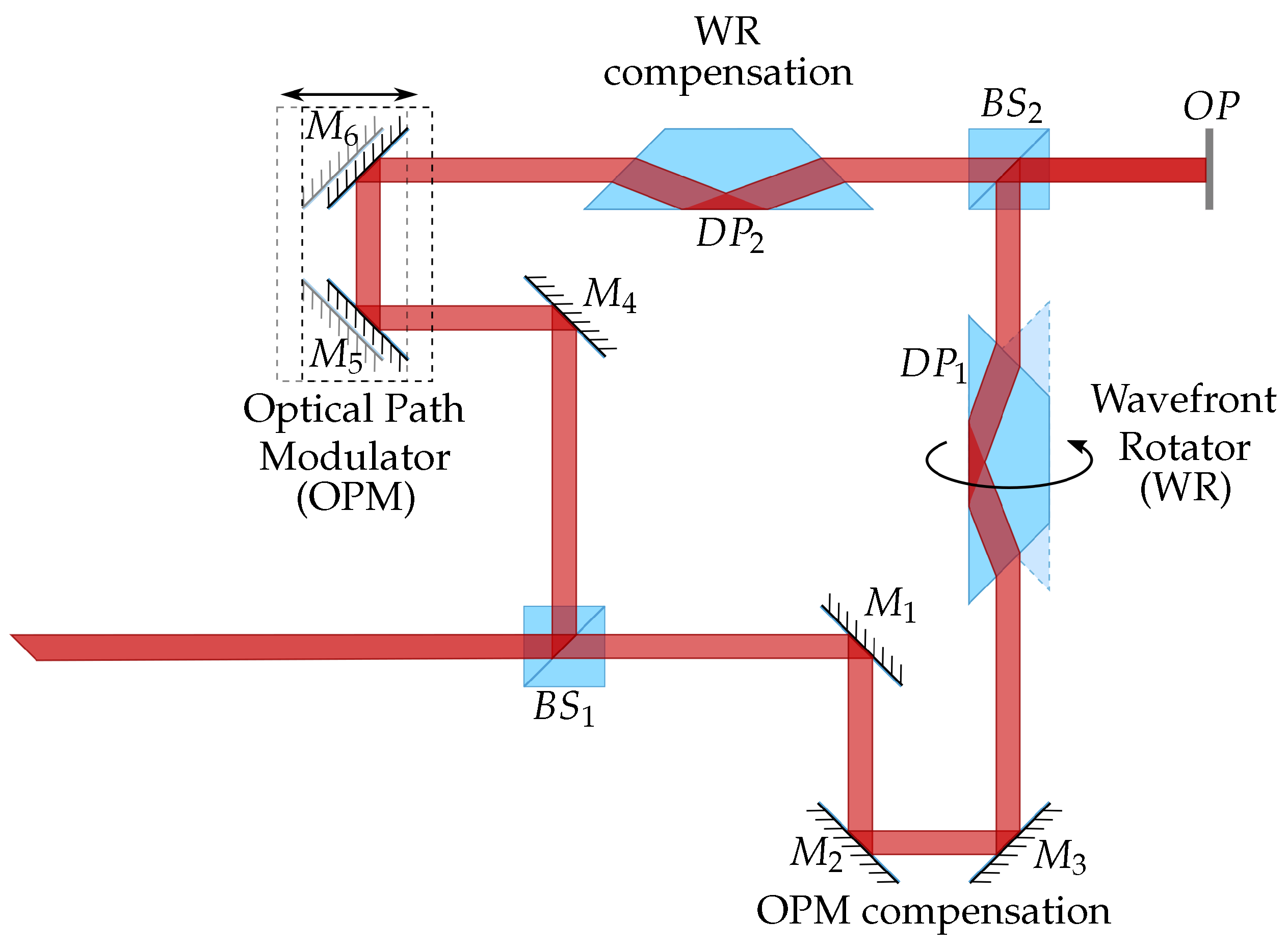
The Rotational Shearing Interferometer (RSI) was proposed for extra-solar planet detection because it is insensitive to rotational-symmetrically wavefronts. The RSI makes incident wavefront interfere with a rotated version of them. When a solitary star is aligned on the optical axis of the interferometer, its wavefront is rotational-symmetrically, and the RSI does not produce a fringe pattern. Instead, when the wavefronts from the star and the planet are incident on the RSI, its interference produces a fringe pattern. The RSI consists of a Mach–Zehnder interferometer with a Dove prism in each arm as shown in
Figure 2. When the Dove prism rotates around the optical axis, the propagated wavefront rotates double of the Dove-prism rotation angle. One of the Dove prism is rotated in order to generate the wavefront rotation. The other Dove prism remains static for compensation purposes. We use a mirror array as an Optical Path Modulator (OPM). This array is formed by the mirrors
,
, and
. The mirrors
and
are collocated over a displacement platform to control the elongation of the optical Path. We add an additional mirror array in the other arm for compensation purposes. When a beam insides on the first beam splitter, it is divided in two. The first one is propagated trough the prism
, and it is rotated by
with respect to the other beam. The second beam is propagated through the OPM to adjust the OPD. Finally, both beams interfere in the observation plane (OP).
When a beam coming from a star–planet system is incident on the RSI entrance, four wavefronts interfere between them on the observation plane. Two of these wavefronts correspond to the planet and the other two correspond to the star. The resulting interference may be divided into three terms: the first one for the interference between the star wavefronts (
), the second one for the interference between the planet wavefronts (
), and an additional term for the interference between the planet and the star wavefronts (
. Then, the incidance (
M) in the interference plane may be modeled as the sum of the terms:
Specifically, these terms may be written in terms of the incidance of the star (
), incidance of the planet (
) and phase (
) of each wavefront. The subscripts
and
, represent the wavefronts, and the interferometer arms, respectively:
Furthermore, the phase term (
) in cylindrical coordinates for each wavefront is modeled by:
We use to denote the optical path length of each interferometer arm. The terms and are used to indicate the elevation and the azimuthal angles between the star and the optical axis, respectively. In similar way, and are the angles between the planet and the optical axis.
2.1. Special Cases
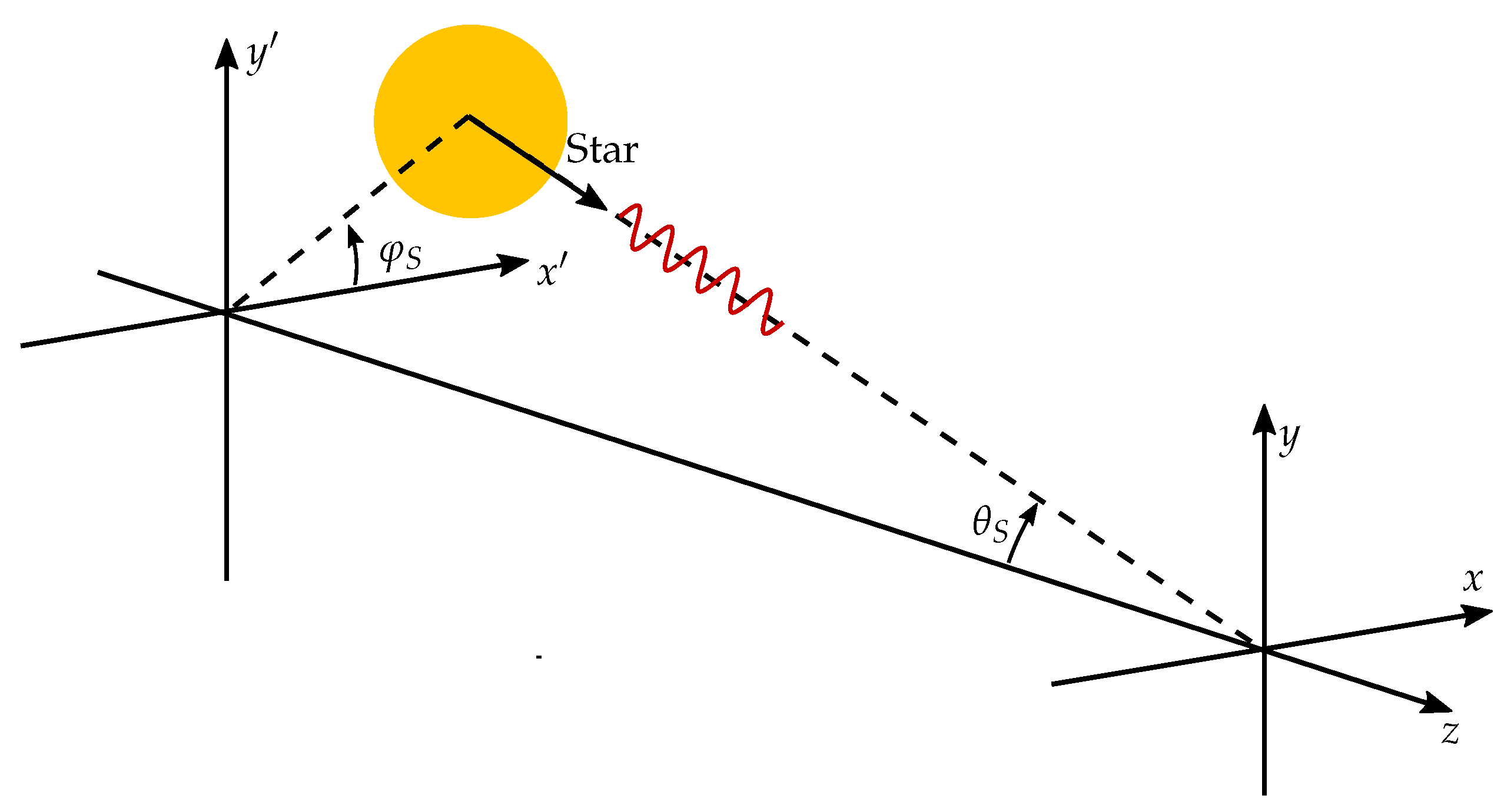
In order to simplify the analysis of these equations, we consider three special cases. In the first case, the star does not have a planet around it (
), and the optical-path-difference (OPD) of the interferometer (
) is equal to
. This case is illustrated in
Figure 3. The second case occurs when the optical axis aligned on the star (
) and the OPD is
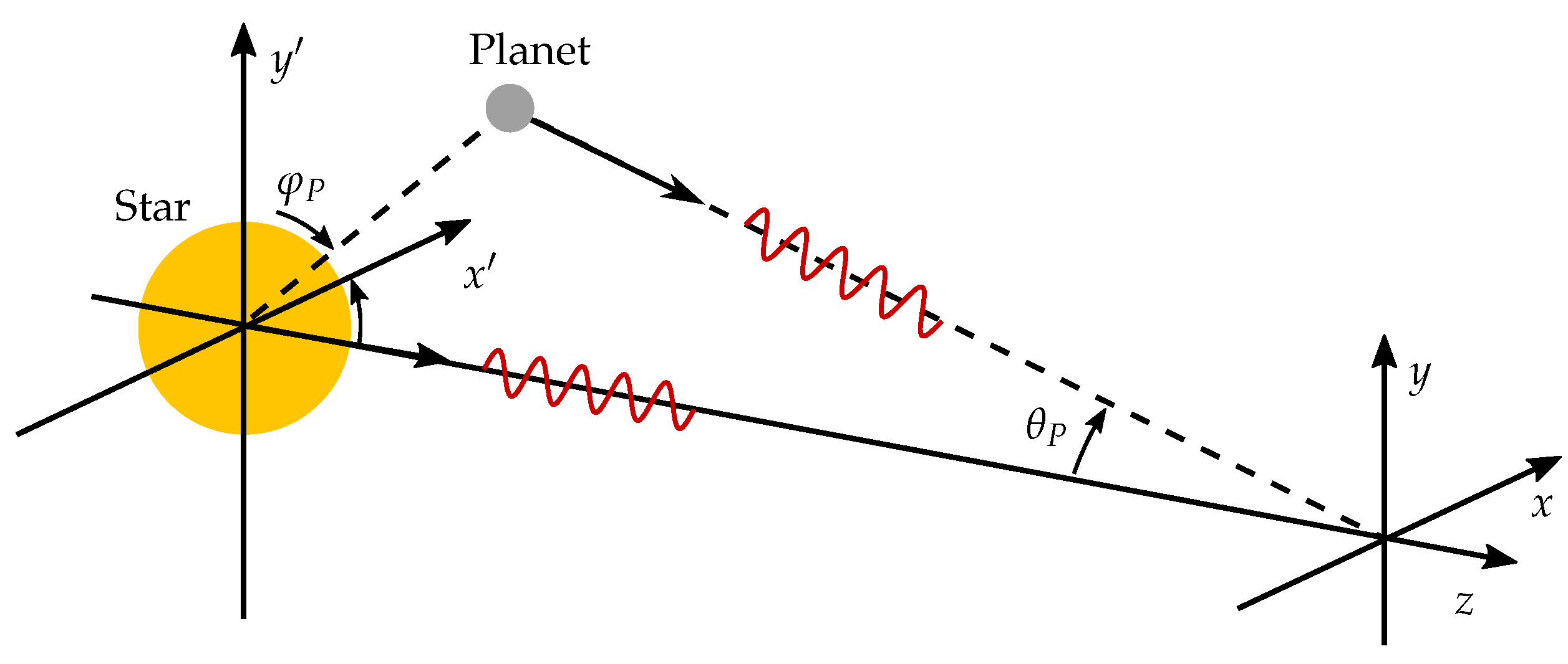
; in this case, the star wavefronts are canceled. Finally, we consider the case when the star is perfectly aligned with the star, but the OPD is different to
(the star wavefront is not canceled).
Figure 4 illustrates the star and planet alignment for the second case and the third case.
2.1.1. First Case, the Solitary Star
When the star does not have a planet as a companion, the interference equation is reduced to the term
, described by the next equation:
Equation (
6) represents a fringe pattern. The spatial frequency of the fringes is given by
. This equation denotes the dependency of the fringe density with the elevation angle of the star. The orientation of the fringe-pattern is given by
. Note that the azimuth angle of the star determines the fringe direction. Because of the dependence between the fringe pattern and the star alignment, we may use this fringe pattern to align the optical axis with the star. When the star is perfectly aligned with the optical axis, the resultant pattern consists of a uniform incidance over the entire observation plane. If we change the interferometer OPD, the incidance level varies accordingly with:
If we adjust the OPD to , the star incidance is canceled at the observation plane. Under these conditions, it is possible to detect a planet if it is present around the planet.
2.1.2. Second Case, Star on Axis and OPD Equal to
When the star is aligned with the optical axis and it is orbited by a planet, the RSI receives the star and the planet wavefronts simultaneously. If additionally, we adjust the OPD to
, the star wavefront is canceled by destructive interference. This case is analyzed in the most of interferometric methods to detect extra-solar planets. The incidance equation is considerably reduced because the terms
and
are canceled; additionally,
is small enough to use the paraxial approximation. The resulting equation may be rewritten as:
Equation (
8) represents a fringe pattern with spatial frequency equal to
and orientation equal to
. Both expressions are dependent on the rotation angle,
. This demonstrates that the frequency and orientation on the fringes may be controlled by the operator as it is shown in laboratory implementations [
22]. The maximum fringe density is reached when the angle between the Dove prisms is
. The minimum fringe separation is
(about 2 m for a Jupiter-like planet at 10 parsecs from the Earth, observed at 10
m).
In this case, the fringe visibility is only limited by the coherence function of the incident beam. Unfortunately, the incidance is too low because the planet incidance
is just a few photons/s per m
[
15].
2.1.3. Third Case, Star on Axis and OPD ≠
In order to increase the signal incidance, we propose using the RSI without a total star cancellation. In these conditions, the fringe visibility is reduced, but the signal amplitude is enhanced considerably. If we consider the star on axis (
) and ignore some phase terms, we may simplify Equations (
2)–(
4) to the next equations:
Note that Equation (
9) is equal to Equations (
7) and (
10) is equal to Equation (
8). Accordingly, these terms produce a background incidance and a fringe pattern. Furthermore, the interference between the planet and the star, represented by Equation (
11), produces two superposed fringe patterns. The first one oriented to
and the second one oriented to
. Their magnitude is modulated by the cosine of
. Their spatial frequency is
, and their fringe separation is
(about 4 m for a Jupiter-like planet at 10 parsecs from the Earth, observed at 10
m). The fringe visibility is reduced for the background incidance, which is increased; accordingly, the OPD moves away
. However, the amplitude of the fringe patterns generated by
is increased too. The decrease of the fringe visibility could persuade the researcher of this way. Notwithstanding, however as long as the detector is not saturated, the signal may be retrieved by image processing. In this way, we may amplify the signal several times until the detector saturates. The maximum signal amplification depends on the amount of bits of the detector.
3. Computational Simulation
In order to verify the advantages of the proposed technique, we perform a computational simulation of the RSI and its response to a star–planet system. We use an exact ray trace over the RSI to determine the wavefront modification. The wavefront was simulated using three rays whose sources are located over a plain. The rays are propagated in parallel to the propagation vector of the wavefront. On each surface, a new ray set is calculated according to the reflection or refraction laws as appropriate. When the rays insides over the observation plane, their optical path length is calculated. Using this information, we determine the wavefront transformation after they have been propagated by the RSI. The process is repeated for each wavefront and each interferometer arm. The incidance at each point of the observation plane is calculated using the incidance and phase of each incident wavefront. Finally, the resultant interferogram is determined by mapping the resultant incidance with a grayscale value. This computational simulation technique was explained with more detail in [
23].
We simulate a star–planet system where the angular distance between the star and the planet is 0.5 arcsec, and the star radiation is 10 times the planet radiation at 1 m. The star is perfectly aligned with the optical axis. The azimuth angle of the planet is 0. The observation plane dimensions are 1 m × 1 m. We use these characteristics to probe the improvement in the planet detection performed by the proposed technique. However, equivalent advantages may be achieved with any star–planet system.
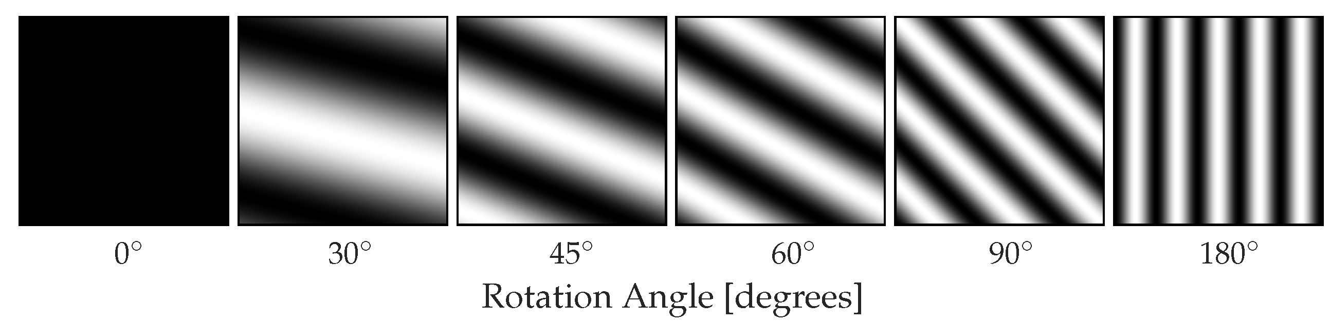
Figure 5 shows six interferograms obtained by computational simulation. The interferograms were generated by adjusting the OPD to
and changing the rotation angle from 0
to 180
with the star aligned with the optical axis. These interferograms are composed of straight fringes for which density and orientation change when the interferometer rotation-angle is changed, according to Equation (
8). The fringes are produced by the interference of the planet wavefront with itself; this confirms the planet presence. The rotation of the fringe allows for discarding several false-positives by alignment errors. The image grayscale range is adjusted to coincide its saturation level with the maximum incidance, produced by
term.
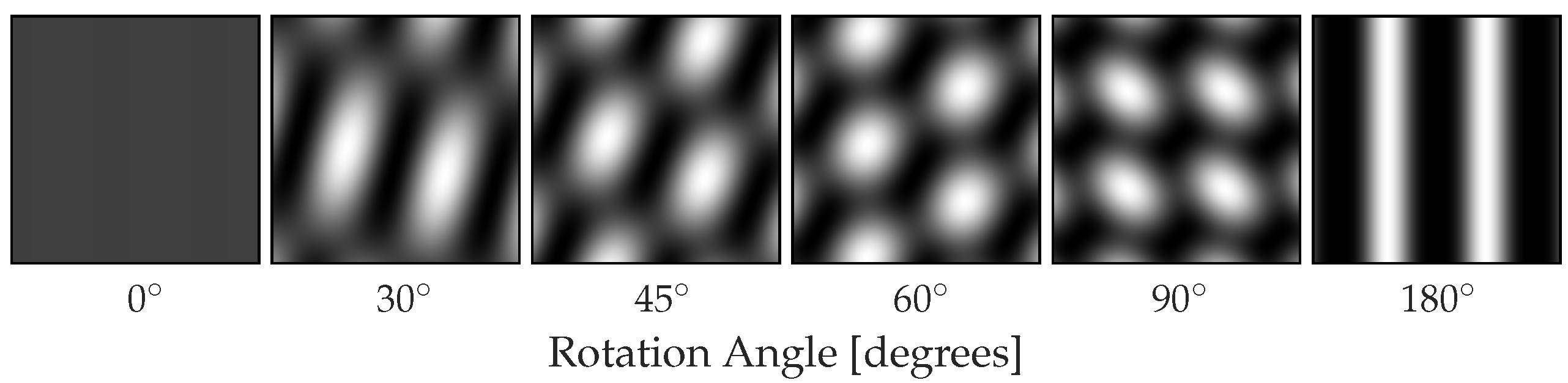
Figure 6 shows interferograms generated adjusting the OPD to
nm with the star aligned to the optical axis. These interferograms are composed by two straight fringes superposed. The fringes density and orientation changes with the interferometer rotation-angle as predicted in Equation (
8). These fringes correspond to the interference between the star and the planet. The fringes produced by the interference of the planet with itself are present; however, they are eclipsed by the brightness of star–planet fringes. The first image shows the background incidance produced by the interference of the star wavefront with its rotated version. The image grayscale is adjusted to coincide with the maximum incidance, produced by the
term. In this case, we obtain a signal gain of 4 with respect to the previous case. The gain is calculated as the difference between the minimum and the maximum incidance level of the resultant interferogram compared to the difference between the minimum and the maximum of the
term.
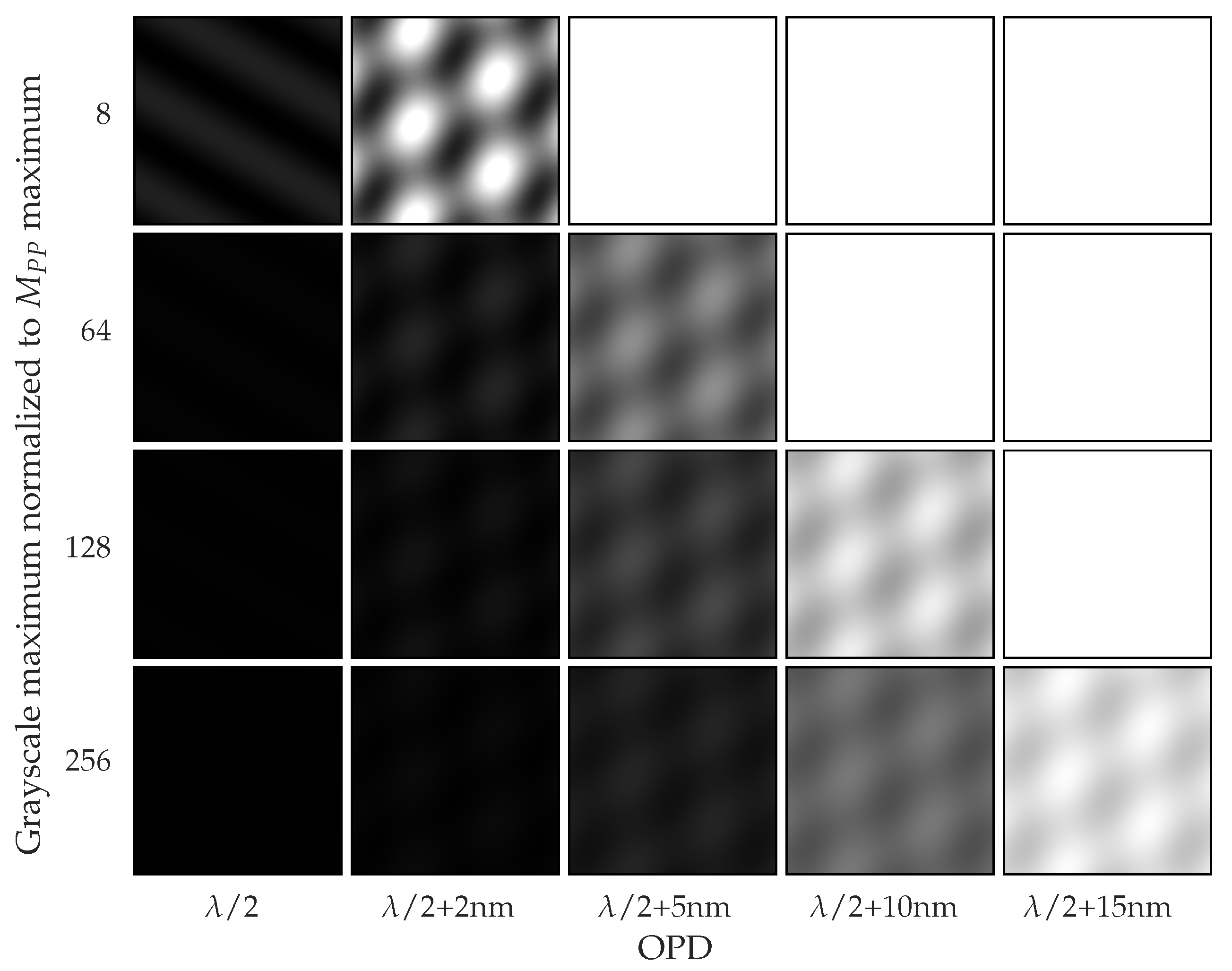
The increment in the fringe incidance in accordance with the OPD variation is showed by
Figure 7. It shows interferograms with different grayscale ranges: in the first row, the image saturation-level is 8 times the
maximum, in the second row 64 times, in the third row 128 times, and 256 times in the fourth row. The OPD is changed in each column: in the first column, the OPD is
, in the second column, the OPD is
nm, in the third column, the OPD is
nm, in the fourth column, the OPD is
nm, and, finally, in the last column, the OPD is
nm. We may observe that the fringe visibility decreases accordingly the OPD moves away
. However, the signal magnitude is increased and the pattern is still visible to the naked eye. When the OPD is
nm, the gain is 60 and the fringe visibility is 13%.
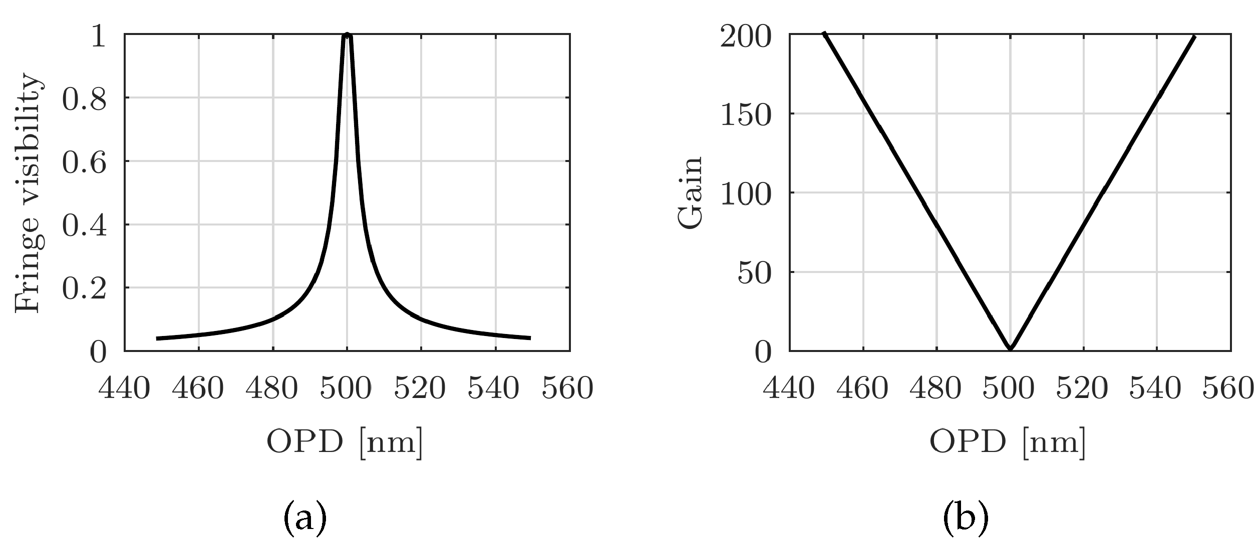
Figure 8 shows the fringe visibility and the gain versus the OPD. We may observe that the gain is increased almost linearly. In contrast, the fringe visibility decays rapidly. This behavior may confuse and erroneously discourage this technique because the visibility had a small value. However, the signal may be easily distinguishable, and the gain improvement is substantial as shown in
Figure 7. Additionally, we may observe that the fringe visibility reduction is slow after 20 nm away
, and the signal gain continues to increase at the same rate.


 ,
, 


