Learning-Based Dissimilarity for Clustering Categorical Data

Abstract

Comparing data objects is at the heart of machine learning. For continuous data, object dissimilarity is usually taken to be object distance; however, for categorical data, there is no universal agreement, for categories can be ordered in several different ways. Most existing category dissimilarity measures characterize the distance among the values an attribute may take using precisely the number of different values the attribute takes (the attribute space) and the frequency at which they occur. These kinds of measures overlook attribute interdependence, which may provide valuable information when capturing per-attribute object dissimilarity. In this paper, we introduce a novel object dissimilarity measure that we call Learning-Based Dissimilarity, for comparing categorical data. Our measure characterizes the distance between two categorical values of a given attribute in terms of how likely it is that such values are confused or not when all the dataset objects with the remaining attributes are used to predict them. To that end, we provide an algorithm that, given a target attribute, first learns a classification model in order to compute a confusion matrix for the attribute. Then, our method transforms the confusion matrix into a per-attribute dissimilarity measure. We have successfully tested our measure against 55 datasets gathered from the University of California, Irvine (UCI) Machine Learning Repository. Our results show that it surpasses, in terms of various performance indicators for data clustering, the most prominent distance relations put forward in the literature.

1. Introduction

Comparing data objects is at the heart of machine learning, for most data mining and knowledge discovery techniques rely on a way to measure the similarity of objects. For continuous data, object similarity is usually fixed to some object distance relation (e.g., Minkowski [1]); however, for categorical data, there is not a universally accepted relation. This is because the values that a categorical attribute may take can be ordered in several different ways.

Most of the existing similarity measures characterize the distance among the values an attribute may take using precisely the number of different values the attribute takes (the attribute space) and the frequency at which they occur. This approach yields three main kinds of distance relation. One is based on probability, which includes similarity relations that are information-theoretic centered, for example [2,3,4,5,6]; the next is based on the attribute space, for example [7,8,9]; and the other amounts to a specialization of a standard measure, such as Euclidean or Manhattan distance. All these measures overlook attribute interdependence, which, as noted in [10], may provide valuable information when capturing per-attribute object similarity.

In this paper, we introduce a novel object dissimilarity measure that we call Learning-Based Dissimilarity, for comparing categorical data. (In passing, we note that per-attribute value dissimilarity is a complementary relation of similarity. In our discussion, we will switch freely between these two notions, according to the context.) This measure characterizes the dissimilarity between two categorical values of a given attribute in terms of a proportion as to how likely such values are confused or not when the remaining attributes are used to predict them. To that end, we provide an algorithm that, given a target attribute, first learns a classification model in order to compute a confusion matrix for the attribute. Then, our method transforms the confusion matrix into a per-attribute dissimilarity measure. Iterating on each attribute for a given dataset, our method builds the complete dissimilarity measure for all categorical data in the set.

We have extensively experimented with Learning-Based Dissimilarity in the context of clustering. We have successfully tested our measure against 55 datasets gathered from the UCI Machine Learning Repository [11]. Our results show that it surpasses, in terms of various performance indicators for data clustering, the most prominent distance relations put forward in the literature, namely: Goodall, Gambaryan, Eskin, Manhattan, Euclidean, Lin, occurrence frequency, and inverse occurrence frequency.

Our results suggest that one should attempt to exploit any correlation among object attributes to characterize object dissimilarity in the context of categorical data. This opens two new lines of investigation, namely: the discovery of new inter-attribute comparison measures and the discovery of novel similarity measures that combine both inter- and intra-attribute comparison measures.

In summary, our contributions are as follows.

• We identify a means of defining a relation for categorical data (dis)similarity, which captures a meaningful characterization of value distance in terms of inter-attribute value dependency.
• We provide an algorithm that, given a target attribute, computes a per-attribute similarity relation, using a prediction relation provided by the values of other object attributes in a given entire dataset.
• We open further lines of investigation to study similarity relations that may simultaneously exploit inter-attribute value dependency and intra-attribute value space.

The remainder of this paper is organized as follows. Section 2 gives an overview of the most popular similarity measures for categorical data and also introduces symbols and notation. Section 3 is the core of our paper, as it introduces Learning-Based Dissimilarity and provides an example application of it. Then, Section 4 describes our experimental framework and Section 5 outlines our main findings, including an analysis of them. Finally, Section 6 gives an overview of the conclusions drawn from this research and provides directions for further research.

2. Related Work

The aim of this section is twofold. First, it provides a general discussion of the rationale behind both existing similarity relations and a new interpretation where the distance among two values that a categorical piece of data may take can be modeled taking into account the entire context of a dataset, as opposed to only the composition of the image of the data. Second, this section gives a definition of the similarity measures that we have used for comparison purposes throughout our study.

2.1. An Account for Per-Attribute Similarity Measures

Let $a_k$ be an arbitrary categorical attribute that may take $v_k$ different values. Then, existing similarity relations are defined so as to exploit three key observations. First, two distinct attribute values model two distinctive aspects of the real world and should be considered dissimilar events. Second, the larger $v_k$, the number of distinct values $a_k$ may take, the less separable the values are, and so they should be deemed to be more similar. Third, the more similar the frequency at which two attribute values occur, the more dissimilar they become. These observations can be used to yield a well-defined similarity relation; however, the output relation may be anything but intuitive. This is because these relations characterize attribute value similarity in terms of the structure of that attribute space. However, it is difficult to argue that such structure captures a similarity meaning among the distinct values that the attribute takes. Further, the structure of the attribute space is something that can be manipulated externally; that is, we may induce a different similarity relation just by changing the construction of the dataset, making the entire process error-prone.

By way of comparison, our approach to per-attribute similarity considers that every element in a dataset corresponds to a reading of a system or an aspect of the world. Each reading ought to be consistent, even though we do not neglect or overlook the possibility of a noisy observation. Typically, an object (that is, an observation about the world) is given in terms of the readings of several sensors, inputs, or other attributes, but together, across the dataset, the attribute values are in a way coherent; one would not expect to watch a Jaguar jumping over a hill in Juneau. If one is able to accurately predict two distinct attribute values from the other attributes’ values in a number of objects, then we deem the two target attribute values to be highly separable and thus highly dissimilar.

There are, of course, several wrinkles to reify our similarity relation. One is to identify a prediction function that suitably captures any form of inter-attribute value dependability. There are several options worth exploring, although in this paper we focus only on implementing prediction through the use of a classification ensemble. Another issue is how to map a similarity value out from a prediction function, for it has to be done in a way that correctly expresses subtle differences between attribute values. In our understanding, if two attribute values cannot be crisply separated, then we take them to be similar, for one might be taken to be a noisy capture of a reading of the other.

However, the benefit of following our approach is that a suitable prediction function gracefully degrades, yielding properties seen in an intra-attribute space similarity relation. For example, the larger the number of distinct values $a_k$ may take, the more difficult value prediction becomes, and so attribute values will be considered to be more similar to one another. In addition, in the presence of an imbalance as to the frequency at which an attribute value occurs, the more likely that attribute value will be considered similar to other attribute values of more frequent occurrence.

We believe that our paper may open several lines of investigation. One, for example, would attempt to identify better abstractions of counts of value predictions. Others would consider interesting combinations of these two approaches. We can see our approach is philosophically rather distinct in nature from previous ones.

2.2. Per-Attribute Similarity Measures for Categorical Data

According to Boriah et al. [9], there are two notions of similarity: one is neighborhood-based, and so it is used to define the neighborhood of an object; the other is instance oriented, and so it is used to compute the similarity between two object instances. As in [9], our study considers the latter notion only, for it can be thought of as being a key part to define neighborhood-based similarity.

We now introduce some notation in order to overview the types of similarity relations that will be considered in our study. Let $\mathbf{X}$ be a finite, categorical dataset, containing n objects, $\mathbf{X}=\{{\mathbf{x}}_1,\dots ,{\mathbf{x}}_n\}$. The properties of each object in $\mathbf{X}$ are described in terms of a fixed set of attributes, $A=\{a_1,\dots ,a_m\}$. Each attribute, $a_k$, is defined over an intended domain $D_k$, examples of which include $\{\mathrm{true},\mathrm{false}\}$ and $\{\mathrm{north},\mathrm{south},\mathrm{east},\mathrm{west}\}$. An instance, ${\mathbf{x}}_i$, is given by a tuple $(x_{i1}\dots ,x_{im})\in D_1\times \dots \times D_m$.

Take any two objects, ${\mathbf{x}}_i,{\mathbf{x}}_j\in \mathbf{X}$. Then, the similarity of the object pair ${\mathbf{x}}_i$ and ${\mathbf{x}}_j$, in symbols ${\mathbf{x}}_i\sim {\mathbf{x}}_j$, is defined as the pairwise similarity between the two values of both objects’ attributes [12]:

$${\mathbf{x}}_i\sim {\mathbf{x}}_j=\sum _{k=1}^m{\omega }_k\left({\mathbf{x}}_{ik}{\sim }_k{\mathbf{x}}_{jk}\right)$$

(1)

where ${\omega }_k$ stands for the weight assigned to attribute $a_k$, and where ${\sim }_k$ is the per-attribute similarity between ${\mathbf{x}}_{ik},{\mathbf{x}}_{jk}$, for some attribute $a_k\in A$, defined over $D_k$.

As in [12], our work considers ${\omega }_i=1/m,(i\in \{1,\dots ,m\})$. Now, evaluating ${\mathbf{x}}_{ik}{\sim }_k{\mathbf{x}}_{jk},(k\in D_k)$ essentially amounts to building a symmetric matrix. Let $D_k=\{a_{k1},\dots ,a_{k|D_k|}\}$, then:

$${\mathbf{x}}_{ik}{\sim }_k{\mathbf{x}}_{jk}=\left[\begin{array}{cccc}{a}_{k1}{\sim }_k{a}_{k1}& a_{k1}{\sim }_k{a}_{k2}& \dots & a_{k1}{\sim }_k{a}_{k|D_k|}\\ & a_{k2}{\sim }_k{a}_{k2}& \dots & a_{k2}{\sim }_k{a}_{k|D_k|}\\ & & \ddots & ⋮\\ & & & a_{k|D_k|}{\sim }_k{a}_{k|D_k|}\end{array}\right]$$

(2)

where, in addition, $a_{ki}{\sim }_k{a}_{kj}=0$, for all $a_{ki}\notin D_k$ and $a_{kj}\notin D_k$.

We are now ready to define the standard taxonomy (see, for example, [9,12]) for per-attribute similarity measures, which is then easily extended in the usual way to object similarity measures, see Equation (1). Based on the symmetric matrix defining ${\sim }_k$, Equation (2), the similarity measures studied in this paper can be classified as follows:

• Type DEO: those that fill the diagonal entries only (DEO); that is, similarity measures that assign a non-zero value for the similarities where a value match occurs, and a zero otherwise:

  $$\begin{array}{c}\hfill a_{ki}{\sim }_k{a}_{kj}=\left\{\begin{array}{ccc}u,& \mathrm{if}i=j& \mathrm{with}u\in [0,1]\\ 0,& \mathrm{if}i\ne j\end{array}\right.\end{array}$$
• Type OEO: those that fill the off-diagonal entries only (OEO); that is, similarity measures that assign a value of one for the similarities in which a value match occurs, and a value $u\in [0,1]$ otherwise:

  $$\begin{array}{c}\hfill a_{ki}{\sim }_k{a}_{kj}=\left\{\begin{array}{ccc}1,& \mathrm{if}i=j& \\ u,& \mathrm{if}i\ne j& \mathrm{with}u\in [0,1]\end{array}\right.\end{array}$$
• Type DOE: those that fill both diagonal and off-diagonal entries (DOE); that is, similarity measures that assign values $u,v\in [0,1]$, with $u\ne v$, when a value match or mismatch occurs:

  $$\begin{array}{c}\hfill a_{ki}{\sim }_k{a}_{kj}=\left\{\begin{array}{ccc}u,& \mathrm{if}i=j& \mathrm{with}u\in [0,1]\\ v,& \mathrm{if}i\ne j& \mathrm{with}v\in [0,1]\end{array}\right.\end{array}$$

2.3. Per-Attribute Similarity Measures Used in Our Study

In this study, for comparison purposes, we shall consider eight per-attribute similarity measures: Eskin, Lin, occurrence frequency (OF), inverse occurrence frequency (IOF), Goodall, Gambaryan, Euclidean, and Manhattan. The rationale behind our choosing is severalfold. First, we consider at least one relation for each different type DEO, OEO, and DOE: Goodall, Gambaryan, Manhattan, and Euclidean are of type DEO; Eskin, OF, and IOF are of type OEO; and Lin is of type DOE. Second, these measures are the de facto standard for comparison purposes (see, for example, [9,12]). Third, they have been extensively studied.

To provide formal definitions of these similarity measures, we first introduce more notation:

• $v_k$: the amount of distinct values the kth attribute takes in the dataset $\mathbf{X}$;
• ${\mathrm{fr}}_k\left(x\right)$, frequency in which attribute $a_k$ takes the value x in the dataset $\mathbf{X}$. Note that, in particular, ${\mathrm{fr}}_k\left(x\right)=0$ for any $x\notin D_k$;
• $\mathrm{fr}\left(x\right)$, frequency of value x in the dataset $\mathbf{X}$;
• ${Pr}_k\left(x\right)$, probability that attribute $a_k$ takes the value x in the dataset $\mathbf{X}$, given by

  $${Pr}_k\left(x\right)=\frac{{\mathrm{fr}}_k\left(x\right)}{n}$$
• ${Pr}_k^2\left(x\right)$, estimated probability that attribute $a_k$ takes the value x in the dataset $\mathbf{X}$, given by

  $${Pr}_k^2\left(x\right)=\frac{{\mathrm{fr}}_k\left(x\right)({\mathrm{fr}}_k\left(x\right)-1)}{n(n-1)}$$

We are now ready to define the similarity measures under consideration.

2.3.1. Goodall Similarity

The Goodall similarity [2], of type DEO, is defined as follows. Let ${\prec }_k$ be a partial order over $D_k$, the domain of attribute $a_k$, given as follows: $x{\prec }_k{x}^{\prime }$ if and only if $Pr\left(x\right)<Pr\left(x^{\prime }\right)$, under the proviso of $x,x^{\prime }\in D_k$. We extend ${\prec }_k$ to ${⪯}_k$ in the expected manner. Then, we define the cumulative estimated probability out of the partially ordered set of the domain of attribute $a_k$, and ${⪯}_k$, up to a value $x\in D_k$, as follows:

$$\begin{array}{c}\hfill {\displaystyle {Pr}_k^2(X⪯x)=\sum _{y\in \left\{x^{\prime }:x^{\prime }{⪯}_{k}x\right\}}{Pr}_k^2\left(y\right)}\end{array}$$

Then, Goodall is given by

$$\begin{array}{c}\hfill a_{ki}{\sim }_k{a}_{kj}=\left\{\begin{array}{cc}1-{Pr}_k^2(X\le a_{ki}),\hfill & \mathrm{if}{a}_{ki}=a_{kj}\\ 0,\hfill & \mathrm{if}{a}_{ki}\ne a_{kj}\end{array}\right.\end{array}$$

Clearly, Goodall gives a high similarity measure to objects ${\mathbf{x}}_i,{\mathbf{x}}_j\in \mathbf{X}$ if both the pairwise values of ${\mathbf{x}}_i$ and ${\mathbf{x}}_j$ are equal, and such values, with respect to the corresponding attribute, do not frequently occur in $\mathbf{X}$.

2.3.2. Gambaryan Similarity

The Gambaryan similarity measure [3], of type DEO, is defined pretty much the same as the entropy of a value x, $\mathrm{H}\left(x\right)$. Put in terms of an attribute $a_k$, we define both ${\mathrm{h}}_k\left(x\right)={Pr}_k\left(x\right){log}_2{Pr}_k\left(x\right)$ and ${\widehat{\mathrm{h}}}_k\left(x\right)=(1-{Pr}_k\left(x\right)){log}_2(1-{Pr}_k\left(x\right))$. Then, Gambaryan is given as follows:

$$\begin{array}{c}\hfill a_{ki}{\sim }_k{a}_{kj}=\left\{\begin{array}{cc}-[{\mathrm{h}}_k\left(a_{ki}\right)+{\widehat{\mathrm{h}}}_k\left(a_{ki}\right)],\hfill & \mathrm{if}{a}_{ki}=a_{kj}\\ 0,\hfill & \mathrm{if}{a}_{ki}\ne a_{kj}\end{array}\right.\end{array}$$

Unlike Goodall, Gambaryan gives a high similarity measure to objects ${\mathbf{x}}_i,{\mathbf{x}}_j\in \mathbf{X}$, if both the values of ${\mathbf{x}}_i$ and ${\mathbf{x}}_j$ are pairwise equal, and such values frequently occur in $\mathbf{X}$, with respect to the corresponding attribute.

2.3.3. Manhattan Distance

In our study, we also consider similarity measures that are standard extensions to their original definition for vectors of numbers. For example, the per-attribute Manhattan similarity measure is defined as follows:

$$a_{ki}{\sim }_k{a}_{kj}=\left\{\begin{array}{cc}1,\hfill & \mathrm{if}{a}_{ki}=a_{kj}\\ 0,\hfill & \mathrm{if}{a}_{ki}\ne a_{kj}\end{array}\right.$$

Manhattan is of type DEO and yields a number in $[0,1]$; the maximum value is obtained when the two objects under comparison are all attribute-wise equal.

2.3.4. Euclidean Distance

The Euclidean similarity measure, of type DEO, is defined as the square root of the Manhattan similarity measure. So, instead of applying Equation (1), we now have

$${\mathbf{x}}_i\sim {\mathbf{x}}_j=\sqrt{\sum _{k=1}^m{\omega }_k\left({\mathbf{x}}_{ik}{\sim }_k{\mathbf{x}}_{jk}\right)}$$

where, as before

$$a_{ki}{\sim }_k{a}_{kj}=\left\{\begin{array}{cc}1,\hfill & \mathrm{if}{a}_{ki}=a_{kj}\\ 0,\hfill & \mathrm{if}{a}_{ki}\ne a_{kj}\end{array}\right.$$

2.3.5. Eskin Similarity

The Eskin similarity measure [8], of type OEO, is given by

$$\begin{array}{c}\hfill a_{ki}{\sim }_k{a}_{kj}=\left\{\begin{array}{cc}1,\hfill & \mathrm{if}{a}_{ki}=a_{kj}\\ \frac{v_k^2}{v_k^2+2},\hfill & \mathrm{if}{a}_{ki}\ne a_{kj}\end{array}\right.\end{array}$$

It follows that Eskin deems the occurrence of different values for an attribute $a_k$ to be non-interesting, whenever that attribute takes a large amount of distinct values, $v_k$; this is because $\frac{v_k^2}{v_k^2+2}\approx 1$ if $v_k\gg 0$. In the opposite case, when the attribute takes a few values, the mismatch becomes paramount; note that for the minimum value that $v_k$ may take (namely 2), Eskin will assign $\frac{2}{3}$ to a mismatch.

2.3.6. Occurrence Frequency (OF) Similarity

OF, a similarity measure of type OEO, is defined as follows [9]:

$$\begin{array}{c}\hfill a_{ki}{\sim }_k{a}_{kj}=\left\{\begin{array}{cc}1,\hfill & \mathrm{if}{a}_{ki}=a_{kj}\\ \frac{1}{1+log\left(\frac{v_k}{{\mathrm{fr}}_k\left(a_{ki}\right)}\right)log\left(\frac{v_k}{{\mathrm{fr}}_k\left(a_{kj}\right)}\right)},\hfill & \mathrm{if}{a}_{ki}\ne a_{kj}\end{array}\right.\end{array}$$

Therefore, OF gives a high per-attribute similarity measure to a mismatch, if such values occur frequently often in $D_k$. The range of $a_{ki}{\sim }_k{a}_{kj}$, whenever $a_{ki}\ne a_{kj}$ is $\left[\frac{1}{1+{log}^2\left(n\right)},\frac{1}{1+{log}^2\left(2\right)}\right]$. The measure yields the minimum value when $a_{ki}$ and $a_{kj}$ occur only once in $\mathbf{X}$; that is, $v_k=1$ and ${\mathrm{fr}}_k\left(a_{ki}\right)={\mathrm{fr}}_k\left(a_{kj}\right)=\frac{1}{n}$. By contrast, OF yields the maximum one when $a_{ki}$ and $a_{kj}$ are the only values for $a_k$ in X and they occur with the same frequency; that is, $v_k=2$ and ${\mathrm{fr}}_k\left(a_{ki}\right)={\mathrm{fr}}_k\left(a_{kj}\right)=\frac{n}{2}$.

2.3.7. Inverse Occurrence Frequency (IOF) Similarity

The IOF similarity measure [7] is also of type OEO; it is given by

$$\begin{array}{c}\hfill a_{ki}{\sim }_k{a}_{kj}=\left\{\begin{array}{cc}1,\hfill & \mathrm{if}{a}_{ki}=a_{kj}\\ \frac{1}{1+log\left({\mathrm{fr}}_k\left(a_{ki}\right)\right)log\left({\mathrm{fr}}_k\left(a_{kj}\right)\right)},\hfill & \mathrm{if}{a}_{ki}\ne a_{kj}\end{array}\right.\end{array}$$

As the name suggests, IOF is defined in terms of inverse frequency. However, as it stands, it exploits the fact that the frequency in which attribute $a_k$ takes the value x, ${\mathrm{fr}}_k\left(x\right)$, is approximately equal to that in which x occurs in dataset $\mathbf{X}$, $\mathrm{fr}\left(x\right)$. This is, in turn, approximately equal to the frequency in which x appears, no matter how many times, in every attribute $a_k\in A$, the so-called inverse occurrence frequency of x in $\mathbf{X}$.

From the definition it follows that, unlike OF, IOF gives a low per-attribute similarity measure to a mismatch, see $log\left({\mathrm{fr}}_k\left(a_{ki}\right)\right)log\left({\mathrm{fr}}_k\left(a_{kj}\right)\right)$, whenever $a_{ki}$ and $a_{kj}$ occur frequently often in $a_k$.

2.3.8. Lin Similarity

The Lin similarity measure [4] is of type DOE and is based on information theory. It relies on the similarity theorem, which states that the similarity between x and y is given by the ratio between the information one needs to describe the commonality of x and y, and the information needed to completely describe x and y; in symbols:

$$x\sim y=\frac{log(Pr(\mathrm{common}(x,y)\left)\right)}{log(Pr(\mathrm{description}(x,y)\left)\right)}$$

For our case, when defining the per-attribute similarity measure for $a_{k,i},a_{k,j}\in D_k$, we drop off the denominator, for it is the same regardless of $a_{k,i}=a_{k,j}$ or $a_{k,i}\ne a_{k,j}$. Finally, if we define

$$\begin{array}{c}\hfill log(Pr\left(\mathrm{common}(x,y)\right))=\left\{\begin{array}{cc}log(Pr(x\mathrm{and}y\left)\right),\hfill & \mathrm{if}x=y\\ 2log(Pr(x\mathrm{or}y\left)\right),\hfill & \mathrm{if}x\ne y\end{array}\right.\end{array}$$

we then arrive at the standard formulation of the Lin similarity:

$$\begin{array}{c}\hfill a_{ki}{\sim }_k{a}_{kj}=\left\{\begin{array}{cc}2log\left({Pr}_k\left(a_{ki}\right)\right),\hfill & \mathrm{if}{a}_{ki}=a_{kj}\\ 2log({Pr}_k\left(a_{ki}\right)+{Pr}_k\left(a_{kj}\right)),\hfill & \mathrm{if}{a}_{ki}\ne a_{kj}\end{array}\right.\end{array}$$

According to [9], Lin gives a higher per-attribute similarity measure to matches on frequent values, but lower ones to mismatches on infrequent values.

We now introduce our notion of similarity.

3. Learning-Based Dissimilarity

This section is the core of this paper. We introduce a novel dissimilarity measure that we call Learning-Based Dissimilarity. The rationale behind our measure is that two object attribute values should be rendered dissimilar whenever one cannot be taken to be the other. To verify when two attribute values are not distinguishable, we exploit the fact that attributes might depend on one another. In particular, to compute Learning-Based Dissimilarity, we make a classifier to infer an attribute value using the values of the others. Two attribute values will be taken to be more similar whenever the associated classifier is more likely to misleadingly classify one of these values to be the other. Note that this implies that Learning-Based Dissimilarity is anti-symmetric. This, we believe, is crucial as it captures that many wolves can pass as a dog; this statement, however, does not reverse in general (consider, for example, a chihuahua exemplar).

3.1. Per-Attribute Learning-Based Dissimilarity

Roughly, take $\mathbf{X}$ and consider the kth attribute. Now, take $\mathbf{X}$ to be a dataset, where each element belongs to one of either of $v_k$ possible classes, one for each $D_k=\{a_{k1},a_{k2},\dots ,a_{k{v}_k}\}$. Then, train a classifier so as to infer the class $a_k$ from ${\mathbf{X}}^{\prime }$, which is as $\mathbf{X}$, except that for every ${\mathbf{x}}_i\in \mathbf{X}$, we have ${\mathbf{x}}_i^{\prime }\in {\mathbf{X}}^{\prime }$, with ${\mathbf{x}}_{\mathbf{i}}=({\mathbf{x}}_{i1},\dots ,{\mathbf{x}}_{ik},\dots ,{\mathbf{x}}_{im})$, and ${\mathbf{x}}_i^{\prime }=({\mathbf{x}}_{i1}^{\prime },\dots ,{\mathbf{x}}_{ik-1}^{\prime },{\mathbf{x}}_{ik+1}^{\prime },\dots ,{\mathbf{x}}_{im}^{\prime })$. Then, two elements, ${\mathbf{x}}_{ik}$ and ${\mathbf{x}}_{jk}$, are learning-based similar (written in symbols ${\mathbf{x}}_{ik}{\sim }_k^{\mathrm{LBS}}{\mathbf{x}}_{jk}$) if and only if:

$$\begin{array}{c}\hfill {\mathbf{x}}_{ik}{\sim }_k^{\mathrm{LBS}}{\mathbf{x}}_{jk}=\left\{\begin{array}{ccc}1,\hfill & \mathrm{if}i=j& \\ u_1>0,\hfill & \mathrm{if}i\ne j& \&\mathrm{classifier}\mathrm{often}\mathrm{confuses}i\mathrm{with}j\hfill \\ u_2<u_1\hfill & \mathrm{if}i\ne j& \&\mathrm{classifier}\mathrm{often}\mathrm{distinguishes}i\mathrm{from}j\hfill \end{array}\right.\end{array}$$

Therefore, it follows that Learning-Based Similarity is of type OEO. As expected, the Learning-Based Dissimilarity of ${\mathbf{x}}_{ik}$ and ${\mathbf{x}}_{jk}$, in symbols ${\mathrm{d}}_{\mathrm{LBD}}({\mathbf{x}}_{ik},{\mathbf{x}}_{jk})$, is given by

$${\mathrm{d}}_{\mathrm{LBD}}({\mathbf{x}}_{ik},{\mathbf{x}}_{jk})=1-{\mathbf{x}}_{ik}{\sim }_k^{\mathrm{LBS}}{\mathbf{x}}_{jk}$$

(3)

We now proceed to provide the inner procedural workings of our relation.

3.2. Learning-Based Dissimilarity, the Algorithm

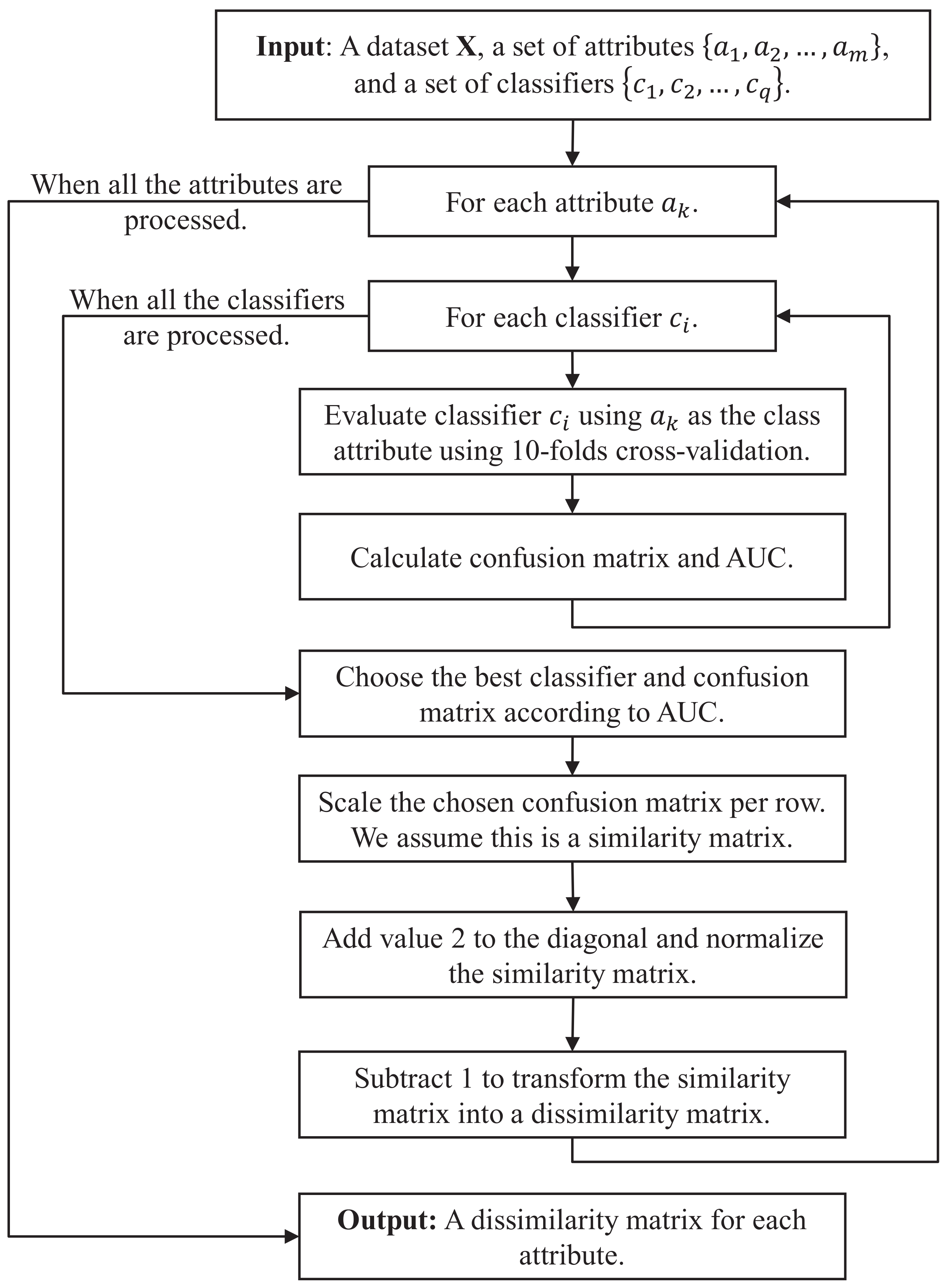
For computing per-attribute Learning-Based (Dis)similarity, we follow a two-step approach. Given $\mathbf{X}$ and a target attribute, $a_k$, in the first step, our algorithm extracts ${\mathbf{X}}^{\prime }$ and then trains a classifier for $a_k$ so as to compute a confusion matrix for it. Then, in the second step, our algorithm transforms the confusion matrix into a (dis)similarity measure. This procedure is applied repeatedly to $\mathbf{X}$, according to m, the number of attributes of each object in $\mathbf{X}$.

Figure 1 depicts a flow diagram of Learning-Based Dissimilarity. It is worth noting that, to avoid any kind of bias, in the first step (cf. inner loop), instead of using a single classifier, we rather use an ensemble of different classifiers. Then, for the attribute under consideration, we set the confusion matrix to be the one output by the classifier with the highest area under the receiver operational characteristic curve (AUC, for short). The rationale behind using a classification ensemble is as follows. Supervised classifiers make assumptions about the structure of data for a ‘correct’ generalization. We address this issue following [13], using an ensemble of distinct supervised classifiers and then applying a max combination rule. In our experimentation, we use Random Forest, Naïve Bayes, Bayesian Networks, Bagging, Simple Logistic, and KStar, as implemented in the Weka data mining tool [14].

Next, to transform the confusion matrix into a per-attribute (dis)similarity measure, we proceed as follows. Take an attribute, $a_k$, with $v_k$ different values. Then:

• Normalize each row of the confusion matrix, i.e.,

  $$\begin{array}{c}\hfill a_{ki}⟵\frac{a_{ki}}{{\sum }_{i=1}^{v_k}{a}_{ki}},(i\in \{1,\dots ,v_k\});\end{array}$$
• Set the element of the diagonal to be equal to one $a_{kk}⟵1$; and
• Normalize the rest of the row elements again as follows:

  $$\begin{array}{c}\hfill a_{ki}⟵\frac{a_{ki}}{3},(i\ne k,i\in \{1,\dots ,v_k\});\end{array}$$

With this, we obtain a similarity matrix for $a_k$; to transform it into a dissimilarity matrix, we simply let $a_{ki}⟵1-a_{ki},(i,k\in \{1,\dots ,v_k\})$. We apply this procedure, repeatedly, for each attribute in $\{a_1,\dots ,a_m\}$.

As expected, to compute Learning-Based Similarity, we apply Equation (1), accordingly:

$$\begin{array}{c}\hfill {\mathbf{x}}_i{\sim }^{\mathrm{LBS}}{\mathbf{x}}_j=\sum _{k=1}^m{\omega }_k\left({\mathbf{x}}_{ik}{\sim }_k^{\mathrm{LBS}}{\mathbf{x}}_{jk}\right)\end{array}$$

where, for now, we have set ${\omega }_k=1$, for $k\in \{1,\dots ,m\}$. In the remainder of this section, we show an example application of Learning-Based Similarity.

3.3. Learning-Based Dissimilarity, a Working Example

Consider Balloons, one of the datasets available at the UCI Machine Learning Repository [11]. A snapshot of this dataset appears in

Table 1. A snapshot of the Balloons Dataset. We omitted the class attribute since it is not used for clustering.

Color	Size	Act	Age
YELLOW	SMALL	STRETCH	CHILD
YELLOW	SMALL	DIP	ADULT
YELLOW	SMALL	DIP	CHILD
YELLOW	SMALL	DIP	CHILD
YELLOW	LARGE	STRETCH	ADULT
YELLOW	LARGE	STRETCH	CHILD
YELLOW	LARGE	DIP	ADULT
YELLOW	LARGE	DIP	CHILD
YELLOW	LARGE	DIP	CHILD
PURPLE	SMALL	STRETCH	ADULT
PURPLE	SMALL	STRETCH	CHILD
…	…	…	…

. In this case, $A=\{\mathbf{Color},\mathbf{Size},\mathbf{Act},\mathbf{Age}\}$; then, consider that we are to compute the per-attribute Learning-Based Similarity measure of Color.

First, we train our ensemble of classifiers to learn how to predict Color out of objects from Balloons, containing Size, Age and Act only. Having done so, we compute the AUC and then apply the max rule on AUC in order to identify the classifier that better separates Color. In this case, SimpleLogistic happens to output the highest AUC (0.75); the corresponding confusion matrix is shown in

Table 2. Confusion matrix associated with the classifier that rendered the highest area under the receiver operational characteristic curve (AUC).

Color	Yellow	Purple
yellow	7	3
purple	2	9

. This completes the first step of our algorithm (cf. Figure 1).

To transform the output confusion matrix into a similarity measure, we execute the three transformations of the second step of our algorithm, as shown in

Table 3. An example application of the second step of per-attribute learning-based similarity.

Color	Yellow	Purple
(a)
yellow	0.70	0.30
purple	0.18	0.81
(b)
yellow	1.00	0.30
purple	0.18	1.00
(c)
yellow	1.00	0.10
purple	0.06	1.00

. This completes the second step, and the sub-table (c) of Table 3 is the per-attribute Learning-Based Similarity of Color. This process is applied on the remaining attributes, namely: Size, Age and Act.

Now, consider objects ${\mathbf{x}}_1$ and ${\mathbf{x}}_2$, given by:

$$\begin{array}{ccc}\hfill {\mathbf{x}}_1& =& \langle \mathrm{yellow},\mathrm{large},\mathrm{small},\mathrm{adult}\rangle \hfill \\ \hfill {\mathbf{x}}_2& =& \langle \mathrm{purple},\mathrm{small},\mathrm{small},\mathrm{adult}\rangle \hfill \end{array}$$

Then, assuming $\mathrm{large}{\sim }_{\mathbf{Size}}^{\mathrm{LBS}}\mathrm{small}=0.15$, clearly:

$$\begin{array}{ccc}\hfill {\mathbf{x}}_1{\sim }^{\mathrm{LBS}}{\mathbf{x}}_2& =& 0.10+0.15+1+1=2.25\mathrm{and}\mathrm{conversely}\hfill \\ \hfill {\mathrm{d}}_{\mathrm{LBD}}({\mathbf{x}}_1,{\mathbf{x}}_2)& =& 0.90+0.85+0+0=1.75\hfill \end{array}$$

This completes our description of Learning-Based Similarity. In what follows, we describe an experimental analysis of this similarity measure.

4. Experimental Framework

We now describe our experimental framework, as well as the results we have obtained throughout our investigation. Since, in our study, we have chosen to use clustering as the data mining task for evaluating Learning-Based Dissimilarity, we have set KMeans++ [15] to be our basis clustering algorithm. The rationale behind this selection decision is that KMeans++ is guaranteed to find a solution that is competitive to the optimal standard KMeans solution, which is the most popular clustering algorithm.

We have modified KMeans++ so as to make it parametric of a similarity (dissimilarity) relation (the source code for our proposal is available at https://github.com/edjacob25/DissimilarityMeasures, accessed on 13 April 2021). We considered nine different relations, including learning-based, yielding nine algorithm variants. We made each KMeans++ variant run in 55 datasets, fixing k, the number of clusters to be formed, according to that of the classes provided in the corresponding dataset (the source code for batch processing is available at https://github.com/edjacob25/DissimilarityAnalysis, accessed on 13 April 2021). To compare the behavior of each variant, and hence of the corresponding similarity relation, we selected the external quality indexes F-measure [16] and Adjusted Rand Index [17] as the performance measures (the source code for computing the performance measures is available at https://github.com/edjacob25/MeasuresComparator, accessed on 13 April 2021). We confirmed our results, to be discussed in the next section, using a statistical hypothesis test.

4.1. Cluster Analysis and Datasets

For comparatively evaluating Learning-Based Dissimilarity, we chose cluster analysis, although other data mining tasks, such as anomaly detection, could have been chosen. Since the behavior of a similarity relation affects the output of, but does not depend on, the cluster analysis technique, we picked KMeans++ [15]. The rationale behind this decision is that KMeans++ is, perhaps, the most popular clustering algorithm, for it has been thoroughly studied [18], and has found a number of applications. The key problem with KMeans++ is that it needs to be given k, the target number of problems to be found. However, in our case, this is not a problem, since, as shall be described later, we have turned a classification problem into a clustering one, and so each dataset contains both objects and their intended class, and so is taken as the ground truth.

We used 55 datasets collected from the UCI Machine Learning Repository [11]. Our datasets were split into two groups. The first group contains 26 datasets, where each object’s properties were originally described using only categorical attributes. The second group, however, contains 29 datasets that were artificially made to satisfy the above property; put differently, every object in a dataset of this kind is as it was originally asserted, except that we have removed from it any attribute that is not categorical. The rationale behind this pre-processing decision is to get away from whatever possible negative impact there may be for these kinds of variable in our results.

Table 4. Datasets, as well as some characteristics thereof, used in our experimentation. They were all taken from the UCI Machine Learning Repository [11]. Columns #Ob and #Ft, respectively, stand for number of objects and number of categorical features.

Dataset Name	#Ft	#Ob	Dataset Name	#Ft	#Ob
allbp_complete	17	3772	drug_consumption_Mushrooms	6	1885
arrhythmia	74	452	drug_consumption_Nicotine	6	1885
australian	9	690	drug_consumption_Semer	6	1885
balloons	5	20	drug_consumption_VSA	6	1885
breast-cancer	10	286	hayes-roth	5	160
car	7	1728	hcc	28	165
cervical_cancer_biopsy	21	858	hiv-1	9	6590
cervical_cancer_cytology	21	858	kr-vs-kp	37	3196
cervical_cancer_hinselmann	21	858	lenses	5	24
cervical_cancer_schiller	21	858	lung-cancer	57	32
chess	37	3196	lymphography	19	148
crx	10	690	molecular_Promoter	58	106
diagnosis1	6	120	monks-1	7	556
diagnosis2	6	120	mushroom	23	8125
drug_consumption_Alcohol	6	1885	nursery	9	12,960
drug_consumption_Amphet	6	1885	postoperative-patient-data	9	90
drug_consumption_Benzos	6	1885	primary-tumor	18	339
drug_consumption_Ca	6	1885	shuttle-landing-control	7	16
drug_consumption_Cannabis	6	1885	solar-flare1	13	324
drug_consumption_Choc	6	1885	solar-flare2	13	1067
drug_consumption_Coke	6	1885	soybean-l	36	683
drug_consumption_Crack	6	1885	soybean-s	36	47
drug_consumption_Ecstasy	6	1885	spect	23	267
drug_consumption_Heroin	6	1885	splice	61	3190
drug_consumption_Ketamine	6	1885	sponge	45	76
drug_consumption_LSD	6	1885	tic-tac-toe	10	958
drug_consumption_Legalh	6	1885	vote	17	435
drug_consumption_Meth	6	1885

lists the datasets used in our investigation, together with key properties thereof.

4.2. Evaluation Protocol

Our evaluation protocol was as follows. First, remove the class label from every object in the given dataset, D, and set k, in KMeans++, to the original number of classes in D. Then, execute nine KMeans++ variants (one for each dissimilarity measure) on the 55 datasets. Next, for each executing output, compute the F-Measure and Adjusted Rand Index comparing the output clusters against the classes annotated in the original dataset. Finally, form a rank per dataset, out of these performance results, and compute the average output performance per algorithm.

As is known, the F-measure [19] is a combination of precision and recall, ranging from 0 (no matching pair of sets of clusters, in our case) to 1 (two identical sets of clusters). Hence, for a given dataset, the closer to 1 the F-measure associated with a KMeans++ variant run, the higher that variant’s rank. When calculating an F-Measure, we conducted a pairwise comparison between the original dataset and an output clustering. We are not required to have groups in the same order to obtain an accurate result and get away from problems in relation to cluster size.

The Adjusted Rand Index [17] is a measure used to compute the similarity between two given partitions (clusterings) for a set of elements. It is much stricter than F-measure, as it requires the two clusterings to be practically equal for a high measure (one).

To assess whether the population’s mean ranks of two given matched variants’ performance outputs had a significant difference, we used a statistical test, namely Wilcoxon, as described in [20], with a significance level of $0.05$. Following this proposed evaluation protocol, the best possible outcome for a given algorithm is to have an average rank of 1, which would indicate that the algorithm indisputably obtained first place in all datasets. If, in addition to this, the result for that algorithm has a p-value less than 0.05, then it would indicate that it is significantly better than the rest.

In what follows, we overview our main findings and discuss their relative significance.

5. Findings and Discussion

In our study, we used KMeans++ [15], as implemented in the Weka toolbox for machine learning and data science [21]. We slightly modified it so that, apart from k (the target number of clusters to form), it is given the dissimilarity relation as an input parameter. For each dissimilarity measure, we executed KMeans++ in all datasets, as explained previously, and computed the F-measure and Adjusted Rand Index. In passing, we note that, on any application of KMeans++, we used inputting; that is, for every dataset, any time we found that a value was missing for an object attribute, we set that value to be the mode of that object attribute.

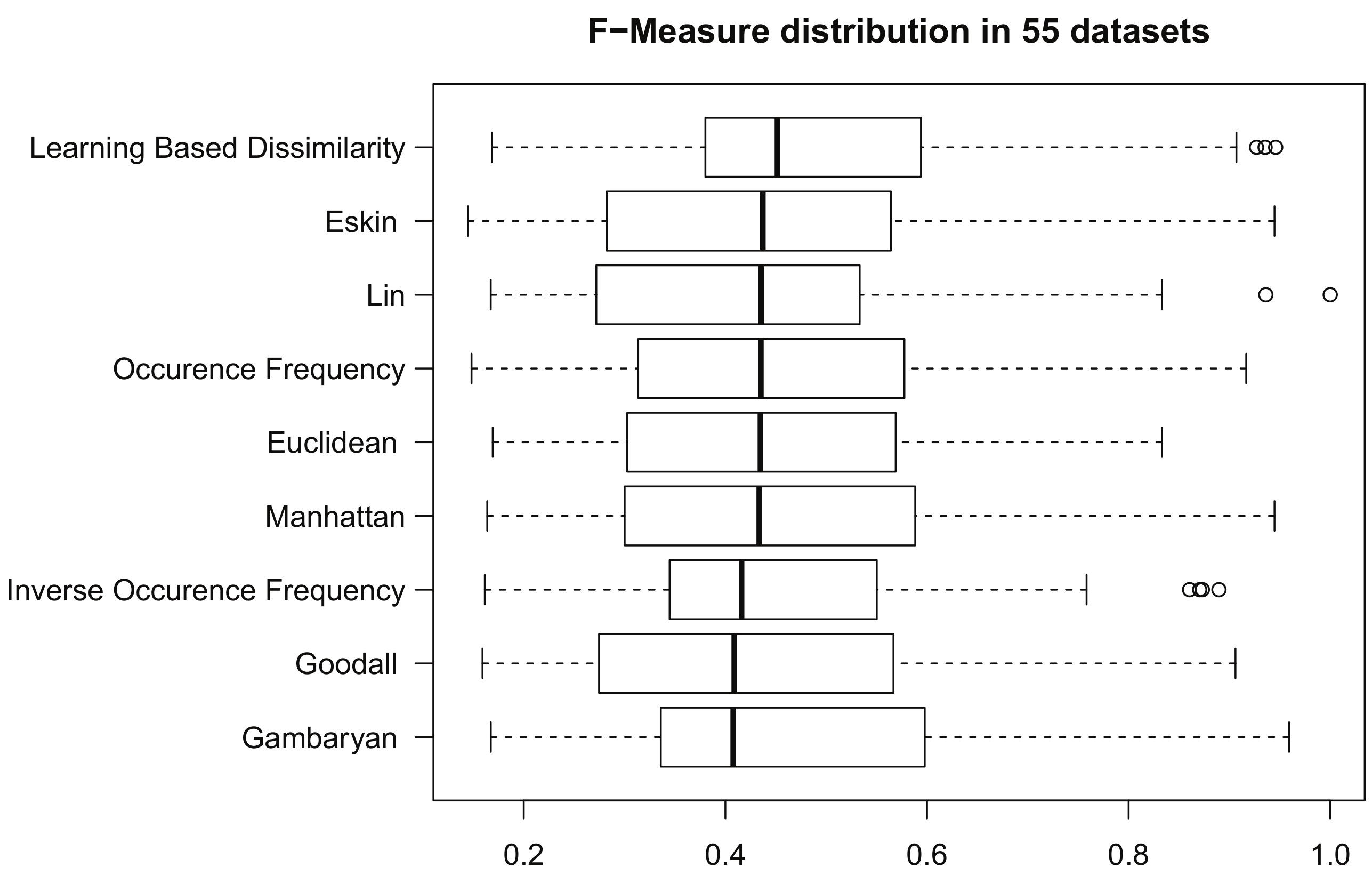
Figure 2 provides, via a box plot, a graphical description for each group of F-measures, one for every dissimilarity relation under study. In general, the greater the median of a group of F-measures, the better the associated dissimilarity relation; a similar remark applies when the size of the box is short and when the box appears closer to the right-hand side of the figure. Note how, in particular, Learning-Based Dissimilarity appears right at the top of the figure and most to the right. While this looks like a good first impression for our proposed method, we must stand on a sound, statistical method if we are to draw strong conclusions.

We used the Wilcoxon signed-rank test [22] to conduct a one-to-one comparison of Learning-Based Dissimilarity against all the other dissimilarity measures under investigation.

Table 5. Statistical results, according to F-measure [16], for KMeans++ using all the dissimilarity measures, considering all the tested datasets. The last column corresponds to the p-value obtained when comparing Learning-Based Dissimilarity against the other dissimilarity measures using the Wilcoxon signed-rank test [22]. The results are sorted from top to bottom in descending order of the associated F-measure group median.

Dissimilarity	Median F-Measure	Standard Deviation	p-Value
Learning-Based Dissimilarity	0.4516	0.1780	-
Eskin	0.4371	0.2074	0.0001
Lin	0.4353	0.2028	<0.0001
Occurrence Frequency	0.4352	0.1893	<0.0001
Euclidean	0.4347	0.1754	<0.0001
Manhattan	0.4335	0.2007	<0.0001
Inverse Occurrence Frequency	0.4160	0.1749	<0.0001
Goodall	0.4088	0.1760	<0.0001
Gambaryan	0.4077	0.2008	0.0266

summarizes our comparison results: on each row, we display a dissimilarity measure, the median, and the standard deviation of the group of F-measures output by KMeans++ for it, and the p-value output by the Wilcoxon signed-rank test, rejecting the null hypothesis. From this, we conclude that the results of K-Means++ are significantly better when using Learning-Based Dissimilarity according to F-measure.

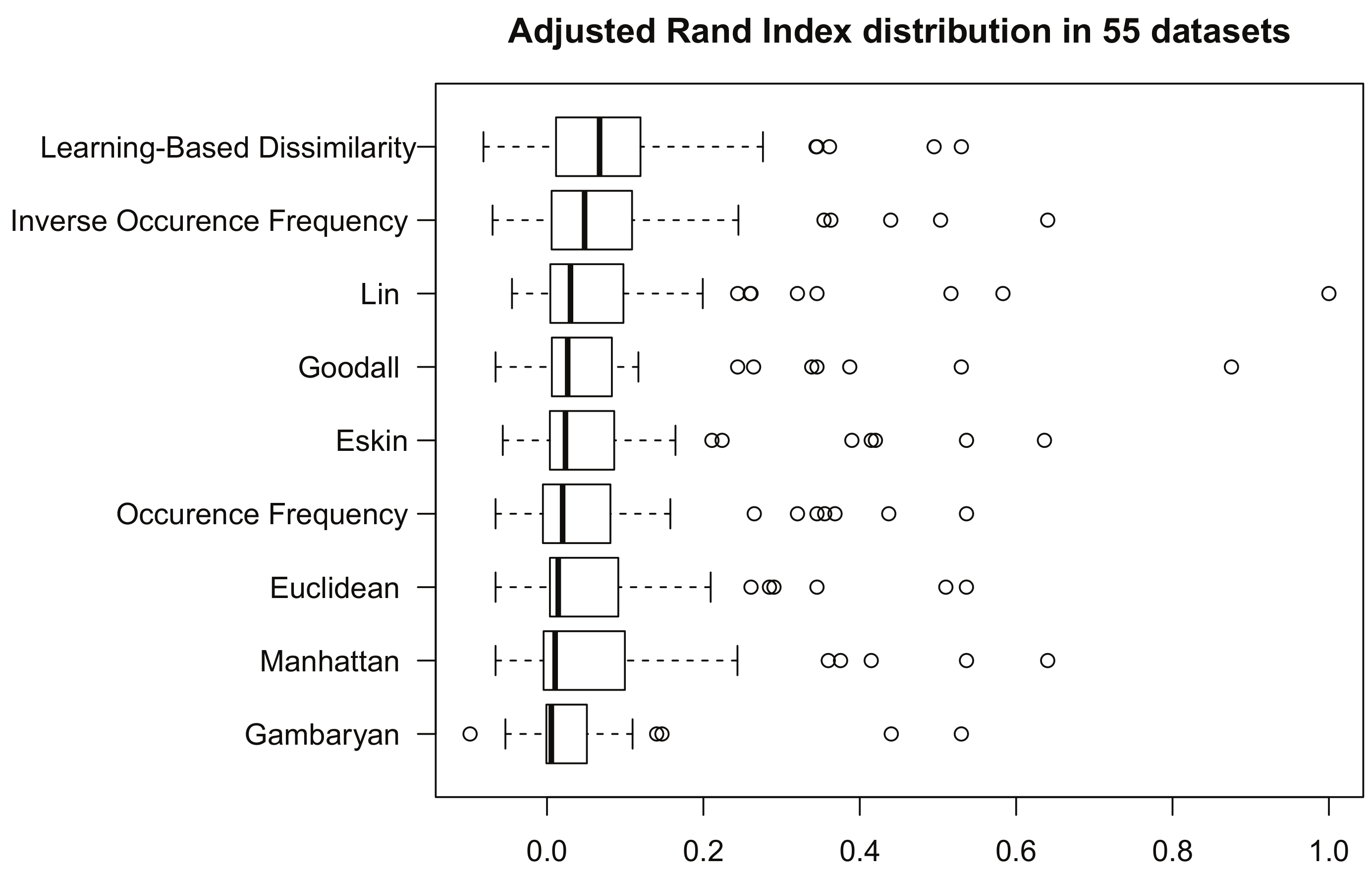
In an attempt to show that the above result holds independently of what performance measure is used, we ran a similar experiment but this time using the Adjusted Rand Index [17]. As in Figure 2, Figure 3 provides a box plot for each group of Adjusted Rand Index measures, one for every dissimilarity relation under study. Boxes are to be compared similarly as before. Again, note how, in particular, Learning-Based Dissimilarity appears right at the top of the figure and most to the right. In addition, we proceed similarly relying on the statistical method so as to draw strong conclusions.

Table 6. Statistical results, according to Adjusted Rand Index [17], for KMeans++ [15] using all the dissimilarity measures, considering all the tested datasets. The last column corresponds to the p-value obtained when comparing our proposal (Learning-Based Dissimilarity) with the other dissimilarity measures using the Wilcoxon signed-rank test [22]. The results are sorted from top to bottom in descending order of the median.

Dissimilarity	Median Adjusted Rand Index	Standard Deviation	p-Value
Learning-Based Dissimilarity	0.0672	0.1288	-
Inverse Occurrence Frequency	0.0480	0.1359	0.8525
Lin	0.0300	0.1779	0.1779
Goodall	0.0264	0.1611	0.0162
Eskin	0.0235	0.1431	0.0096
Occurrence Frequency	0.0199	0.1299	0.0048
Euclidean	0.0143	0.1236	0.0002
Manhattan	0.0103	0.1440	0.0020
Gambaryan	0.0055	0.0992	0.0007

summarizes our comparison results: on each row, we display a dissimilarity measure, the median, and the standard deviation of the group of Adjusted Rand Index measures output by KMeans++ for it, and the p-value output by the Wilcoxon signed-rank test. These results indicate no evidence supporting our proposal’s statistically significant difference compared to inverse occurrence frequency and Lin, but our proposal exhibits a higher median. With this, we provide further evidence that Learning-Based Dissimilarity is a better relation for clustering categorical values using KMeans++.

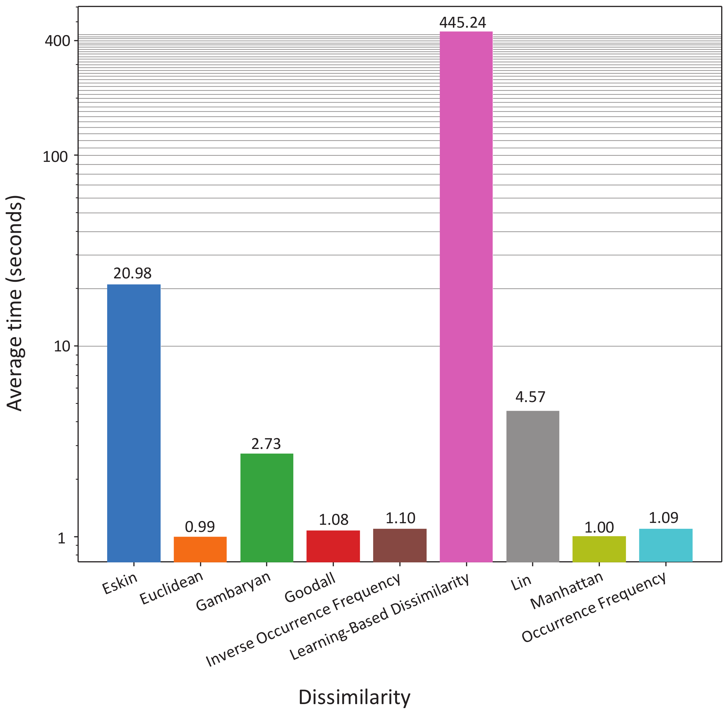
Learning-based dissimilarity, as it stands, is time-consuming, for we are required to learn the dissimilarities for the categorical values. Recall that this process involves performing cross-validation with several supervised classifiers, and this is a time-consuming task. Figure 4 shows that our proposal is, on average, between two and one orders of magnitude slower than the rest of the dissimilarity measures. From these results, we suggest performing undersampling before computing Learning-Based Dissimilarity on large datasets.

6. Conclusions

In conclusion, in this paper, we have seen how to characterize the similarity of the values of a categorical attribute through the correlation each of these attribute categories maintains with the other attributes of all the objects of a dataset. Further, we have seen that this attribute correlation can be learnt via supervised classification. We have shown that by exploiting such attribute correlation one can induce a similarity relation, which helps distinguish better what cluster one object should be associated with. We believe that our similarity relation can help similarly in other machine learning tasks, such as classification, knowledge discovery, etc.

We have shown that Learning-Based Dissimilarity outperforms, in terms of various performance indicators for data clustering, relevant distance relations that are popular in the literature. This result can be explained by the fact that existing similarity relations compute the similarity between attribute values in terms of the structure of the space of such target attributes. However, this sort of syntactic notion of similarity may not be meaningful and it is open to external manipulation, for one can easily change the composition of a dataset by simply changing some of its constituents.

We have turned the computation of inter-attribute value dependency into a classification task, where one makes use of the information provided by other attributes to predict the values of a target attribute. However, there are other ways of reifying value prediction. In addition, as mentioned previously, our approach is at least one order of magnitude more computationally expensive than standard approaches for computing per-attribute dissimilarity, and one should strive towards achieving more efficient means.

We believe that this research opens up further avenues of investigation that are worth exploring. First, one might find other ways of capturing and using attribute dependency (for example, through an attribute selection mechanism). Second, one might find new and more precise means of combining the use of attribute dependency and the underlying structure of the space of a target attribute.

References

- Merigó, J.M.; Casanovas, M. A New Minkowski Distance Based on Induced Aggregation 342 Operators. Int. J. Comput. Intell. Syst. 2011, 4, 123–133. [Google Scholar] [CrossRef]
- Goodall, D.W. A new similarity index based on probability. Biometrics 1966, 22, 882–907. [Google Scholar] [CrossRef]
- Gambaryan, P. A mathematical model of taxonomy. Izvest. Akad. Nauk Armen. SSR 1964, 17, 47–53. [Google Scholar]
- Lin, D. An Information-Theoretic Definition of Similarity. In Proceedings of the 15th International Conference on Machine Learning. Morgan Kaufmann, Madison, WI, USA, 24–27 July 1998; pp. 296–304. [Google Scholar]
- Jia, H.; Cheung, Y.; Liu, J. A New Distance Metric for Unsupervised Learning of Categorical Data. IEEE Trans. Neural Netw. Learn. Syst. 2016, 27, 1065–1079. [Google Scholar] [CrossRef] [PubMed]
- Zhang, Y.; Cheung, Y.; Tan, K.C. A Unified Entropy-Based Distance Metric for Ordinal-and-Nominal-Attribute Data Clustering. IEEE Trans. Neural Netw. Learn. Syst. 2020, 31, 39–52. [Google Scholar] [CrossRef] [PubMed]
- Church, K.W.; Gale, W.A. Inverse Document Frequency (IDF): A Measure of Deviations from Poisson. In Proceedings of the Third Workshop on Very Large Corpora, VLC@ACL 1995, Cambridge, MA, USA, 30 June 1995. [Google Scholar]
- Eskin, E.; Arnold, A.; Prerau, M.J.; Portnoy, L.; Stolfo, S.J. A Geometric Framework for Unsupervised Anomaly Detection. In Applications of Data Mining in Computer Security; Advances in Information Security; Barbará, D., Jajodia, S., Eds.; Springer: Berlin/Heidelberg, Germany, 2002; pp. 77–101. [Google Scholar] [CrossRef]
- Boriah, S.; Chandola, V.; Kumar, V. Similarity Measures for Categorical Data: A Comparative Evaluation. In Proceedings of the SIAM International Conference on Data Mining, SDM, Atlanta, GA, USA, 24–26 April 2008; pp. 243–254. [Google Scholar] [CrossRef] [Green Version]
- Zhang, Y.; Cheung, Y. An Ordinal Data Clustering Algorithm with Automated Distance Learning. In Proceedings of the AAAI Conference on Artificial Intelligence, New York, NY, USA, 7–12 February 2020; pp. 6869–6876. [Google Scholar]
- Frank, A.; Asuncion, A. UCI Machine Learning Repository: School of Information and Computer Science; University of California: Irvine, CA, USA, 2010; Volume 213, Available online: http://archive.ics.uci.edu/ml (accessed on 13 April 2021).
- Dos Santos, T.R.L.; Zárate, L.E. Categorical data clustering: What similarity measure to recommend? Expert Syst. Appl. 2015, 42, 1247–1260. [Google Scholar] [CrossRef]
- Rodríguez-Ruiz, J.; Medina-Pérez, M.A.; Gutiérrez-Rodríguez, A.E.; Monroy, R.; Terashima-Marín, H. Cluster validation using an ensemble of supervised classifiers. Knowl. Based Syst. 2018, 145, 134–144. [Google Scholar] [CrossRef]
- Hall, M.; Frank, E.; Holmes, G.; Pfahringer, B.; Reutemann, P.; Witten, I.H. The WEKA data mining software: An update. ACM SIGKDD Explor. Newsl. 2009, 11, 10–18. [Google Scholar] [CrossRef]
- Arthur, D.; Vassilvitskii, S. k-means++: The Advantages of Careful Seeding. In Proceedings of the Eighteenth Annual ACM-SIAM Symposium on Discrete Algorithms, New Orleans, LA, USA, 7–9 January 2007; pp. 1027–1035. [Google Scholar]
- Hand, D.; Christen, P. A note on using the F-measure for evaluating record linkage algorithms. Stat. Comput. 2018, 28, 539–547. [Google Scholar] [CrossRef] [Green Version]
- Hubert, L.; Arabie, P. Comparing partitions. J. Classif. 1985, 2, 193–218. [Google Scholar] [CrossRef]
- Jain, A.K. Data Clustering: 50 Years Beyond K-means. Pattern Recognit. Lett. 2010, 31, 651–666. [Google Scholar] [CrossRef]
- Amigó, E.; Gonzalo, J.; Artiles, J.; Verdejo, F. A comparison of extrinsic clustering evaluation metrics based on formal constraints. Inf. Retr. 2009, 12, 461–486. [Google Scholar] [CrossRef] [Green Version]
- Demšar, J. Statistical Comparisons of Classifiers over Multiple Data Sets. J. Mach. Learn. Res. 2006, 7, 1–30. [Google Scholar]
- Witten, I.H.; Frank, E.; Hall, M.A.; Pal, C.J. Data Mining: Practical Machine Learning Tools and Techniques; Morgan Kaufmann: Burlington, MA, USA, 2016. [Google Scholar]
- Derrac, J.; García, S.; Molina, D.; Herrera, F. A practical tutorial on the use of nonparametric statistical tests as a methodology for comparing evolutionary and swarm intelligence algorithms. Swarm Evol. Comput. 2011, 1, 3–18. [Google Scholar] [CrossRef]
Figure 1.
Flow diagram for the procedure of computing Learning-Based Dissimilarity.
Figure 2.
Box and whisker diagrams of all groups of F-measures [16]. Each F-measure group is associated with a dissimilarity measure and gathers the output of KMeans++ [15] having made a run on every dataset selected for our experimentation. Box and whisker diagrams are shown following a descending ordering, considering the associated F-measure median.
Figure 3.
Box and whisker diagram according to Adjusted Rand Index [17], for KMeans++ [15] using all the dissimilarity measures, considering all the tested datasets. The results are sorted from top to bottom in descending order of the median.
Figure 4.
Average time of clustering with KMeans++ [15] using all the dissimilarity measures, considering all the tested datasets. The vertical axis is on a logarithmic scale.