
Intelligent Scheduling with Reinforcement Learning


1
ISRC—Interdisciplinary Studies Research Center, 4200-072 Porto, Portugal
2
Institute of Engineering—Polytechnic of Porto (ISEP/P.PORTO), 4200-072 Porto, Portugal
3
INOV—Instituto de Engenharia de Sistemas e Computadores Inovação, 1000-029 Lisboa, Portugal
4
INESC TEC and University of Trás-os-Montes and Alto Douro (UTAD), 5000-801 Vila Real, Portugal
5
LEMA—Laboratory for Mathematical Engineering, 4200-072 Porto, Portugal
*
Author to whom correspondence should be addressed.
Appl. Sci. 2021, 11(8), 3710; https://0-doi-org.brum.beds.ac.uk/10.3390/app11083710
Submission received: 20 February 2021
/
Revised: 15 April 2021
/
Accepted: 16 April 2021
/
Published: 20 April 2021
(This article belongs to the Collection Machine Learning in Computer Engineering Applications)
Abstract
:In this paper, we present and discuss an innovative approach to solve Job Shop scheduling problems based on machine learning techniques. Traditionally, when choosing how to solve Job Shop scheduling problems, there are two main options: either use an efficient heuristic that provides a solution quickly, or use classic optimization approaches (e.g., metaheuristics) that take more time but will output better solutions, closer to their optimal value. In this work, we aim to create a novel architecture that incorporates reinforcement learning into scheduling systems in order to improve their overall performance and overcome the limitations that current approaches present. It is also intended to investigate the development of a learning environment for reinforcement learning agents to be able to solve the Job Shop scheduling problem. The reported experimental results and the conducted statistical analysis conclude about the benefits of using an intelligent agent created with reinforcement learning techniques. The main contribution of this work is proving that reinforcement learning has the potential to become the standard method whenever a solution is necessary quickly, since it solves any problem in very few seconds with high quality, approximate to the optimal methods.
1. Introduction
The usage of information technology has transformed modern organizations [1]. An information system, as a set of interrelated components that manages the available information, exists to support decision making and control in organizations that have to deal with complex problems. Scheduling, one of these problems, is a decision-making process that is regularly used in service and manufacturing industries, and where proper information systems have a major impact.
Considering the importance that the scheduling process has in many industries and its high complexity, it has been, historically, an area that has attracted many researchers with different backgrounds—from computer science to mathematics or operational research. The goal is common: to discover the best method to solve a scheduling problem, optimally, as efficient as possible. However, due to its complexity, it is impractical to solve these problems optimally. The most common methods usually apply classic optimization approaches [2] that require some compromises: either obtain a solution quickly with acceptable quality, or have a more optimized solution that might require considerable time to be calculated.
The main contribution of this paper is the proposal of a novel method that takes inspiration from the latest developments in the machine learning field to solve scheduling problems, by using reinforcement learning techniques to train intelligent agents. With an innovative approach based on a unique architecture, this method is capable of generating solutions almost instantly while maintaining a good level of quality. It achieves the proposed goal of generating optimized plans as soon as possible that can be put in production in real industry environments. To further reinforce the quality of the achieved results, a comprehensive computational study with a detailed statistical inference analysis is presented.
The remaining sections of this paper are organized as follows: Section 2 presents a review on the relevant topics required to understand this work, namely scheduling problems (including a detailed description of the job shop problem), machine learning and reinforcement learning; Section 3 characterizes the formulation of the job shop scheduling problem as a reinforcement learning problem; Section 4 presents the complete scheduling system that was developed in the context of this work, including the chosen methodology for its construction and each one of its components; Section 5 contains the computational study and statistical inference analysis that was conducted to validate the results of the system; and Section 6 discusses the overall conclusions of the work that is presented.
2. Literature Review
This section presents a summary of studies related to the areas of research that are relevant for the work discussed in this paper, namely: scheduling problems, the Job Shop problem, machine learning and reinforcement learning.
2.1. Scheduling Problems
Scheduling is a decision-making process that is regularly used not only in various service and manufacturing industries, but also in people’s own daily lives. A schedule—or plan—is what defines when a certain activity should occur and what resources it will use, e.g., a bus schedule defines the time of departure, arrival and where to go; a school schedule defines the classes of each curricular unit, the teacher who will teach and which room to use; in a company, the production plan contains information about the orders to be processed in each machine.
The scheduling process in manufacturing environments consists of generating a detailed plan of the tasks to be performed. Each task is composed of one or more operations, which may have associated constraints (e.g., an operation can only start after another has finished). Performing an operation requires a certain resource that typically has a limited capacity (e.g., a machine in a manufacturing environment). The detailed plan consists in defining the assignment of the operations to the existing resources, including the definition of the start time of each operation, so that all constraints are met. The objective of the scheduling process is to find the optimal plan, i.e., a plan that maximizes or minimizes a given objective [3]. This goal is usually associated with the elapsed time. The most common is indeed the minimization of the total time to complete all tasks, also known as makespan, but there are many others, such as minimizing delays or reducing idle times in the machines.
In any modern organization task scheduling is a crucial process. It is the last step of planning before the execution of a certain activity. Thus, it is the element that makes the connection between the planning and processing phases, putting the companies’ plans into practice.
Although presently most plans are made, practically, almost with no time in advance [4], plans need to be generated in the long term in many industries, so that organizations can prepare themselves, e.g., guarantee required raw materials well in advance. However, unforeseen events can happen. Thus, these environments tend to use a dynamic approach, where new tasks arise from one moment to another, machines may have breakdowns, priorities of operations are changed or even tasks that are canceled [5].
To avoid this situation, companies choose to create a plan in advance and split it in two distinct phases [6]: an initial part of the plan is frozen, being implemented regardless of unforeseen events that arise; the second part of the plan is more volatile, allowing the possibility of re-planning (known as rescheduling) the associated tasks.
The creation of the plans is often done in an informal way, using empirical knowledge, and concluded with little care. However, it is often necessary to have a proprietary system and a cautious approach to handle more complex situations. Decision makers ought to have access to decision support systems that allow for optimized plans. These systems can be as simple as spreadsheets with basic functionalities (e.g., Excel) or more complex, allowing advanced users with more experience to obtain graphical representations, visualize performance metrics and have access to effective optimization methods. Some modern example of successful approaches are presented in [7,8,9,10].
Depending on the industry in question, the type of tasks that exist to be scheduled can be quite different. Thus, the approach proposed here uses two different categories of problems, suggested by Madureira [11] and used in this scientific area: problems with single-operation tasks and problems with multi-operation tasks.
Problems with single-operation tasks are characterized by having only one operation, which will be operated on a specific machine or, at the limit, on a machine similar to it. In single-operation situations the scheduling plan consists only of defining the processing order of the tasks, since the machines to be used are defined in advance.
Multi-operation problems differ from the previous ones in that they have multiple parallel machines capable of performing the same operations. Parallel machines may be organized according to different approaches: they may be equal, where all the machines perform the same tasks with the same speed; similar, where the machines perform the same tasks but at a different speed; or different, where the tasks to be performed and the processing speed are different on each machine.
Multi-operation problems are, due to their nature, more complex and difficult to solve. Within this type of problem there are three different categories according to the nature of the tasks to be processed [3,12]:
- Flow shop—All tasks are the same, making all operations have a uniform order of passage through the machines. The tasks are always executed in a specific order, requiring only the decision of the start of each operation’s production.
- Job Shop—Each task has its own specific operations, thus allowing the existence of different tasks. The operations of each task have a predefined order that must be respected. The order of the operations can be different from task to task.
- Open Shop—There are no ordering constraints, i.e., each operation of a task can be executed on any machine at any time.
In addition to these three categories, scheduling problems are also distinguished by the way tasks are received by the system [13]. If all the tasks are available from the start, then all the operations that will need to be scheduled are known, which is labeled as a static problem (as it never changes). On the other hand, if new tasks may arise when a plan is already being executed and/or the ongoing tasks may be canceled, it is considered a dynamic environment problem.
The work developed in the scope of this paper supports one of the most used categories of problems [14], Job Shop, both in static and dynamic cases.
2.2. Job Shop Problem
In this section, the essential components for understanding the Job Shop problem are presented, describing in detail the formalization of the problem, the complexity of reaching a solution and the problems with its optimization and, finally, how the quality of these solutions and the corresponding plans is measured.
Multi-operation Job Shop scheduling problems consist of processing n manufacturing orders (known as jobs), in m machines, .
These machines are located in an industrial environment, such as a factory or workshop. The name Job Shop is derived, precisely, from the combination of English language terms for manufacturing orders and machines.
Each task (also known as manufacturing order) is characterized by a certain number of operations. Each one of these operations is represented by , where the i represents the task number that the operation belongs to and j the processing order on the task (e.g., represents the fifth operation of the first task).
A Job Shop problem P is thus defined by the set of machines, tasks and operations, establishing . Each operation also has an associated processing time that is known, representing the number of time units that is required to fully execute the operation . This set and its relations are illustrated in Figure 1.
Obtaining a scheduling plan is, after all, a relatively uncomplicated task. However, a scheduling plan by itself is not particularly valuable. What is sought, then, is an optimized scheduling plan that presents the optimal solution. Unfortunately, there is no simple way to determine an optimized plan given its high complexity.
According to the computational complexity theory [16], problems can be classified according to the computational power requirements of algorithms into easy or hard. A problem is easy (or of polynomial class P) when there is an algorithm that can obtain the optimal solution of a problem in polynomial time, being only limited in execution time by the size of the problem (in this case the number of jobs). A hard (or NP) problem is characterized by not having algorithms capable of producing optimal solutions in a timely manner. Within these, there is also a subdivision: NP-hard and NP-complete problems. The set of NP-complete problems is a subset of NP problems that has the particularity that if an algorithm is found that solves one of these problems, that algorithm can be applied to any NP problem [17].
Scheduling problems are considered to be of very complex resolution. Not only do they belong to the NP-difficulty category, they actually are one of the worst problems in it due to the difficulty in calculating solutions [18].
From a large set of possible plans, it is necessary to choose the one that offers the best performance (according to the metric chosen). The possible combinations are quite high: considering n tasks in m machines, the number of possible plans will be . A problem of 5 machines with 5 tasks generates 24 billion possible combinations; a problem (still small) of 10 tasks with 10 different machines quickly reaches an intractable number of plans: . Most of these solutions might end up invalid (e.g., violations of constraints) but, nevertheless, it would not be possible to validate such a large number of solutions.
Given the inherent complexity, there is no algorithm to obtain optimal solutions to large Job Shop problems in a timely manner. It is therefore necessary to resort to approximate approaches to solve this problem, so that satisfactory solutions can be found in a timely manner.
When the optimization of something is mentioned, it usually refers to the choice of an option (from a diversified range) that will minimize or maximize a certain objective function. This objective function is a mathematical equation that translates the objectives to be achieved with this process and its constraints. Typically, these functions are interpreted as the value or cost of a plan, and the greater or lesser they are, respectively, the better the solution.
It is possible to use objective functions that apply only one measurement, but usually several metrics with different degrees of importance are used. Using an industrial production environment as an example, the objective function may correspond mainly to profit maximization, having as secondary objectives the reduction of machine downtime and the minimization of delays. In this case, the best solutions would be those that would bring the greatest profits to the company; but in case of very similar solutions in terms of profits, the best (according to this objective function) would be those that would reduce idle times and delays.
In Job Shop problems, the most used metrics in objective functions are divided, mainly, in three subcategories [11]: related to the use of the system, the date of completion of tasks and the task travel time (difference between receiving the task and its delivery). Some examples of these are:
- Date of completion
- greatest delay;
- sum of delays and advances (tasks completed ahead of schedule);
- total number of tardy jobs.
- Travel time
- (task) travel time;
- average travel time;
- maximum travel time;
- System usage
- machine usage;
- system usage, i.e., average utilization of each machine.
Of all these, the most common criterion to measure the quality of a schedule comparatively is typically related to the makespan (completion time of all operations of a task) and a combination of secondary objectives, e.g., the minimization of the total time needed to perform all operations, while minimizing the sum of earliness and lateness and maximizing the use of the system [2].
Given the complexity of the Job Shop scheduling problem, creating methods to solve it is a great challenge. There are two main approaches [3]: the application of exact methods and the approximation algorithms.
Exact methods have a great advantage over other methods: they are the only ones that can guarantee that the optimal solution is found. However, for this to be possible, its implementation is built around an exhaustive search that can solve an optimization problem with effort that grows polynomially in accordance to the size of the solution space (related to the problem complexity), which may lead to a substantial reduction in efficiency. In practice, it takes a large amount of time (in problems of normal dimensions) to navigate that space to find the optimal solution. This makes it so that those solutions might not be ready in time, making them almost impossible to use [19].
The approximation algorithms present an alternative: find satisfactory solutions with the available time. The compromise of this approach is that one is not looking for the optimal solution, but the best solution found until the time when it is necessary to put the plan into production.
2.3. Machine Learning
Machine learning is the science of programming computers so that they learn from data. Arthur Samuel [22] was the first to define machine learning as the scientific area that gives computers the ability to learn without being programmed explicitly, i.e., as opposed to executing pre-programmed instructions like any generic algorithm, a machine learning algorithm is able to learn from experience and, in particular, from the data that are supplied to it. Tom Mitchel [23] proposed a more engineering oriented definition, establishing that “a program can be classified as learning from experience E, related to a class of tasks T with a performance indicator D, if its performance on task T, measured by D, improves with experience E”.
Pragmatically, machine learning is a subarea of computer science that develops data-dependent algorithms. Data can have the most diverse origins, ranging from other computer systems, to nature itself or even generated by humans. As such, it can be used in almost any field (e.g., in medicine it can be applied to analyze large amounts of medical images to create a diagnostic [24,25]).
Machine learning, in summary, is the process of solving a problem by collecting a set of data (commonly referred as a dataset) and, through the use of specific algorithms, creating a statistical model of that data.
The area of machine learning can be divided into three categories [26]: supervised learning, non-supervised learning and reinforcement learning.
With supervised learning, the dataset is composed only of labeled examples, according to the following formula: ; where each element in N is an attribute vector. An attribute vector is a vector where each dimension contains a value that describes the example in some way. This value is an attribute (also known as feature) and is indicated as . For all the examples in the dataset, it is guaranteed that the attribute at position j of the attribute vector always contains the same type of information.
The label is typically an element that either belongs to a certain set of classes or is a real number. There are some approaches that use more complex structures for labels, such as vectors, matrices or even graphs, but they are quite rare and very specific to certain problems [27].
The objective of a supervised learning algorithm is to use the dataset to produce a model that receives the vector of x attributes as input and that gives, as output, information that allows the deduction of the label for that vector.
Unsupervised learning is different from supervised learning in that it uses a dataset where the examples are not labeled, but x remains a vector of attributes. The objective of unsupervised learning is the creation of a model that receives as input the vector of attributes and transforms it into another vector or a value that can be useful in another way in solving a problem. For instance, clustering techniques [28] create models that calculate the cluster identifier for each vector of attributes in the dataset; anomaly detection techniques (or outliers detection [29]) calculate a value that determines how different an example x is from a typical dataset element; and dimensionality reduction techniques [30] output an attribute vector that has fewer attributes than the original vector, making this reduction in the number of attributes what makes it easier to interpret.
It is possible to find in scientific literature references to a fourth category: semi-supervised learning [31]. This is somewhere between supervised and unsupervised learning and is characterized by having a dataset containing both labeled and unlabeled examples. Usually, the number of labeled examples is far greater than the number of unlabeled ones. The objective of a semi-supervised learning algorithm is similar to that of a supervised learning algorithm, with the expectation that the use of unlabeled data can help the algorithm produce a better model. It is not immediate that supervised learning can benefit from the addition of unlabeled data, as it is increasing the problem’s uncertainty. However, when these examples are added, the available information about the problem increases, improving the probability distribution of the data. A semi-supervised learning algorithm should be able to use this extra information to improve the accuracy of its model. Some examples include self-training [32,33], co-training [34] and tri-training [35].
Reinforcement learning is quite different from other categories. Pragmatically, one would expect that supervised and unsupervised learning would address all possible applications of these techniques: when there are labeled data, supervised learning is used, when there are no labeled data, unsupervised learning is used, when both situations are verified, semi-supervised techniques are applied.
However, this is not completely true. Although reinforcement learning seems similar to unsupervised learning since it does not use labeled examples with the correct behavior, it is aimed at maximizing a reward and not looking for a hidden structure. The discovery of such a structure may even be an useful experience in its resolution, but by itself it does not solve the problem of reward. Therefore, reinforcement learning is considered a different category of machine learning problems. Given its importance to this work, this category is detailed in the next section.
2.4. Reinforcement Learning
Reinforcement learning is one of the areas of machine learning [36], and is characterized by the use of algorithms that allow an agent to learn how to behave in a given environment, where the only feedback is a reward signal in the form of a real number. In other words, learning is the process that allows an agent to discover what actions to take in order to maximize a reward, which is given through a numerical signal. The agent has no indication about the best available actions, so he has to find out which are the most advantageous options through a trial-and-error process. In some cases, the actions may not even have immediate consequences, and it is necessary to wait for future signs (of rewards) to understand the impact that a previous action had on the environment. These are the most important factors of reinforcement learning: the search for actions through trial-and-error and the delayed rewards [36].
Reinforcement learning is inspired by the research carried out mainly in the areas of psychology and neurosciences, based on how animals learn their behavior. It is motivated by Thorndike’s law of effect, which states that “applying a reward immediately after an action occurs increases the probability of its repetition, while assigning a punishment after an action decreases that probability” [37].
The formalization of the reinforcement learning problem applied in this paper is inspired by Markov’s decision processes—an extension of the Markov chains. In a simple way, this structure tries to capture the crucial aspects of the problem that is the agent having to learn how to interact with an environment to achieve a goal. The agent must be able to perceive the state of the environment where it is operating and have the ability to interact with that environment in order to affect its state. The agent must also have a well defined objective (or several). These three components—objective(s), action and perception—are the points that Markov’s decision processes try to model. Therefore, and following the definition proposed by Sutton and Barto [36], any method that solves a Markov’s decision process will be considered a reinforcement learning method.
Given that there is no necessity of previous data and the exceptional results that have been achieved recently (e.g., AlphaGo, developed by the DeepMind team [38,39], solve a Rubik cube [40], ambidextrous manipulation capabilities [41], energy management [42,43]), it is unquestionable that reinforcement learning is one of the most powerful and promising modern research areas.
However, reinforcement learning applications are not yet unbeatable. The main deficiencies to date are the large amount of time needed to train an agent and the difficulty in creating an agent who can act with competence in an environment that requires argumentation or uses of memory. The time (and, consequently, energy) needed to train an agent should decrease with the advances in this scientific area, given that more optimized versions of the algorithms appear at a good pace, and the new methods proposed place more emphasis on processing times [2]. The lack of argumentative capacity is indeed a real issue, but there are very promising recent approaches that begin to demonstrate how to teach agents through small demonstrations and even instructions in natural language [44,45].
Any reinforcement learning problem has two main components: the agent and the environment. The agent, which needs to have a well defined goal, is the entity that decides the actions to be taken and that is capable of determining the state of the environment, even with uncertainties. The environment is where the agent operates, and is related to the problem to be solved (e.g., in a chess game, the environment will be the chessboard). However, besides the agent and the environment, there are four critical components to any reinforcement learning system: the reward, the policy, the value function of each state and the environment model [2].
The policy is what defines the behavior of the agent. The policy maps the states of the environment to the actions that the agent must have in those states. The way it is defined can be simple (a table with the mappings) or quite complex (intelligent search methods), and the options may be stochastic with an associated probability [46]. Thus, the policy is a core component of a reinforcement learning system, as it is sufficient in itself to establish what behavior the agent will have.
The reward is how the agent’s goal is defined. After each agent action, the environment returns the reward (as previously described). The objective of an agent is to maximize the total reward received throughout its interaction with the environment, regardless of the type of problem. Thus, and making a parallel with Thorndike’s law of effect [37], the reward has a great effect on the iterative construction of the agent policy and establishes what actions the agent must take: if an action chosen by the current policy receives a low reward, the policy must be updated to choose another available action when the agent is in a similar situation again.
If the reward is related to immediate feedback from the environment, the value function is what allows the agent to have a long-term view. The value of a state is the total reward an agent can get from that state, i.e., the value indicates how positive a state is considering future states and the reward they may give. Without rewards there could be no state value, since the sole purpose of the value is to estimate how a greater total reward can be obtained. However, the value of a state is more important when the agent has to consider all available actions. The agent should opt for actions that lead to states with the highest value and not the highest reward, because then he will accumulate a higher total reward in the long run. As would be expected, it is much more difficult to determine a correct value function than a reward. While the rewards are given directly by the environment, the value must be estimated continuously through the agent’s interactions with the environment. This component is, in the author’s opinion (and according to one of the main figures of modern reinforcement learning, Richard Sutton [47]), the most important of any system that implements algorithms of this category.
The environment model is the component that seeks to replicate the behavior of the environment, so that inferences can be made and predict how it will react to an action. Given a state and an action, the model should return the reward associated with that action and calculate what the next state of the environment will be. It is the model, through inferences, that allows decisions to be made about the action to be taken before that action is made, based on expectations of what will happen in future situations. There are simpler reinforcement learning approaches that do not use models, working simply on the basis of cycles of trial-error repetitions; by contrast, the approaches that use models are more robust, being able to take those decisions and plan their actions with a long-term view.
3. Problem Formulation
This section explains the characteristics that make the Job Shop scheduling problem so interesting and unique and what should be done so that it can be solved with learning techniques.
A Job Shop scheduling problem consists of N tasks that must be processed on M machines at a given moment, as detailed in Section 2. Traditionally, the most common goal of scheduling optimization is the minimization of the makespan [2].
The conditions that allow us to define a reinforcement learning problem are the specification of an objective to achieve, a set of possible actions and states that the environment may have, and the policy of the agent.
To define this problem, and as typically used in reinforcement learning approaches (Section 2.4), it is proposed here to formulate the Job Shop problem as a Markov decision process.
The mathematical formulation of a Markov process consists of a finite set of S states (where ), a set of possible actions in each state, a function that represents the reward when applying action a in state s which leads to the state and the probability of transition between state s and , knowing that action a has been chosen. This probability is defined in Equation (1).
Most real problems are quite complex, making it impossible to know in advance all the probabilities of transition between all states. That is where the learning mechanism of a reinforcement learning agent comes into play in order to solve the problem. Thus, the mathematical formulation of the Job Shop problem in the form of a Markov decision process requires only the definition of the set of states S, possible actions A and the reward function R.
At first glance, the definition of the set of actions A seems to be relatively simple. At any given time, there is only one type of action that can be done, and that is assigning an operation to a machine. However, this is far from being true. Selecting which task to allocate next is the key decision that gives rise to the scheduling problem itself. If, for example, we consider a problem with 50 tasks, each with 50 operations that must be performed on 10 machines, and assuming that it is not possible to make allocations in the future, 500 different allocations can be made. Thus, the set of actions should contain all the possible allocations that can be made at a given time, and the agent has to make the key decision of choosing the action to perform.
The state set S contains all possible states of the Job Shop problem. For a scheduling problem of this category to be converted into a Markov decision process, it is necessary to establish that a state change is only possible when a new assignment is made. Considering that all states are not subject to the previous states (i.e., in Equation (1), is only conditioned by s and a), it is possible to state that S is in accordance with the requirements to formalize a Markov decision process [48]. This work proposes, then, that S is the collection of all possible permutations of a scheduling plan.
As such, there must be a state for each possible assignment of operations to a machine. However, it is important to note that this does not mean that the implementation of the environment should do these calculations in advance (or ever). Calculating such a large number of possibilities would make this environment very slow in any system that does not have a lot of computational power, which is somewhat impractical for reinforcement learning algorithms, since millions of iterations have to be done for it to learn. What this definition represents is that the S state set formally contains all possible permutations. In practice, the learning algorithm decides how to deal with this information. In the approach proposed in this paper, the agent chooses to ignore all the possible permutations, focusing instead on the information of the current state and on perceiving the effect that the chosen action (which will lead to ) will have.
The R reward function determines the expected reward amount that must be received when making the transition from one specific state to another. In order to define the reward, it is necessary to consider what the agent’s objective is. This work suggests that the formulation of the Job Shop scheduling problem should aim at the minimization of the makespan, since this is the most common goal in this type of problem. The reward should be a ratio that estimates the benefit of the chosen action against its cost, considering the chosen objective. The used formula is presented in Equation (2), where the makespan difference indicates the distance from the obtained makespan to the known optimal value [49] (we use the best known upper bound on instances that are not optimally solved). This formula (previously presented in [50]) has undergone a process of fine-tuning the reward limits throughout the work presented here, so that the agent would obtain better results more rapidly. Given that the highest reward considers a difference lower than 250 units, the system might have a tendency to offer just good-enough solutions (and not near-optimal) on very small problems. However, we do not consider this issue as relevant given that extremely small problems would be easier to solve and, as such, the proposed system would not be the best option—that would be the application of an approach that guarantees the optimal solution.
It is important to note that this formula has a limitation: it relies on the existence of a reference (the optimal or best known upper bound) value that is used to measure the quality of the obtained makespan. In cases where this value is not known (e.g., a dynamic industry environment) the agent could not apply this reward formula. In that situation the agent would have to be trained beforehand, or a revised formula would have to be applied.
Given the way reinforcement learning approaches work and the nature of the Job Shop scheduling problem, the order in which actions are taken will have a significant impact on the total reward obtained. The agent will then have to be able to learn and explore all decision paths in the best possible way, discovering how to achieve his goal.
With this proposal to formalize the Job Shop problem environment as a Markov decision process, an agent with good learning abilities should be able to perceive its environment, analyze its state and choose the actions that maximize the total reward gathered, always taking into consideration the goals that have been established.
4. Scheduling System with Reinforcement Learning
One of the main results of this work is a complete scheduling system, that includes not only an intelligent agent that employs reinforcement learning techniques to solve the problem but also a complete scheduling module to validate all of its details and the solution that is proposed. Hence, this section discusses the elements necessary for a better understanding of this system. First, the methodology that was applied during its construction and the experiments that were performed are described. Then, the system itself, its components, and the way that they interact amongst them are explained.
4.1. Methodology
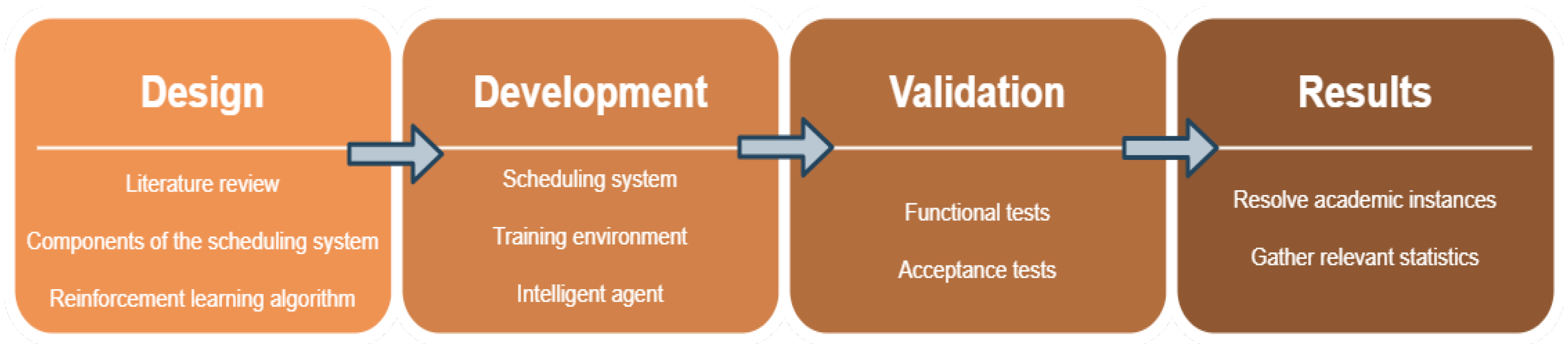
The development process of this work was divided into four main phases: design and planning of the work to be developed; the development of the system itself; comprehensive system validation; and collection of results. These phases are based on the hybrid cascade model proposed by Sommerville [51]; with it, it is possible to take advantage of the structure offered by the cascade models in conjunction with the rapid prototyping of evolutionary models [51].
A traditional cascade approach begins by defining the system requirements that shall serve as the basis for software design. In the implementation phase, each previously designed component is converted into a unit that can be tested later. In evolutionary development, an implementation of the system is made right from the start. This is then evaluated and iteratively the system is refined to a satisfactory level. This requires the specification of requirements, development and validation to occur simultaneously.
The methodology employed in this paper follows an hybrid approach as it combines the two discussed models: cascade and evolutionary. It follows, in part, the cascade model because it began with the specification of requirements that serve as the basis for the implementation of the system, then moved on to the development phase of the system. Once this phase was over, the overall system was tested and, finally, the relevant statistical results and values were collected. However, at a lower granularity level an evolutionary model [51] was applied. The initial version of each component was tested as it was developed (as if it were a prototype). Then, each version of the components was worked on in an iterative manner, enhancing the previous versions. At last, the final version was built and combined in the overall system. The development process of this work, from the initial research to the achievement and analysis of the results, is split into four phases: design, development, validation and results. These are detailed on the following paragraphs and illustrated in Figure 2.
The design phase is the initial phase of the project. Thus, it is not surprising that in it there are activities such as the revision of the state-of-the-art of the scientific areas involved, namely the reinforcement learning algorithms and the training environments of agents that use these algorithms. In the machine learning module, the design phase consisted then in the revision of the state-of-the-art mentioned, which was previously published [2]. This served as the basis for specifying the training environment of the agent to be developed and in the decision of the learning algorithm to use–proximal policy optimization (PPO) [52]. For the scheduling module this phase served to concretely define each of the components of the problems: jobs, the operations that compose each job, the machines where the operations are performed and the decoder of academic instances of these problems.
4.2. Proposed Architecture
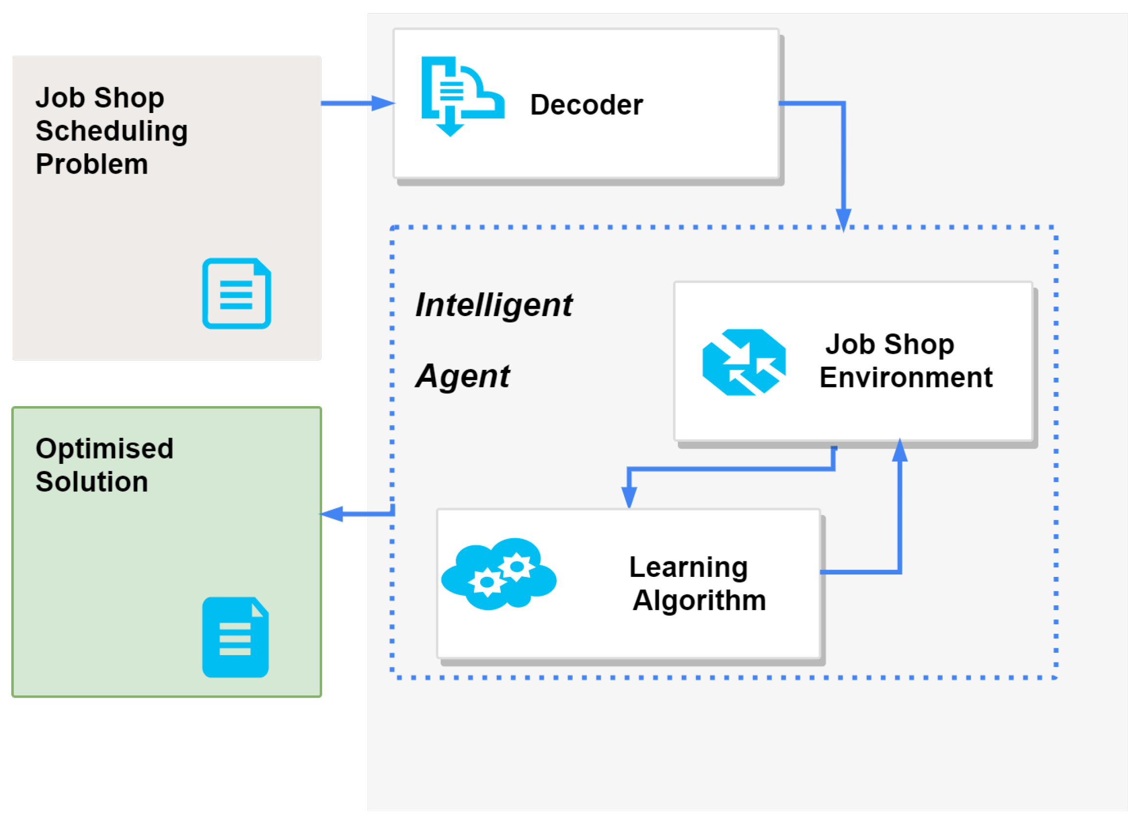
The overview of the developed system architecture is presented in Figure 3. It illustrates the division of the developed system into five different components: the JSSP instance, the problem decoder, the Job Shop environment and the learning algorithm—which, combined, constitute the intelligent agent—and, finally, the optimized solution to the problem. As a result, the system is activated by giving an instance of a JSSP to be solved. The format of the files that are used is based on the Taillard proposal [53], widely adopted by the scientific community. These files are, in practice, text files where it is known beforehand that in certain rows and columns there is specific information that determines the problem. This file is then used by the next component in the system: the decoder. It is responsible for converting the information contained in the file into workable objects in the system; that is, creating the machine, job and operation objects needed to represent all the information.
The decoder uses all this information to create the objects, which will be supplied to the intelligent agent so that it can solve the problem. A validation mechanism of the information contained in the system has also been developed to ensure that the information in the file is complete.
After all the problem information is made available to the system by the decoder, it is ready to be processed by the intelligent agent. The agent consists of two components, the training environment and the learning technique, which cooperate to obtain the solution to the problem. The Job Shop environment is where all the idiosyncrasies of this type of scheduling problem are established and verified. In practice, this is the execution and implementation of a previously proposed architecture [2].
It is in this environment that all objects processed by the decoder live. Thus, it is here that the operation objects are allocated to the machine objects according to the respective processing orders and always respecting the times defined in the instance to be solved. The approval of the allocations is made by a validation entity that has access to all the system information, designed according to software standards that are quite common in modern systems: observation, mediation, responsibility and command [54].
If the Job Shop environment is the place where the intelligent agent’s decisions are executed, it is the learning algorithm that enables the agent to know the best decision to make at any given moment. The proposed architecture employs a Deep Q-Network [55]. The two main reasons are the ability to gain experience via replays and the separate neural network to estimate the Q-value, i.e., the long-term return of the current state after taking an action based on the agent’s policy.
Considering the moment immediately after the Job Shop environment is configured with the instance provided by the decoder, all operations are available and not allocated to a machine (i.e., they do not have the start time set). The agent learning component is then responsible for deciding which operations to allocate and when. After all jobs are completely assigned and with all times defined, the agent decides whether it is better to repeat the entire assignment process based on the new knowledge acquired or, alternatively, if the current knowledge is sufficient to calculate the optimal definitive plan.
Finally, the optimized solution is the compilation of information relevant to the scheduling plan, including the final execution times. In practice, the optimized solution defines the start and end times for each operation of each job. Thus, it is possible to know where and when any job will be executed and how long it will take. Metrics that are relevant for the quality analysis, such as total makespan, are also available, so that it is easy for the end user (such as a planner or an automated factory environment) to validate its effectiveness.
5. Computational Study
This section presents the results obtained from the computational study carried out under this paper. This computational study is divided into two phases of performance analysis, both in terms of efficiency and effectiveness. In the efficiency analysis, we compare the CPU runtime of the studied approaches. In the effectiveness analysis we use the normalized makespan to measure the quality of the obtained solutions by the chosen methods. The objective is to verify the advantage of the use of reinforcement learning to solve Job Shop scheduling problems.
In the efficiency analysis, the execution times of the studied approaches are compared until a solution is obtained. In the efficiency analysis, the quality of the solutions obtained by the chosen methods of makespan minimization are evaluated. The objective is to verify the advantage of the time/quality ratio achieved by the system solutions proposed in this paper.
The JSSP solving experiments aimed at minimizing the completion time (makespan), not only because this is the most common goal dealt with in scheduling problems [2] but also because this is the goal used in the academic instances.
In the initial training phase, scheduling problem instances were provided to the agent in a random way so that he could freely train and learn how to solve the problems. Then, for each proposed solution, a reward was calculated and returned to the agent, which was used by him to improve his performance. The formula used to calculate the reward takes into account the distance of the completion time obtained to the best possible completion time for the instance used.
The resolution method consisted of providing each problem instance to the developed agent and, for each instance, storing the conclusion time obtained and the execution time from the decoding of the instance to be solved to the recording of the solution obtained. These are the components on which this computational study is based.
The implementation of the system (based on the proposed architecture Section 4.2) was done using Python because of the development speed, the ease of creating and publishing prototypes and the existing support for the programming language. It was perhaps the most likely choice, considering that Python is the most widely used programming language in projects involving work with data and/or machine learning [56,57].
The machine used during the development of this work and for the computational study has the following characteristics: A 3.30 GHz Intel Core i-5 6600 CPU, 16 GB of 2133 MHz DDR4 memory, a 1 TB Seagate Barracuda ST1000DM003 hard drive, Gigabyte GeForce GTX 1060 graphics card with 6 GB of 192-bit GDDR5 memory, plus the Windows 10 Pro operating system. Despite being a machine with a decent capacity, it is still intended for personal use, being quite distant from the high-end computers traditionally used by large laboratories and companies in machine learning computations, such as an RTX 8000 graphics card with 48 GB of ram or even TPUs, specialized boards for machine learning applications developed by Google [58]. Thus, the entire process of developing and training the intelligent agent had to be carefully measured in order to make the best use of the available resources.
By analyzing contemporary literature and the results published to date for the best solutions, it is possible to realize that, unfortunately, it is quite rare for complete results to be shared and to find a complete study that uses all the common academic problem instances. Analyzing the cases of Zhang et al. [59] or Peng et al. [60], the resolution of the standard Taillard instances [53] only includes the information obtained up to the TAI50 instance. This is most likely due to one of two reasons: either the authors did not consider these instances given that some authors classify them as the least interesting or not challenging enough [61], or they did not use them considering the exponential increase in the complexity of the problems (the number of jobs increases from 30 to 100), which could result in a less positive result. Considering this factor that is common in many publications, the presented computational study presented uses the academic instances proposed by Taillard [53]. In the execution time analysis, solutions are calculated for all instances up to number 50, in order to obtain directly comparable results. However, and despite the lack of a comparative term, the results and complete data obtained with this work for the remaining Taillard [53] instances (i.e., TAI51 to TAI80) are also presented in the analysis of the quality of solutions.
5.1. Efficiency Analysis
There is plenty of scientific literature with results obtained for these problems; unfortunately, it is very rare that those shares with the scientific community include the runtimes. There can be many reasons for this that only the authors would known. For example, if we are only concerned with obtaining the best possible result for a theoretical scenario, the runtime may not be relevant, e.g., in [62] the best result known to date is presented for the TAI11 instance, but the same runtimes are always used: either 5000 or 30,000 s, about 83 and 500 min, respectively. This means that execution times are often ignored, rather using a continuous repetition approach, with a predetermined time value being the stop condition. This approach may have advantages in the resolution of academic instances. However, it would be very complicated to put into practice in a real scenario for two main reasons: first, it would be prohibitive for any factory to wait long periods of time to know the job processing order, because it would cause a very big drop in productivity; and, also, any form of external disruption would cause the process to restart (e.g., if a new job were to arrive in the meantime it would be necessary to recalculate the whole plan). In fact, this is one of the main advantages of the approach developed in this paper. Whatever the complexity of the problem, the developed agent can solve it acceptably in a few seconds. For example, Ref. [49] presents some of the best results known to date for some problem instances, such as TAI32. However, the runtime to obtain this solution was 1000 s, approximately 16 and a half minutes. For the same problem, Ref. [59] presents an execution time of 497 s (approximately 8 min), while [60] needed 457 (7 and a half minutes). In the approach developed within this paper, the execution time is around 2 s.
As such, we want to analyze the runtime of different approaches for the 50 problems, TAI1-TAI50. The first two methods are those proposed by Zhang et al. [59] and Peng et al. [60], identified as Zhang and Peng, respectively. These were chosen since they represent two of the best available approaches to reach near-optimal solutions. The other two approaches are based on priority rules, which are common heuristics that can be used to obtain a valid solution. Based on a previous study [2], we have chosen two of the most common heuristics used in the daily life of a planner: the Longest Processing Time (identified as LPT) heuristic and the Shortest Processing Time (identified as SPT) heuristic. These make an allocation considering the available job with the shortest total processing time or, as opposed to the previous one, the job with the longest remaining processing time. At last, the results obtained by this work, based on the PPO algorithm [50], are identified by the abbreviation CUN.
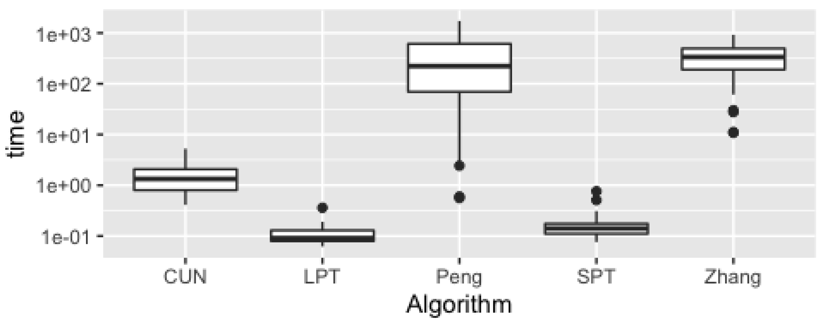
Figure 4 presents the runtime boxplot for the TAI1-TAI50 problems. Considering that the runtime for Peng and Zhang is much bigger than the runtime of other three methods we use the logarithmic axis on time axis on both graphics. From its analysis, we can see that the LPT and SPT methods are the fastest (median around 0.1 s), with CUN having a median runtime of 1.0 s. The approaches by Peng and Zhang have a much higher median runtime, and it is possible to conclude that they take significantly more time than the other methods.
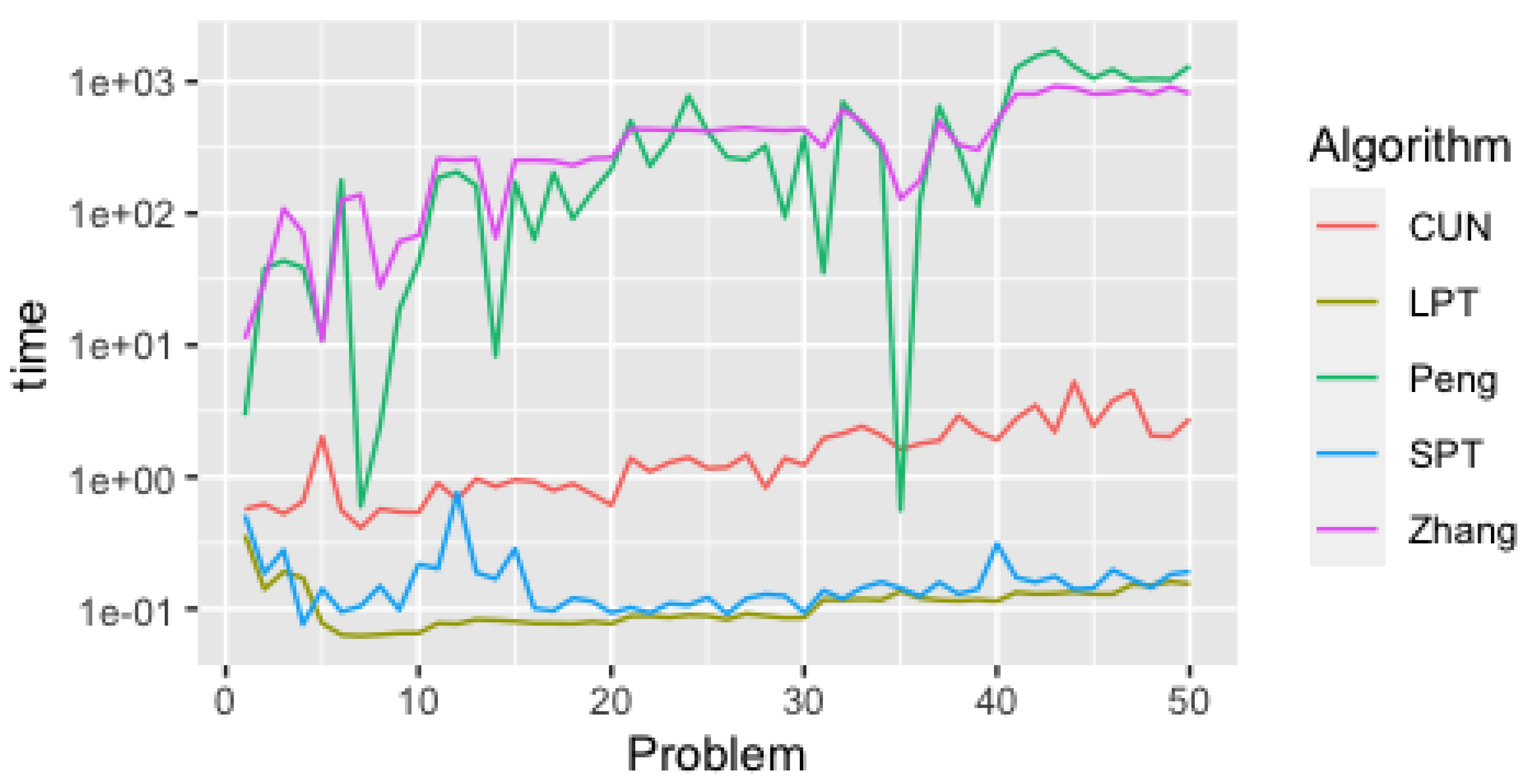
Figure 5 displays the runtime required for each method to solve each of the 50 problem instances. Similarly to Figure 4, Figure 5 also applies a logarithmic scale given the high differences between all methods. From its analysis we can see how the time required to solve each problems evolves with the increasing complexity of each instance.
In order to validate the veracity and statistical significance of the data presented here, a statistical inference analysis was conducted.
We use a Friedman test [63] to compare the 5 runtime algorithms. As expected, we got a p-value < 2 × 10⁻¹⁶ so we reject the null hypothesis and can conclude that there significant differences between the runtime algorithms considered. In order to detect pairwise runtime algorithms that have a significant difference we conduct a Nemenyi test [64] and we got the pairwise p-values shown on Table 1.
By analyzing Figure 4 and Figure 5 and Table 1, we can conclude that the two heuristic approaches (SPT and LPT) and the intelligent agent discussed in this work (CUN) improve significantly the runtime relatively to the Zhang and Peng methods.
For problems with 20 or less jobs and 15 machines (TAI01 to TAI20), the agent (CUN) takes less than 1 s to calculate a solution; Zhang and Peng take more than 4 min. Instances with 20 machines and 20 jobs (TAI21 to TAI30) take less than 1.5 s, and the other proposals are already around 7 min. This discrepancy is consistent throughout all instances, increasing the separation in execution times exponentially as the complexity of the problems grows. In fact, in terms of speed from the moment the problem reaches the system until the solution is calculated, no similar execution time has been found in contemporary literature to those presented here, except for deterministic heuristics (such as SPT and LPT) or random job allocation approaches.
We should also point out that, between CUN, SPT and LPT, CUN spends takes significantly more time to conclude, with a significance level of 5%, than the two heuristics. Although CUN is slower than SPT and LPT, we expect that the quality of CUN’s solutions will compensate this draw back. This issue is covered in the quality analysis Section 5.2.
5.2. Quality of Solutions Analysis
Based on the presented literature review (Section 2), it can be argued that the most used metric to measure the quality of a plan is its makespan, which represents the time of completion of the last operation of a plan. Thus, this section analyzes and compares the makespan of the solutions obtained by the proposed system with those obtained with SPT and LPT, for instances TAI1-TAI80.
The known optimal values [49] for each problem are included in this analysis (or best known upper bound when there is no optimal value. However, it is important to note that these makespan values for each instance have, in the great majority, different authors. As a result that there is not a common unsurpassed technique for JSSPs, customized approaches have been developed for the needs of each instance. These strategies achieve the goal of obtaining the best-known result for a given instance but, unfortunately, cannot be replicated on other instances. For example, Vilím et al. [65] present the optimal solution value for the instances TAI27 and TAI28 (among others), but the optimal solution value for the TAI29 problem was proposed by Siala et al. [66].
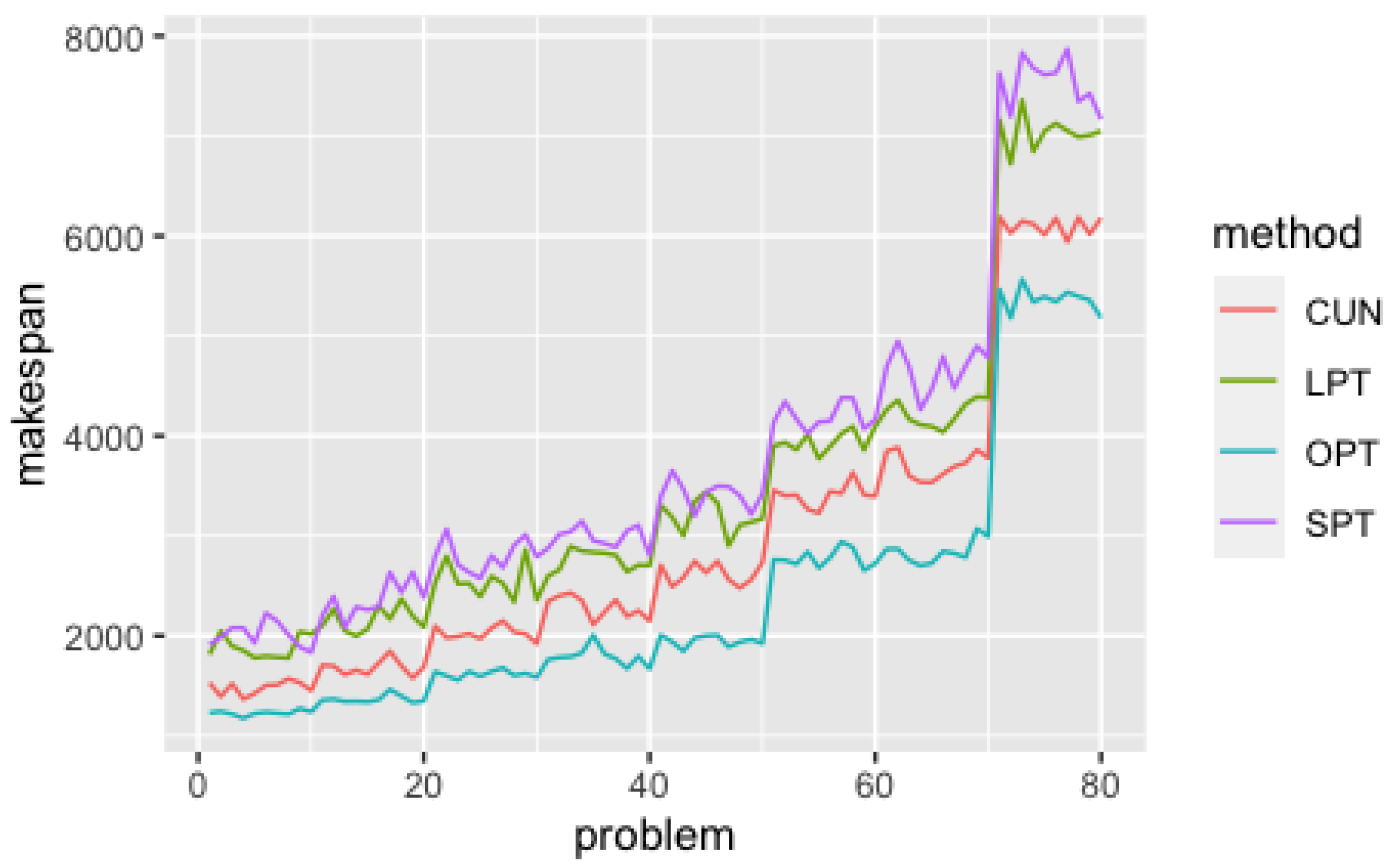
Figure 6 shows a graph containing the optimal (or best known upper bound) makespan (OPT) and the makespan obtained by each method. The OPT line (in blue) represents the known optimal value [49] (or best known upper bound) and, as such, no other method can go below it. By analyzing Figure 6, it can be verified that the SPT method is the one that needs more time to complete all problems, while CUN obtained the better solution values.
Frequently, the normalized makespan is used as a measure (instead using the raw makespan value) to compare the quality of the solutions [2]. The formula is described in Equation (3), where met represents a given method and opt represents the optimum value. Thus, the normalized makespan is the ratio between the difference of the makespan of a given method with the optimal makespan and the optimal makespan.
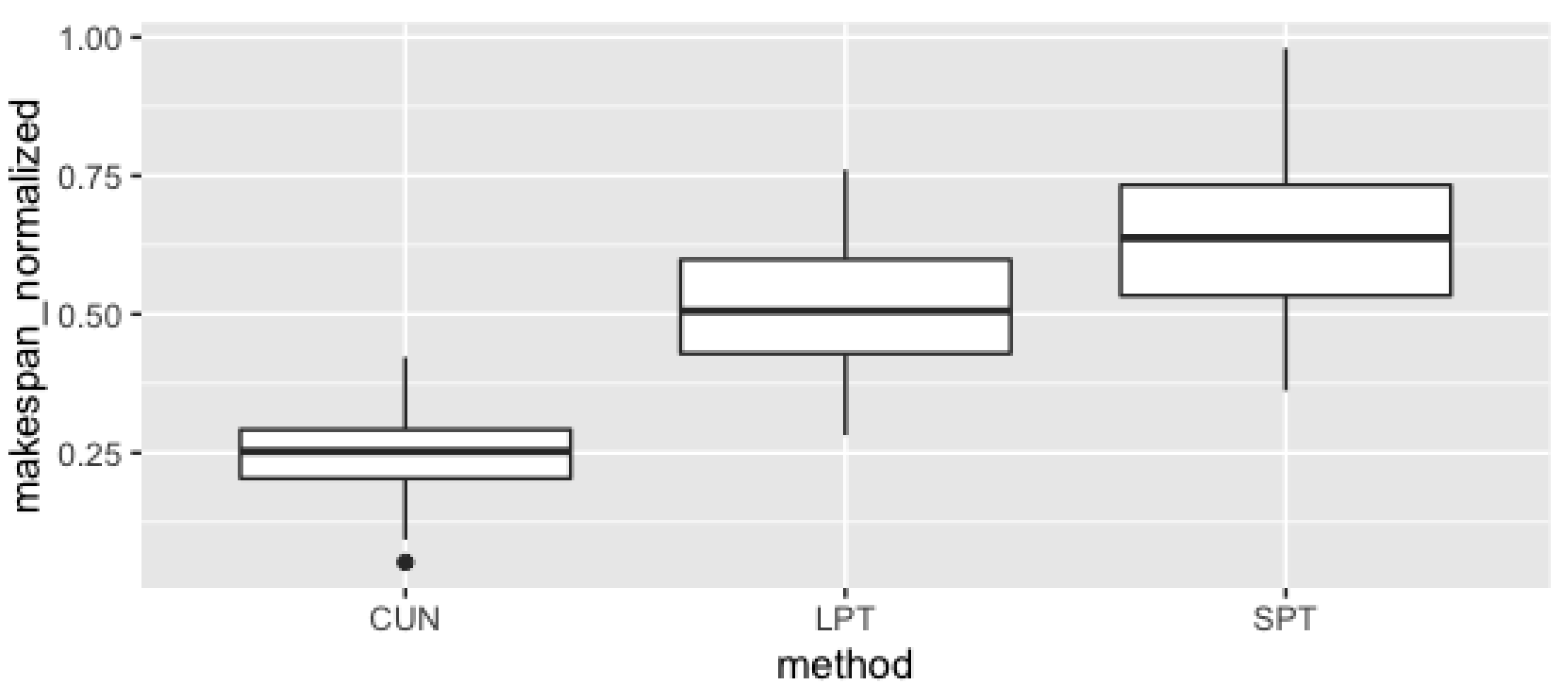
Figure 7 contains the boxplots of the normalized makespan of the three methods. The same conclusion can be reached in both measures. In fact, we can observe that for CUN the median of normalized makespan is very near to 0.25, for LPT the median is close to 0.5 and SPT has a median near of 0.6. We can conclude about evidences of the advantage in the CUN system performance when compared with LPT and SPT.
In order to validate the results obtained, a statistical inference analysis was performed. Similarly to the efficiency analysis (Section 5.1) we conducted a Friedman test [63] to detect if these differences are statistic significant.
A p-value < 2.2 × 10⁻¹⁶ was obtained from the Friedman test, which allows us to conclude that there are significant differences, in the medians, of the normalized makespan of the three methods. In order to decide which heuristics are significantly different from each other we perform, like in Section 5.1, a Nemenyi test [64] and we got the pairwise p-values shown in Table 2.
We can conclude that the differences between all pairs are significant and that the CUN results (i.e., the agent proposed in this work) represent significantly better solutions than the LPT and SPT heuristics.
5.3. Discussion of Results
When considering the impact and importance of scheduling plans in a real industry, there are two main factors that stand out: the quality of the plan and the time needed to obtain it. Thus, the results presented in this section focus on two aspects: time to solve a problem instance and the quality of the solutions obtained. It is important to emphasize that the objective of this work is not to obtain the best possible plan (unlike many metaheuristic approaches), but a plan good enough to be put into production that is obtained as soon as possible.
In terms of the quality of the solutions, two different methods were used as a term of comparison: SPT and LPT. The results discussed in this section show that the quality of the agent’s solutions is far superior to these priority rules (Figure 7).
Regarding the efficiency, it is undeniable that the work done here is efficient to find a solution to any scheduling problem presented—the runtime is limited to a few seconds on any problem. As a term of comparison, the works developed by Zhang et al. [59] and Peng et al. [60] were used. These are based on the use of efficient metaheuristics, which achieve good solutions in a timely manner. The solutions obtained by these approaches are qualitatively better (as expected); however, when compared with the results obtained in this work it becomes clear that the concept of useful time to obtain a solution is drastically changed. The results obtained by previous approaches had space for longer runtimes since the alternative would be the use of static rules, such as SPT or LPT, which present median results. With this work, this concept is completely disrupted, because it is able to obtain good plans in superbly short times. Moreover, the intelligent agent responsible for the solutions is constantly learning, so their quality is expected to improve with its use over time. We can conclude that the proposed system obtained a good compromise considering the efficiency-effectiveness binomial.
Considering the above information, it is possible to affirm that the results obtained by the proposed system (and its intelligent agent) have achieved the proposed objectives. The time it takes to obtain acceptable plans makes the use of other approaches undesirable—only in a theoretical-academic scenario is it justified to wait more than 15 min (Figure 4) for an excellent solution when one can have a very good solution in less than 2 s.
6. Conclusions
The scientific question of this paper is to investigate the benefits and usefulness of applying machine learning techniques to scheduling systems as an optimizer, with the goal of improving the overall performance of the final scheduling plans. The work presented in this paper confirms this possibility through the development of an intelligent agent. This agent takes advantage of its architecture to independently solve Job Shop problems according to its beliefs about which actions are best. The agent aims to obtain an optimized scheduling plan efficiently, thus reducing waiting times and demonstrating adaptability by being prepared to deal with unforeseen or dynamic situations (where new tasks can appear at any time). This agent achieved a very satisfactory quality, offering an alternative for calculating solutions for Job Shop scheduling problems that balances (in time) the cost of calculating solutions with the benefit of improving their quality.
By analyzing the presented results, we consider considered that the proposed objective was fulfilled. In this process, and for this to be possible, it was necessary to achieve several objectives, of which we highlight:
- Modeling the Job Shop category scheduling problem into a reinforcement learning problem by adapting the Markov process, covering how rewards are calculated, the possible set of states and the achievement of an agent’s goals or the set of available actions.
- Design and implementation of training environment for reinforcement learning algorithms to create intelligent agents capable of solving the category Job Shop scheduling problem.
- Implementation of the complete scheduling system, composed of the artificial intelligence module, which includes the intelligent agent and the training environment used during learning, and the scheduling module, which establishes all the rules of the problem, supports the decoding of academic instances and ensures the correct definition of all the components of the problem: machines, tasks and operations.
- Execution of a computational study for the analysis and validation of the results obtained by the intelligent agent developed in this work, which analyzes the performance, in efficiency and effectiveness, using measurements of the runtimes of the approaches studied and the quality of the solutions obtained, respectively.
Thus, the main contribution of this work is the conclusion (with statistical significance) about the benefits of using an intelligent agent created with reinforcement learning techniques, in a proposed novel training environment, and incorporated into a complete scheduling system that operates as the component that solves the Job Shop scheduling problems.
Author Contributions
Conceptualization, A.M., B.C.; methodology, B.C., B.F.; software, B.C.; validation, A.M. and B.F.; formal analysis, J.M.; investigation, A.M., B.C., B.F. and J.M.; resources, A.M.; data curation, B.C.; writing—original draft preparation, B.C.; writing—review and editing, A.M., B.C. and B.F.; visualization, B.C., J.M.; supervision, A.M., B.F. All authors have read and agreed to the published version of the manuscript.
Funding
This research received no external funding.
Conflicts of Interest
The authors declare no conflict of interest.
References
- Brynjolfsson, E.; Hitt, L.M. Beyond computation: Information technology, organizational transformation and business performance. J. Econ. Perspect. 2000, 14, 23–48. [Google Scholar] [CrossRef] [Green Version]
- Cunha, B.; Madureira, A.M.; Fonseca, B.; Coelho, D. Deep Reinforcement Learning as a Job Shop Scheduling Solver: A Literature Review. In Hybrid Intelligent Systems; Springer: Cham, Switzerland, 2020; pp. 350–359. [Google Scholar]
- Pinedo, M.L. Scheduling: Theory, Algorithms, and Systems, 5th ed.; Springer: Berlin Heidelberg, Germany, 2016; pp. 1–670. [Google Scholar] [CrossRef]
- Zhang, J.; Ding, G.; Zou, Y.; Qin, S.; Fu, J. Review of job shop scheduling research and its new perspectives under Industry 4.0. J. Intell. Manuf. 2019, 30, 1809–1830. [Google Scholar] [CrossRef]
- Madureira, A.; Pereira, I.; Falcão, D. Dynamic Adaptation for Scheduling Under Rush Manufacturing Orders With Case-Based Reasoning. In Proceedings of the International Conference on Algebraic and Symbolic Computation (SYMCOMP), Lisbon, Portugal, 9–10 September 2013. [Google Scholar]
- Villa, A.; Taurino, T. Event-driven production scheduling in SME. Prod. Plan. Control 2018, 29, 271–279. [Google Scholar] [CrossRef]
- Duplakova, D.; Teliskova, M.; Duplak, J.; Torok, J.; Hatala, M.; Steranka, J.; Radchenko, S. Determination of optimal production process using scheduling and simulation software. Int. J. Simul. Model. 2018, 17, 609–622. [Google Scholar] [CrossRef]
- Balog, M.; Dupláková, D.; Szilágyi, E.; Mindaš, M.; Knapcikova, L. Optimization of time structures in manufacturing management by using scheduling software Lekin. TEM J. 2016, 5, 319. [Google Scholar]
- Sun, X.; Wang, Y.; Kang, H.; Shen, Y.; Chen, Q.; Wang, D. Modified Multi-Crossover Operator NSGA-III for Solving Low Carbon Flexible Job Shop Scheduling Problem. Processes 2021, 9, 62. [Google Scholar] [CrossRef]
- Dupláková, D.; Telišková, M.; Török, J.; Paulišin, D.; Birčák, J. Application of simulation software in the production process of milled parts. SAR J. 2018, 1, 42–46. [Google Scholar]
- Madureira, A. Aplicação de Meta-Heurísticas ao Problema de Escalonamento em Ambiente Dinâmico de Produção Discreta. Ph.D. Thesis, Tese de Doutoramento, Universidade do Minho, Braga, Portugal, 2003. [Google Scholar]
- Gonzalez, T. Unit execution time shop problems. Math. Oper. Res. 1982, 7, 57–66. [Google Scholar] [CrossRef]
- Rand, G.K.; French, S. Sequencing and Scheduling: An Introduction to the Mathematics of the Job-Shop. J. Oper. Res. Soc. 1982, 13, 94–96. [Google Scholar] [CrossRef]
- Brucker, P. Job-shop scheduling problemJob-shop Scheduling Problem. In Encyclopedia of Optimization; Floudas, C.A., Pardalos, P.M., Eds.; Springer: Boston, MA, USA, 2009; pp. 1782–1788. [Google Scholar] [CrossRef]
- Beirão, N. Sistema de Apoio à Decisão para Sequenciamento de Operações em Ambientes Job Shop. Master’s Thesis, Faculdade de Engenharia da Universidade do Porto, Porto, Portugal, 1997. [Google Scholar]
- Cook, S.A. The complexity of theorem-proving procedures. In Proceedings of the third Annual ACM Symposium on Theory of Computing, Shaker Heights, OH, USA, 3–5 May 1971; pp. 151–158. [Google Scholar]
- Cormen, T.H.; Leiserson, C.E.; Rivest, R.L.; Stein, C. Introduction to Algorithms; The MIT Press: Cambridge, MA, USA, 2009. [Google Scholar]
- Yamada, T.; Yamada, T.; Nakano, R. Genetic Algorithms for Job-Shop Scheduling Problems. In Proceedings of the Modern Heuristi for Decision Support, London, UK, 18–19 March 1997; pp. 474–479. [Google Scholar]
- Madureira, A.; Cunha, B.; Pereira, J.P.; Pereira, I.; Gomes, S. An Architecture for User Modeling on Intelligent and Adaptive Scheduling Systems. In Proceedings of the Sixth World Congress on Nature and Biologically Inspired Computing (NaBIC), Porto, Portugal, 30 July–1 August 2014. [Google Scholar]
- Wang, H.; Sarker, B.R.; Li, J.; Li, J. Adaptive scheduling for assembly job shop with uncertain assembly times based on dual Q-learning. Int. J. Prod. Res. 2020, 1–17. [Google Scholar] [CrossRef]
- Ojstersek, R.; Tang, M.; Buchmeister, B. Due date optimization in multi-objective scheduling of flexible job shop production. Adv. Prod. Eng. Manag. 2020, 15. [Google Scholar] [CrossRef]
- Samuel, A.L. Some Studies in Machine Learning Using the Game of Checkers. IBM J. Res. Dev. 1959, 3, 210–229. [Google Scholar] [CrossRef]
- Mitchell, T.M. Machine Learning; McGraw-Hill, Inc.: New York, NY, USA, 1997; Volume 4, pp. 417–433. [Google Scholar] [CrossRef]
- Cascio, D.; Taormina, V.; Raso, G. Deep CNN for IIF Images Classification in Autoimmune Diagnostics. Appl. Sci. 2019, 9, 1618. [Google Scholar] [CrossRef] [Green Version]
- Cascio, D.; Taormina, V.; Raso, G. Deep Convolutional Neural Network for HEp-2 Fluorescence Intensity Classification. Appl. Sci. 2019, 9, 408. [Google Scholar] [CrossRef] [Green Version]
- Joshi, A.V. Machine Learning and Artificial Intelligence; Springer: Cham, Switzerland, 2020. [Google Scholar]
- Burkov, A. The Hundred-Page Machine Learning Book; CHaleyBooks: Muncie, IN, USA, 2019; p. 141. [Google Scholar]
- Everitt, B. Cluster analysis. Qual. Quant. 1980, 14, 75–100. [Google Scholar] [CrossRef]
- Zimek, A.; Schubert, E. Outlier Detection. In Encyclopedia of Database Systems; Springe: New York, NY, USA, 2017; pp. 1–5. [Google Scholar] [CrossRef]
- Roweis, S.T.; Saul, L.K. Nonlinear dimensionality reduction by locally linear embedding. Science 2000, 290, 2323–2326. [Google Scholar] [CrossRef] [PubMed] [Green Version]
- Scudder, H. Probability of error of some adaptive pattern-recognition machines. IEEE Trans. Inf. Theory 1965, 11, 363–371. [Google Scholar] [CrossRef]
- McClosky, D.; Charniak, E.; Johnson, M. Effective self-training for parsing. In Proceedings of the HLT-NAACL 2006—Human Language Technology Conference of the North American Chapter of the Association of Computational Linguistics, New York, NY, USA, 4–9 June 2006. [Google Scholar] [CrossRef]
- Yarowsky, D. Unsupervised word sense disambiguation rivaling supervised methods. In Proceedings of the 33rd Annual Meeting of the Association for Computational Linguistics, Cambridge, MA, USA, 26–30 June 1995; pp. 189–196. [Google Scholar] [CrossRef] [Green Version]
- Blum, A.; Mitchell, T. Combining labeled and unlabeled data with co-training. In Proceedings of the Annual ACM Conference on Computational Learning Theory, Madison, WI, USA, 24–26 July 1998. [Google Scholar] [CrossRef]
- Zhou, Z.H.; Li, M. Tri-training: Exploiting unlabeled data using three classifiers. IEEE Trans. Knowl. Data Eng. 2005, 17, 1529–1541. [Google Scholar] [CrossRef] [Green Version]
- Sutton, R.S.; Barto, A.G. Reinforcement Learning: An Introduction, 2nd ed.; The MIT Press: Cambridge, MA, USA, 2018. [Google Scholar]
- Thorndike, E.L. The Law of Effect. Am. J. Psychol. 1927, 39, 212–222. [Google Scholar] [CrossRef]
- Silver, D.; Huang, A.; Maddison, C.J.; Guez, A.; Sifre, L.; van den Driessche, G.; Schrittwieser, J.; Antonoglou, I.; Panneershelvam, V.; Lanctot, M.; et al. Mastering the game of Go with deep neural networks and tree search. Nature 2016, 529, 484–489. [Google Scholar] [CrossRef]
- Silver, D.; Schrittwieser, J.; Simonyan, K.; Antonoglou, I.; Huang, A.; Guez, A.; Hubert, T.; Baker, L.; Lai, M.; Bolton, A.; et al. Mastering the game of Go without human knowledge. Nature 2017, 550, 354–359. [Google Scholar] [CrossRef]
- Akkaya, I.; Andrychowicz, M.; Chociej, M.; Litwin, M.; McGrew, B.; Petron, A.; Paino, A.; Plappert, M.; Powell, G.; Ribas, R.; et al. Solving Rubik’s Cube with a Robot Hand. arXiv 2019, arXiv:1910.07113. [Google Scholar]
- Nagabandi, A.; Konoglie, K.; Levine, S.; Kumar, V. Deep Dynamics Models for Learning Dexterous Manipulation. arXiv 2019, arXiv:1909.11652. [Google Scholar]
- Wu, J.; Wei, Z.; Liu, K.; Quan, Z.; Li, Y. Battery-Involved Energy Management for Hybrid Electric Bus Based on Expert-Assistance Deep Deterministic Policy Gradient Algorithm. IEEE Trans. Veh. Technol. 2020, 69, 12786–12796. [Google Scholar] [CrossRef]
- Wu, J.; Wei, Z.; Li, W.; Wang, Y.; Li, Y.; Sauer, D.U. Battery Thermal- and Health-Constrained Energy Management for Hybrid Electric Bus Based on Soft Actor-Critic DRL Algorithm. IEEE Trans. Ind. Inform. 2021, 17, 3751–3761. [Google Scholar] [CrossRef]
- Kaplan, R.; Sauer, C.; Sosa, A. Beating Atari with Natural Language Guided Reinforcement Learning. arXiv 2017, arXiv:1704.05539. [Google Scholar]
- Salimans, T.; Chen, R. Learning Montezuma’s Revenge from a Single Demonstration. arXiv 2018, arXiv:1812.03381. [Google Scholar]
- Schulman, J.; Levine, S.; Abbeel, P.; Jordan, M.; Moritz, P. Trust region policy optimization. In Proceedings of the 32nd International Conference on Machine Learning (ICML-15), Lille, France, 6–11 July 2015; pp. 1889–1897. [Google Scholar]
- Sutton, R.S. Reinforcement Learning: Past, Present and Future. In Simulated Evolution and Learning; McKay, B., Yao, X., Newton, C.S., Kim, J.H., Furuhashi, T., Eds.; Springer: Berlin/Heidelberg, Germany, 1999; pp. 195–197. [Google Scholar]
- Zhang, T.; Xie, S.; Rose, O. Real-time job shop scheduling based on simulation and Markov decision processes. In Proceedings of the Winter Simulation Conference, Las Vegas, NV, USA, 3–6 December 2017; pp. 3899–3907. [Google Scholar] [CrossRef]
- van Hoorn, J.J. The Current state of bounds on benchmark instances of the job-shop scheduling problem. J. Sched. 2018, 21, 127–128. [Google Scholar] [CrossRef]
- Cunha, B.; Madureira, A.; Fonseca, B. Reinforcement Learning Environment for Job Shop Scheduling Problems. Int. J. Comput. Inf. Syst. Ind. Mana. Appl. 2020, 12, 231–238. [Google Scholar]
- Sommerville, I. Software Engineering, 9th ed.; Addison Wesley: Boston, MA, USA, 2011; ISBN 0137035152. [Google Scholar]
- Schulman, J.; Wolski, F.; Dhariwal, P.; Radford, A.; Klimov, O. Proximal policy optimization algorithms. arXiv 2017, arXiv:1707.06347. [Google Scholar]
- Taillard, E. Benchmarks for basic scheduling problems. Eur. J. Oper. Res. 1993, 64, 278–285. [Google Scholar] [CrossRef]
- Gamma, E.; Helm, R.; Johnson, R.; Vlissides, J. Design Patterns: Elements of Reusable Software; Addison-Wesley Professional Computing Series; Pearson Education: London, UK, 1996. [Google Scholar] [CrossRef]
- Mnih, V.; Kavukcuoglu, K.; Silver, D.; Graves, A.; Antonoglou, I.; Wierstra, D.; Riedmiller, M. Playing Atari with Deep Reinforcement Learning. arXiv 2013, arXiv:1312.5602. [Google Scholar]
- Pedregosa, F.; Varoquaux, G.; Gramfort, A.; Michel, V.; Thirion, B.; Grisel, O.; Blondel, M.; Prettenhofer, P.; Weiss, R.; Dubourg, V.; et al. Scikit-learn: Machine learning in Python. J. Mach. Learn. Res. 2011, 12, 2825–2830. [Google Scholar]
- Raschka, S.; Mirjalili, V. Python Machine Learning: Machine Learning and Deep Learning with Python, Scikit-learn, and TensorFlow 2; Packt Publishing Ltd.: Birmingham, UK, 2019. [Google Scholar]
- Jouppi, N. Google supercharges machine learning tasks with TPU custom chip. Google Blog May 2016, 18, 1. [Google Scholar]
- Zhang, C.Y.; Li, P.; Rao, Y.; Guan, Z. A Very Fast TS/SA Algorithm for the Job Shop Scheduling Problem. Comput. Oper. Res. 2008, 35, 282–294. [Google Scholar] [CrossRef]
- Peng, B.; Lü, Z.; Cheng, T.C.E. A tabu search/path relinking algorithm to solve the job shop scheduling problem. Comput. Oper. Res. 2015, 53, 154–164. [Google Scholar] [CrossRef] [Green Version]
- paul Watson, J.; Howe, A.E.; Whitley, L.D. Deconstructing Nowicki and Smutnicki’s i-TSAB Tabu Search Algorithm for the Job-Shop Scheduling Problem. Comput. Oper. Res. 2005, 33, 2623–2644. [Google Scholar] [CrossRef]
- Pardalos, P.M.; Shylo, O.V. An Algorithm for the Job Shop Scheduling Problem based on Global Equilibrium Search Techniques. Comput. Manag. Sci. 2006, 3, 331–348. [Google Scholar] [CrossRef]
- Friedman, M. A comparison of alternative tests of significance for the problem of m rankings. Ann. Math. Stat. 1940, 11, 86–92. [Google Scholar] [CrossRef]
- Nemenyi, P. Distribution-Free Multiple Comparisons. Ph.D. Thesis, Princeton University, Princeton, NJ, USA, 1963. [Google Scholar]
- Vilím, P.; Laborie, P.; Shaw, P. Failure-Directed Search for Constraint-Based Scheduling. In International Conference on AI and OR Techniques in Constriant Programming for Combinatorial Optimization Problems; Springer: Barcelona, Spain, 2015; pp. 437–453. [Google Scholar]
- Siala, M.; Artigues, C.; Hebrard, E. Two Clause Learning Approaches for Disjunctive Scheduling. In Principles and Practice of Constraint Programming; Pesant, G., Ed.; Springer: Cham, Switzerland, 2015; pp. 393–402. [Google Scholar]
Figure 1.
Representation of a Job Shop scheduling problem (based on Beirão proposal [15]).
Figure 1.
Representation of a Job Shop scheduling problem (based on Beirão proposal [15]).

Figure 2.
Diagram illustrating the principal activities of each phase.

Figure 3.
Diagram of the developed system (adapted from our previous proposal [50]).
Figure 3.
Diagram of the developed system (adapted from our previous proposal [50]).

Figure 4.
Boxplot of the runtime, in seconds (scientific notation), of algorithms: LPT, SPT, CUN, Peng and Zhang.
Figure 4.
Boxplot of the runtime, in seconds (scientific notation), of algorithms: LPT, SPT, CUN, Peng and Zhang.

Figure 5.
Runtime, in seconds (scientific notation), for each problem (TAI1-TAI50).

Figure 6.
Makespan for LPT, SPT, CUN and the optimal value for each instance.

Figure 7.
Boxplot of the normalized makespan of the three methods.


Table 1.
Pairwise p-values of Nemenyi [64] test for CPU runtime.
Table 1.
Pairwise p-values of Nemenyi [64] test for CPU runtime.
| Zhang | Peng | CUN | SPT | |
|---|---|---|---|---|
| Peng | - | - | - | |
| CUN | - | - | ||
| SPT | - | |||
| LPT | < |
Table 2.
Pairwise of Nemenyi [64] test for the normalized makespan values.
Table 2.
Pairwise of Nemenyi [64] test for the normalized makespan values.
| CUN | LPT | |
|---|---|---|
| LPT | - | |
| SPT | < |
Short Biography of Authors
 | Bruno Cunha is a professor at the Institute of Engineering–Polytechnic of Porto (ISEP/P.PORTO) and a researcher of the Interdisciplinary Studies Research Center (ISRC). He received his degree in informatics engineering in 2013 and master’s degree of computer science in knowledge-based and decision support technologies in 2015 from the Institute of Engineering–Polytechnic of Porto (ISEP/P.PORTO), and the PhD degree in informatics, in 2021, from the University of Trás-os-Montes and Alto Douro (UTAD). His research interests involve machine learning, optimization algorithms and computational intelligence. |
 | Ana Madureira was born in Mozambique, in 1969. She got his BSc degree in Computer Engineering in 1993 from ISEP, Master degree in Electrical and Computers Engineering–Industrial Informatics, in 1996, from FEUP, and the PhD degree in Production and Systems, in 2003, from University of Minho, Portugal. She became IEEE Senior Member in 2010. She had been Chair of IEEE Portugal Section (2015–2017), Vice-chair of IEEE Portugal Section (2011–2014) and Chair/Vice-Chair of IEEE-CIS Portuguese chapter. She was Chair of University Department of IEEE R8 Educational Activities Sub-Committee (2017–2018). She is IEEE R8 Secretary (2019–2021). She is External Member Evaluation Committee of the Agency for Assessment and Accreditation of Higher Education—A3ES for the scientific area of Informatics of Polytechnic Higher Education (since 2012). Currently she is Coordinator Professor at the Institute of Engineering–Polytechnic of Porto (ISEP/P.PORTO) and Director of the Interdisciplinary Studies Research Center (ISRC). In the last few years, she was author of more than 100 scientific papers in scientific conference proceedings, journals and books. |
 | Benjamim Fonseca is an Associate Professor with Habilitation at the University of Trás-os-Montes and Alto Douro (UTAD) and researcher at INESC TEC, in Portugal. His main research and development interests are collaborative systems, mobile accessibility and immersive systems. He authored or co-authored over a hundred publications in these fields, in several international journals, books and conference proceedings, and participates in the review and organization of various scientific publications and events. He is also co-founder and CEO of 4ALL Software, UTAD’s spin-off that works in the development of innovative software, implementing complex digital platforms and interactive solutions. |
 | João Matos is an Associate Professor at ISEP and researcher at LEMA in Porto, Portugal. He got his BSc degree in Applied Mathematics in 2005 from University of Porto, and the PhD degree in Applied Mathematics in 2015 from University of Porto. His main research interests are approximation theory, orthogonal polynomials, spectral methods and image processing. |
Publisher’s Note: MDPI stays neutral with regard to jurisdictional claims in published maps and institutional affiliations. |
© 2021 by the authors. Licensee MDPI, Basel, Switzerland. This article is an open access article distributed under the terms and conditions of the Creative Commons Attribution (CC BY) license (https://creativecommons.org/licenses/by/4.0/).
Share and Cite
MDPI and ACS Style
Cunha, B.; Madureira, A.; Fonseca, B.; Matos, J. Intelligent Scheduling with Reinforcement Learning. Appl. Sci. 2021, 11, 3710. https://0-doi-org.brum.beds.ac.uk/10.3390/app11083710
AMA Style
Cunha B, Madureira A, Fonseca B, Matos J. Intelligent Scheduling with Reinforcement Learning. Applied Sciences. 2021; 11(8):3710. https://0-doi-org.brum.beds.ac.uk/10.3390/app11083710
Chicago/Turabian StyleCunha, Bruno, Ana Madureira, Benjamim Fonseca, and João Matos. 2021. "Intelligent Scheduling with Reinforcement Learning" Applied Sciences 11, no. 8: 3710. https://0-doi-org.brum.beds.ac.uk/10.3390/app11083710
Note that from the first issue of 2016, this journal uses article numbers instead of page numbers. See further details here.