Article

Characterization of Geometry and Surface Texture of AlSi10Mg Laser Powder Bed Fusion Channels Using X-ray Computed Tomography

by
Christopher G. Klingaa
1,*,
Filippo Zanini
2,
Sankhya Mohanty
1,
Simone Carmignato
2 and
Jesper H. Hattel
1
1
Department of Mechanical Engineering, Technical University of Denmark, Produktionstorvet, Building 425, 2800 Lyngby, Denmark
2
Department of Management and Engineering, University of Padova, Stradella San Nicola 3, 36100 Vicenza, Italy
*
Author to whom correspondence should be addressed.
Submission received: 27 April 2021 / Revised: 5 May 2021 / Accepted: 7 May 2021 / Published: 10 May 2021
(This article belongs to the Topic Additive Manufacturing)

Abstract

:
Channels manufactured by laser powder bed fusion have an inherent process-induced dross formation and surface texture that require proper characterization for design and process optimization. This work undertakes surface texture characterization of AlSi10Mg channels of nominal diameter sizes ranging from 1 mm to 9 mm using X-ray computed tomography. Profile parameters, including Pa, Pz, and Pq, were found to be interchangeable for qualitative characterization of surface texture variation. Psk, Pvv, and the fractal dimension could identify the presence of extreme dross and sintered particles on the measured profiles. A method for predicting the equivalent diameter of the unobstructed cross-sectional area (Deq) was presented and its reduction was found to follow a logarithmic trend, as a function of channel length. An empirical model Pa (β, D), as a function of local angular position (β) and channel diameter (D), was demonstrated on a perfect channel geometry, resulting in well-predicted roughness and internal geometry.

1. Introduction

Channels fabricated by laser powder bed fusion (LPBF) are a promising application of metal additive manufacturing (MAM) due to the freedom of design. With the freeform nature offered by LPBF, cooling applications may be optimized using conformal cooling channel designs [1]. However, components with LPBF-manufactured overhangs and channels have been shown to have a high degree of material dross formation [2,3] which influences both the actual diameter of the channels and the surface texture [4]. During the LPBF manufacturing process, material dross forms at overhanging areas due to a local accumulation of heat arising out of the lower heat conductivity of the surrounding powder as compared to the already solidified material. With an increase in the local temperature, powder particles are typically sintered to the overhanging sections [2,5]. Some mitigation techniques include the use of teardrop-shaped channels as well as producing channels in a vertical orientation [4]. However, the nature of conformal channels does not allow for the application of these techniques at all times.
For cooling applications, the description of roughness in pipes and channels has historically been done with the equivalent sand grain roughness (ks). The detailed relation between ks, the Reynolds number i.e., the flow conditions, and the friction factor was published by Moody in the 1940s [6] and is still in use today. Friction factors and sudden diameter reductions are among the main influencing factors in the loss of pressure head and energy [7,8]. Much work has been conducted in the efforts of connecting the equivalent sand grain roughness with the more well-defined profile surface texture parameters according to ISO 4287:1997 [9]. Classic parameters such as Ra, Rz, and Rq have all been sought to be correlated with ks. In 1966, Forster [10] showed how the relation is highly dependent on the manufacturing origin of the investigated surface, reporting ks ≈ 2·Ra for machined surfaces and ks ≈ 7·Ra for emery papers. Bunker [11] found that ks ≈ 10·Ra for polished surfaces and Hummel et al. [12] observed that ks ≈ 5.2·Ra when considering various surfaces with different roughness. While the last relation may be the most appropriate for LPBF applications due to the anisotropy and randomness of the surfaces that are often observed, the large disparity in the suggested relations indicates that no congruent answer has been found [13].
The profile surface texture parameters mentioned above were developed to characterize the surface of conventional manufacturing techniques such as subtractive processes including milling and turning. With the increased interest in additive manufacturing (AM) and the rising use of the LPBF process as an addition to existing manufacturing practices, there exists a debate on whether the conventional profile and areal surface texture parameters are appropriate for adequately characterizing additively manufactured surfaces. The surface of LPBF components is typically showing complex features (including re-entrant features [14]) and a randomized surface texture, except for scanning lines being visible in some cases. Some research is focused on the development of better and more accurate frameworks and methods to determine the surface texture of additively manufactured components, including the development of new surface texture parameters [15,16,17]. In recent times, these are often used in the investigation of the influence of LPBF process parameters on the resulting surface texture [5,18]. As long as this is the case, it is important to understand the applicability of classic surface texture parameters and how they may be, or may not be, used to characterize AM surfaces.
Classic techniques for surface texture analysis are not easily used for the evaluation of internal roughness [19]. While optical techniques are increasingly used, in order to use the techniques, artifacts are typically cut into several sections. The destructive approach may limit the degree to which full characterization can be obtained. Furthermore, optical techniques have limitations in their ability to detect steep slopes, which are often present in LPBF channels [20].
The combination of X-ray computed tomography (CT) and areal surface texture parameters, according to ISO 25178-2:2012 [21], are increasingly used to characterize internal AM surfaces [15,22,23]. Areal surface texture characterization is often adequate for general characterization but may lack the ability of functional characterization for some application-specific purposes such as fluid flow, where the flow typically goes in one direction. Using X-ray CT, work has been conducted displaying how roughness varied randomly along the length of LPBF channels [24]. Other work utilizes the ability of X-ray CT to capture undercuts on a surface. This ability is unique for X-ray CT and the applicability of classic roughness parameters in the setting of including re-entrant features has been explored in the literature [25].
Additionally, an advantage of X-ray CT over conventional profilometer measurements is the abundance of data, allowing for a full characterization of the surface. A detailed characterization may be used to generate more accurate prediction models for surface texture. Such prediction models have been shown useful in the generation of predicted geometries of conformal cooling channel designs [26]. As new methods for manufacturing plastic injection molds with conformal cooling channels emerge, such as hybrid processes combining machining and laser powder bed fusion [27], adequate characterization techniques become crucial for quality inspection. X-ray CT inspection may be used for this purpose, once a proper understanding of the usage has been achieved.
This work seeks to qualitatively and quantitatively characterize aluminum LPBF channels. The characterization includes the dross and surface texture together with the actual channel diameter. The nominal channel diameters were Dnom = 1 mm, 2 mm, 3 mm, 6 mm, and 9 mm, covering a range typically used for cooling applications in tools and molds. The goal of this work is to improve upon the understanding of the appropriate use of profile parameters and the connection between the calculated parameters and the formation of dross and roughness in LPBF aluminum channels. In this work, profile parameters are used, with profiles parallel to the flow direction of the channels, because it is the texture along the flow direction that is relevant towards influencing flow dynamics. It is also the intention to shed light on the possible size effects of LPBF aluminum channels and provide simple methodologies for generating prediction models for roughness and channel diameters. Section 2 presents the investigated channel artifacts together with the chosen characterization approach. Furthermore, the section includes a proposal of a novel methodology for predicting the equivalent diameter of LPBF channels as a function of channel length. Section 3 presents the obtained results together with a discussion of the shown observations, revealing both redundancy and unique characterization properties among the calculated profile parameters. Finally, Section 4 presents the conclusions of this work.

2. Materials and Methods

In this work, LPBF-manufactured aluminum channels are characterized using X-ray computed tomography (CT) and image analysis. This section describes the investigated samples, the X-ray CT measurements, and the method to compute the considered surface texture parameters. Additionally, a description is given of the generation of a simple roughness prediction model and how it can be used to modify the initial CAD design of a channel to include the effects of dross formation on the geometry. Finally, a description of a new methodology for estimating the equivalent diameter of the unobstructed cross-sectional area is presented.

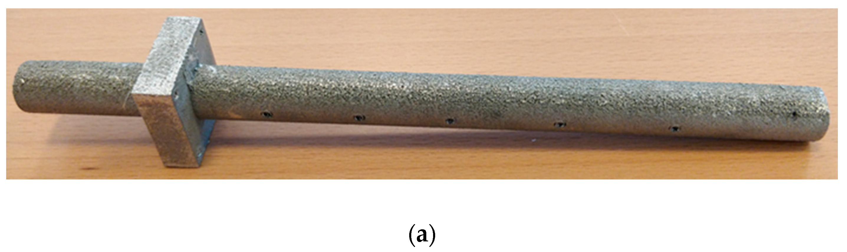
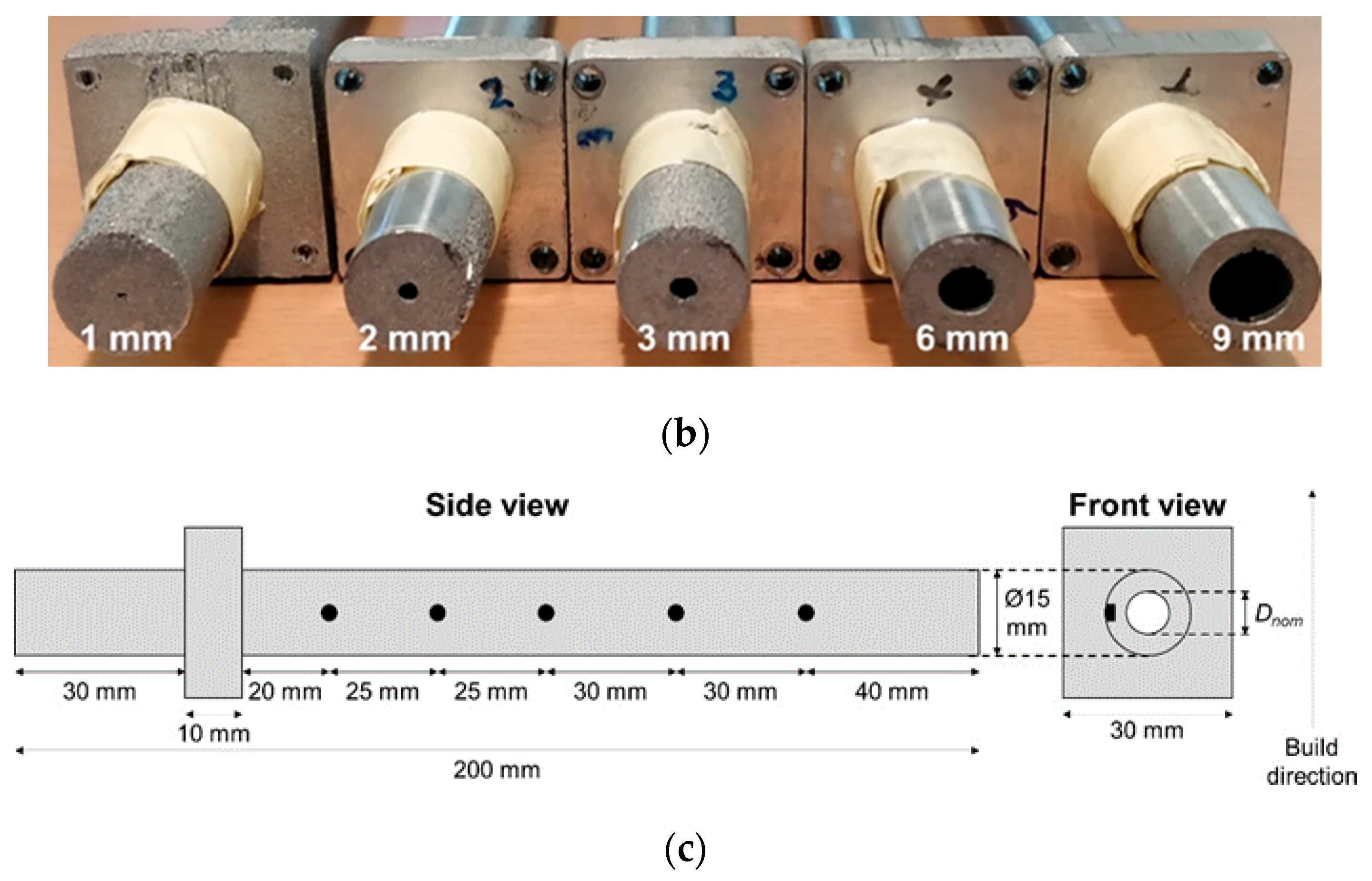
2.1. Investigated Samples

Nine LPBF aluminum channels, specifically designed to conduct cooling experiments and characterize the internal geometry and surface texture, were investigated in this work. Figure 1a shows the entirety of one of the investigated channels, while Figure 1b shows the end-view of the investigated channels with different diameters. Figure 1c illustrates a schematic overview of the dimensions of the channels. All external dimensions were kept constant, with the only varying dimension being the internal circular channel diameter Dnom. The channel diameters were Dnom = 1 mm, 2 mm, 3 mm, 6 mm, and 9 mm of which five channels with Dnom = 6 mm with suffixes A, B, C, D, and E were investigated. All channels were manufactured on an SLM 280 system in the aluminum alloy AlSi10Mg using standard settings and employing a stripe scan strategy. The used volume hatch process parameters are shown in Table 1. The channels were not post-processed after LPBF manufacture apart from the removal from the baseplate.

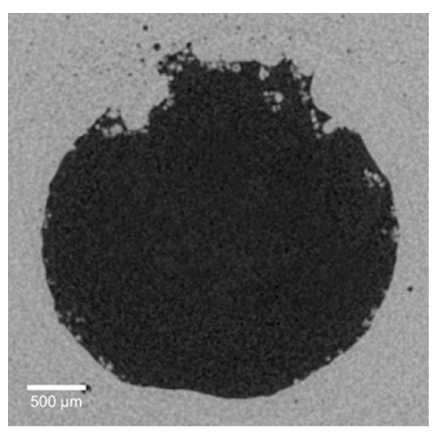
2.2. X-ray CT and Image Analysis

The X-ray CT scans were conducted using a metrological CT system (Nikon Metrology MCT225), with a micro-focus X-ray source having a minimum achievable focal spot size of 3 µm, a 16-bit X-ray detector with a 2000 × 2000 grid of 0.2 mm squared pixels, a controlled cabinet temperature (20 ± 0.5 °C), and a maximum permissible error (MPE) for length measurements equal to (9 + L/50) μm (where L is the length in mm). Each channel was scanned once, except for the channel 6 mm A, which was scanned five times for repeatability and reproducibility analysis. The scanning parameters used to acquire X-ray bi-dimensional projections were kept fixed for all scans for a better comparison of results. A total of 3141 projections were acquired with an exposure time equal to 1.415 s per projection and using a 0.1 mm Cu filter, a voltage of 200 kV, and a power of 8 W. The reconstruction of 3D models starting from the acquired projections was conducted with the CT Pro 3D software version 3.1.9 (Nikon Metrology Inc., Düsseldorf, Deutschland), which implements the filtered-back projection algorithm [28]. A beam hardening correction was applied across all scans using the preset index 2 which utilizes a second-order polynomial of the form:
y = 0.75 x + 0.25 x 2
where x is the initial gray value and y is the corrected gray value. In addition, a noise median filter with a 3 × 3 kernel size was applied to all the acquired X-ray projections before reconstruction. The obtained voxel size was equal to 9 µm.
The scanned region, with a height approximately equal to 18 mm, was the same for each of the nine channels. To do this, the third thermocouple hole from the left (Figure 1b) was positioned in the middle of the scan. The reconstructed volumes were individually realigned and cropped using the analysis and visualization software VGSTUDIO MAX 3.2 (Volume Graphics, Heidelberg, Germany). The volumes were cropped so that a total channel length of 9 mm was represented equally on either side of the thermocouple hole. The cropped volume was subsequently exported as a stack of cross-sectional TIFF images along the length of the channel, with step width equal to 9 µm. Each image from the exported stack represented a cross-sectional view of the channel as the one shown in Figure 2. For each of the nine reconstructed volumes, a stack consisting of 2000 images was generated, of which the middle 500, representing a channel length of 4.5 mm, were used for analysis. The 500 slices were selected as the default stack size for the general investigations as they could be analyzed within an acceptable computation time.

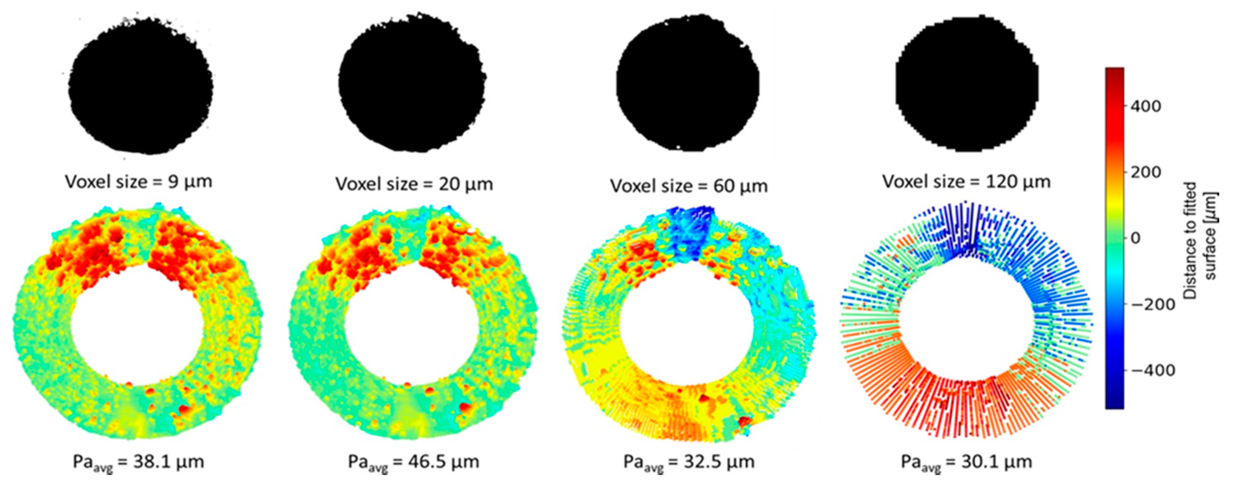
Selection of Voxel Size

A preliminary study was conducted to investigate the effect of the voxel size on the qualitative and quantitative estimations. The motivation was to determine whether larger voxel sizes could safely be used which would result in larger lengths of the channels being investigated. Figure 3 shows the analysis of the same section of the channel Dnom = 6 mm A, conducted with voxel sizes of 9 µm, 20 µm, 60 µm, and 120 µm. To fit the external diameter of the entire sample (i.e., 15 mm) within the detector field of view, leaving sufficient lateral space for acquiring information on the background grey values, voxel sizes below 9 µm were not taken into account. It must be noted that no bandwidth matching was conducting for the quantitative comparison of average Pa-values in this section.
Firstly, the quality of the cross-sectional views is greatly diminishing with the increasing voxel size. Secondly, the qualitative surface deviation maps indicate that a larger voxel size could be used in situations where only the significant surface texture patterns are of interest. The qualitative difference between a voxel size of 9 µm and 20 µm is only observable in how the smallest particles and agglomerations are not captured at a voxel size of 20 µm. This difference means little for the qualitative evaluation and overall surface texture pattern but influences the quantitative evaluation. In this case, a difference of approximately 20% is found between the estimations of the average Pa-values of the channel (see Section 2.3 for the definition of Pa). The larger average Pa-value is due to the profile extraction methodology, wherein the profiles are generated similar to a stylus being dragged across the surface. The same “probe size” was used for extracting the profiles. Having a larger voxel size and lower resolution leads to each profile representing a “broader” area of the surface. Therefore, a larger percentage of the extracted profiles will have larger deviation values, resulting in an overestimation of the average Pa-value. The broadening effect is compensated by the “smoothening” of the surface texture that occurs when the voxel size is increased further. This can be seen for the 60 µm and 120 µm cases in Figure 3, which follow the general trend of voxel size effects on areal surface texture parameters [14]. The large negative deviation observed on the top part of the 60 µm case is associated with how the nominal element is created by locally fitting an ellipse to each of the image slices used to create the 3D point cloud. The surrounding peaks of dross on both sides of the blue area in the 60 µm case have a significant influence on the fit. Therefore, the general shape deviation from the nominal geometry is being captured, resulting in negative values at the top. This tendency is even more apparent for the 120 µm case where, primarily, only the shape deviation from the nominal geometry is being captured.
Since the purpose of this work was to investigate the characterization possibilities of using different surface texture parameters, it was decided to use a voxel size of 9 µm to ensure a high enough resolution at the cost of the investigated channel length.

2.3. Definition of Surface Profile Parameters of Interest and Fractal Dimension

The surface topography characterization inside channels performed in this study was based on the methodology proposed by Klingaa et al. [29], which uses 3D point cloud data generated from 3D voxel-based data to extract surface profiles along the length of channels and at 360° around the channel periphery. The surface profiles are obtained similar to running a contact stylus across the surface of the channel. For a detailed description of the profile extraction methodology and subsequent profile preparation and analysis, the reader is referred to the aforementioned work.
The in-house Python code used in the former work was expanded in terms of the computed surface profile parameters.
In particular, the 12 calculated parameters are briefly described below. All the parameters (i.e., P-parameters) were computed on the primary profiles, obtained after removing the form error (e.g., mean line) of the original profiles. The height at a given point along the profile length x is described as Z ( x ) and the sampling length in this work was equivalent to the profile length l .
Amplitude surface profile parameters
  • Pa is the arithmetical mean deviation of the assessed profile [9]:
    P a = 1 l 0 l | Z ( x ) | d x
  • Pq is the root mean square deviation of the profile, representing the variation of the profile [9]:
    P q = 1 l 0 l Z ( x ) 2 d x
  • Pp is the maximum profile peak height [9]:
    P p = max ( Z ( x ) )
  • Pz is the maximum height of a profile [9]:
    P z = max ( Z ( x ) ) min ( Z ( x ) )
  • P10z is the average of the 10 largest heights of a profile [30]:
    P 10 z = a v g ( m a x 10 ( Z ( x ) ) m i n 10 ( Z ( x ) ) )
  • Psk is the skewness of the profile, representing mass distribution around the mean line or bias of the profile [9]:
    P s k = 1 P q 3 ( 1 l 0 l Z ( x ) 3 d x )
  • Pku is the kurtosis of the profile, representing the spikiness of the profile [9]:
    P k u = 1 P q 4 ( 1 l 0 l Z ( x ) 4 d x )
Functional parameters
Profile versions of the void and material volume parameters according to ISO 25178-2:2012 [21] and similar to the linear material ratio curve parameters [31] were implemented. The void and material volume parameters defined in ISO 25178-2:2012 [21] are typically used to analyze the fluid flow over a surface, wear potential of the surface, lubrication properties, and debris entrapment [32]. In this work, such parameters are computed using the linear material ratio curve (see Figure 4) generated from the surface profiles.
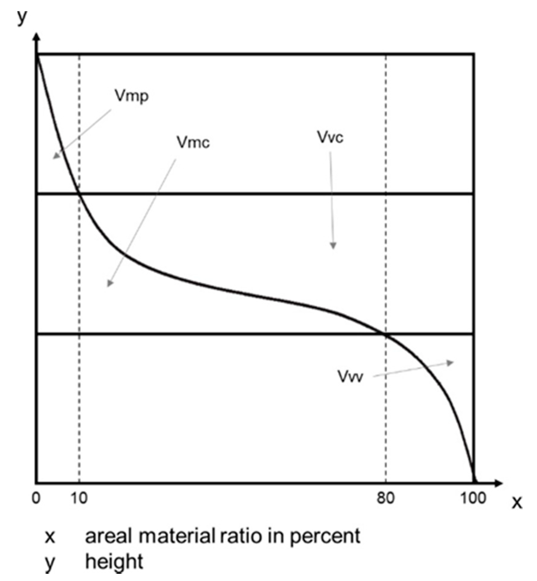
  • Pmp (Vmp) is the peak material volume;
  • Pmc (Vmc) is the difference in material volume between p and q material ratios (by default p = 10% and q = 80% [33]);
  • Pvc (Vvc) is the difference in void volume between p and q material ratios (p = 10%, q = 80%);
  • Pvv (Vvv) is the void volume.
The fractal dimension of profiles
Fractal dimensions can describe the complexity of natural phenomena where similar structures that are repeating at different scales are called self-affine structures [34]. Highly self-affine structures can be considered complex or “rough”. The basic concept of fractal dimensions is that the more self-affine or self-similar a profile is, the higher its fractal dimension becomes, and this has led to the idea that it could be used as a measure for the roughness of a profile or area [35]. This measure is inherently different from classic profile parameters and was therefore included in the current work as an alternative parameter for characterizing surface texture. One of the most used methods for evaluating the fractal dimension of a profile for roughness considerations is the “roughness-length” method, first proposed by Malinverno [36].
The calculation of the fractal dimension of a profile is based on dividing the profile into “windows” of different length and calculating the root mean square (RMS) value for the window length:
R M S ( w ) = 1 n w i = 1 n w 1 m i 2 j     w i ( z j z ¯ ) 2
where w is the window length in points, n w is the number of windows at that window length, m i is the number of points within the current window, z j is the profile heights within a window, and z ¯ is the mean profile height within a window. The window lengths used were w = 1 n d , where n d represents the length divider and were 2, 4, 8, 16, and 32 in this work. With an overlap of 50% between windows, the number of windows for each n d became n w = 3, 7, 15, 31, and 61, respectively. An RMS-value was calculated for each of the n w window sets. The resulting RMS-values were then plotted against the window lengths on a log-log plot as shown in Figure 5 for the channel with Dnom = 3 mm. H is the slope of a linear trend line on the Log(w) vs. Log (RMS) plot.
Finally, the fractal dimension FracDim of the investigated profile can be calculated as:
F r a c D i m = 2 H

2.3.1. Qualitative Comparison of Dross Formation and Profile Parameters

The main characterization performed in this work was focused on the investigation of the possible correlation of the selected surface profile parameters with the dross formation. For this purpose, polar plots were used to show an intuitive representation of the local estimations of each computed parameter for each of the investigated channels. Figure 6a shows an example of a polar plot of the parameter Pa as a function of the internal local orientation β (or Pa(β)) for Dnom = 3 mm. Note that the scale is radial and that the unit is in µm. Figure 6b shows a sketch of the definition of the local orientation β where β = 180° towards the build direction. Each of the generated polar plots for each of the 12 parameters will be compared to the representative surface deviation map of the investigated channel. An example of such a surface deviation map for Dnom = 3 mm can be seen in Figure 7a.

2.3.2. Roughness Prediction Model and Geometry Estimation

The calculated Pa-values for each of the investigated channel sizes were used to generate a simple roughness prediction model as a function of the local orientation (β) and the channel diameter (D), namely Pa (β, D). The model was created by collecting all Pa-values in the same data plot and using channel 6 mm A as the representative for the 6 mm channels. While the resolution of the estimated Pa-values was well over 1 per degree along β, the Pa-values were only calculated directly for the corresponding channel sizes. Therefore, linear interpolation was used to fill the gaps between the analyzed channel diameters leading to the generation of a simple Pa (β, D) prediction model, which is shown in Section 3.3.1.
As an application relevant validation of the used surface texture characterization methodology, the model was used to modify an ideal (cylindrical) CAD geometry of a channel with Dnom = 6 mm following a point cloud manipulation approach first presented by [26]. The approach is aimed at utilizing roughness prediction models to modify the geometry of nominal channel designs based on their expected outcome when manufactured using LPBF.

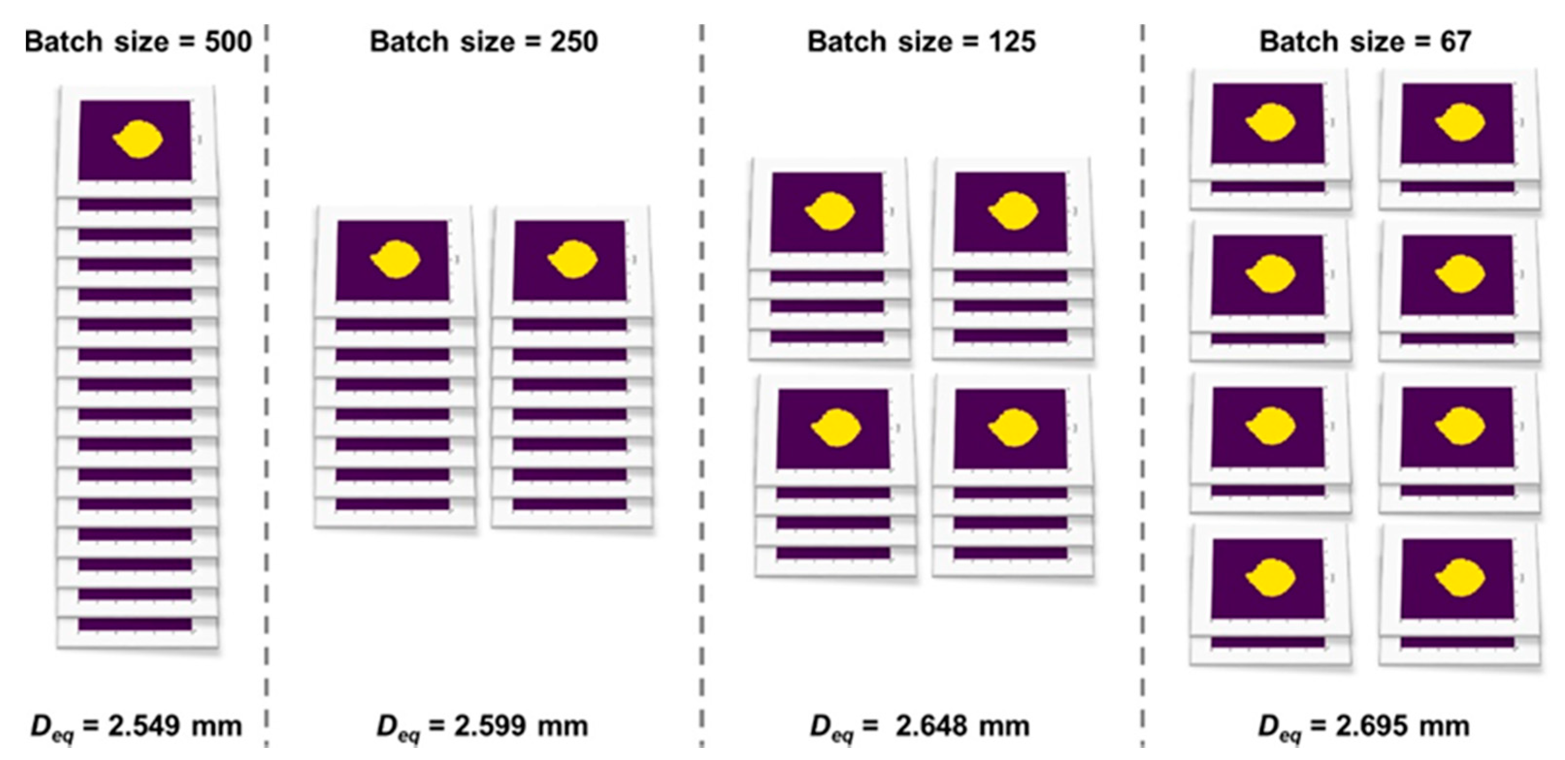
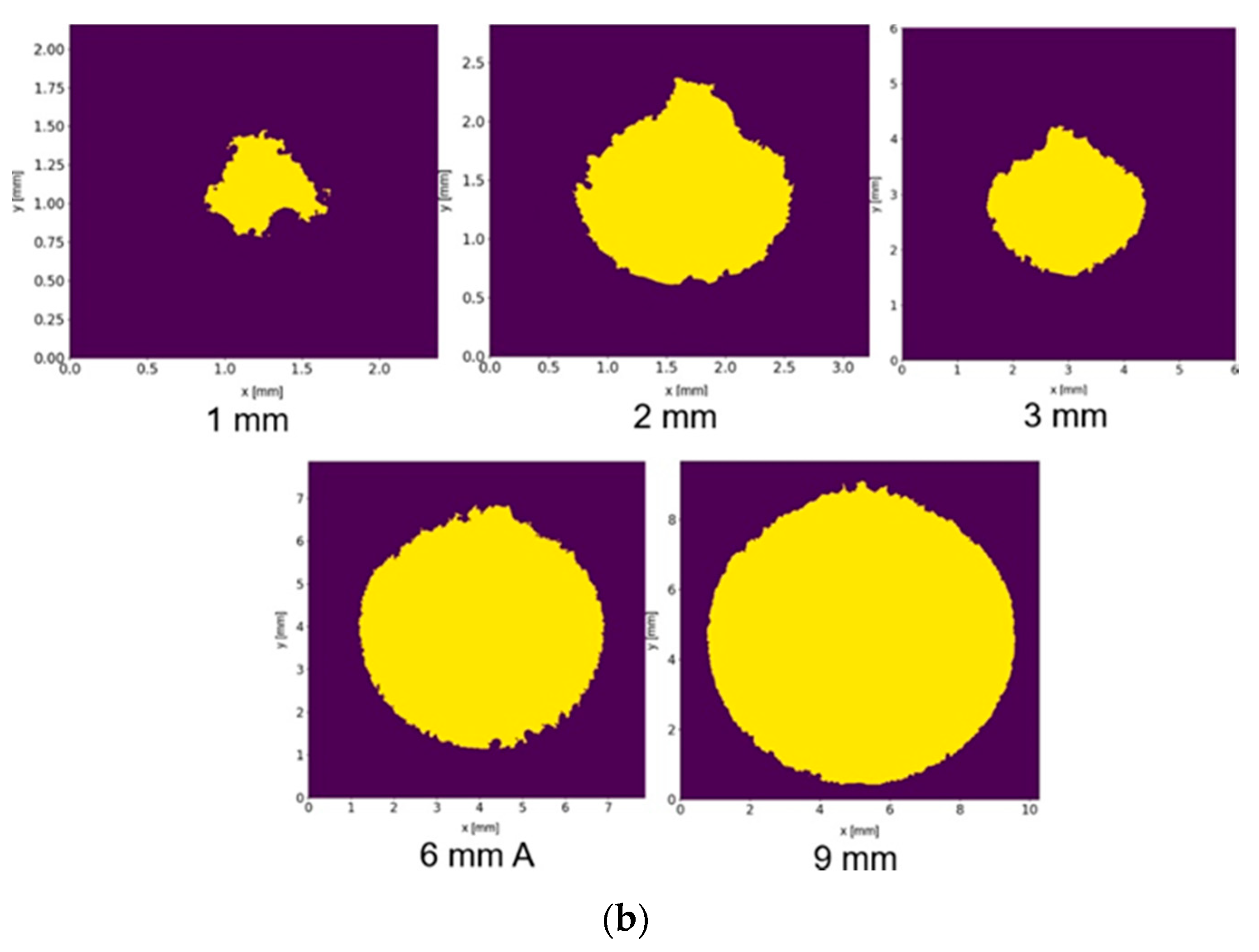
2.4. Equivalent Diameter of the Unobstructed Cross-Sectional Area

When designing cooling channel systems, the channel diameter is selected based on the expectation of a given flow through-put, but when considering LPBF channels, the unobstructed cross-sectional area (or equivalent diameter) may be far from the nominal design. Figure 7a shows a 3D visualization of the Dnom = 3 mm channel investigated using the default image stack size of 500 images, as discussed in Section 2.2. Figure 7b shows a view of the cross-sectional area obtained by stacking all 500 images on top of each other and projecting a “light” through, corresponding to the yellow area. Both figures have been oriented to correspond to the defined orientation, shown in Figure 6b, with the build direction being towards β = 180°. By comparing Figure 7a,b it can be seen how the contour of the white center in Figure 7a is closely represented by the contour of the yellow area in Figure 7b, except for the perspective view in Figure 7a.
The current work suggests a methodology for estimating the equivalent diameter (Deq) of the unobstructed cross-sectional area as a function of the channel length. The approach was similar to that of fractal dimensions but instead of considering window lengths, in this proposed methodology, batch sizes containing a set number of images were considered. Figure 8 shows an example of one stack of images that was divided into smaller batches. For each batch size, an average value for Deq could be calculated, giving an estimate of Deq at the corresponding length. For a batch size of 125 images, representing a length of 125 images × 9 µm/image = 1.13 mm, the estimated equivalent diameter was Deq = 2.648 mm, using the following equation:
D e q = i = 1 N 4 A i π N
where Ai is the area calculated from the pixels corresponding to the unobstructed cross-sectional area (the yellow area in Figure 7b) from batch i, and N is the stack divider. The initial image stack with a batch size equal to 500 was divided into smaller batches using the following eight stack dividers: 1, 2, 4, 8, 16, 32, 64, 128, and 256.
Figure 9a shows the nine points plotted with a linear fit, a second-order polynomial fit, a third-order polynomial fit, and a natural logarithmic fit, using increasing weights of [1, 10, 100, 103, 104, 105, 106, 107, 108] with length, for the Dnom = 3 mm channel. The logarithmic fit is shown to be highly representative of the calculated Deq-values. The shown estimation was based on the default maximum batch size of 500. Moreover, it was investigated if this batch size was adequate in predicting Deq for longer channel lengths. The investigation was conducted by considering the 500 images as a “normal” stack size and comparing it to a larger stack size. The larger stack size consisted of all the good quality images available for the channel. For Dnom = 3 mm a total of 1890 cross-sectional images were used (the remaining 110 images available did not have a high enough quality). The data of the two stacks can be seen in Figure 9b, together with the logarithmic fits. For the fit of the large data set, no weighing was used. A simple quantitative comparison between the two stack sizes was performed by calculating the average difference in the estimated Deq-value for the two stacks sizes over a length of 50 mm. The resulting deviation was 1.4%, proving a good agreement between the two calculations. Using the default stack size of 500 images can then be considered enough to give a good approximation of the actual Deq. The points representing the longest lengths in Figure 9 were calculated using stack dividers of 1 and therefore have no standard deviations.

3. Results and Discussion

The results of the characterization are presented and discussed in the following. In Section 3.1, a qualitative comparison of the investigated channels is shown. Section 3.2 includes a presentation of the general geometric and surface texture characterization of the investigated channels together with the generated estimations for Deq. Section 3.3 is focused on the investigation of the possible correlations between the computed surface profile parameters and the dross formation. In addition, it also includes a description of the simplified roughness model Pa (β, D), enabling prediction of the expected internal roughness for aluminum LPBF channels in a size range similar to the channels of this work and produced under similar process conditions. Finally, the roughness model is used to predict the geometry of a CAD design. The predicted geometry is then compared to the surface deviation map of an analyzed channel of the corresponding geometry.

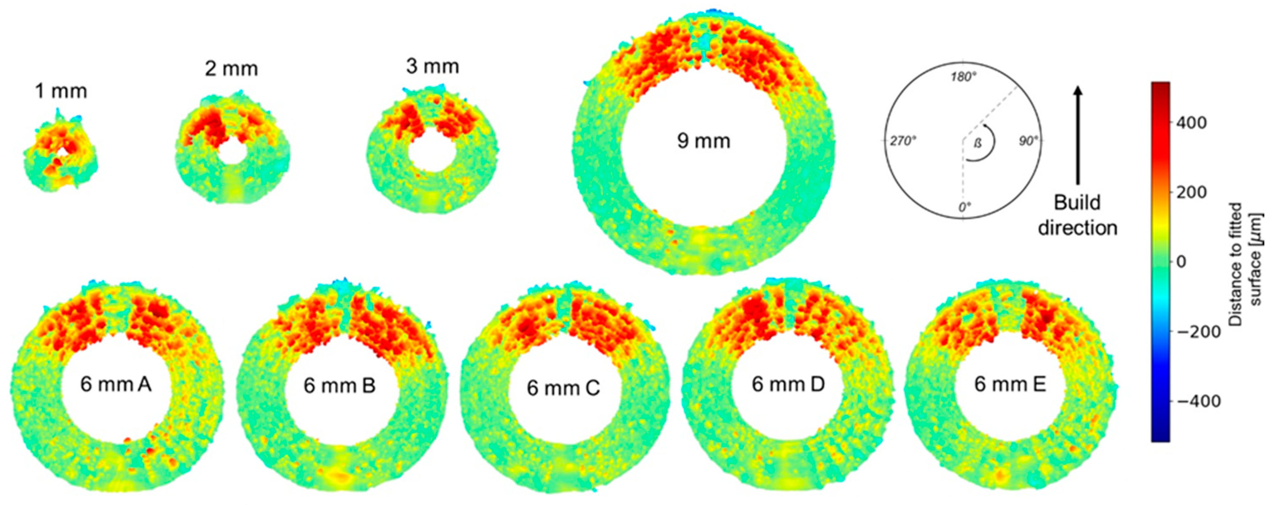
3.1. Qualitative Overview

Figure 10 shows a surface deviation map overview of all the investigated channels. The sizes of the channels are scaled to the approximate relative sizes, enabling a qualitative comparison.
At around β = 180°, it can be seen how dross formation is significantly reduced for all investigated channels except Dnom = 1 mm. This is likely due to the surface being identified as a down skin surface. A down skin surface is typically made with reduced power and scan speed to reduce the locally accumulated heat. A reduction in the locally accumulated heat could result in the observed reduction in sintered particles. The experimental and numerical work conducted by Khan et al. on small circular LPBF geometries, made in AlSi10Mg, supports this observation [37]. Their work showed a significant influence from changing down skin parameter settings such as laser power, scan rate, and hatch spacing on the dross formation in LBPF manufactured channels with a diameter of 0.5 mm and a build orientation perpendicular to the build direction.
From the view through the channels, some qualitative deductions can be made. First, it can be seen how all channels, except the Dnom = 1 mm channel, follow a general dross formation pattern with regions of high dross formation on both sides of β = 180°. This is in contrast to the dross formation pattern observed in steel LPBF channels [29,38] where the dross formation was continuous from β = 90° to β = 270° and with maximum dross at β = 180°. This discrepancy could be caused by the use of different process parameters at the down skin surfaces. The method of locally optimized process parameters might also be affecting steel and aluminum powder differently. The difference observed in the dross formation pattern could be due to the difference in thermal conductivity between aluminum and steel. The higher conductivity of aluminum allows for a larger degree of thermal diffusivity and could result in less heat accumulation at the top of the overhanging section, and thus less dross formation. The observed trend shows that in the range of β ˂ 90° or β ˃ 270°, dross formation is generally minimal. A few scattered sintered particles and particle agglomerations are found on the upward facing surface. The sintered particles are mostly seen around β = 45°, which could be due to the influence of the stair-casing effect, leading to further retainment of sintered particles [38]. The dross formation is seemingly increasing from β = 90° towards β = 180° until it abruptly reaches the onset of a low-dross area forming an upside-down “valley” between two “hills”. While all investigated channels with Dnom ≥ 2 mm follow the same dross formation pattern, the Dnom = 1 mm channel is experiencing close to randomly distributed dross formation. This could be due to the small size of the channel and the possibility of increased local heat accumulation in the adjacent powder. Due to the size of the channel, this accumulated heat could be affecting every part of the channel contour leading to increased particle sintering. Finally, it can be seen how the angular widths (β) of the two dross formation “hills” are increasing with decreasing channel diameter.

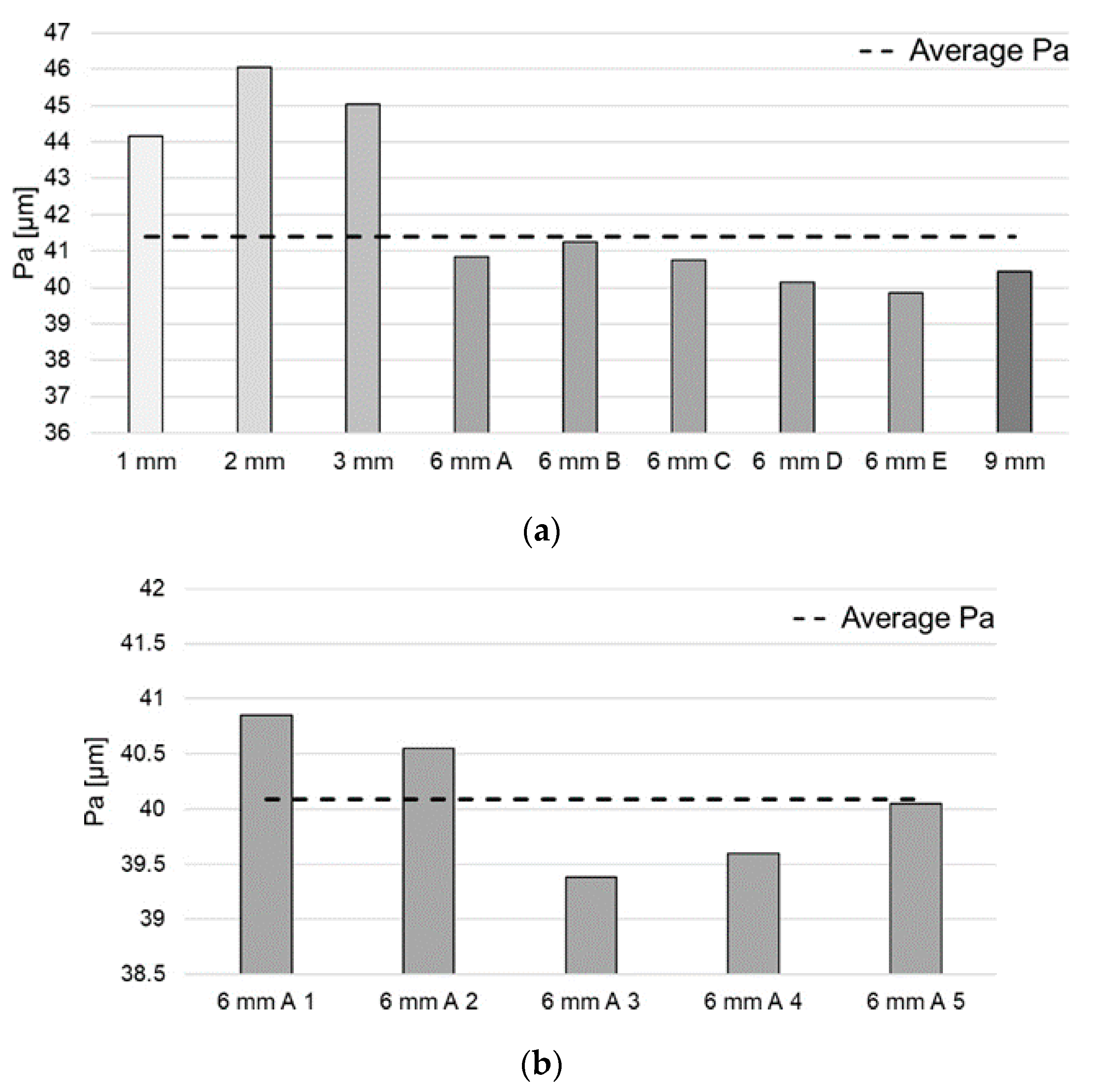
3.2. Geometric and Surface Texture Characterization

Figure 11 shows the difference in equivalent and nominal diameters for the nine investigated channels, together with unobstructed views of the five investigated channels with different diameters.
Figure 11a shows how the difference (DeqDnom) is close to being constant for channel diameters of Dnom ≥ 3 mm. The reduction in the unobstructed cross-sectional area follows a power law with increasing channel diameter, which is also to be expected since A = ( D 2 ) 2 × π   . Figure 11b shows the unobstructed cross-sectional area of the investigated channel sizes. The cross-sectional views show a similar dross formation trend, how it is different for Dnom = 1 mm, and how the peak-valley-peak signature of dross formation is becoming decreasingly apparent from Dnom = 2 mm to Dnom = 9 mm.
Figure 12a shows the overall channel average Pa-values calculated for all investigated channels. The average Pa-values divided the channels into two distinctive groups: 1 mm ≤ Dnom ≤ 3 mm and 6 mm ≤ Dnom ≤ 9 mm. The calculated channel averages are similar within the two groups indicating a shift in the magnitude of average roughness between Dnom = 3 mm and Dnom = 6 mm. Apart from this size effect, it was found that within the group separated into “small” and “large” channels, a similar average roughness can be expected, irrespective of the nominal channel diameter. Figure 12b shows the results obtained from the five repeated X-ray CT scans of the 6 mm A channel. The results can then be compared to the other five 6 mm channels (Figure 12a), to investigate the repeatability of the production process.
The overall average Pa-value together with the associated standard deviation, together with the corresponding values of the repeatability investigations, can be seen in Table 2. By comparing the standard deviations of the Pa-values, it can be seen how the process and analysis repeatability are not significantly different, although when comparing the standard deviation of the obtained Deq-values, the standard deviation of the repeated CT scans is half that of the process-induced standard deviation. Part of the process repeatability discrepancy may be attributed to build platform positioning effects, which have been found in other works to affect the roughness of produced parts and may therefore also affect the diameter [39].

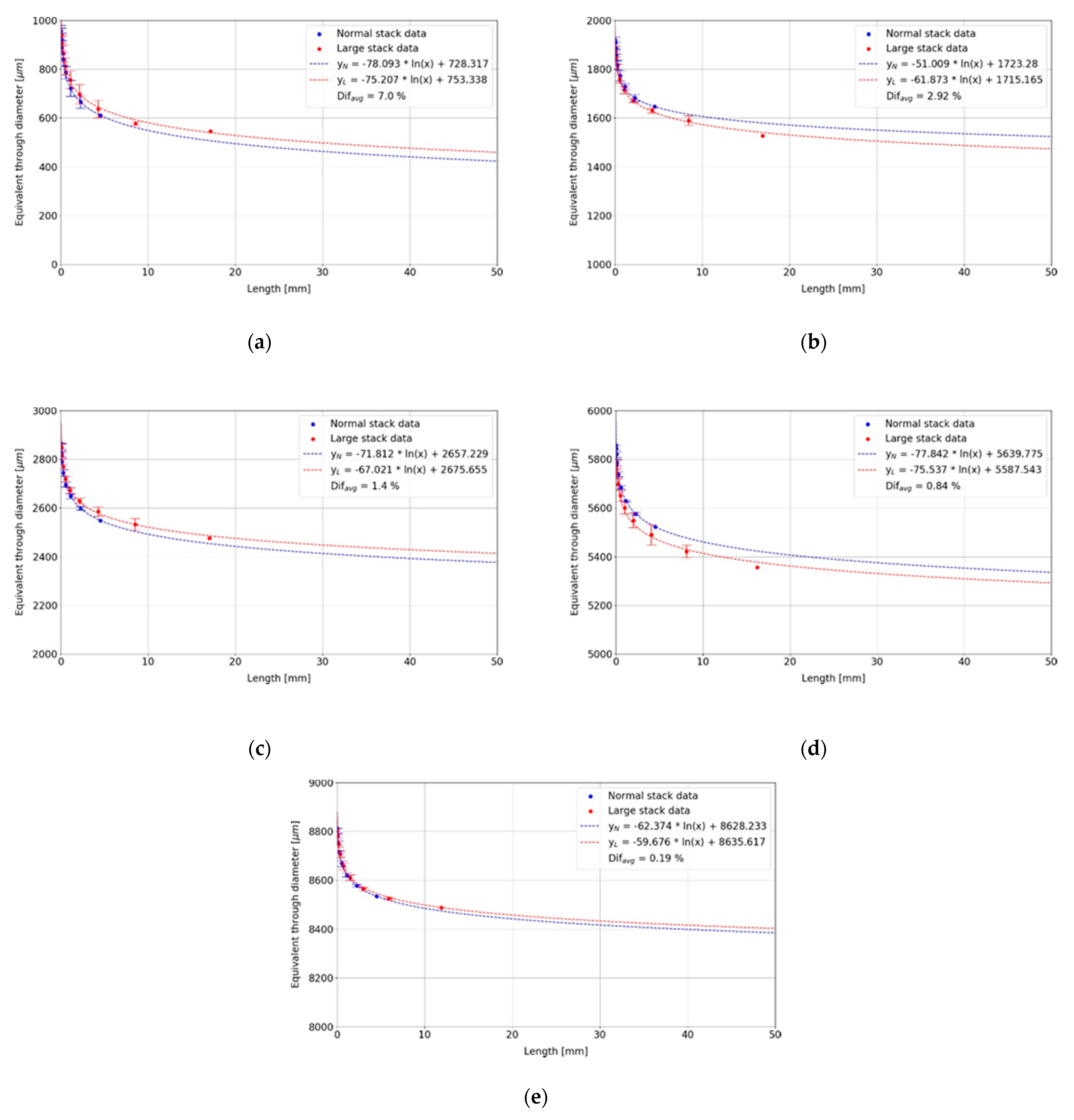
Estimation of the Equivalent Diameter Deq

The estimation of the equivalent diameter for the investigated channels as a function of channel length can be seen in Figure 13. As discussed in Section 2.4, the reduction in Deq closely follows a logarithmic trend for all the investigated channel sizes.
The influence of stack size was investigated for all channel sizes to test the estimation methodology. The estimated Deq-values, at a length of 1000 mm, are shown in Table 3, together with the mean difference in percent over the visualized estimation length of 50 mm (Figure 13). The absolute differences in predicted Deq at 1000 mm length for the two stack sizes are between 0.026 and 0.083 mm across the investigated channel sizes with the largest relative differences found for the smallest diameters. This was also the case for the mean differences (in percent) over a length of 50 mm.
The predicted reduction over a length of 50 mm is between 500 and 700 µm for both stack sizes with no clear relation to channel size, indicating that the reduction in Deq could be similar at all diameters and is not dependent on the selected channel size, but rather on the chosen process parameters and material.

3.3. Correlation of Surface Profile Parameters and Dross Formation

This subsection is dedicated to the investigation of the possible correlations between the selected surface profile parameters (see Section 2.3) and the dross formation. Figure 14 shows an overview of polar plots visualizing the computed profile parameters at every local orientation (β) for the investigated channel, 6 mm A. For each of the other investigated channel sizes, the polar plots together with the corresponding generated surface deviation map may be found in Figure A1 in the Appendix A. The average value of the profile parameter shown in each polar plot is given at the top right corner of the plots. The channels 6 mm B, 6 mm C, 6 mm D, and 6 mm E are not reported as their results are very similar to those obtained for channel 6 mm A.
Figure 14 shows a profile parameter comparison for the Dnom = 6 mm channel. Polar plots for Pa, P10z, Pq, Pz, Pp, Pmc, and Pvc show similar trends. This observation was found to be true for all investigated channels but is more evident in the larger channels with Dnom ≥ 3 mm. By comparing the abovementioned parameters with the surface deviation map shown in Figure 14, it becomes apparent that the magnitude of the calculated parameters can be considered connected to the magnitude of the surface deviation maps, which in essence shows the level of dross formation in the channels. This observation indicates that it can be expected that areas with higher dross formation will also have higher surface roughness. The seven parameters mentioned above can all be considered as suited to characterize the variation of the magnitude of surface texture in different axial profiles of internal channels, especially Pa, P10z, and Pq are practically interchangeable for this purpose. For convenience, it was decided to use Pa as the main parameter for characterizing the variation of surface texture magnitude as a function of the local orientation β.
Pmp and Pvv were found to be close to inversely related as would be expected from the definitions. Pvv even showed resemblance to the seven parameters mentioned earlier that were found usable in the characterization of the roughness magnitude. Pmp allows determining if a profile had maxima relative to the general roughness of the surface. Two examples of this can be found in Figure 14 around β = 5°, β = 185°, and β = 270° where Pmp spikes and indicates that the extracted profile at that local orientation has large peaks relative to the profile heights. This inference can be confirmed by inspection of the surface deviation map at the same β-orientations, where generally “flat” sections are found with a few agglomerations acting as local maxima on an extracted profile.
Psk, or the “skewness” of the profile, is used to characterize the bias of the profile around the mean line. For channels with Dnom ≥ 6 mm, Psk is negative when the roughness is high and positive when the roughness is low. This indicates that in areas with high roughness the profile is skewed above the mean plane. For the smaller channel sizes, this trend is not as clear. The practical use of Psk is not straightforward, whereas Pku, which reacts much stronger to extremes, can be used very similar to Pmp to identify the spikiness of a profile, i.e., to what degree the profile consists of deep valleys and high peaks (Pku > 3) or shallow valleys and soft hills (Pku < 3). Flat sections (as found at β = 0°) tend to yield unreliable results for Pku as can be seen in Figure 14. While Pku is similar to Pmp, extremes are affecting Pmp more strongly. This means that Pku is better for general spikiness of a profile and Pmp is good for evaluating irregular height distributions such as flat surfaces suddenly having an agglomeration resulting in a high profile peak.
The final profile parameter investigated in this work was the fractal dimension (FracDim). It was found that the roughness trend yielded by the fractal dimension, calculated using the RMS method, was opposite to that of the parameters found to adequately characterize the roughness magnitude. In other words, a high fractal dimension was typically calculated for a profile with low Pa-values. The heights of a typical profile extracted through a section with dross formation will not be self-similar at different scales, which will not translate into a “complex” profile according to the self-affinity principle of fractal dimensions. On the other hand, when a section is free of random particles and agglomerations, the extracted profile will be highly self-similar resulting in a high fractal dimension. This can be confirmed by for example inspecting Figure 14 where a large β-range is almost free of sintered particles (280° < β ˂ 330°), which results in calculated fractal dimensions of around 1.7. Similarly, a small section at around β = 170° is almost free of random extremes, resulting in a fractal dimension of up to 1.7. This trend could mean that the fractal dimension can be used to characterize the degree of random particle sintering at a given β for LPBF channels and, therefore, identify key orientations with the tendency to have large and randomly distributed sintered particle agglomerations.
Table 4 shows the calculated average profile parameter values for each of the investigated channels. The investigated channels can generally be divided into two groups: group 1 consists of smaller channels with Dnom ≤ 3 mm and group 2 consists of larger channels with Dnom ≥ 6 mm. Within the two groups, each group has approximately the same quantitative average profile parameter values calculated for Pa, P10z, Pz, Pq, and Pp.
Psk is positive for Dnom ≤ 3 mm and close to zero for Dnom ≥ 6 mm, indicating a generally more even distribution of peaks and valleys in larger channels. Pku is generally above 3 for all channels, except for Dnom = 2 mm, indicating a general spikiness of the surface roughness in aluminum LPBF channels.
The average fractal dimension is increasing with decreasing channel diameter. This is likely related to dross formations and particle agglomerations taking up more of the overall space in the channel.
The profile versions of the material volume parameters, Pmc, Pvc, Pmp, and Pvv are “area” dependent and, therefore, the parameters can only be used to compare values within the same channel size. For Dnom = 6 mm, it can be seen how the parameters are varying slightly between the five investigated channels (A, B, C, D and E) with the most variation being observed in Pmp, indicating that the extremes of the height distributions are mostly affected by variation in the manufacturing process, which is also to be expected.

3.3.1. Obtained Roughness Model and Resulting Geometry Predictions

The surface topography characterization, performed using 12 different surface profile parameters (see Section 3.3), showed that Pa can be considered as an appropriate parameter for describing the dross formation and magnitude of the associated roughness. The simple roughness prediction models obtained and the corresponding results, from following the approach described in Section 2.3.2, can be viewed in Figure 15.
Figure 15a shows the roughness prediction model. The predicted roughness and geometry of a perfect CAD channel geometry with Dnom = 6 mm, together with the surface deviation map of the 6 mm A channel, can be seen in Figure 15b,c. Figure 15b shows that the roughness and shape are well predicted. The contour of the white area within the modeled channel (Figure 15b) is closely representing the contour of the white area within the X-ray CT characterized channel (Figure 15c), indicating a good geometric reproduction by the prediction methodology. The overall width of the dross formation area is slightly overestimated just as the local heights of the peaks are underestimated. This is likely due to the model being based on average Pa-values, which will smoothen out the predictions. The shown comparisons confirm the applicability of the parameter Pa for providing an appropriate description of the roughness and dross formation trends observed in the investigated aluminum LPBF channels.

4. Conclusions

In this work, nine LPBF aluminum channels were characterized in terms of equivalent channel diameters and surface topography, using X-ray CT and image analysis. The work presents a simple methodology for estimating the equivalent diameter (Deq) of the unobstructed cross-sectional area as a function of channel length, enabling the optimization of channel designs.
An overview of surface deviation maps allowed for the description of a distinct roughness and dross formation trend in the observed channels. The trend might have been formed due to the use of different process parameters at surfaces identified as down skin/overhanging surfaces. The dross formation at overhanging areas was found to follow a reverse “camelback” trend with low to no dross formation around β = 180° within an angular width of approximately 10° and high dross formation on both sides of the low dross area. The total reduction in Deq at the investigated length was found to be close to constant for the channel sizes Dnom ≥ 3 mm. Furthermore, it was found that Deq could be estimated as a function of the channel length and that the reduction followed a logarithmic trend for all investigated channel sizes.
The analysis of surface texture using different surface profile parameters resulted in the following key findings:
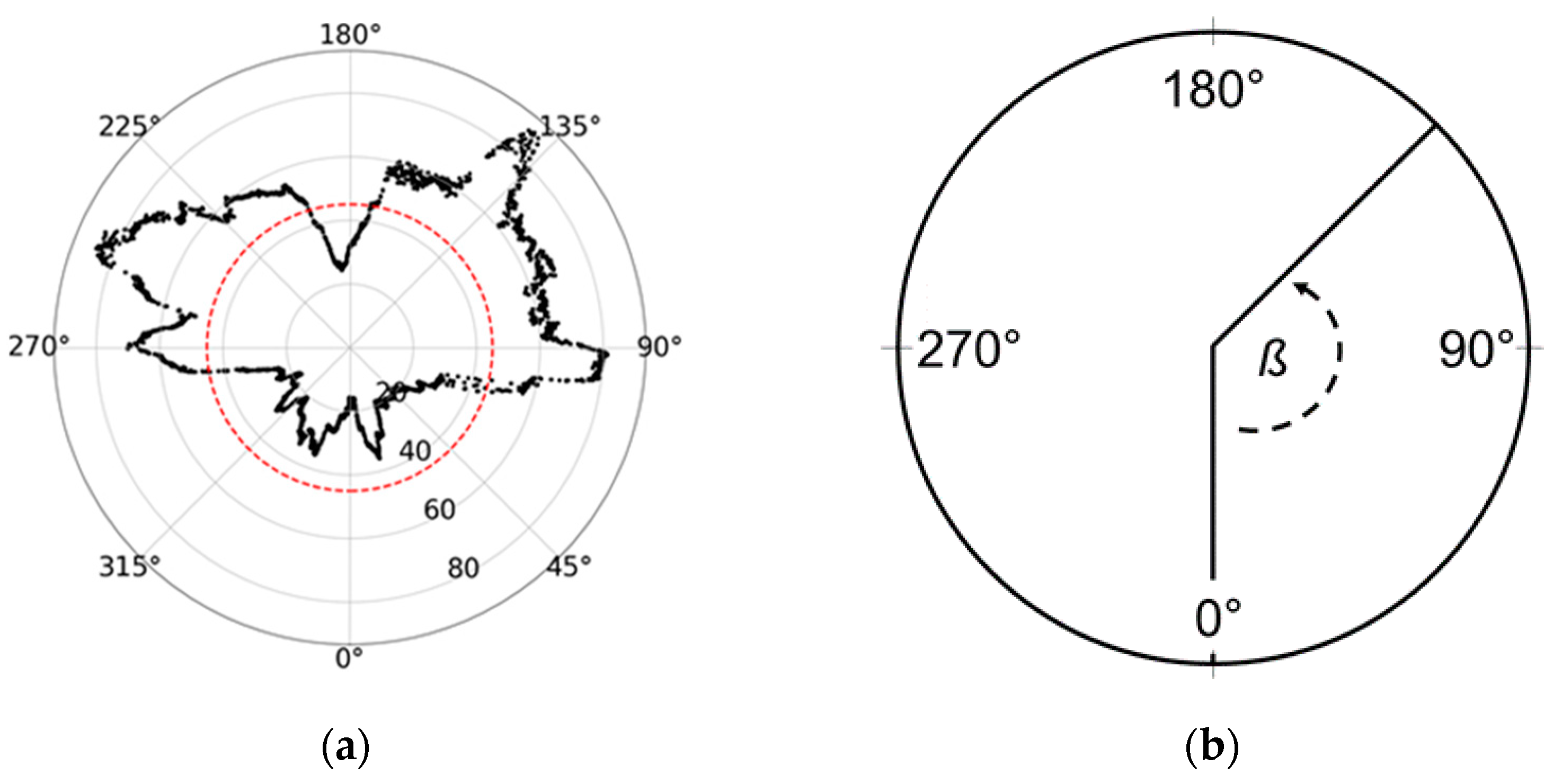
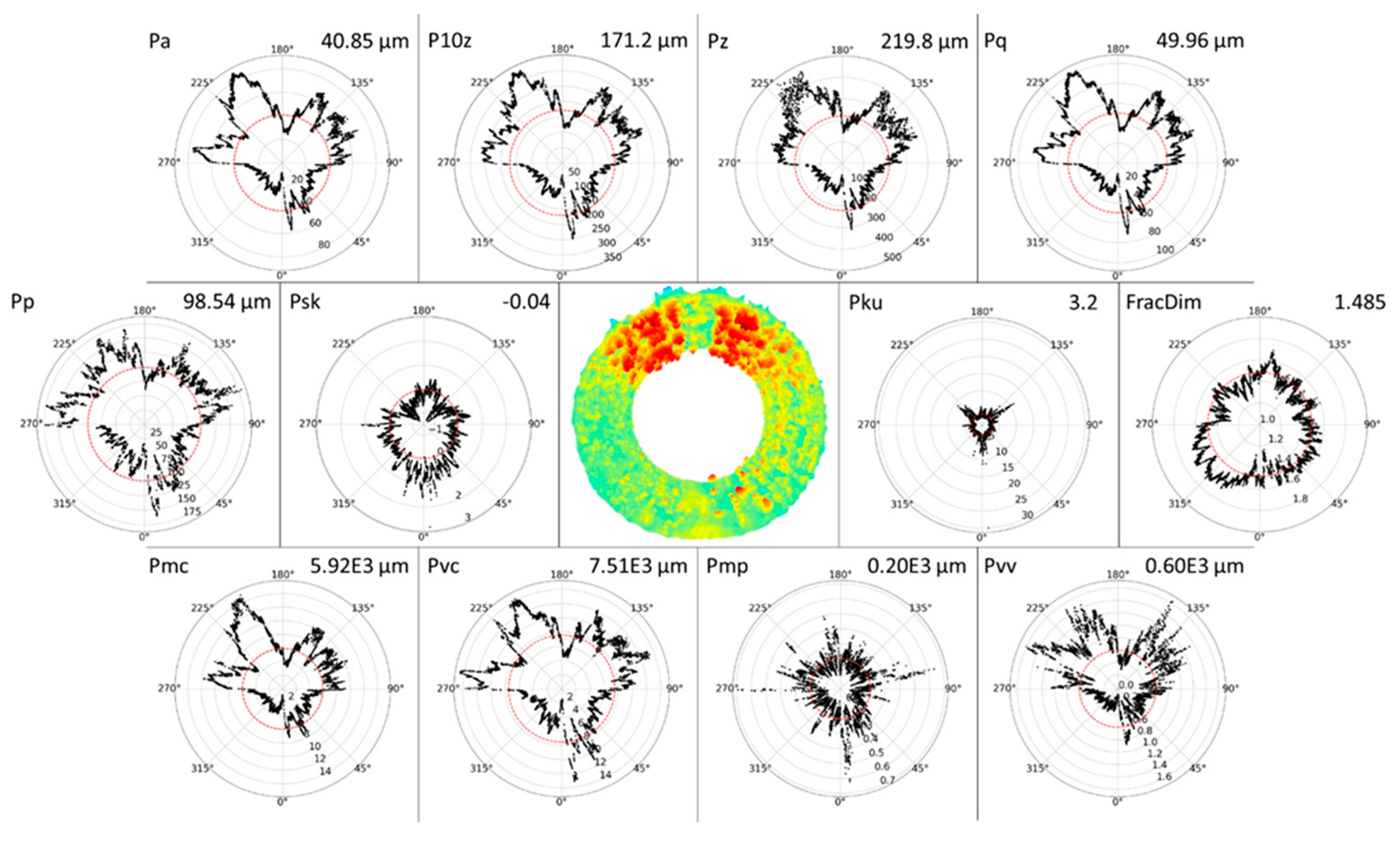
  • Pa, P10z, and Pq are interchangeable for the specific purpose of quantifying the variations in the surface texture level depending on the angular local orientation β, hence describing the dross variation around the channel periphery, with only a scaling factor separating the parameters quantitatively;
  • Pz, Pp, Pmc, and Pvc are closely related to the above;
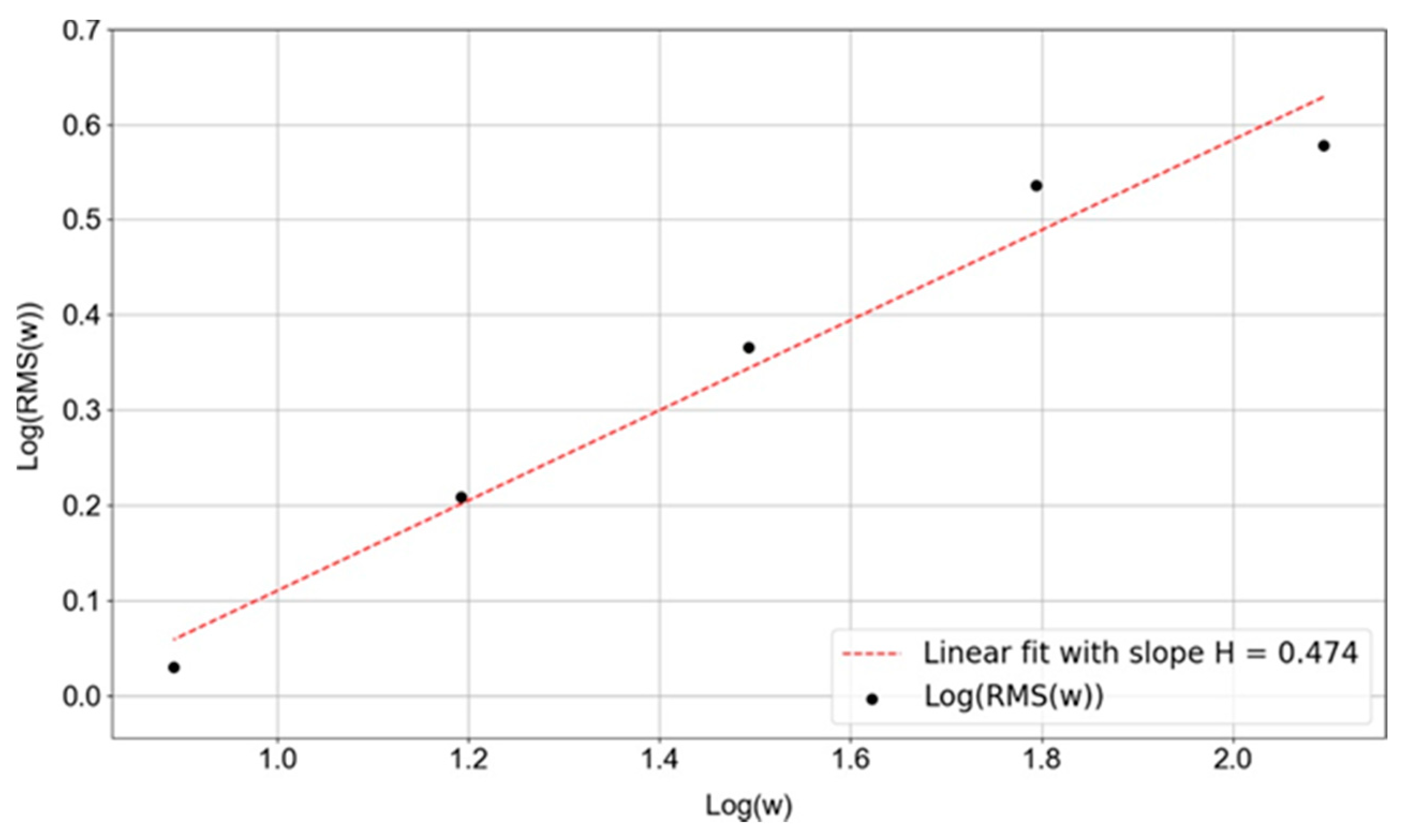
  • Pku and Pmp are useful parameters for the characterization of the peak-valley nature of the profiles. Pmp and the fractal dimension of a profile may be used to characterize the degree to which a surface is affected by local distributions of sintered particles and agglomerations;
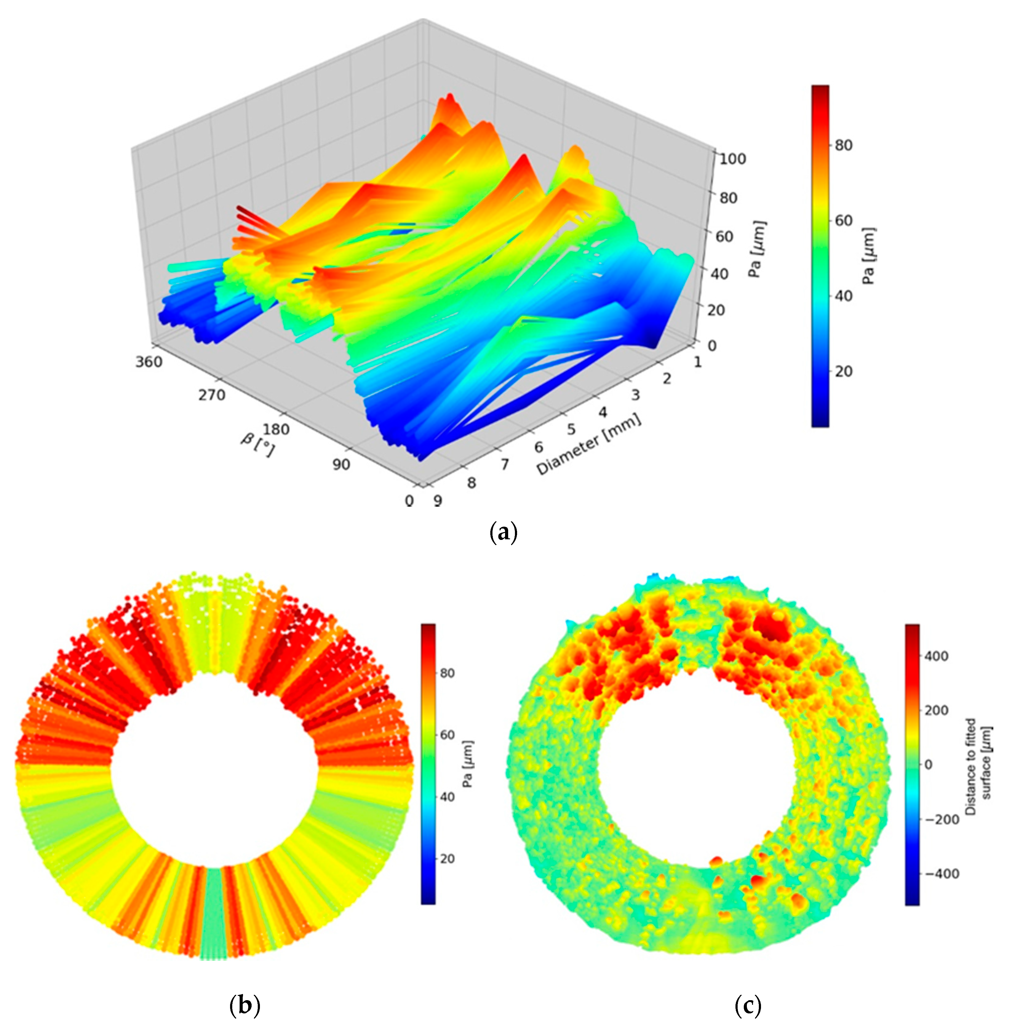
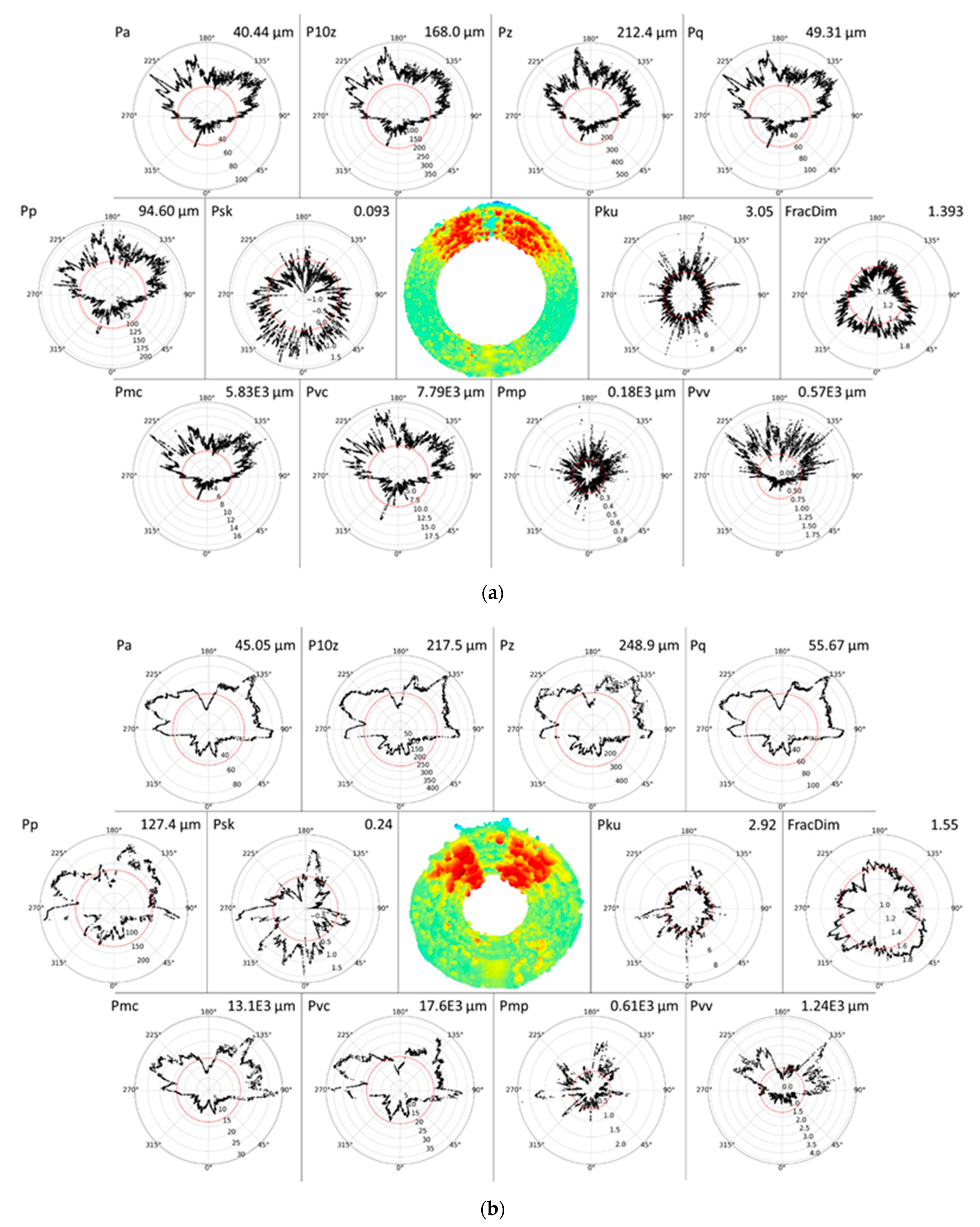
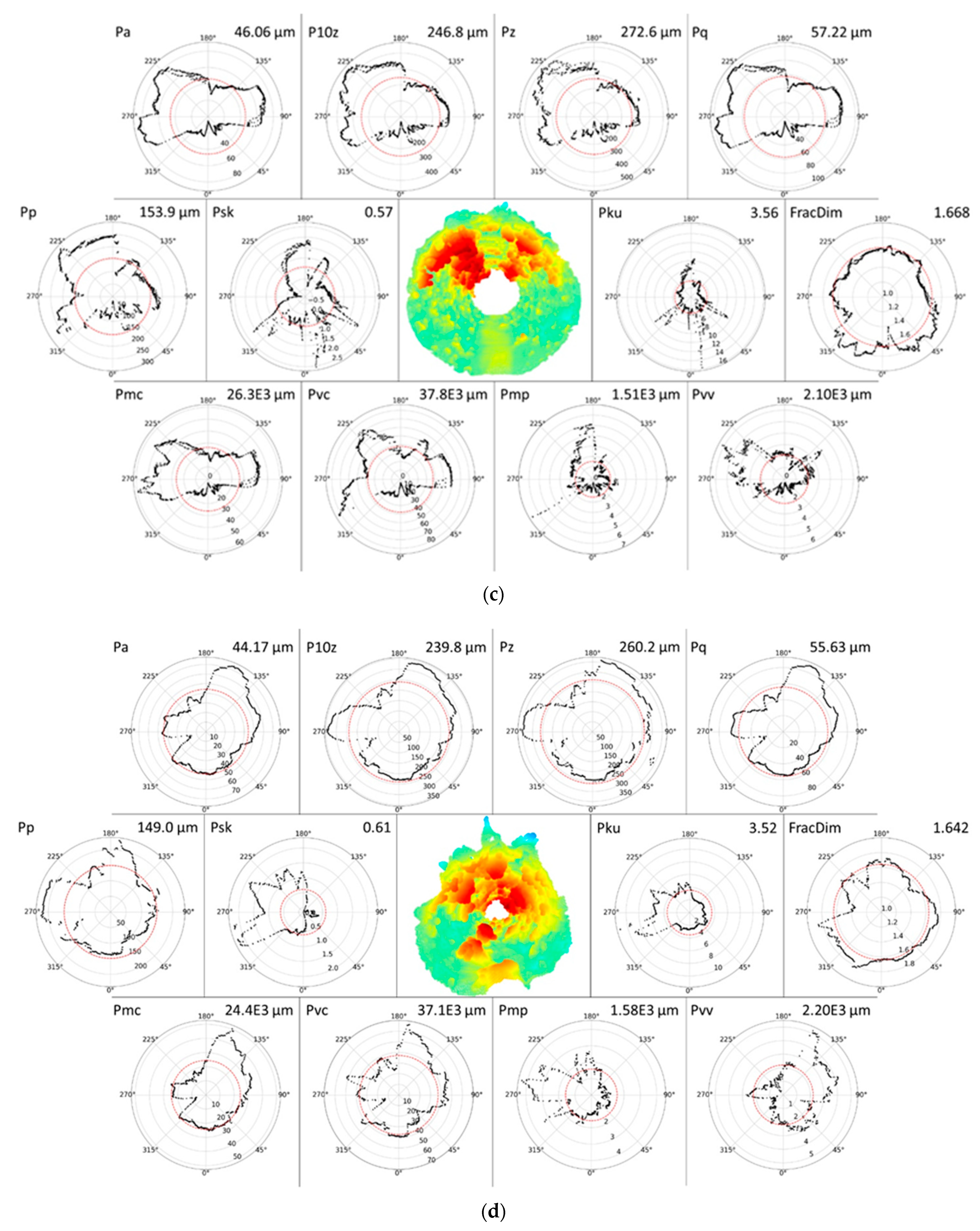
  • The channels could be divided into a group for smaller channels Dnom ≤ 3 mm and a group for larger channels Dnom ≥ 6 mm in terms of quantitative characterization of the observed roughness. The group with smaller channels had an average Pa of around 10% higher than that of the larger channels.
While the current work did not intend to develop new parameters, the use of existing parameters and their appropriateness was sought to be investigated. The possible connections observed in this work between the selected surface profile parameters and dross formations and the presence of particles and agglomerations on the internal channel surface could help move towards a better understanding of the appropriate parameters for characterizing dross formation and surface texture in all AM channels.
The appropriateness of using Pa as the measure for variations in the surface texture level depending on the angular local orientation, while being correlated with dross formation, was validated by the generation of a simple roughness prediction model Pa (β, D). The roughness model was successfully used to generate a modified CAD design of a Dnom = 6 mm with information on the predicted roughness and dross formation.
Future work is planned to (i) investigate the applicability of the proposed methods on channels with different geometries and made under different processing conditions and (ii) determine the uncertainty of CT surface texture measurements.

Author Contributions

Conceptualization, C.G.K., F.Z. and S.M.; methodology, C.G.K.; software, C.G.K.; validation, C.G.K.; formal analysis, C.G.K.; investigation, C.G.K. and F.Z.; resources, F.Z. and S.C.; data curation, C.G.K.; writing—original draft preparation, C.G.K.; writing—review and editing, F.Z., S.M., S.C. and J.H.H.; visualization, C.G.K.; supervision, S.M. and J.H.H.; project administration, S.M.; funding acquisition, S.M. and J.H.H. All authors have read and agreed to the published version of the manuscript.

Funding

This research was funded by the Innovation Fund Denmark Grand Solutions project “MADE Digital”, grant number 6151-000068.

Institutional Review Board Statement

Not applicable.

Informed Consent Statement

Not applicable.

Data Availability Statement

The analyzed datasets used during the current study are available from the corresponding author on reasonable request.

Acknowledgments

The Danish Technological Institute is thankfully acknowledged for manufacturing the LPBF aluminum channels investigated in this work.

Conflicts of Interest

The authors declare no conflict of interest.

Appendix A

Figure A1. (a) 9 mm. (b) 3 mm. (c) 2 mm. (d) 1 mm.
Applsci 11 04304 g0a1aApplsci 11 04304 g0a1b

References

  1. Armillotta, A.; Baraggi, R.; Fasoli, S. SLM tooling for die casting with conformal cooling channels. Int. J. Adv. Manuf. Technol. 2014, 71, 573–583. [Google Scholar] [CrossRef] [Green Version]
  2. Han, Q.; Gu, H.; Soe, S.; Setchi, R.; Lacan, F.; Hill, J. Manufacturability of AlSi10Mg overhang structures fabricated by laser powder bed fusion. Mater. Des. 2018, 160, 1080–1095. [Google Scholar] [CrossRef]
  3. Wang, D.; Yang, Y.; Yi, Z.; Su, X. Research on the fabricating quality optimization of the overhanging surface in SLM process. Int. J. Adv. Manuf. Technol. 2013, 65, 1471–1484. [Google Scholar] [CrossRef]
  4. Snyder, J.C.; Stimpson, C.K.; Thole, K.A.; Mongillo, D. Build Direction Effects on Additively Manufactured Channels. Vol. 7B Struct. Dyn. 2015, 138, 1–8. [Google Scholar] [CrossRef]
  5. Chen, H.; Gu, D.; Xiong, J.; Xia, M. Improving additive manufacturing processability of hard-to-process overhanging structure by selective laser melting. J. Mater. Process. Technol. 2017, 250, 99–108. [Google Scholar] [CrossRef]
  6. Moody, L.F. Friction Factors for Pipe Flow. Trans. Am. Soc. Mech. Eng. 1944, 66, 671–681. [Google Scholar]
  7. Stewart, M. Fluid flow and pressure drop. In Surface Production Operations; Elsevier BV: Amsterdam, The Netherlands, 2016; pp. 343–470. [Google Scholar]
  8. Chhabra, R.; Richardson, J. Flow in Pipes and in Conduits of Non-circular Cross-sections. In Non-Newtonian Flow and Applied Rheology; Elsevier BV: Amsterdam, The Netherlands, 2008; pp. 110–205. [Google Scholar]
  9. International Organization for Standardization. ISO 4287:1998: Geometrical Product Specifications (GPS)—Surface Texture: Profile Method—Terms, Definitions and Surface Texture Parameters; ISO: Geneva, Switzerland, 1998. [Google Scholar]
  10. Forster, V.T. Performance Loss of Modern Steam-Turbine Plant Due to Surface Roughness. Proc. Inst. Mech. Eng. 1966, 181, 391–422. [Google Scholar] [CrossRef]
  11. Bunker, R.S. The Effects of Manufacturing Tolerances on Gas Turbine Cooling. J. Turbomach. 2009, 131, 041018. [Google Scholar] [CrossRef]
  12. Hummel, F.; Lötzerich, M.; Cardamone, P.; Fottner, L. Surface Roughness Effects on Turbine Blade Aerodynamics. J. Turbomach. 2005, 127, 453–461. [Google Scholar] [CrossRef]
  13. Bons, J.P. A Review of Surface Roughness Effects in Gas Turbines. J. Turbomach. 2010, 132, 021004. [Google Scholar] [CrossRef]
  14. Zanini, F.; Sbettega, E.; Sorgato, M.; Carmignato, S. New Approach for Verifying the Accuracy of X-ray Computed Tomography Measurements of Surface Topographies in Additively Manufactured Metal Parts. J. Nondestruct. Eval. 2018, 38, 12. [Google Scholar] [CrossRef]
  15. Townsend, A.; Senin, N.; Blunt, L.; Leach, R.; Taylor, J. Surface texture metrology for metal additive manufacturing: A review. Precis. Eng. 2016, 46, 34–47. [Google Scholar] [CrossRef] [Green Version]
  16. Pagani, L.; Townsend, A.; Zeng, W.; Lou, S.; Blunt, L.; Jiang, X.Q.; Scott, P.J. Towards a new definition of areal surface texture parameters on freeform surface: Re-entrant features and functional parameters. Meas. 2019, 141, 442–459. [Google Scholar] [CrossRef]
  17. Pagani, L.; Zanini, F.; Carmignato, S.; Jiang, X.; Scott, P.J. Generalization of profile texture parameters for additively manufactured surfaces. J. Phys. Conf. Ser. 2018, 1065, 212019. [Google Scholar] [CrossRef] [Green Version]
  18. Fox, J.C.; Moylan, S.P.; Lane, B.M. Effect of Process Parameters on the Surface Roughness of Overhanging Structures in Laser Powder Bed Fusion Additive Manufacturing. Procedia CIRP 2016, 45, 131–134. [Google Scholar] [CrossRef] [Green Version]
  19. Jiang, X.J.; Whitehouse, D.J. Technological shifts in surface metrology. CIRP Ann. 2012, 61, 815–836. [Google Scholar] [CrossRef]
  20. Vorburger, T. Optical Methods of Surface Measurement; NIST: Gaithersburg, MD, USA, 2012.
  21. International Organization for Standardization. ISO 25178-2:2012: Geometrical Product Specifications (GPS)—Surface Texture: Areal—Part 2: Terms, Definitions and Surface Texture Parameters; ISO: Geneva, Switzerland, 2012. [Google Scholar]
  22. Triantaphyllou, A.; Giusca, C.L.; Macaulay, G.D.; Roerig, F.; Hoebel, M.; Leach, R.K.; Tomita, B.; A Milne, K. Surface texture measurement for additive manufacturing. Surf. Topogr. Metrol. Prop. 2015, 3, 1–8. [Google Scholar] [CrossRef]
  23. Carmignato, S.; Zanini, F.; Baier, M.; Sbettega, E. X-ray Computed Tomography. In Precision Metal Additive Manufacturing; CRC Press: Boca Raton, FL, USA, 2020; pp. 313–346. [Google Scholar]
  24. Klingaa, C.G.; Dahmen, T.; Baier-Stegmaier, S.; Mohanty, S.; Hattel, J.H. Investigation of the roughness variation along the length of LPBF manufactured straight channels. Nondestruct. Test. Eval. 2020, 35, 304–314. [Google Scholar] [CrossRef]
  25. Zanini, F.; Pagani, L.; Savio, E.; Carmignato, S. Characterisation of additively manufactured metal surfaces by means of X-ray computed tomography and generalised surface texture parameters. CIRP Ann. 2019, 68, 515–518. [Google Scholar] [CrossRef]
  26. Klingaa, C.G.; Mohanty, S.; Hattel, J.H. Realistic design of laser powder bed fusion channels. Rapid Prototyp. J. 2020, 26, 1827–1836. [Google Scholar] [CrossRef]
  27. Marin, F.; de Souza, A.F.; Ahrens, C.H.; de Lacalle, L.N.L. A new hybrid process combining machining and selective laser melting to manufacture an advanced concept of conformal cooling channels for plastic injection molds. Int. J. Adv. Manuf. Technol. 2021, 113, 1561–1576. [Google Scholar] [CrossRef]
  28. Feldkamp, L.; Davis, L.C.; Kress, J. Practical Cone-Beam Algorithm. J. Opt. Soc. Am. 1984, 1, 612–619. [Google Scholar] [CrossRef] [Green Version]
  29. Klingaa, C.; Dahmen, T.; Baier, S.; Mohanty, S.; Hattel, J. X-ray CT and image analysis methodology for local roughness characterization in cooling channels made by metal additive manufacturing. Addit. Manuf. 2020, 32, 101032. [Google Scholar] [CrossRef]
  30. American Society of Mechanical Engineers. ASME B46.1—2009 Surface Texture (Surface Roughness, Waviness, and Lay); American Society of Mechanical Engineers: New York, NY, USA, 2010. [Google Scholar]
  31. International Organization for Standardization. ISO 13565-2:1998: Geometrical Product Specifications (GPS)—Surface Texture: Profile Method; Surfaces Having Stratified Functional Properties—Part 2: Height Characterization Using the Linear Material Ratio Curve; ISO: Geneva, Switzerland, 1998. [Google Scholar]
  32. Blunt, L.; Jiang, X. Numerical Parameters for Characterisation of Topography. In Advanced Techniques for Assessment Surface Topography Development of a Basis for 3D Surface Texture Standards “Surfstand”; Elsevier BV: Amsterdam, The Netherlands, 2003; pp. 17–41. [Google Scholar]
  33. International Organization for Standardization. ISO 25178-3:2012: Geometrical Product Specifications (GPS)—Surface Texture: Areal—Part 3: Specification Operators; ISO: Geneva, Switzerland, 2012. [Google Scholar]
  34. Mandelbrot, B. How Long Is the Coast of Britain? Statistical Self-Similarity and Fractional Dimension. Science 1967, 156, 636–638. [Google Scholar] [CrossRef] [PubMed] [Green Version]
  35. Mandelbrot, B.B. Self-Affine Fractals and Fractal Dimension. Phys. Scr. 1985, 32, 257–260. [Google Scholar] [CrossRef]
  36. Malinverno, A. A simple method to estimate the fractal dimension of a self-affine series. Geophys. Res. Lett. 1990, 17, 1953–1956. [Google Scholar] [CrossRef]
  37. Khan, H.; Dirikolu, M.; Koç, E. Parameters optimization for horizontally built circular profiles: Numerical and experimental investigation. Optik 2018, 174, 521–529. [Google Scholar] [CrossRef]
  38. Dahmen, T.; Klingaa, C.; Baier-Stegmaier, S.; Lapina, A.; Pedersen, D.; Hattel, J. Characterization of channels made by laser powder bed fusion and binder jetting using X-ray CT and image analysis. Addit. Manuf. 2020, 36, 101445. [Google Scholar] [CrossRef]
  39. Hitzler, L.; Hirsch, J.; Merkel, M.; Hall, W.; Öchsner, A. Position dependent surface quality in selective laser melting. Mater. Werkst. 2017, 48, 327–334. [Google Scholar] [CrossRef] [Green Version]
Figure 1. (a) LPBF aluminum cooling channel sample; (b) end-view of the different investigated channel diameters; (c) sketch of the channel sample showing the nominal dimensions and locations for five holes intended for thermocouples. Dnom varied between investigated channels.
Applsci 11 04304 g001aApplsci 11 04304 g001b
Figure 2. Cropped cross-sectional view of the Dnom = 3 mm channel.
Applsci 11 04304 g002
Figure 3. Investigation of the effect of voxel size on qualitative and quantitative evaluation of surface texture. The shown case is for Dnom = 6 mm (sample A). The top row of images shows the quality of cross-sections at different voxel sizes. The bottom row shows 3D color plots of the investigated channel at different voxel sizes.
Applsci 11 04304 g003
Figure 4. Void volume and material ratio parameters. Inspired by [21].
Applsci 11 04304 g004
Figure 5. Determination of the slope H.
Applsci 11 04304 g005
Figure 6. (a) Polar plot of Pa(β) with radial scale unit in µm; (b) sketch of the local orientation within a channel β.
Applsci 11 04304 g006
Figure 7. Equivalent diameter of Dnom = 3 mm. (a) Through view of 3D visualization; (b) through view of stacked cross-sectional images.
Applsci 11 04304 g007
Figure 8. Examples of equivalent diameters Deq of different batch sizes, showing the proposed methodology for estimation of the diameter reduction.
Applsci 11 04304 g008
Figure 9. Prediction of Deq for the Dnom = 3 mm channel. The length value on the x-axes corresponds to the length of a straight channel segment of which the equivalent diameter may be predicted. (a) Testing of the appropriate fitting; (b) normal stack size vs. large stack size.
Applsci 11 04304 g009
Figure 10. Overview of the investigated channels showing dross formation and roughness.
Applsci 11 04304 g010
Figure 11. Difference in equivalent and nominal diameters at 4.5 mm length. (a) (DeqDnom) for each of the investigated channels showing how the deviation from the nominal diameter is close to being constant for Dnom ≥ 3 mm. (b) Through view of the image stacks. Notice the differently scaled axes.
Applsci 11 04304 g011aApplsci 11 04304 g011b
Figure 12. Average Pa-values. (a) Average Pa-values for all investigated channels showing a distinct grouping of channel sizes based on similar Pa-values. (b) Pa-values obtained from the repeated X-ray CT scans of channel 6 mm A.
Applsci 11 04304 g012
Figure 13. Estimation of the equivalent diameter Deq of the unobstructed area. The length value on the x-axes corresponds to the length of a straight channel segment of which the equivalent diameter may be predicted. (a) 1 mm; (b) 2 mm; (c) 3 mm; (d) 6 mm A; (e) 9 mm.
Applsci 11 04304 g013
Figure 14. Polar plots showing the calculated profile parameters together with surface deviation maps showing the observed roughness and dross formation for channel 6 mm A. The scale is radial and the unit for each profile parameter is given together with the overall average value in the top right corner.
Applsci 11 04304 g014
Figure 15. Simple geometry and roughness prediction following the approach of [26]. (a) Model Pa (β, D) with linear interpolation between points along the “Diameter”; (b) prediction of 6 mm channel according to the Pa (β, D) model; (c) surface deviation map of 6 mm A.
Applsci 11 04304 g015
Table 1. Process parameters for LPBF manufacture of the channel samples.
Layer Height, Δzlayer60 µm
Particle Size20–63 µm
Hatch ParametersVolumeDown skin
Laser Power, PL650 W200 W
Scanning Speed, vscan1850 mm/s1700 mm/s
Hatch Spacing, Δyhatch170 µm100 µm
Table 2. Average Pa-values and repeatability investigation by comparison of Deq.
Avg. Pa [µm]STD of Pa [µm]Avg. Deq [mm]STD of Deq [mm]
All channels41.402.20--
6 mm A, B, C, D, E40.570.565.5590.025
6 mm A 1, 2, 3, 4, 540.090.625.5070.012
Table 3. Estimation of Deq. Comparison of normal (N) and large (L) image stacks.
ChannelDeqN (1000 mm) [mm]DeqL (1000 mm) [mm]ABS (DeqNDeqL) [mm]The Mean Difference over 50 mm Length [%]
1 mm0.1890.2340.0457.0
2 mm1.3711.2880.0832.9
3 mm2.1612.2130.0521.4
6 mm A5.1025.0660.0360.8
9 mm8.1978.2230.0260.2
Table 4. Calculated average profile parameters for all nine investigated channels.
ChannelPa
[µm]
P10z
[µm]
Pz
[µm]
Pq
[µm]
Pp
[µm]
Psk
[-]
Pku
[-]
FracDim
[-]
Pmc
[µm]
Pvc
[µm]
Pmp
[µm]
Pvv
[µm]
mm44.17239.8260.255.63149.00.6103.521.64224.4 × 10337.1 × 1031.58 × 1032.20 × 103
2 mm46.06246.8272.657.22153.90.5703.561.66826.3 × 10337.8 × 1031.41 × 1032.10 × 103
3 mm45.05217.5248.955.67127.40.2402.921.55013.1 × 10317.6 × 1030.61 × 1031.24 × 103
6 mm A40.85171.2219.849.9698.54−0.0403.201.4855.92 × 1037.51 × 1030.20 × 1030.60 × 103
6 mm B41.26174.8223.650.62103.2−0.0073.121.4525.99 × 1037.76 × 1030.22 × 1030.60 × 103
6 mm C40.75170.8215.849.9596.63−0.0393.171.4356.00 × 1037.54 × 1030.19 × 1030.61 × 103
6 mm D40.15171.8221.849.47100.1−0.0193.301.4235.79 × 1037.65 × 1030.21 × 1030.59 × 103
6 mm E39.85169.1220.548.99100.70.0253.211.4705.79 × 1037.47 × 1030.22 × 1030.56 × 103
9 mm40.44168.0212.449.3194.600.0933.051.3905.83 × 1037.79 × 1030.18 × 1030.57 × 103
Publisher’s Note: MDPI stays neutral with regard to jurisdictional claims in published maps and institutional affiliations.

