A Roadmap towards Breast Cancer Therapies Supported by Explainable Artificial Intelligence

Abstract

In recent years personalized medicine reached an increasing importance, especially in the design of oncological therapies. In particular, the development of patients’ profiling strategies suggests the possibility of promising rewards. In this work, we present an explainable artificial intelligence (XAI) framework based on an adaptive dimensional reduction which (i) outlines the most important clinical features for oncological patients’ profiling and (ii), based on these features, determines the profile, i.e., the cluster a patient belongs to. For these purposes, we collected a cohort of 267 breast cancer patients. The adopted dimensional reduction method determines the relevant subspace where distances among patients are used by a hierarchical clustering procedure to identify the corresponding optimal categories. Our results demonstrate how the molecular subtype is the most important feature for clustering. Then, we assessed the robustness of current therapies and guidelines; our findings show a striking correspondence between available patients’ profiles determined in an unsupervised way and either molecular subtypes or therapies chosen according to guidelines, which guarantees the interpretability characterizing explainable approaches to machine learning techniques. Accordingly, our work suggests the possibility to design data-driven therapies to emphasize the differences observed among the patients.

1. Introduction

The definition of patients’ profiles according to an automated and data-driven procedure represents a cornerstone of personalized medicine [1,2]. This practice is already well suited to address a patient towards a diagnosis and treatment, once medical hypotheses are broadcasted through multimodal clinical data [3,4,5,6,7,8]. Indeed, clinical practice can take into account multiple features, such as vital signs, historical records and symptoms to diagnose a pathological condition or determine a specific therapy. In this work, we investigate if it is possible to identify a quantitative similarity criterion to assess similarities (or dissimilarities) among oncological patients and, consequently, quantify to which extent such similarity groups match the current oncological therapies.

To this aim, we design an explainable machine learning framework able to support decision making about therapies assigned to breast cancer patients, based on a coherent description of the clinical status. In recent years, explainable artificial intelligence (XAI) has gained an increasing attention, especially for clinical purposes, where interpretability of results is of paramount importance. In general, an XAI model should have four main characteristics: transparency, justification, informativeness and uncertainty estimation [9,10,11]. Based on a proprietary cohort of patients enrolled at the Istituto Tumori “Giovanni Paolo II” in Bari (Italy), we collected the histological features of the first infiltrating breast tumor, the oncological treatment carried out according to current guidelines [12] and performed a hierarchical cluster analysis. Clustering is a pattern recognition approach widely adopted which exploits the features characterizing a sample of observations to define an intrinsic distance measure and then a similarity criterion: to ensure its transparency we included several robustness analyses in the proposed framework. If clusters transparency is somehow easy to obtain, the same consideration does not hold for justification.

In the XAI domain, justification consists in the elucidation of how the model provided a specific answer; in this case the problem is to provide a justification for the observed clusters. Besides, for clinical purposes we also hypothesize that a justification is not robust if it does not lead to informative conclusions. We unified these two aspects by adopting an embedding strategy. Embedding allows to represent, with a certain degree of fidelity, multidimensional data in suitable two- or three-dimensional spaces which are therefore prompted for visualization; thus, they are equivalently called dimensional reduction techniques. Visualization becomes the key for both justification and informativeness: in fact, using a two-dimensional embedding we were able to provide a clear clinical interpretation of clusters (justification) and quantify the informative content provided by the embedding (informativeness). Specifically, we adopted several embedding strategies such as the adaptive dimension reduction [13], principal component analysis [14,15], Laplacian eigenmap [16] and distinguishing variance embedding [17,18]. The selection of helpful prognostic factors among clinical and histological data collected in the first tumor diagnosis will characterize coherently the output of each embedding technique, verifying the data considered in current guidelines [12] by an automated procedure.

Finally, we performed an extensive evaluation for the uncertainty related to our quantitative method. Quantifying how reliable a prediction is within an XAI framework is the last but probably the most important feature to ensure. In fact, all the considerations and the conclusions drawn by the model would be inconsistent if characterized by a huge uncertainty. For this purpose, we designed and performed specific robustness analyses and statistical tests to obtain uncertainty estimates and create a comprehensive XAI framework. Provided that it is possible to determine some clinically consistent similarity groups, are there any therapy differences within these communities? Answering these questions paves the way for novel computer aided therapy design systems based on specific patients’ profiles and hopefully novel and more effective treatments.

2. Materials and Methods

2.1. Enrolled Patients and Clinical Features

Our dataset is composed by clinical and cytohistological outcomes of 267 patients registered for a first tumor diagnosis in the period 1992–2017 and referred to Istituto Tumori “Giovanni Paolo II” in Bari (Italy). Inclusion criteria were based on the absence of primary chemotherapy for breast cancer and any patient has not to be metastatic ab initio.

Features consist in the age at diagnosis, tumor size (diameter), histological subtype (ductal, lobular, other), type of surgery (quadrantectomy/mastectomy), estrogen receptor expression (ER, %), progesterone receptor expression (PgR, %), cellular marker for proliferation (Ki67, %), histological grade (grading, Elston–Ellis scale: G1, G2, G3), human epidermal growth factor receptor-2 (HER2: Pos/Neg), the number of metastatic lymph nodes, lymph nodes stage (N: 0, 1, 2, 3), in situ component (absent, G1, G2, G3, present but not typed) and vascular invasion (absent, focal, extensive, present but not typed), while therapy (chemotherapy (CT), hormone therapy (HT), trastuzumab) is considered as unknown variables for our predictive scheme. The data set is described in

Table 1. Observed patients’ statistics according to considered features.

Features	Counts (%)	Features	Counts (%)
Overall	267 (100)	HER2
Lymph Node Stage		negative	210 (78.7)
N0	124 (46.4)	positive	57 (21.3)
N1	102 (38.2)	Type of Surgery
N2	27 (10.1)	quadrantectomy	162 (60.7)
N3	14 (5.2)	mastectomy	105 (39.3)
Diameter		In Situ
T1a	3 (1.1)	absent	186 (69.7)
T1b	18 (6.7)	G1	9 (3.4)
T1c	117 (43.8)	G2	11 (4.1)
T2	107 (40.1)	G3	10 (3.7)
T3	7 (2.6)	present, not typed	51 (19.1)
T4	14 (5.2)	Vascular Invasion
Histologic Type		absent	141 (52.8)
ductal	234 (87.6)	focal	69 (25.8)
lobular	21 (7.9)	extensive	22 (8.2)
other	12 (4.5)	present, not typed	35 (13.1)
Grading		Therapy
G1	11 (4.1)	chemotherapy	190 (71.2)
G2	128 (47.9)	hormone therapy	191 (71.5)
G3	128 (47.9)	trastuzumab	43 (16.1)
	Median [$q_0,q_1,q_3,q_4$]		Median [$q_0,q_1,q_3,q_4$]
ER	45 [0, 0, 80, 95]	Age	53 [25, 45, 61, 80]
PgR	20 [0, 0, 70, 95]	Metastatic lymph nodes	1 [0, 0, 2, 24]
Ki67	20 [0, 10, 35, 90]

. Once therapy is excluded from the set of predictive features, $N=13$ prognostic factors, typically considered by clinicians during the first tumor diagnosis and therapy planning, remained to be considered. The exclusion of therapy data from input features and their use as labels concerning the outcomes of our clustering procedure ensures the interpretability of the latter, thus providing a clinical justification within the proposed machine learning framework.

Clinical guidelines are referred to therapies specifically targeting cells labeled by a receptor yielded by a somatic mutation, which is signaled by a typical biomarker expression in clinical exams [12]. Anticancer drugs are engineered to limit the tumor mass proliferation by inducing cell apoptosis. Cell proliferation is characterized by genetic heterogeneity, thus often requiring the combination of molecular targeted agents [19,20,21]. Treatments of breast cancer are ruled by drugs families adopted for currently identified biomarker expressions: (i) HT select cancer cells showing ER or PgR on their membrane, (ii) a biological drug category, named trastuzumab, acts on cancer cells flagged by HER2 and (iii) CT is usually adopted when the tumor mass is endowed with not selectable cancer cells subclones and just a measure of cells proliferation given by Ki-67 antigen is available.

The combinations of biomarkers are synthetized by 5 possible molecular subtypes currently defined according to guidelines as follows [12]:

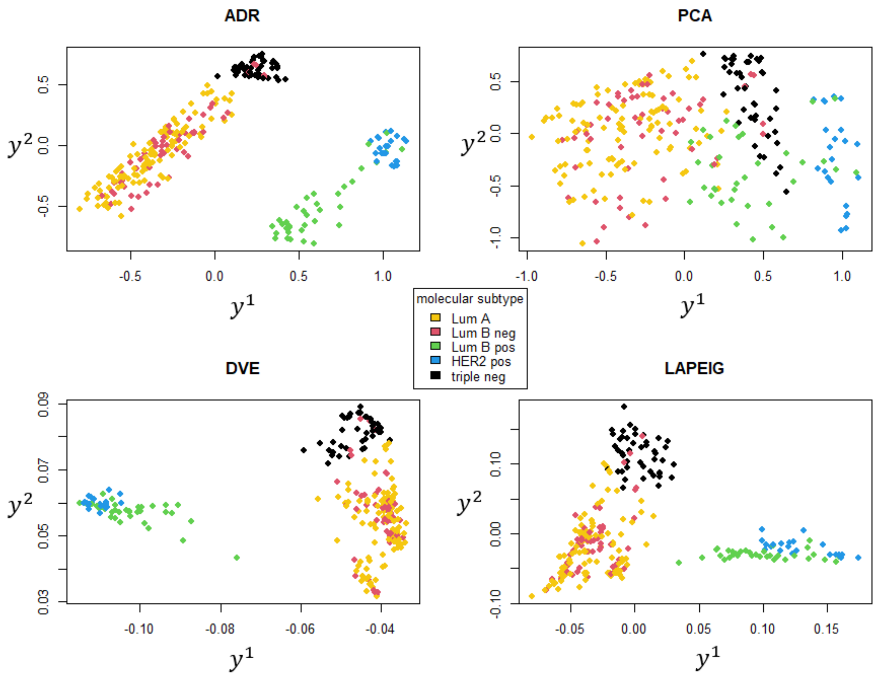
• Luminal A (ER ≥ 1% or PgR ≥ 1%, Ki67 ≤ 20%, HER2 = 0);
• Luminal B HER2 negative (ER ≥ 1% or PgR ≥ 1%, Ki67 > 20%, HER2 = 0);
• Luminal B HER2 positive (ER ≥ 1% or PgR ≥ 1%, HER2 = 1);
• HER2 positive (ER = 0% and PgR = 0%, HER2 = 1);
• Triple negative (ER = 0% and PgR = 0%, HER2 = 0).

A summary concerning therapies assigned to each molecular subtype in our data set is described in

Table 2. Correspondence between molecular subtypes and a subset of possible therapies combinations in the data set.

Molecular Subtype	HT (%)	CT (%)	CT + HT (%)	CT + Trast. (%)	CT + HT + Trast. (%)	Others (%)
Luminal A	47.3	1.8	48.2	0	1.8	0.9
Luminal B HER2 neg	30.9	12.7	54.6	0	1.8	0
Luminal B HER2 pos	5.7	2.9	25.7	0	65.7	0
HER2 pos	0	31.8	0	59.1	4.6	4.6
Triple neg	0	82.2	2.2	6.7	0	8.9

. The retrospective observational study was approved by our Institute Scientific Board.

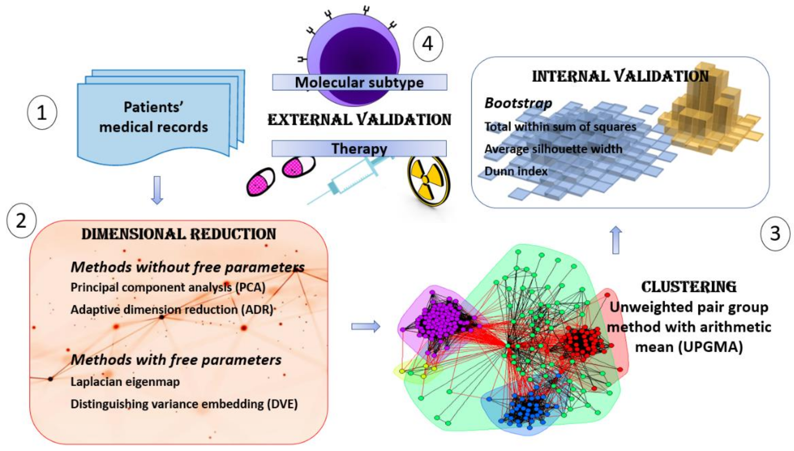
2.2. An XAI Framework for Patients’ Profiling

In this work, we propose an explainable artificial intelligence framework to evaluate which are the clinical features best representing oncological patients and capturing their similarities. A schematic overview is presented in the following Figure 1.

Thus, the proposed framework consists of four distinct steps, which are designed according to the four XAI pillars of transparency, justification, informativeness and uncertainty estimation:

• Collection of patients’ records, subject to a features processing which excludes those endowed with missing data.
• Dimensional reduction analysis, reducing the data dimensionality in a suitable two-dimensional space (for XAI transparency) and evaluating which are the clinical features driving the embedding (prodromal for XAI justification).
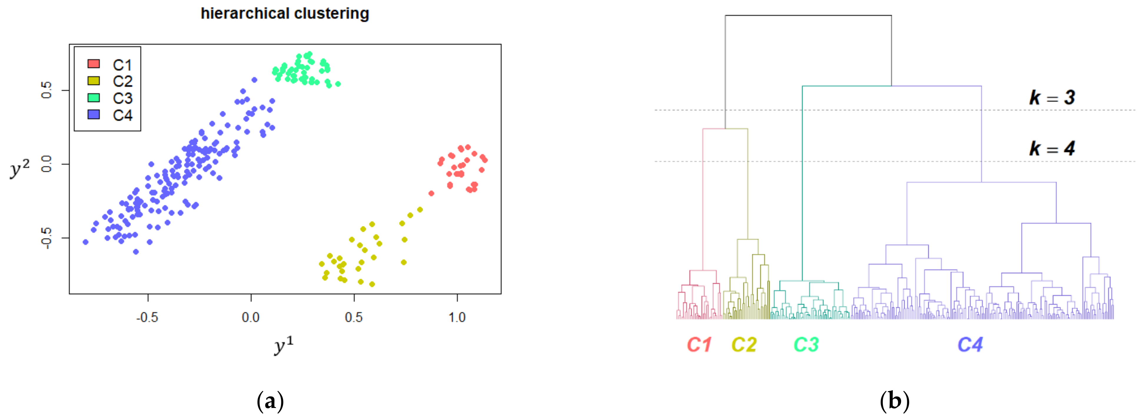
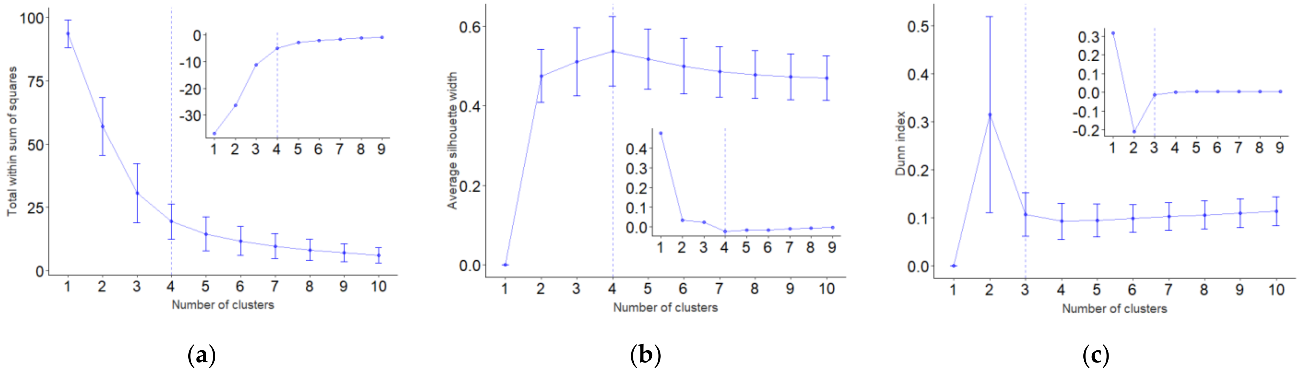
• Clustering analysis, exploring and assessing the patients’ similarities according to clinical features unveiled by embedding and bootstrap for robustness evaluation (for XAI justification and uncertainty estimation).
• Clinical and Therapy interpretation, evaluating how and to what extent the features and the clusterization previously outlined have a direct interpretation in terms of therapy differences (for XAI justification).

2.3. Dimensional Reduction Techniques

The first step of our analysis consists in the dimensional reduction. A wide variety of methods has been proposed to highlight the degrees of freedom of a data set endowed with most of the informative content. Such kinds of techniques are generally named embedding or dimensional reduction techniques; they are usually intended to project data into a subspace with a lower dimensionality to ease the data exploration, for example with the support of visual inspection or emphasize the informative content by improving the signal-to-noise-ratio. Several techniques have been proposed in the last two decades. In particular, we consider, here, the adaptive dimension reduction (ADR) approach [13].

ADR is a methodology iteratively combining the calculation of principal components and the application of k-means clustering. The motivation underlying the choice is based on a specific advantage of ADR over other effective possibilities: the absence of any parameter ruling the number of neighbors defining a local patch with respect to other popular choices such as Laplacian eigenmap [16] and distinguishing variance embedding [17,18]. Besides, ADR presents two important characteristics:

• on the one hand, the application of a principal component analysis (PCA) takes into account the information contained in the whole data set;
• on the other hand, the definition of clusters during each iteration rules further projections in the subspace spanned by principal components of the covariance matrix of cluster centers coordinates, weighted by the cardinality of each cluster, whose separation is improved.

Thus, this embedding technique perfectly matches the purposes of this work. Besides, to evaluate the robustness of the analysis, we considered other embedding techniques and compared their results with those obtained by ADR. ADR adopts PCA as a first step, followed by $k$-means clustering for the patients’ sample embedded in the space with a reduced number of dimensions. In the latter each patient is associated with a position vector ${\mathit{y}}_i$ with $1\le i\le M$ and included in a cluster $C_l$ with $1\le l\le k$, whose centroid reads

$${\mathbf{\mu }}_l=\frac{1}{\left|C_l\right|} {\displaystyle \sum }_{i \epsilon C_l}{\mathit{y}}_i$$

where $\left|C_l\right|$ stands for the number of patients in the cluster or equivalently its cardinality. This partitioning procedure is ruled by the cost function.

$$E={\displaystyle \sum }_{l=1}^k\left|C_l\right| {\displaystyle \sum }_{i \epsilon C_l}d{({\mathit{y}}_i,{\mathbf{\mu }}_l)}^2$$

which is the sum of the squared Euclidean distances between the objects $y_i$ and their centroids. It has to be minimized with respect to centroids coordinates, while the number of clusters represents a fixed parameter [22].

Once cluster memberships in the embedded space are defined, they are exploited in the original feature space, where the associated centroids coordinates define a new covariance matrix, whose PCA represents the starting of the next iterative embedding. The algorithm pursues this flowchart until it reaches a convergence to a stable configuration of embedded patients. Such iterations evaluate patients’ similarities defining clusters in the reduced dimensions space. This partition is then induced in the original space with full dimensions to define a new embedding, where another clustering is implemented until memberships are not modified in successive steps.

For further comparison and to assess the robustness of ADR results we considered embedding techniques which for their popularity can be considered the state of the art: PCA, Laplacian eigenmap and distinguishing variance embedding (DVE).

PCA represents a minimal implementation of an embedding map. The term minimal is referred to the number of operations required by the procedure: considering the diagonalization of a covariance matrix, followed by a projection onto the subspace spanned by the eigenvectors endowed with the largest eigenvalues, PCA allows the representation of high dimensional data in suitable low dimensional spaces. Importantly, such eigenvalues provide a measure of the variance explained along the directions associated with aforementioned eigenvectors, therefore they provide a tool to evaluate the informative content of the examined data.

We also considered two methods characterized according to a different approach, because they consider local patches, built as neighborhood graphs associated with each patient. Indeed, once a neighborhood is defined in the feature space in terms of a certain number of patients endowed with lowest distance with respect to a reference one, or those included into a (hyper-)sphere centered in the latter, it is possible to build an adjacency matrix. Each not vanishing entry of the adjacency matrix is then endowed with a gaussian weight

$$W_{ij}=e^{-\frac{d{\left(x_i,x_j\right)}^2}{{\sigma }^2}}$$

where $x_i$ is a scaled patient’s features vector with each component in the unit interval range and $\sigma$ is a scale parameter.

Embedded coordinates have to satisfy the same neighborhood information, as made by minimization of the cost function

$$E={\displaystyle \sum }_{i,j}d{\left({\mathit{y}}_i,{\mathit{y}}_j\right)}^2 W_{ij}$$

subject to the constraint ${{\displaystyle \sum }}_{i}d{\left({\mathit{y}}_i,0\right)}^2{D}_{ii}=1$ and $D_{ii}={\displaystyle \sum }_j{W}_{ij}$, to remove an arbitrary scaling factor to avoid the optimization lying in a subspace with less dimensions. The cost function may be expressed compactly as $E=2 Tr\left(Y^{T}L Y\right)$, where $Y$ is a $M\times n$ matrix with an embedded patient ${\mathit{y}}_i$ in each row, $Tr$ stands for the trace of a matrix and $L=D-W$ is the Laplacian matrix associated with the weighted graph, causing the name Laplacian eigenmap for the algorithm.

This optimization is also maintained in DVE, but in this case the global information of the data set is still included. A complementary graph is introduced according to the adjacency matrix $W\prime$, with unit elements between patients not considered as neighbors in the Laplacian eigenmap roadmap. In this way a further cost is evaluated in parallel

$$E\prime ={\displaystyle \sum }_{i,j}d{\left({\mathit{y}}_i,{\mathit{y}}_j\right)}^2 W{\prime }_{ij}$$

targeting its maximization to keep distant patients far apart. The embedding techniques adopted here were implemented using the open-source R (version 4.0.3) with the package Rdimtools (version 1.0.4). Further algorithmic and implementation details are provided in Appendix A and Appendix B.

2.4. Unsupervised Clustering and Validation

The dimensional reduction analysis provides a set of restricted dimensions which can suitably model the subjects’ heterogeneity. Using these dimensions and the related clinical features, we adopt a clustering procedure to characterize the similarity of the patients enrolled in this study. To this aim, we evaluated the pairwise distances between the patients in the embedding space. Then, we used the unweighted pair group method with arithmetic mean (UPGMA) [23] to build a dendrogram. This procedure combines iteratively patients in groups according to growing distance scales among them, as defined by

$$d_{A,B}=\frac{1}{\left|A\right|\left|B\right|}{{\displaystyle \sum }}_{x\epsilon A}{{\displaystyle \sum }}_{y\epsilon B}d\left(x,y\right)$$

followed by the next patients’ group distance weighted by the cardinality of the previous groups $d_{A\cup B,C}=\left(\left|A\right|d_{A,C}+\left|B\right|d_{B,C}\right)/\left(\left|A\right|+\left|B\right|\right)$. In this way we define communities of patients typical of each distance scale. The distance is computed by considering the feature in a Euclidean reference system. The choice of the cutting level in the dendrogram is implemented according to internal validations, which reward cluster compactness and separation, while to measure how much the yielded partition matches with the studied medical variables we used the external validation. In particular, the decision tree nature of molecular subtypes allows us to improve explainability [10]. To evaluate the robustness of the cluster analysis, several metrics were investigated, such as total within sum of squares, average silhouette width, Dunn index and adjusted Rand index [22,24,25] (Appendix C). The limited cardinality of the considered data set imposes a required quantification of uncertainty that we implement by means of a bootstrap procedure [26]. Bootstrap consists in sampling data with replacement in order to obtain replica of the original data which statistically follow the same distribution. To ensure a higher fidelity of this procedure, we replicate the original data set by adopting a sampling ratio equal to the 80% of the available instances. This ratio ensures that the balance of considered labels is preserved. This procedure is implemented 1000 times, in each trial evaluating the three internal validations and the ARI external validation for both molecular subtypes and therapy labels. Internal and external validation metrics were implemented by means of R packages Clustering (version 1.7.2), factoextra (version 1.0.7) and mclust (version 5.4.7).

3. Results

3.1. Comparing the Embedding Techniques

Our targeted roadmap towards a XAI being able to identify optimal therapy schemes has to rely on the detection of most informative variables in this purpose, whose role can be verified by the procedure adopted in current guidelines. First of all, we evaluated the different embedding techniques and compared their output using $n=2$ dimensions, as shown in Figure 2.

The color legend shows the molecular subtype of the patient’s tumor. Interestingly, the two-dimensional embedding shows a cluster structure. Clusters seem to reproduce the molecular subtype, a property slightly affected by the embedding technique, but ADR emphasizes the separation of each group.

To evaluate the informative content of such clusters and to obtain an interpretation, we considered which features most influence this representation. Focusing on the ADR technique, which resulted in the clearest representation, we evaluated the most important eigenvectors and examined their components: ER, PgR, Ki67 and HER2 resulted as the most significant ones. We underline that these features are exactly those defining the molecular subtypes, according to the associated decisional trees, whose selection in the relevant space appears to be an important result from a clinical point of view. By construction, the sum of squared coefficients of vectors spanning the relevant space equals to one, so we express the aforementioned weights in terms of percentages assumed by the square coefficient associated with each initial feature. The first principal component in output of the ADR procedure assigns to ER a squared coefficient equal to 20.9%, 16.1% to PgR, 2.8% to Ki67 and 56.7% to HER2. Globally, these initial features cover 96.5% of the overall unitary sum of squared coefficients. The second ADR component allocates to ER 37.5%, to PgR 18.8%, to Ki67 1.8% and to HER2 39.2%, now totally covering 97.3%, that is quite the overall variability.

We chose some well-established dimensional reduction procedures to underline the robustness of the selected information once the same characterization is approximately observed in the output of each technique. The PCA embedding yields molecular subtype groups with a low separation with respect to remaining methods, because of the very simple structure of the associated algorithm. Nevertheless, it is possible already to underline the common indistinguishability shared by all embedding techniques between Luminal A and Luminal B HER2 negative patients. ADR, Laplacian eigenmap and DVE show much more separated HER2 positive and Luminal B HER2 positive patients, as well as triple negative cases. The absence for free parameters other than the embedded space dimension gives to ADR a privileged role for our purposes. Indeed, both Laplacian eigenmap and DVE are based on local patches defined through a parameter associated with the number of neighbors for each patient. In Figure 2 both cases adopt this number equal to 15 to maximize the cluster separation, even if it is data set dependent, because a different number of members is associated with each molecular subtype and patches should match as much as possible with this membership limitation.

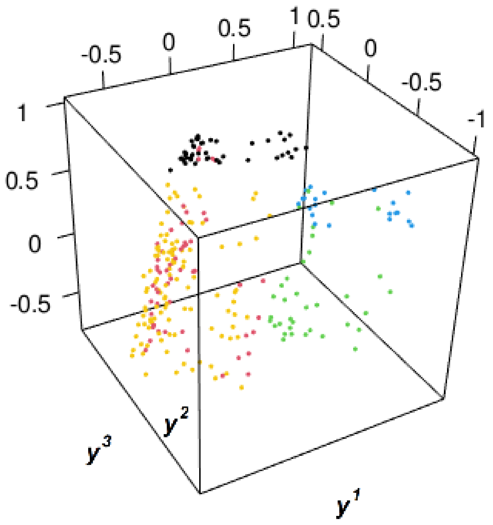
3.2. Clustering Oncological Patients

The UPGMA clustering of the ADR embedding is described in Figure 3, where we highlight its hierarchical structure established according to the dendrogram. This latter is characterized by the definition of patients’ communities typical of each distance level corresponding to which we apply a cut. This action selects the information expressed by a certain distance scale, thus grouping the elements accordingly. Our unsupervised procedure aims at the detection of molecular subtype and consequently of therapy information by cutting the dendrogram at the appropriate level.

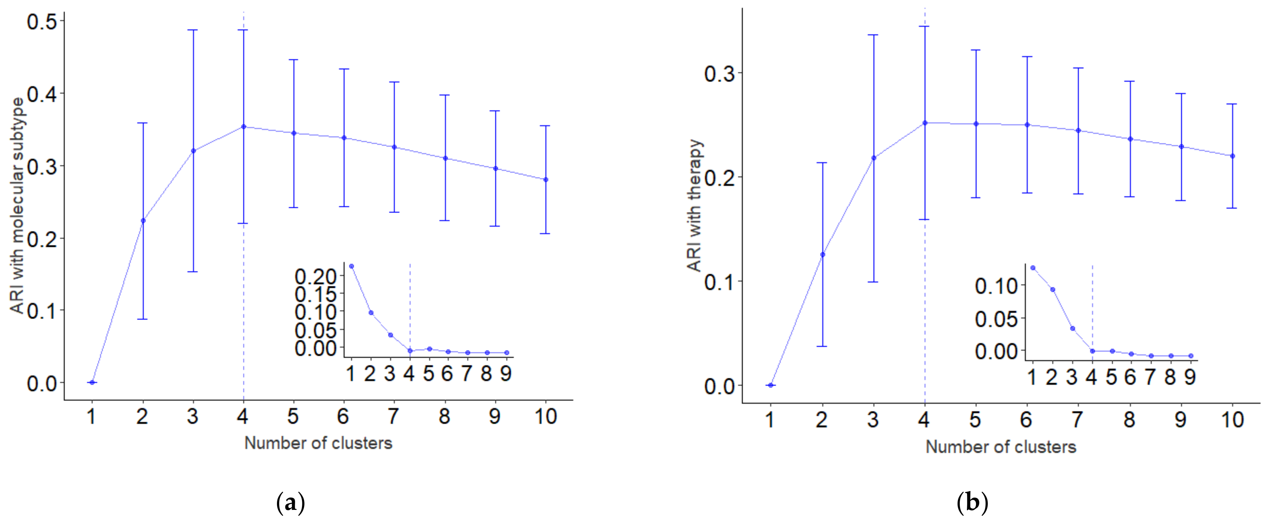
3.2.1. Internal Validation

The selection of an optimal number of clusters is ruled by internal validation methods. The behavior of these quantities with respect to the number of clusters $k$ is depicted in Figure 4 and it allows us to identify some optimal conditions. We choose to support the selection of the optimal condition by adding the information contained in the interquartile range provided by a bootstrap procedure replicating a subsample with the 80% of the original sample cardinality, together with the first derivative of each mean index, intended as a function of the number of clusters, shown in the inbox of each plot in Figure 4. Indeed, according to the presented criteria $k=4$ is the choice suggested by $WSS$ function, while by observing just the silhouette index we may follow the maximal variation obtained with lowest $k$ value, thus leading to $k=2$. The function $w$ averaged over all patients reaches its maximum value corresponding to $k=4$, so it represents a confirmation of the optimal number given by the total within sum of squares. Instead, Dunn index suggested to cut the dendrogram in Figure 3 corresponding to $k=3$ clusters, so grouping toghether HER2 positive and Luminal B HER2 positive patients. These molecular subtypes present a similar clinical behavior caused by the correlated higher values for Ki67 with HER2 positivity.

3.2.2. External Validation

In our data set 110 patients belong to the luminal A subtype, 55 are in the luminal B HER2 negative condition, 35 in luminal B HER2 positive, 22 in HER2 positive and 45 in triple negative. Once a category among the latter is chosen for a patient, a therapy is assigned by clinicians to each case according to characterizing specificities and the presence of possible comorbidities. We resume the therapy statistics characterizing each molecular subtype in Table 2.

Results presented in

Table 3. Correspondence between clusters and molecular subtypes in the data set.

Cluster	Luminal A (%)	Luminal B HER2 Neg (%)	Luminal B HER2 Pos (%)	HER2 Pos (%)	Triple Neg (%)
C1	0	0	21.4	78.6	0
C2	0	0	100.0	0	0
C3	0	10.2	0	0	89.8
C4	68.3	31.1	0	0	0.6

highlight misclassifications of patients belonging to luminal B HER2 negative and positive subtypes, corresponding numerically to five and six cases included among triple negative and HER2 positive molecular subtypes, respectively. The wrong inclusion is explained by considering the mean value of biomarkers for hormonal receptors, that in the cluster C4 read $〈\mathrm{ER}〉=65.3$ and $〈\mathrm{PgR}〉=50.1$, while for misclassified patients in C3 read $〈\mathrm{ER}〉=0.4$ and $〈\mathrm{PgR}〉=4.8$ and $〈\mathrm{Ki}67〉=20.6$, so signaling a much lower value for the hormonal receptors expression. Analogously in C2 we observe $〈\mathrm{ER}〉=61.5$ and $〈\mathrm{PgR}〉=34.4$, while misclassifications in C1 are endowed with $〈\mathrm{ER}〉=5.2$ and $〈\mathrm{PgR}〉=7.7$.

To quantify the correspondence between clusters and molecular subtype or therapy labels, we evaluate ARI for both cases. To establish a baseline this calculation is implemented in the variation of the number of clusters $k$: the behavior of the index is shown in Figure 5, where we highlight the confirmation for the choice of optimal number of clusters, because the maximum value is reached corresponding to $k=4$ in both cases. Moreover, approximately the same derivative characterizes both plots, thus strengthening the relation between therapies and molecular subtypes in a completely unsupervised way.

The clusters yielded by UPGMA contain a prevalent group in terms of both molecular subtypes or therapies, as resumed in Table 3. The maximal number of cluster members with respect to therapy correspond to the one observed in Table 2.

4. Discussion

Biomarkers are currently widely exploited in computer-aided diagnosis (CAD) tools in case of complex diseases such as cancer, intrinsically requiring a multifactorial study, as made for the prediction of optimal chemotherapeutic plans by fusing their information content with genic expressions [27], thus supporting the maintenance of a privileged role for cancer cell receptors in our XAI perspective towards therapy assignment.

XAI applications with medical purposes are increasingly widespread [28,29], based on the fundamental achievement of interpretability, which represents the main difference with brute force deep learning approaches. In particular, the exploitation of these algorithmic schemes for breast cancer is currently adopted for classification of malignant cases, as well as recurrent ones. With this aim the multidimensional scaling is implemented to obtain embedding in a relevant space, followed by a different step with respect to our flowchart, represented by rainbow boxes [29], which may be exploited in further developments targeting the use of query patients. In literature, a clustering technique analogous to the one presented in this study with UPGMA is used in the definition of symptoms groups among cancer patients, based on the purpose to provide a support in the definition of therapies [30,31]. Interestingly, the main objective is already focused on a robust patients’ stratification by using ensemble clustering [31], thus partly anticipating the current application of XAI in medical purposes.

The output of our XAI procedure [9] satisfies transparency, because it is strictly linked with the complete knowledge of the flowchart depicted in Figure 1. Justification is supported by a cross evaluation of the emergent effective feature consisting in the molecular subtype with the therapy label, which is the target of XAI for medical purposes. Uncertainty estimations are sketched with the help of bootstrap, while the missing informativeness at this stage will be tested in future developments according to the employment of new data sources. Indeed, a higher number of features can be retained as endowed with an information content if the used bioinformatics data are correlated with the ones yielded by different sources: this data integration will be targeted in further investigations addressing the indistinguishability of Luminal A and Luminal B HER2 negative subtypes observed for any embedding technique in Figure 2 and residing in the small weight attributed to the Ki67 biomarker.

Nevertheless, the clustering depicted in Figure 3 shows an accurate selection of molecular subtypes, as proved in Table 3, while a less precise selection of therapies is described in

Table 4. Correspondence between clusters and a subset of possible therapies combinations in the data set.

Cluster	HT (%)	CT (%)	CT + HT (%)	CT + Trast. (%)	CT + HT + Trast. (%)	Others (%)
C1	0	25.0	3.6	46.4	21.4	3.6
C2	6.9	3.4	27.6	0	62.1	0
C3	0	85.7	2.0	6.1	0	6.1
C4	42.9	2.4	51.6	0	1.9	1.2

, probably caused by not included factors characterizing each patient, as well as associated comorbidities. The bootstrap test of the presented clusters, reaching an ARI approximately equal to 0.6 with respect to molecular subtypes and 0.4 with therapies, reveals a lower level of performances, as represented in Figure 5 where the lower values assumed by ARI with therapies labels are still observed.

Concerning the selection of the optimal number of clusters described in Figure 4, we have to stress that the presented results are preliminary and included in a more general framework referred to personalized medicine. Furthermore, the cardinality of our data set does not allow us to configure the discussion in the high dimensional setting. This characterization translates into internal validation indices not endowed with a stable behavior with respect to the variation in the number of clusters, which motivated our choice for a bootstrap procedure, as well as to take into account the optimal number of cluster once the first derivative associated with mean indices establishes a steady condition. The selection of $k=4$ is supported both in a supervised way by ARI and in an unsupervised one by the total within sum of squares and the average silhouette width, even if taking into account error bars $k=3$ represents an equivalent choice, which is suggested by the Dunn index. According to the therapeutic perspective this equivalence is motivated by the similar clinical characterization of Luminal B HER2 positive and HER2 positive subtypes, because the correlation of high values for Ki67 with HER2 positivity induces a widespread adoption of chemotherapy. It is important to underline that the maximum value of the Dunn index together with the most pronounced variation of the average silhouette width are associated with $k=2$, so related with just the HER2 discrimination.

Results shown in Table 4 matching the most frequent therapeutic plan observed in Table 2 establish that misclassifications regarding subtypes do not prefer a certain therapeutic strategy, but they spread over all combinations, thus maintaining the same prevalent assignment given by clinicians per subtype. Moreover, the behavior of ARI curves represented in Figure 5 is equivalent, unless regarding the values they reach, thus confirming that the overall trend is well captured by our clustering procedure and therapy inaccurate assignments implemented by clustering are just statistical fluctuations. The correspondence between molecular subtypes and therapies shown in Table 2 represents the hinge of our unsupervised clustering procedure with health care plans assigned by clinicians to each patient.

5. Conclusions

In this work we present results concerning an unsupervised definition of clusters of breast cancer patients diagnosed with a first tumor. The adaptive dimension reduction method is combined with the average distance clustering, whose output is compared with molecular subtype and therapy labels through the adjusted rand index metric. Internal validation indices show the limits of our study linked with the small cardinality of the data set, thus characterizing it as a preliminary analysis inserted in the more general personalized medicine purpose. The equivalent behavior of the unsupervised partition with respect to both labeling ensures the robustness of the clinical decision, here considered just as a label, so not included as a feature.

Besides, this result guarantees further developments of the implemented procedure to detect therapy information in an unsupervised way among elements of unstructured datasets, as well as to suggest modification in therapeutic plans. In this perspective once a sufficiently populated database is obtained, we may think to implement a query of new patients subject to a case-based reasoning able to detect specificities and comorbidities, as well as to improve tumor recurrences by adopting a most suitable therapeutic scheme.

References

1. Hulsen, T.; Jamuar, S.S.; Moody, A.R.; Karnes, J.H.; Varga, O.; Hedensted, S.; Spreafico, R.; Hafler, D.A.; McKinney, E.F. From Big Data to Precision Medicine. Front. Med. 2019, 6, 34. [Google Scholar] [CrossRef] [Green Version]
2. Avanzo, M.; Trianni, A.; Botta, F.; Talamonti, C.; Stasi, M.; Iori, M. Artificial Intelligence and the Medical Physicist: Welcome to the Machine. Appl. Sci. 2021, 11, 1691. [Google Scholar] [CrossRef]
3. Syeda-Mahmood, T. Role of Big Data and Machine Learning in Diagnostic Decision Support in Radiology. J. Am. Coll. Radiol. 2018, 15, 569–576. [Google Scholar] [CrossRef] [PubMed]
4. Arabi, H.; Zaidi, H. Applications of artificial intelligence and deep learning in molecular imaging and radiotherapy. Eur. J. Hybrid Imaging 2020, 4, 17. [Google Scholar] [CrossRef]
5. Avanzo, M.; Porzio, M.; Lorenzon, L.; Milan, L.; Sghedoni, R.; Russo, G.; Massafra, R.; Fanizzi, A.; Barucci, A.; Ardu, V.; et al. Artificial intelligence applications in medical imaging: A review of the medical physics research in Italy. Phys. Med. 2021, 83, 221–241. [Google Scholar] [CrossRef]
6. Massafra, R.; Latorre, A.; Fanizzi, A.; Bellotti, R.; Didonna, V.; Giotta, F.; La Forgia, D.; Nardone, A.; Pastena, M.; Ressa, C.M.; et al. A Clinical Decision Support System for Predicting Invasive Breast Cancer Recurrence: Preliminary Results. Front. Oncol. 2021, 11, 1–13. [Google Scholar] [CrossRef]
7. Fanizzi, A.; Pomarico, D.; Paradiso, A.; Bove, S.; Diotaiuti, S.; Didonna, V.; Giotta, F.; La Forgia, D.; Latorre, A.; Pastena, M.I.; et al. Predicting of Sentinel Lymph Node Status in Breast Cancer Patients with Clinically Negative Nodes: A Validation Study. Cancers 2021, 13, 352. [Google Scholar] [CrossRef]
8. Pomarico, D.; Fanizzi, A.; Amoroso, N.; Bellotti, R.; Biafora, A.; Bove, S.; Didonna, V.; La Forgia, D.; Pastena, M.I.; Tamborra, P.; et al. A proposal of quantum-inspired machine learning for medical purposes: An application case. Mathematics 2021, 9, 410. [Google Scholar] [CrossRef]
9. Jiménez-Luna, J.; Grisoni, F.; Schneider, G. Drug discovery with explainable artificial intelligence. Nat. Mach. Intell. 2020, 2, 573–584. [Google Scholar] [CrossRef]
10. Gunning, D. Explainable Artificial Intelligence (XAI); Defense Advanced Research Projects Agency (DARPA): Arlington, VA, USA, 2017; Web 2.2. [Google Scholar]
11. Došilović, F.K.; Brčić, M.; Hlupić, N. Explainable artificial intelligence: A survey. In Proceedings of the 2018 41st International Convention on Information and Communication Technology, Electronics and Microelectronics (MIPRO), Opatija, Croatia, 21–25 May 2018. [Google Scholar]
12. Coates, A.S.; Winer, E.P.; Goldhirsch, A.; Gelber, R.D.; Gnant, M.; Piccart-Gebhart, M.; Thürlilmann, B.; Senn, H.-J.; André, F.; Baselga, J.; et al. Tailoring therapies—Improving the management of early breast cancer: St Gallen International Expert Consensus on the Primary Therapy of Early Breast Cancer. Ann. Oncol. 2015, 26, 1533–1546. [Google Scholar] [CrossRef] [PubMed]
13. Ding, C.; He, X.; Zha, H.; Simon, H.D. Adaptive dimension reduction for clustering high dimensional data. In Proceedings of the 2002 IEEE International Conference on Data Mining, Maebashi City, Japan, 9–12 December 2002. [Google Scholar]
14. Hotelling, H. Analysis of a complex of statistical variables into principal components. J. Educ. Psychol. 1933, 24, 417–441, 498–520. [Google Scholar] [CrossRef]
15. Kutz, J.N. Data-Driven Modeling & Scientific Computation: Methods for Complex Systems & Big Data; Oxford University Press: Oxford, UK, 2013. [Google Scholar]
16. Belkin, M.; Niyogi, P. Laplacian eigenmap for dimensionality reduction and data representation. Neural Comput. 2003, 15, 1373–1396. [Google Scholar] [CrossRef] [Green Version]
17. Qinggang, W.; Jianwei, L. Combining local and global information for nonlinear dimensionality reduction. Neurocomputing 2009, 72, 2235–2241. [Google Scholar]
18. Qinggang, W.; Jianwei, L.; Xuchu, W. Distinguishing variance embedding. Image Vis. Comput. 2010, 28, 872–880. [Google Scholar] [CrossRef]
19. Duffy, M.J.; Crown, J. A personalized approach to cancer treatment: How biomarkers can help. Clin. Chem. 2008, 54, 1770–1779. [Google Scholar] [CrossRef] [PubMed] [Green Version]
20. Rivenbark, A.G.; O’Connor, S.M.; Coleman, W.B. Molecular and cellular heterogeneity in breast cancer: Challenges for personalized medicine. Am. J. Pathol. 2013, 183, 1113–1124. [Google Scholar] [CrossRef] [Green Version]
21. Tannock, I.F.; Hickman, J.A. Limits to personalized cancer medicine. N. Engl. J. Med. 2016, 375, 1289–1294. [Google Scholar] [CrossRef] [Green Version]
22. Amoroso, N.; Cilli, R.; Bellantuono, L.; Massimi, V.; Monaco, A.; Nitti, D.O.; Nutricato, R.; Samarelli, S.; Taggio, N.; Tangaro, S.; et al. PSI Clustering for the Assessment of Underground Infrastructure Deterioration. Remote Sens. 2020, 12, 3681. [Google Scholar] [CrossRef]
23. Sokal, R.B.; Michener, C.D. A statistical method for evaluating systematic relationships. Univ. Kans. Sci. Bull. 1958, 38, 1409–1438. [Google Scholar]
24. Hubert, L.; Arabie, P. Comparing partitions. J. Classif. 1985, 2, 193–218. [Google Scholar] [CrossRef]
25. Pérez, L.A.; García Vico, A.M.; González, P.; Carmona, C.J. Techniques for Evaluating Clustering Data in R. The Clustering package 2020. [Google Scholar]
26. Efron, B.; Tibshirani, R. An Introduction to the Bootstrap; Chapman & Hall/CRC: Boca Raton, FL, USA, 1993. [Google Scholar]
27. Kim, Y.Y.; Oh, S.J.; Chun, Y.S.; Lee, W.K.; Park, H.K. Gene expression assay and Watson for Oncology for optimization of treatment in ER-positive, HER2-negative breast cancer. PLoS ONE 2018, 13, e0200100. [Google Scholar] [CrossRef] [PubMed]
28. Tjoa, E.; Guan, C. A Survey on Explainable Artificial Intelligence (XAI): Toward Medical XAI. IEEE Trans. Neural Netw. Learn. Syst. 2020. [Google Scholar] [CrossRef]
29. Lamy, J.-B.; Sekar, B.; Guezennec, G.; Bouaud, J.; Séroussi, B. Explainable artificial intelligence for breast cancer: A visual case-based reasoning approach. Artif. Intell. Med. 2019, 94, 42–53. [Google Scholar] [CrossRef] [PubMed]
30. Walsh, D.; Rybicki, L. Symptom clustering in advanced cancer. Support Care Cancer 2006, 14, 831–836. [Google Scholar] [CrossRef]
31. Chen, D.; Xing, K.; Henson, D.; Sheng, L.; Schwartz, A.M.; Cheng, X. Developing Prognostic Systems of Cancer Patients by Ensemble Clustering. J. Biomed. Biotech. 2009. [Google Scholar] [CrossRef] [PubMed]
Figure 1. Schematic overview of the presented flowchart, including four main phases: (1) data collection; (2) dimensional reduction; (3) clustering and (4) clinical validation. Further details about these steps are presented in the text.
Applsci 11 04881 g001
Figure 2. Two-dimensional projection of original data in the plane spanned by relevant degrees of freedom y = y 1 , y 2 . DVE and LAPEIG (Laplacian eigenmap) are implemented using 15 patients as neighbors composing each local patch.
Applsci 11 04881 g002
Figure 3. Hierarchical clustering yielded by UPGMA for the ADR embedding in panel (a), ruled by the associated dendrogram in panel (b) where two possible cutting level are highlighted.
Applsci 11 04881 g003
Figure 4. Representation of internal validation methods adopted for the selection of the optimal number of clusters: panel (a) corresponds to the function W S S k , average of the silhouette width is shown in panel (b) and Dunn index is associated with panel (c). The inbox describes the finite differences derivative referred to the mean blue line lying in the interquartile range shown according to error bars provided by bootstrap.
Applsci 11 04881 g004
Figure 5. Dependence of ARI on the number of clusters, which is computed with respect to the correspondence between the unsupervised clustering and molecular subtypes in (a) and therapy combinations in (b). The blue line joins mean values included in the error bars and associated with the interquartile range yielded by bootstrap, whose finite difference derivative is described in the inbox.
Applsci 11 04881 g005