Learning the Parametric Transfer Function of Unitary Operations for Real-Time Evaluation of Manufacturing Processes Involving Operations Sequencing

Featured Application

This paper aims at proposing a machine learning methodology for creating a parametric transfer function of unitary operations, to be applied in the real-time evaluation of sequenced operations. This methodology will be applied to the real-time evaluation of induced structural distortions when printing stiffeners, for any chosen printing operation sequencing.

Abstract

For better designing manufacturing processes, surrogate models were widely considered in the past, where the effect of different material and process parameters was considered from the use of a parametric solution. The last contains the solution of the model describing the system under study, for any choice of the selected parameters. These surrogate models, also known as meta-models, virtual charts or computational vademecum, in the context of model order reduction, were successfully employed in a variety of industrial applications. However, they remain confronted to a major difficulty when the number of parameters grows exponentially. Thus, processes involving trajectories or sequencing entail a combinatorial exposition (curse of dimensionality) not only due to the number of possible combinations, but due to the number of parameters needed to describe the process. The present paper proposes a promising route for circumventing, or at least alleviating that difficulty. The proposed technique consists of a parametric transfer function that, as soon as it is learned, allows for, from a given state, inferring the new state after the application of a unitary operation, defined as a step in the sequenced process. Thus, any sequencing can be evaluated almost in real time by chaining that unitary transfer function, whose output becomes the input of the next operation. The benefits and potential of such a technique are illustrated on a problem of industrial relevance, the one concerning the induced deformation on a structural part when printing on it a series of stiffeners.

1. Introduction

When joining one flexible part to another with several screw holes, it is not uncommon to end with some screws that do not enter in their hole. This can be due to some tolerance issue, but it can also be due to the deformation of the part induced by the residual stresses due to the stresses applied by the previous operations. In this case, the parts can not be successfully joined because of the order chosen in the joining unitary operations, as illustrated with the red screw in Figure 1.

In the industry, this example from everyday life is often met when welding [1,2,3], screwing, or joining two flexible parts: if the operations of fixation are not executed in a well designed order, these parts may not be well assembled considering the project requirements. Additive manufacturing of stiffeners on metal sheets produces the same kind of issues [4,5]. It generates some deflections on these parts. This results in an impossibility to assemble them on the whole structure.

To design this kind of sequential processes, one possible solution is to test some specific sequences which seem suitable in high fidelity simulations. Indeed, for sequences involving a lot of unitary operations, it is not an option to compute each of them: computational time for only one sequence of operations may take several hours. Thus, teams designing these processes explore a very small area of the space of possible sequences. Thus, the quite poor exploration of the design space results in a non optimal choice of the process sequencing. Some sequences may have improved significantly the quality of the final product, but they were not tested because of the unaffordable computational time to test all possible combinations (often in the order of millions).

To overcome the computational cost issue, a valuable route consists of using a reduced order model [6,7,8]. The main purpose of model order reduction is to identify a statistical approximation function f that transforms the inputs X into outputs Y

$$Y\approx f\left(X\right).$$

(1)

Nowadays, these approaches are very common in the industry: aerodynamics, thermal comfort, Noise–Vibrations–Harshness (NVH), nonlinear transient dynamics. For a given loading, the studied system is simulated for several choices of the design parameters. Then, inputs and outputs are extracted. Finally, the Reduced Order Model –ROM– is built by computing the approximation function f. The learned model enables simulation, optimization, inverse analysis, uncertainty propagation, and simulation-based control, in almost real time, with the expected positive impact in the design and validation processes.

The use of reduced basis in support of machine learning of parametric models or dynamical systems is attracting the interest of the scientific community [9,10]. Building reduced order models –ROMs– of a series of unitary operations remains a challenging issue for the state-of-the-art methodologies because of the combinatorial explosion induced by all the possible sequences of applying those unitary operations. In this work, we propose a methodology that allows for alleviating that difficulty, where, more than looking for representing the effect of any possible sequence, we look for describing the effect of a unitary operation on the thermomechanical state resulting from the previous unitary operation. The efficient implementation is based on the fact that the thermomechanical state all along the whole process can be efficiently expressed (parametrized) in a reduced basis, extracted by invoking the Singular Values Decomposition –SVD–.

This methodology concerns both data preparation and regression. Concerning the data, a reduced basis able to represent any possible state of the system will be extracted. Its coefficients, describing the projection of any state on that basis, is assumed as features of the learned model. The other features are the ones related to the sequencing. Concerning the regression able to transform the input features (present state) into the output describing the state of the system after a unitary operation, according to the sequencing plan, two different techniques will be employed and compared: the Neural Network –NN– [11] and the Dynamic Mode Decomposition –DMD– [12].

A dictionary of unitary operations will be constructed with all the corresponding unitary transfer functions. It will then be used in order to evaluate any sequencing almost in real time, by chaining these unitary transfer functions, whose output becomes the input of the next operation.

The benefits and potential of such a technique will be illustrated on a problem of industrial relevance: the one concerning the induced deformation on a structural part when printing on it a series of stiffeners, as presented in Section 2.

2. Materials and Methods

The methodology presented in this paper has been developed on a representative case of study. In this section, we briefly revisit the techniques that will be employed. Then, we describe the case of study we used in this work. Finally, we present the whole methodology, from the model construction to the surrogate model use. In what follows, all the high fidelity simulations have been performed offline by using the commercial software VPS (Virtual Performance Solution) by ESI Group. The whole reduction process is then made by using a standard laptop (6 cores, 3 GHz, 16 GB RAM).

2.1. Data Reduction and Model Learners

For the sake of completeness, this subsection revisits the main techniques that will be employed later: the Singular Values Decomposition –SVD–, the Dynamic Mode Decomposition –DMD–, and the Multi-Layer Perceptron –MLP–.

2.1.1. Singular Values Decomposition

The purpose of the SVD [13] is to decompose any rectangular matrix A of dimensions $N\times T$ as the product of three matrices: U, $\Sigma$, and $V^{\mathrm{T}}$

$$A=U\Sigma V^{\mathrm{T}},$$

(2)

where U is an orthogonal matrix of dimension $N\times N$, $\Sigma$ a diagonal matrix and V an orthogonal matrix of dimensions $T\times T$ (here, it is assumed that all the matrices are real valued).

Columns of U are the principal components of A, also called modes. Non-zero components of $\Sigma$, ${\sigma }_1\ge {\sigma }_2\ge \cdots$, are called singular values. Columns of V are the principal components of size T instead of N: if N is the number of degrees of freedom and T the number of time instants in the dataset, columns of U are the space principal components and columns of V are the time principal components.

With this decomposition, one can easily approximate ${\mathbf{a}}_{\mathbf{i}}$, the ith column of A, by projecting it on the principal components, to compute its reduced coordinates $({\alpha }_{i1},\cdots ,{\alpha }_{ir})$

$$\left[{\alpha }_{i,1}\cdots {\alpha }_{i,r}\right]={\mathbf{a}}_{\mathbf{i}}^{\mathrm{T}}\tilde{U},$$

(3)

where $\tilde{U}$ contains the first r columns of U.

The columns ${\mathbf{a}}_{\mathbf{i}}$ can be approximated in the reduced basis composed by the columns of $\tilde{U}$

$${\mathbf{a}}_{\mathbf{i}}\approx \sum _{j=1}^r{\alpha }_{ij}{\mathbf{u}}_{\mathbf{j}}.$$

(4)

Thus, the SVD allows for approximating any rectangular matrix A by projecting its columns in a reduced basis consisting of r dimensions instead of N, with in general $N\gg r$. More details on this technique can be found in [14,15,16].

2.1.2. Dynamic Mode Decomposition

When working on the approximation of a dynamical system, one can try to reduce its complexity. One can also be tempted in approximating the state X at time $t_{i+1}$ from the one existing at time $t_i$, $\forall i$

$$X\left(t_{i+1}\right)=f\left(X\left(t_i\right)\right),i\in \{1,\dots ,T-1\}.$$

(5)

This is the rationale employed in the DMD [17,18,19,20]. Equation (5) can be rewritten as

$$X\left(t_{i+1}\right)=AX\left(t_i\right),i\in \{1,\dots ,T-1\},$$

(6)

with A a square matrix of size N. Writing Equation (6) for each state of the system leads to the following matrix equation:

$$\mathbb{X}=A\tilde{\mathbb{X}},$$

(7)

with $\mathbb{X}=\left[X_T{X}_{T-1}\cdots X_2\right]$, $\tilde{\mathbb{X}}=\left[X_{T-1}{X}_{T-2}\cdots X_1\right]$. The DMD model, i.e., the matrix A, can be computed by applying different techniques, one of them described and used later. By replacing the linear operator A with a nonlinear function f, stronger nonlinearities can be efficiently addressed as reported in [21] by using neural networks.

2.1.3. Multi-Layer Perceptron

Neural Networks are a class of nonlinear regressors. Given a set of inputs X and a set of outputs Y, one can easily use a Neural Network to compute a nonlinear function f such as

$$Y\approx f\left(X\right).$$

(8)

When an NN contains more than one hidden layer of neurons, it is called Multi-Layer Perceptron. Figure 2 schematizes the architecture of a MLP with one hidden layer consisting of p neurons. The MLP takes as inputs vectors of size n and transforms them into output vectors of size m.

In the MLP illustrated in Figure 2, coefficients ${\omega }_{i,j}$ and $h_{i,j}$ are the weights of the neurons connectors, and k refers to the $k^{th}$ data in the Design of Experiments –DoE–. The function that generates the $i^{th}$ component of an output $Y_k$ from the input $X_k$ reads

$$Y_{k,i}=f_i\left(X_k\right)=\varphi \left(\sum _{l=1}^p{h}_{l,i}\varphi \left(\sum _{j=1}^n{\omega }_{l,j}{X}_{k,j}+b_1\right)+b_2\right),$$

(9)

with $b_1$ and $b_2$ the bias introduced at each connection and $\varphi$ the activation function. The weights of $f_i$ are obtained by minimizing the difference between the output prediction and the known output that is $\parallel Y_{k,i}-f_i\left(X_k\right)\parallel$, for all $i,k$.

The trickiest concern when using the MLP is the choice of the so-called hyper-parameters, e.g., number of layers, number of neurons in the hidden layers, etc. For additional information, the interested reader can refer to [22,23,24,25].

2.2. Case of Study

In complex metallic structures, it is often required to weld some parts or to print stiffeners by using additive manufacturing to enhance mechanical performances. These kinds of operations induce structural distortions, due to the installed residual stresses.

Predicting those induced distortions allows for finding the optimal operations sequencing to minimize them, or to design a modified structure such that the induced distortions will produce the wished final structure geometry fulfilling the requested tolerances.

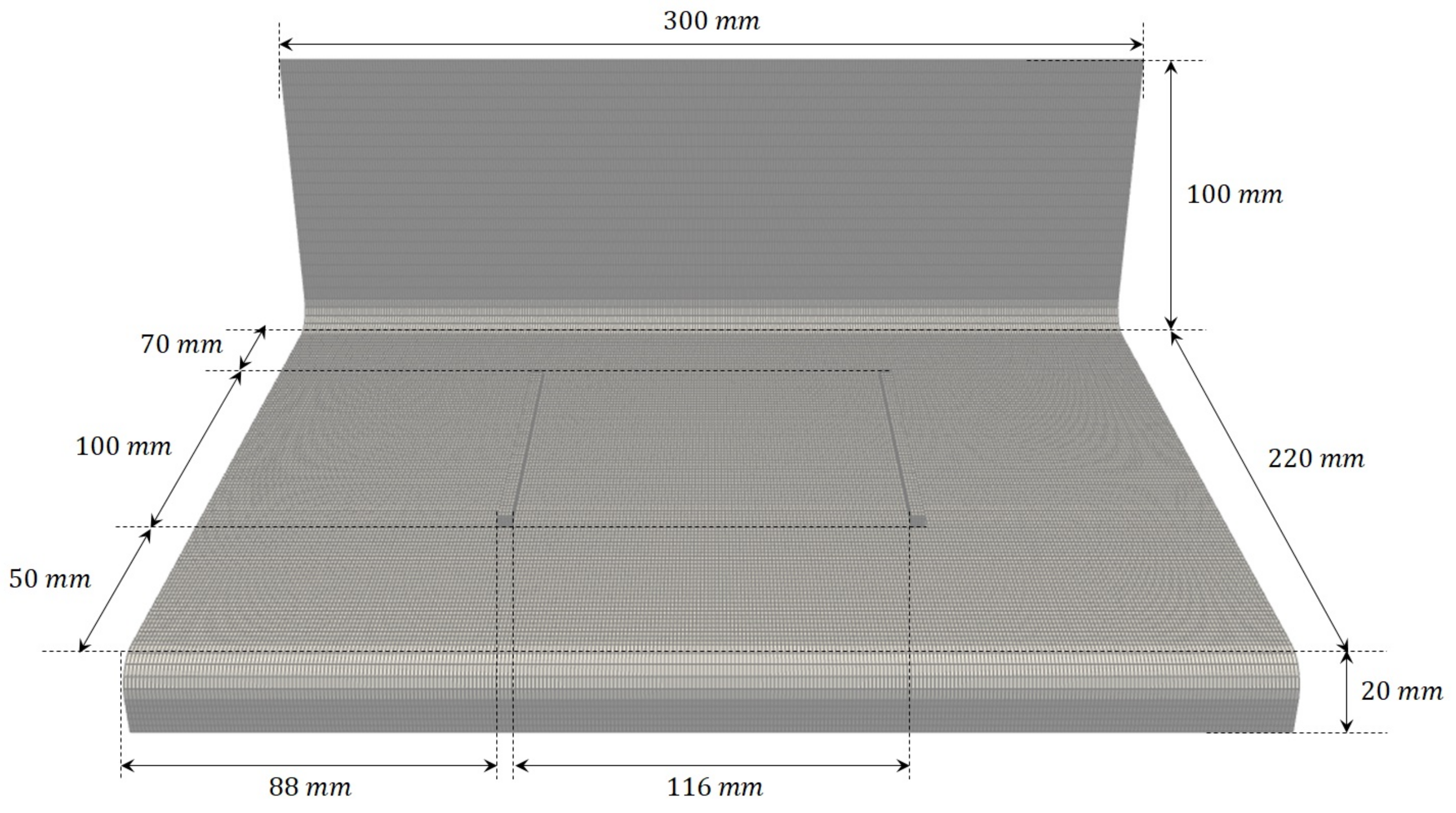
In the case study addressed here, we consider the metallic shell structure whose geometry and dimensions are shown in Figure 3, constituted of steel ($E=210$ GPa, assumed described from an adequate elastoplastic behavior). The structure is being rigidified by printing two stiffeners on it. Each stiffener consists of four printed layers, and, consequently, a sequence of eight unitary operations will define the global process. As it can be noticed, many possibilities exist of sequencing these eight unitary operations, and the final accumulated structure distortion depends on the sequencing choice made. The final state for a particular sequencing choice is shown in Figure 4.

The structure model consists of a quadrilateral elements mesh of $1.76$ mm thickness. The mesh contains about 42,000 nodes. The printed stiffeners are modeled by using solid elements, and are applied at two different locations (left and right stiffeners), four layers in each stiffener (eight unitary operations), using a predefined sequencing. The high-fidelity simulations are carried out by using the commercial software VPS that considers the right material behavior (needing a fine-tuning material calibration) and its integration by using an experienced finite element discretization taking into account the irreversible inelastic (plastic) behavior. For additional details on the considered model and its finite element discretization, the interested reader can refer to the VPS user manual [26].

In this quite simplistic case study, there are many possible sequences. This number grows exponentially when considering more stiffeners, and/or much more layers in each. The simulation of all the possibilities is out of reach in most of industrial applications because each calculation can be computationally expensive (several hours calculation). Each printed layer in each stiffener will modify the structure state (deformation), and the final deformation will strongly depend (due to the nonlinear behavior) on the chosen sequence of unitary operations. Figure 5 shows the states after each of the eight unitary operations when considering the sequence $\{1,2,1,2,1,1,2,2\}$, where 1 refers to a layer applied in the left stiffener and 2 when it is applied on the right stiffener. Because of the software employed, seams are all present in the model, even if they have still not been mechanically activated.

2.3. Proposed Methodology

In this section, we present the methodology which we developed to build a surrogate model of a sequenced process. First, we present how we prepare the data for the model computation. Then, we solve the regression problem with the MLP and with the DMD to finally explain how to use the resulting models.

2.3.1. Data Preparation

The extracted data from the finite elements model are the initial nodes coordinates and their displacements after each operation.

In our case, we want to use the surrogate model to generate all the intermediate structure states for a new sequence $S_k$ (k is the sequence number in the DoE) of size T and initial state $X_k\left(t_0\right)=X_0$. T is the number of unit operations, $T=8$ for all sequences. Thus, for all $i\in \{1,\dots ,T\}$, we need to predict the state $X_k\left(t_i\right)$ taking as input the previous state $X_k\left(t_{i-1}\right)$ when applying the unitary operation $s_k\left(t_{i-1}\right)$.

Thus, the regression reads as:

$$X_k\left(t_i\right)=f\left(X_k\left(t_{i-1}\right),s_k\left(t_{i-1}\right)\right),\forall i\in \{1,\dots ,T\}.$$

(10)

Because the function we search must be the same for all states of the system, we can write Equation (10) by grouping all states of the system in the same matrix, as it is done when applying the DMD

$${\mathbb{X}}_k=f\left({\tilde{\mathbb{X}}}_k,S_k\right),$$

(11)

with ${\tilde{\mathbb{X}}}_k=\left[X_k\left(t_{T-1}\right)\cdots X_0\right]$ and ${\mathbb{X}}_k=\left[X_k\left(t_T\right)\cdots X_k\left(t_1\right)\right]$ respectively the input and the output state matrices (of size $N\times T$) of the system subjected to the sequence $S_k$.

Once again, because the function f must be the same for all tested sequences, i.e., the whole DoE, constituted of $N_C$ simulations, we can concatenate all the input matrices together and all the output matrices together into bigger matrices that we simply note $\tilde{\mathbb{X}}$ and $\mathbb{X}$, both of size $N\times (T\times N_C)$. Thus, the regression problem reads

$$\mathbb{X}=f\left(\tilde{\mathbb{X}},S\right),$$

(12)

where S is the vector concatenating all the sequences, of size $T\times N_C$ and f the generic function. This function is constructed (learned from the data) by using the procedures described in Section 2.3.2.

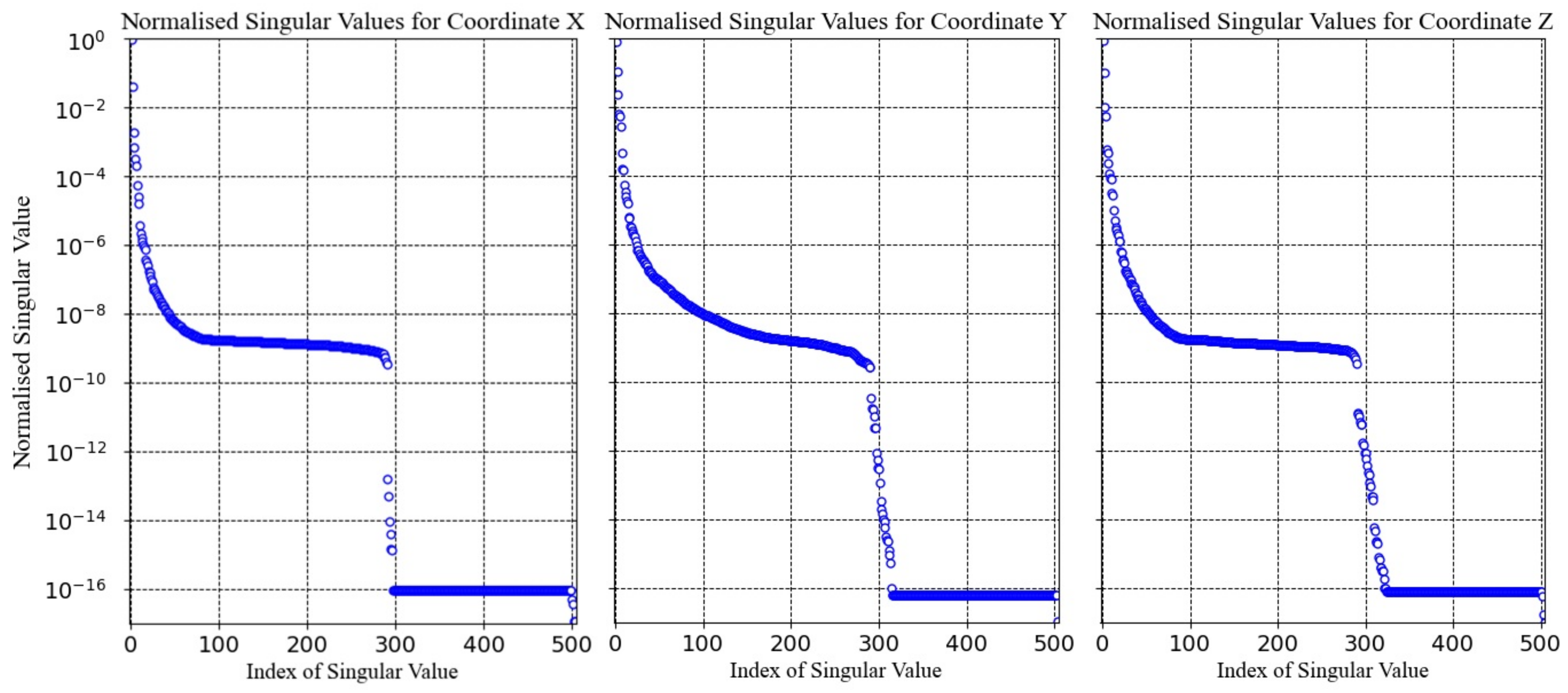
In order to reduce the complexity, we compute the SVD of matrix $\mathbb{X}$, built for each coordinate axis. The normalized singular values related to the three nodal displacements are plotted in Figure 6.

As we can see in these graphs, the singular values decrease very fast, and three modes suffice to reduce the singular values of two orders of magnitude. Thus, we expect approximating reasonably well the structure state (nodal displacements) with a very limited number of vectors of the reduced basis. In addition, $95\%$ of accuracy is attained by employing only the first three modes that will constitute the reduced basis. This reduction is quite impressive: moving from a space of dimension N (the number of nodes) to one involving only three degrees of freedom (the size of the reduced basis) only introduced a $5\%$ loss of accuracy. In what follows, we consider richer bases for obtaining higher accuracy.

Figure 7 plots the approximation error of all the states concerned in the DoE projected into a 5D reduced basis. Even if, as noticed, 5 modes offer excellent performances, errors in the prediction are amplified in posterior operations, and, consequently, it is important to retain a reduced basis that is accurate enough.

Approximation errors when using 5 and 10 modes’ reduced bases are compared in Figure 8. As we can see in this figure, the 5 modes approximation produces a maximum approximation error around $0.025$ mm. To minimize the error growth during the integration (error accumulation), the use of 10 modes seems a better option, and it provides excellent accuracy.

With this choice, each state of the evolving structure can be expressed by a vector with 10 components. In order to address the potential nonlinearities induced by the sequencing and the increase of the structure stiffness, we include in the regression the sequencing as well as the index that identifies the operation within the sequence, as described below:

$${\mathcal{X}}_k={\left(\begin{array}{ccc}{\alpha }_{1,1}& \cdots & {\alpha }_{1,T-1}\\ ⋮& \ddots & ⋮\\ {\alpha }_{10,1}& \cdots & {\alpha }_{10,T-1}\\ s_1& \cdots & s_{T-1}\\ 1& \cdots & T-1\end{array}\right)}_k\mathrm{and}{\mathcal{Y}}_k={\left(\begin{array}{ccc}{\alpha }_{1,2}& \cdots & {\alpha }_{1,T}\\ ⋮& \ddots & ⋮\\ {\alpha }_{10,2}& \cdots & {\alpha }_{10,T}\end{array}\right)}_k$$

(13)

2.3.2. Regression

In order to compute the regression, a valuable route consists of separating the operations performed in the left and the right stiffeners. To improve the predictability capacity even more, one could also cluster the model depending on the existence or not of at least a printed layer in one of the stiffeners as illustrated in Figure 9. It is named the topology clustering in what follows.

• DMD-based regression.

The DMD-based regression reads

$${\mathcal{Y}}^{r/l,c}=A_{r,l}^c{\mathcal{X}}^{r/l,c},$$

(14)

where $\mathcal{Y}$ (resp. $\mathcal{X}$) concatenates the matrices ${\mathcal{Y}}_k$ (resp. ${\mathcal{X}}_k$) related to the right or left stiffeners ($r/l$) and associated with cluster c (in reference to Figure 9).

The problem is solved by using the Tikhonov regularization [27,28] and proceeds by enforcing Equation (14) while adding a penalty related to the norm of the searched matrix A, except for the last two columns afecting the sequencing information contained in the state matrix $\mathcal{X}$. The problem is solved using the Ridge algorithm in the scikit-learn package in Python.

• MLP-based regression.

To set the MLP hyper-parameters, we iterate until obtaining results good enough in the approximation function. This results with:

-

An input and an output layers, respectively constituted of 12 and 10 neurons;

-

2 hidden layers, with 12 neurons per layer;

-

relu the activation function, which is $relu\left(x\right)=max(0,x)$;

-

Adam algorithm [25] to compute weights;

-

the optimization process stops when the score is not improving anymore, according to the scikit-learn documentation [29]

As for the DMD, to solve this problem, we use the class MLPRegressor available in the scikit-learn package in Python.

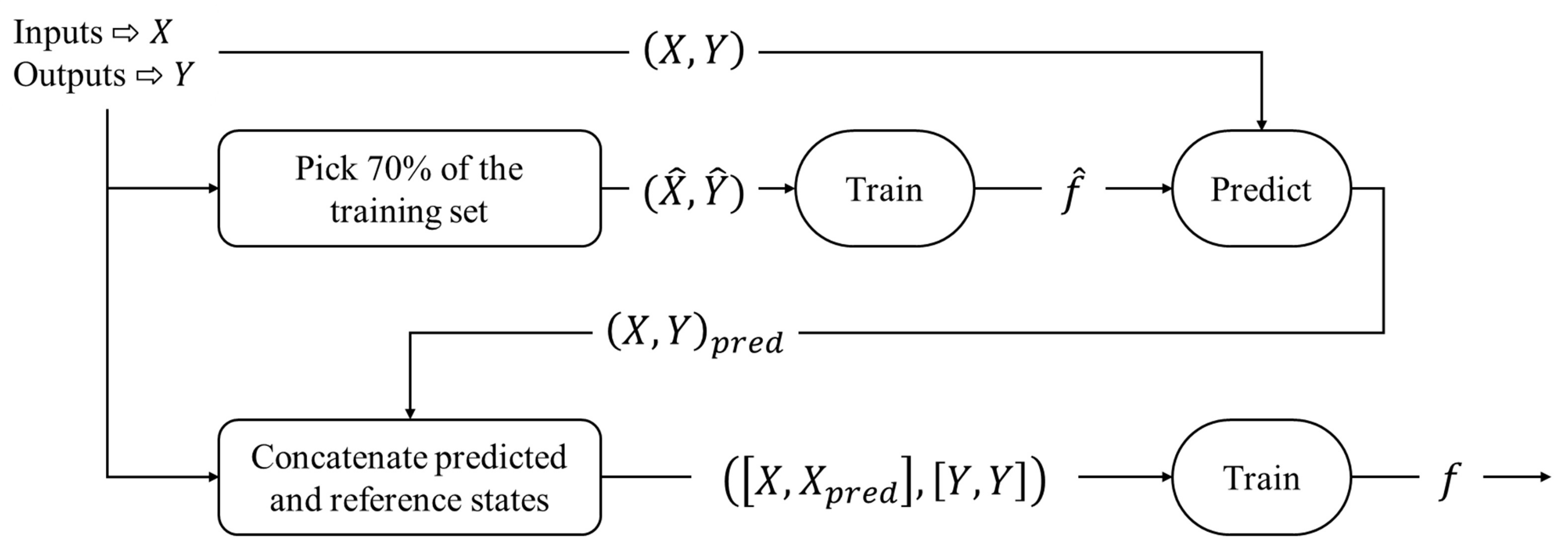
When building this MLP on the whole training dataset, we obtain very unsatisfying results, with an accuracy that degrades when the process advances. To improve it, we build the MLP as a self controlled system: instead of learning with the whole dataset, it learns with $70\%$ of it. Thus, it learns with $70\%$ of $80\%$ of a total of 70 data points, thus 39 data points. Then, we use the resulting MLP to predict the whole training dataset. These predictions are then used as inputs, with the reference inputs, to train a new MLP, whose outputs are the reference states. Thus, the MLP trains with 56 data points and 56 predictions, built with the first MLP trained with only 39 data points. Figure 10 schematizes this training process.

• Dictionary model use.

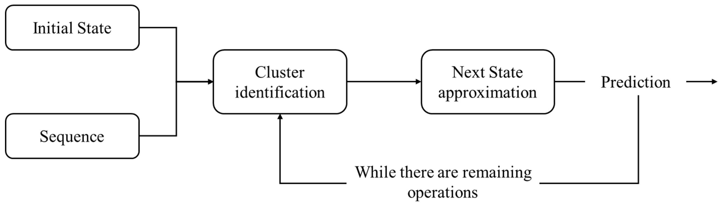
As different models have been learned, when integrating, after each unitary operation, one must identify the model to be employed (right/left and the cluster with respect to Figure 9). The procedure is illustrated in Figure 11.

3. Results

To evaluate the methodology presented in the previous section, we applied all the possible sequences (70 in this case) to the system to constitute the dataset. It has then been divided into two groups: train and test. We performed that selection randomly. In what follows, we only use the training dataset to build the ROMs and the testing dataset to validate them. Whether we applied the regression with the DMD or the MLP, the presented results have been produced with the same methodology, sketched in Figure 12. Section 3.1 presents the results we obtained with the MLP regression and Section 3.2 the results we obtained when using the DMD.

To avoid the impact of very small solutions in the calculation of relative errors, the absolute error in L2-norm is considered. Sometimes, we will give a percentage to discuss the error. It is defined as the maximum error divided by the maximum displacement at each state.

3.1. MLP Results

Figure 13 and Figure 14 show the results we obtained when using the MLP regression, respectively, without and with the topology clustering. These figures plot the maximum error of the approximation obtained by using the ROM and the maximum displacement of the reference solution, at each state. Clustering does not introduce significant advantages when combined with the MLP regression.

Furthermore, as we can see in these graphs, some states are approximated with more than $50\%$ of error. It is too much even for a ROM that aims at keeping and ensuring good accuracy.

Figure 15 shows a 3D view of one of the worst approximations we obtained with the MLP regression. As it can be seen in this picture, maximum errors are essentially concentrated at the corners of the metal sheet for the first five states. The prediction quality should be improved to fulfill standard tolerances.

For that purpose, we searched for better neural network hyper-parameters. Results are reported in

Table 1. Results for different choices of hyper-parameters for the neural network.

Number of Hidden Layers	Number of Neurons	Activation Function	Maximum Error
2	$(12,12)$	relu	2.5 mm
2	$(20,20)$	relu	5.5 mm
2	$(40,40)$	relu	3 mm
2	$(20,12)$	relu	3 mm
2	$(40,20)$	relu	2.5 mm
2	$(40,20)$	logistic	4.5 mm
2	$(40,20)$	tanh	6.5 mm
2	$(40,20)$	identity	2.9 mm
3	$(12,12,12)$	relu	4 mm
3	$(40,40,40)$	relu	4 mm
4	$(12,12,12,12)$	relu	2.8 mm
4	$(40,40,40,40)$	relu	2.8 mm

. According to this table, the choice for the neural network hyper-parameters, for this type of architecture and data, seems quite optimal.

3.2. DMD Results

Figure 16 and Figure 17 show the results we obtained using the DMD respectively without and with topology-based clustering. They plot the maximum error of the approximation provided by the ROM and the maximum displacement of the reference solution at each state. This maximum absolute error remains smaller than the one obtained with the MLP regression.

Furthermore, as we can see comparing these two figures, the topology clustering leads to a better approximation, justifying its consideration when using the DMD-based regression.

In Figure 17, the maximum error does not exceed $10\%$ of the maximum displacement. Furthermore, the absolute error is always less than 0.7 mm. For a metal sheet of around 300 mm in size, this error could be acceptable in certain applications.

In addition to this quite reduced absolute error, we can see that the maximum error during the whole sequence seems to stay globally stable, without exhibiting net accumulation.

Figure 18 shows a 3D view of the worst approximation we obtained with the DMD model. As we can see in this picture, maximum errors are again essentially concentrated at the corners of the metal sheet.

4. Conclusions

The presented paper addressed the recurrent issue of creating reduced order models of processes involving sequencing. Evaluating the effect of all the possible processing sequences represents an unattainable objective because of the associated curse of dimensionality.

Thus, in general, processing designs are based on simplified models, the use of existing heuristics and knowledge, or the exploration of small regions of the design space, all of them underperforming.

On the other hand, the possibility of having a real-time accurate predictor of the effect of any sequence on the final properties and performances could represent an impressive opportunity in engineering.

In the present paper, we succeeded to accomplish that challenge by combining different ideas and methodologies, whose performances were proven in a case study of industrial relevance, in particular:

• Global solutions can be represented in a reduced basis, that is, the dimensionality of the thermomechanical fields remains much smaller than the number of processing sequences. We proved that a quite reduced number of modes allows for representing the states of the distorted structure.
• More than trying to link the sequencing with the final state of the structure, facing the sequencing parametrization issue, here we proposed the construction of a parametric transfer function related to a unitary operation. From a given state, it can predict the next state after the unitary operation.
• We proposed employing different regressions for accomplishing that modeling, in particular the DMD and the MLP, both working quite well, with the performances of the former improved by using clustering, and the ones of the last improved by using a self-controlling procedure.
• The models were successfully learned and they performed very well in the data reserved for validation purposes.

Future works will address more complex scenarios, propose an improved clustering, better address nonlinear behaviors, and improve the DoEs, as well as the approximation of other processes involving sequencing, as for example spot-welding.

References

- Deng, D.; Murakawa, H. FEM prediction of buckling distortion induced by welding in thin plate panel structures. Comput. Mater. Sci. 2008, 43, 591–607. [Google Scholar] [CrossRef]
- Gannon, L.; Liu, Y.; Pegg, N.; Smith, M. Effect of welding sequence on residual stress and distortion in flat-bar stiffened plates. Mar. Struct. 2010, 23, 385–404. [Google Scholar] [CrossRef]
- Wärmefjord, K.; Söderberg, R.; Lindkvist, L. Strategies for optimization of spot welding sequence with respect to geometrical variation in sheet metal assemblies. In Proceedings of the ASME 2010 International Mechanical Engineering Congress and Exposition, Vancouver, BC, Canada, 12–18 November 2010; pp. 569–577. [Google Scholar]
- Mehnen, J.; Ding, J.; Lockett, H.; Kazanas, P. Design study for wire and arc additive manufacture. Int. J. Prod. Dev. 2014, 19, 2–20. [Google Scholar] [CrossRef]
- Josten, A.; Höfemann, M. Arc-welding based additive manufacturing for body reinforcement in automotive engineering. Weld. World 2020, 64, 1449–1458. [Google Scholar] [CrossRef]
- Chinesta, F.; Leygue, A.; Bordeu, F.; Aguado, J.V.; Cueto, E.; Gonzalez, D.; Alfaro, I.; Ammar, A.; Huerta, A. PGD-based computational vademecum for efficient design, optimization and control. Arch. Comput. Methods Eng. 2013, 20, 31–59. [Google Scholar] [CrossRef]
- Chinesta, F.; Keunings, R.; Leygue, A. The Proper Generalized Decomposition for Advanced Numerical Simulations: A Primer; Springer briefs in Applied Sciences and Technology; Springer: Berlin/Heidelberg, Germany, 2014. [Google Scholar]
- Chinesta, F.; Huerta, A.; Rozza, G.; Willcox, K. Model Order Reduction. In Encyclopedia of Computational Mechanics, 2nd ed.; Stein, E., de Borst, R., Hughes, T., Eds.; John Wiley & Sons Ltd.: Hoboken, NJ, USA, 2015. [Google Scholar]
- Hesthaven, J.S.; Ubbiali, S. Non-intrusive reduced order modeling of nonlinear problems using neural networks. J. Comput. Phys. 2018, 363, 55–78. [Google Scholar] [CrossRef] [Green Version]
- Pulch, R.; Youssef, M. Machine learning for trajectories of parametric nonlinear dynamical systems. J. Mach. Learn. Model. Comput. 2020, 1. [Google Scholar] [CrossRef]
- Anderson, J.A. Simple Neural Network Generating an Interactive Memory. Math. Biosci. 1972, 14, 197–220. [Google Scholar] [CrossRef]
- Schmid, P.J. Dynamic mode decomposition of numerical and experimental data. J. Fluid Mech. 2010, 656, 5–28. [Google Scholar] [CrossRef] [Green Version]
- Golub, G.H.; Reinsch, C. Singular value decomposition and least squares solutions. Linear Algebra 1971, 656, 134–151. [Google Scholar]
- Henry, E.R.; Hofrichter, J. Singular value decomposition: Application to analysis of experimental data. Methods Enzymol. 1992, 210, 129–192. [Google Scholar]
- Wall, M.E.; Rechtsteiner, A.; Rocha, L.M. Singular value decomposition and principal component analysis. In A Practical Approach to Microarray Data Analysis; Springer: Berlin/Heidelberg, Germany, 2003; pp. 91–109. [Google Scholar]
- Martin, C.D.; Porter, M.A. The extraordinary SVD. Linear Algebra 2012, 119, 838–851. [Google Scholar]
- Schmid, P.J.; Li, L.; Juniper, M.P.; Pust, O. Applications of the dynamic mode decomposition. J. Comput. Dyn. 2011, 25, 249–259. [Google Scholar] [CrossRef]
- Tu, J.H.; Rowley, C.W.; Luchtenburg, D.M.; Brunton, S.L.; Kutz, J.N. On dynamic mode decomposition: Theory and applications. J. Comput. Dyn. 2014, 1, 391–421. [Google Scholar] [CrossRef] [Green Version]
- Williams, M.O.; Kevrekidis, I.G.; Rowley, C.W. A data-driven approximation of the koopman operator: Extending dynamic mode decomposition. J. Nonlinear Sci. 2015, 25, 1307–1346. [Google Scholar] [CrossRef] [Green Version]
- Proctor, J.L.; Brunton, S.L.; Kutz, J.N. Dynamic mode decomposition with control. SIAM J. Appl. Dyn. Syst. 2016, 15, 142–161. [Google Scholar] [CrossRef] [Green Version]
- Qin, T.; Wu, K.; Xiu, D. Data driven governing equations approximation using deep neural networks. J. Comput. Phys. 2019, 395, 620–635. [Google Scholar] [CrossRef] [Green Version]
- Medsker, L.R.; Jain, L.C. Recurrent neural network. Des. Appl. 2001, 5. [Google Scholar]
- Schmidhuber, J. Deep learning in neural networks: An overview. Neural Netw. 2015, 61, 85–117. [Google Scholar] [CrossRef] [PubMed] [Green Version]
- Bengio, Y.; Goodfellow, I.; Courville, A. Deep Learning; MIT Press: Cambridge, MA, USA, 2017. [Google Scholar]
- Kingma, D.P.; Ba, J. Adam: A method for stochastic optimization. arXiv 2014, arXiv:1412.6980. [Google Scholar]
- Virtual Performance Solution 2018—Reference Manual. Available online: https://myesi.esi-group.com/downloads/software-documentation/virtual-performance-solution-2018-reference-manual-online (accessed on 28 May 2021).
- Calvetti, D.; Reichel, L. Dynamic mode decomposition with control. BIT Numer. Math. 2003, 43, 263–283. [Google Scholar] [CrossRef]
- Rifkin, R.M.; Lippert, R.A. Notes on Regularized Least Squares. 2007. Available online: https://dspace.mit.edu/handle/1721.1/37318 (accessed on 28 May 2021).
- Scikit-Learn MLPRegressor—Reference Manual. Available online: https://scikit-learn.org/stable/modules/generated/sklearn.neural_network.MLPRegressor.html?highlight=mlpregressor#sklearn.neural_network.MLPRegressor (accessed on 28 May 2021).
Figure 1.
The red screw cannot join the two parts because of the screwing order.
Figure 2.
Example of a multi-layer perceptron.
Figure 3.
Metallic structure considered in the present case study.
Figure 4.
Final state related to an 8-unitary operations sequence (displacements ).
Figure 5.
High-fidelity simulation of the sequence (displacements for visualization). Both stiffeners are placed from the beginning on the sheet, and each layer of them is sequentially mechanically activated.
Figure 6.
Normalized singular values related to the three nodal displacements.
Figure 7.
Graph: Maximum modal approximation error with respect to the maximum displacement when using five modes. Picture: Reduced approximation of the deformed structure (displacements ).
Figure 8.
Approximation error when using 5 and 10 modes in the reduced basis.
Figure 9.
Cases with at least one layer was printed (red) or no layer printed (white).
Figure 10.
Learning process for the self controlled MLP.
Figure 11.
Prediction process for the dictionary model.
Figure 12.
ROM generation workflow.
Figure 13.
Maximum prediction error and maximum displacement for the MLP regression without topology clustering.
Figure 14.
Maximum prediction error and maximum displacement for the MLP regression with topology clustering.
Figure 15.
MLP approximation of sequence compared with the reference solution (displacements for visualization).
Figure 16.
Maximum prediction error and maximum displacement for the DMD approximation without topology clustering.
Figure 17.
Maximum prediction error and maximum displacement for the DMD approximation with topology clustering.
Figure 18.
DMD approximation of sequence with its reference (displacements for visualization).