Education-to-Skill Mapping Using Hierarchical Classification and Transformer Neural Network

Abstract

Skills gained from vocational or higher education form an essential component of country’s economy, determining the structure of the national labor force. Therefore, knowledge on how people’s education converts to jobs enables data-driven choices concerning human resources within an ever-changing job market. Moreover, the relationship between education and occupation is also relevant in times of global crises, such as the COVID-19 pandemic. Healthcare system overload and skill shortage on one hand, and job losses related to lock-downs on the other, have exposed a necessity to identify target groups with relevant education backgrounds in order to facilitate their occupational transitions. However, the relationship between education and employment is complex and difficult to model. This study aims to propose the methodology that would allow us to model education-to-skill mapping. Multiple challenges arising from administrative datasets, namely imbalanced data, complex labeling, hierarchical structure and textual data, were addressed using six neural network-based algorithms of incremental complexity. The final proposed mathematical model incorporates the textual data from descriptions of education programs that are transformed into embeddings, utilizing transformer neural networks. The output of the final model is constructed as the hierarchical classification task. The effectiveness of the proposed model is demonstrated using experiments on national level data, which covers whole population of Lithuania. Finally, we provide the recommendations for the usage of proposed model. This model can be used for practical applications and scenario forecasting. Some possible applications for such model usage are demonstrated and described in this article. The code for this research has been made available on GitHub.

1. Introduction

The analysis of country-wide employment and education data is of great practical importance. An accurate evaluation of relationships between education and employment allows for a better forecast of human skill supply. Prediction of quantity and structure of human skill allows for a better planning and preparation as well as change negative tendencies of socio-economic phenomenon [1]. Moreover, economic changes transform employment and occupations; therefore, a significant part of people face a necessity to upskill and redeploy [2]. In these circumstances, knowledge on how education is related to employment and how obtained education transforms into jobs is very important. It comes as no surprise why national (e.g., UK organization NESTA [3]) and international organizations (e.g., EU agency of The European Centre for the Development of Vocational Training [4]) are investing in perfecting human skill forecasting.

At first sight, education-to-skill mapping seems to be a simple task; it might be possible to approximate the most likely occupation by estimating frequencies of graduates’ employment. However, looking closely, this task is rather complex.

The first challenge is the complexity of administrative data. Education programs are short-lived and constantly changing as the number of new programs tends to grow, and some old programs are terminated or rewritten. With a simplified approach, it is impossible to map new education programs to occupations as there is no digitized historical data in machine-readable format. Furthermore, in some instances, there are too few actual graduates throughout certain programs’ lifetimes. Applying econometric modeling or simple machine learning classification algorithms to education program data is challenging as the huge number of programs, being categorical in their nature, transforms to highly sparse and unbalanced input data and this affects the accuracy of the predictions. Another challenge related to education data is the fact that residents are diverse and might complete several education programs, that in combination make up a unique set of qualifications and skills.

Data about residents’ employment is not simple either. For instance, residents might have more than one job at a time, have several different jobs during their career, and residents are likely to have more skills and higher-level jobs as their career progresses. Additional challenges arise from rare occupations, which create imbalances in the data. For example, such professions as divers, radio and TV show hosts, and meteorologists, are normally occupied by a very small number of residents on the national scale. Thus, a simplified estimation of the relationship between education and occupation would generalize poorly because of the complexity of the problem.

Finally, globally devastating events, such as the COVID-19 pandemic [5], financial crises [6], and climate change [7] have overwhelming effects on human resources around the world. However, the econometric time-series forecasting models in this context perform rather poorly: being based on historical data, they can not reliably account for the unexpected events [8,9]. Thus, in these circumstances, it is important to have a complete set of various scenario generation tools, including machine learning methods [6].

The aim of this research is to propose a mathematical model that would not only map education to occupations accurately enough, but also have other practical applications. To achieve this aim, the mathematical model is proposed based on state-of-the-art models in the field. Empirical experiments based on national level data were performed, and the analysis of results was also accomplished in order to progress with well-established scientific concepts. Lastly, practical application experiments with resulting models were performed to provide additional insights into possible applications.

The rest of the paper is organized as follows: in Materials and Methods, Section 2, the mathematical methods are described as well as proposed models, experimentation data, architecture of models, text pre-processing and computational infrastructure. Results and Discussion, Section 3, presents and discusses the results of experiments and examples of applications. Finally, Conclusions, Section 4, closes the article.

2. Materials and Methods

2.1. Mathematical Models

This section provides with information on main notations for the proposed model.

2.1.1. Deep Neural Networks

Education-to-skills mapping is considered as a supervised learning classification problem. The task of supervised learning in the machine learning context is to learn a mapping $f_{\theta }:X\subset {\mathbb{R}}^{d_x}\to Y\subset {\mathbb{R}}^{d_y}$ from the given dataset $\mathcal{D}=\left\{(x^{\left(i\right)},y^{\left(i\right)})\right|1\le i\le N\}$. X denote the input space and Y denote the label space. Here, $x^{\left(i\right)}\in X$ is an ith input sample and $y^{\left(i\right)}\in Y$ is the ith corresponding label sample [10].

2.1.2. Deep Neural Network

In this research, a fully connected neural network (DNN) is considered [11]. The network performs an operator function $f_{\theta }:X\subset {\mathbb{R}}^{d_x}\to Y\subset {\mathbb{R}}^{d_y}$. The composition of M non-linear transformations (layers) are considered, where $M-1$ will be hidden layers and the last one will be an output layer. The vector is fed to the model and can be defined as $X^0=X$.

The m-th layer has $n_m$ of unknown parameters $\theta \subset {\mathbb{R}}^{n_{m-1}+1}$, receives an input vector $X^{m-1}\in {\mathbb{R}}^{n_{m-1}}$ and transforms it into the vector $X^m\in {\mathbb{R}}^{n_m}$ by applying the linear transformation, followed by a component-wise (non-linear) activation function $\sigma$:

$$X^m=\sigma \left({\theta }^m{X}^{m-1}\right),$$

(1)

where ${\theta }^m\in {\mathbb{R}}^{n_m\times n_{m-1}+1},1\le m\le M$, $X^m$—input for the $(n+1)$-th layer, and the ReLU activation function: $\sigma \left(x\right)=relu\left(x\right)=max(0,x)$ [11].

The output function $\mathcal{S}$ depends on the classification task; in a case of single label classification it would be the softmax function, but in our case of multi-label classification would be the sigmoid function:

$$\mathcal{S}\left(y\right)=\left(\sigma \left(y_1\right),\dots ,\sigma \left(y_{d_y}\right)\right).$$

(2)

where $\sigma \left(x\right)=sigmoid\left(x\right)=exp\left(x\right)/(1+exp(x\left)\right)$.

2.1.3. Parameters estimation

The quality of the proposed model $f_{\theta }$ is measured with loss function ${\mathcal{L}}_{\theta }(y,f\left(x\right|\theta ))$. In the study, $f_{\theta }$ is the deep neural network with unknown parameters of $\theta \in \mathsf{\Theta }\subset {\mathbb{R}}^{d_{\theta }}$. Since the model $f_{\theta }$ is parametric, the unknown parameters are updated using the gradient of loss function: ${\nabla }_{\theta }{L}_{\theta }$ [11]. In simple form, parameters $\theta$ are updated iteratively:

$${\theta }_{t+1}={\theta }_t-\eta ·{\nabla }_{\theta }{\mathcal{L}}_{\theta t}$$

(3)

where $\eta$ is learning rate or the size of the steps to reach minimum loss, t-iteration number [11].

For the process to converge successfully, a proper learning rate has to be applied for avoiding being trapped in local minima [11]. Usually, there are multiple optimization techniques that can be employed to solve this problem. In this study, Adaptive Moment Estimation (from here after abbr. as Adam) optimization was used. Adam computes learning rates for each parameter, using information on exponentially decaying averages of past gradients [11].

Let gradient of loss function to the ith parameter ${\theta }_i$ at iteration t be: $g_{t,i}={\nabla }_{\theta }{\mathcal{L}}_{\theta t,i}$. Then

$$\begin{array}{c}\hfill \begin{array}{cc}\hfill m_t& ={\beta }_1{m}_{t-1}+(1-{\beta }_1)g_t\hfill \\ \hfill v_t& ={\beta }_2{v}_{t-1}+(1-{\beta }_2)g_t^2\hfill \end{array}\end{array}$$

(4)

where $m_t$ and $v_t$ are estimates of the first moment (the mean) and the second moment (the uncentered variance) of the gradients $g_t$. ${\beta }_1$ and ${\beta }_2$ are hyper-parameters and usually values of 0.9 and 0.999, respectively, are used [11].

As $m_t$ and $v_t$ are initialized as 0’s vectors, they are biased towards zero, especially during the initial state. These biases are corrected by computing first and second moment estimates such that [11]:

$$\begin{array}{c}\hfill {\widehat{m}}_t={\displaystyle \frac{m_t}{1-{\beta }_1^t}},{\widehat{v}}_t={\displaystyle \frac{v_t}{1-{\beta }_2^t}}\end{array}$$

(5)

The Adam update rule $t\ge 1$:

$$\begin{array}{c}\hfill {\theta }_{t+1}={\theta }_t-{\displaystyle \frac{\eta }{\sqrt{{\widehat{v}}_t}+ϵ}}{\widehat{m}}_t\end{array}$$

(6)

Here, $ϵ$ is smoothing term (avoiding zero in denominator) usually set to ${10}^{-8}$.

2.1.4. Model Performance Evaluation

To evaluate model performance metrics such as Accuracy (abbr. Acc), Precision (abbr. Pr), Recall (abbr. Re) and F1 are adopted. For the estimations of metrics TP (true positive, the label was 1, 1 was predicted), TN (true negative, label was 0, 0 was predicted), FP (false positive, label was 0, 1 was predicted), FN (false negative, label was 1, 0 was predicted) are used [10].

Accuracy metric is defined as:

$$\mathrm{Acc}=\frac{\mathrm{TP}+\mathrm{TN}}{\mathrm{TP}+\mathrm{TN}+\mathrm{FP}+\mathrm{FN}}$$

(7)

In some instances, accuracy metric is sufficient, but often it may be misleading, especially in classification task with many classes or dealing with imbalanced data. When classes are sparse and imbalanced resulting accuracy value is dominated by majority group, such as 0 labels [12]. Therefore, additional metrics should be adopted.

Precision measures the percentage of the positively predicted samples, that are actually labeled as 1. Precision considers the number of negative samples and can answer the question of how many real predictions were in the prediction sample. Recall is a measure for the positive group that was correctly predicted to be 1 and can answer the question of how many of positive labels model detected [12].

$$\mathrm{Pr}=\frac{\mathrm{TP}}{\mathrm{TP}+\mathrm{FP}},\mathrm{Re}=\frac{\mathrm{TP}}{\mathrm{TP}+\mathrm{FN}}$$

(8)

F1 score is the harmonic mean of the precision and recall, defined as:

$$\mathrm{F}1=2\frac{\mathrm{Pr}·\mathrm{Re}}{\mathrm{Pr}+\mathrm{Re}}$$

(9)

2.1.5. Multi-Label Learning

Multi-class classifiers can handle many numbers of classes, but only exactly one class can appear in each sample. A multi-label classifier is an extension of multiclass classifiers that can have multiple classes in each sample (number of classes in each sample is between zero and total number of different classes). Thus, multi-label classification can be defined as machine learning task that classifies data into many classes where each class can co-occur simultaneously. In other words, a multi-label task is the problem where each example is associated with a set of labels [10].

Suppose $X\in {\mathbb{R}}^{d_x}$ denotes $d_x$-dimensional instance space, and $Y=(y_1,y_2,\dots ,y_{d_y})\in {\mathbb{R}}^{d_y}$ denotes the label space with $d_y$ possible class labels. The task of multi-label learning is to learn an operator $h:X\to {(0,1)}^{d_y}$ from the training set $D_{tr}=\left\{(X^{\left(i\right)},Y^{\left(i\right)})\right|1\le i\le N\}$. For each multi-label pair example: $X^{\left(i\right)}$ is a $d_x$-dimensional feature vector $X^{\left(i\right)}=(x_1^{\left(i\right)},x_2^{\left(i\right)},\dots ,x_{d_x}^{\left(i\right)})$ and $Y^{\left(i\right)}$ is the set of labels associated with $X^{\left(i\right)}$. For any unseen instance $X^{\left(i\right)}\in X$, the multi-label classifier $h(·)$ predicts $h\left(X^{\left(i\right)}\right)\subseteq Y$ as the set of proper labels for $X^{\left(i\right)}$. The key idea of multi-label learning is decomposition of the problem into number of independent binary classification problems, where each classifier corresponds to a possible label [10].

The classification to set $\{1,..,d_y\}$ is performed after application of threshold. The threshold of predicted value by the model is noted as [10]:

$$\begin{array}{c}\hfill c_j^{\left(i\right)}=\left\{\begin{array}{cc}0,\hfill & \mathrm{if}{\widehat{y}}_j^{\left(i\right)}<T_j\hfill \\ 1,\hfill & \mathrm{if}{\widehat{y}}_j^{\left(i\right)}\ge T_j\hfill \end{array}\right.,c_j^{\left(i\right)}\in \{0,1\},\end{array}$$

(10)

where $j=1,\dots ,d_y,i=1,\dots ,N$, and $T_j$ acts as a threshold which dichotomizes the label space into relevant and irrelevant label sets.

In multi-label classification tasks, each class performance should be evaluated independently from the other. Common practice is to use sigmoid activation for the last layer that transforms the input into a probability range $(0,1)$ for every class (separate probabilities).

The loss function for the multi-label problem (Cross-entropy loss ($\mathcal{L}$)):

$$\begin{array}{c}\hfill {\mathcal{L}}_{CE}(y^{\left(i\right)},{\widehat{y}}^{\left(i\right)})=-\sum _{c=1}^{d_y}{y}_c^{\left(i\right)}log\left({\widehat{y}}_c^{\left(i\right)}\right)\end{array}$$

(11)

where $y_c^{\left(i\right)}\in \{0,1\}$ is a binary class label, ${\widehat{y}}_c^{\left(i\right)}\in (0,1)$ is an estimate of the probability of the positive class [11].

2.1.6. Class Imbalance Problem

Although class imbalance results from lack of available data, imbalanced data also appears in the cases of classification tasks for many classes or sparse class data, where majority labels, having a nature of one-hot encoding, is 0. High class imbalance is natural in many real-world datasets for classification tasks, such as image recognition, medical diagnosis, and fraud detection (summarised by, e.g., [13]).

The general measure of class imbalance in research is defined:

$$\begin{array}{c}\hfill \begin{array}{c}\hfill \rho =\frac{ma{x}_c\left\{\right|S_c\left|\right\}}{mi{n}_c\left\{\right|S_c\left|\right\}}\end{array}\end{array}$$

(12)

where $\rho$ is maximum imbalance between class, $S_c$ is a set of examples in class c, and $ma{x}_c\left\{\right|S_c\left|\right\}$ and $mi{n}_c\left\{\right|S_c\left|\right\}$ is maximum and minimum class size over all classes. For example, if maximum class size is 1000 and minimum class size is 10, then $\rho$ is 100.

Even though class imbalance is widespread, the general majority of classifiers operate on an assumption that classes in the training dataset are balanced. Therefore, in cases of class imbalance, many classifiers exhibit bias towards the classes that represent majority cases due to its increased prior probability. In this case, the classifier might ignore minority classes that tend to be misclassified [12].

Anand and colleagues showed that class imbalance interferes with backpropagation, resulting in much smaller length of gradient component in minority classes [14]. Thus, majority class dominates net gradient, which is responsible for weights adjustment. This results in reduced loss only for large class groups [14].

In this study, we tackle the data imbalance issue using specific methods, namely: focal loss, structuring output as hierarchy and transforming input data as text embeddings.

2.1.7. Focal Loss

With a large number of classes, true negatives can easily overwhelm training and the loss might become unrealistically small for false negatives. Likewise, if the dimension number of the output is large (there are many classes of labels) and each training sample has only few cases of some classes, the loss would encourage ignoring these few cases. Nonetheless, those cases might be extremely important for the model’s predictive performance.

One way to solve this is by using focal loss. Focal loss was originally proposed as an effective loss function for the image processing–object detection problem. The problem with object detection might occur in cases when rare objects are missed because the background occupies a large part of the image. Thus, detection fails because extreme foreground/background class imbalance prevents learning. Yet research shows that focal loss is useful not only for visual analysis but also in general multiclass classification tasks of imbalanced class conditions [15].

Focal loss improves the classifier by configuring the loss function with modulating factor. Focal loss can be defined as:

$$\begin{array}{c}\hfill {\mathcal{L}}_F(y^{\left(i\right)},{\widehat{y}}^{\left(i\right)})=-\sum _{c=1}^{d_y}{\alpha }_c{(1-{\widehat{y}}^{\left(i\right)})}^{\gamma }{y}_c^{\left(i\right)}log\left({\widehat{y}}_c^{\left(i\right)}\right)\end{array}$$

(13)

where $y_c^{\left(i\right)}\in \{0,1\}$ is a binary class label, ${\widehat{y}}_c^{\left(i\right)}\in (0,1)$ is an estimate of the probability of the positive class, $\gamma$ is the focusing parameter, $\alpha$ is a hyperparameter that weights the positive class up or down $\alpha \in [0,1]$ [11,15,16].

The hyperparameter $\gamma$ prevents overwhelming loss with frequent cases focusing the model on instances with fewer classes. The higher the $\gamma$, the higher the rate at which easy-to-classify examples are down-weighted. The weighted binary cross-entropy loss is special case of focal loss when $\gamma =0$. Criteria to choose $\gamma$ value is the degree of data imbalance [15,16].

2.1.8. Hierarchical Classification

Vast majority of machine learning applications for classification task disregards hierarchical information. Although many classification problems, especially problems involving many classes, might inherit natural hierarchical structure of classes [17]. It might be useful to employ the hierarchical data structure to improve prediction as larger classes on the top level of hierarchy are more easily predicted. The hierarchy is also useful in deployment of the model: it can be adapted for different circumstances, where there is a need to predict a shallow level of hierarchy [17,18].

Silla and Freitas (in 2011 [18]) have grouped hierarchical classification into three main categories: flat, local and global. The flat classifier ignores the hierarchy and classifies only leaf nodes assuming that ancestor classes are also implicitly assigned. The local classifier system employs set of local classifiers (classifier per level, one binary classifier per node or classifier per parent node). The global classifier uses a single classifier to deal with the entire class hierarchy.

The choice of the classifier depends on specific problems. Generally, local classifiers provide more options to modulate the relationship between parent and leaf. The weakness of such an approach is the complexity of the model, as classifiers tend to grow with the additional hierarchy layers. Moreover, local classifiers might suffer from inconsistency in class predictions across different levels, which needs to be approached with additional correction methods (e.g., hierarchy pruning, thresholds, etc.) [18]. Global classifiers do not entail such challenges as the hierarchy structure is learned during the learning process [18].

2.1.9. Text Embedding

Text embedding might be defined as a vector representation of words that contains information about both semantic and syntactic meaning [19]. Text embeddings allow us to efficiently represent textual data in vector space. Unlike one-hot vectors, the embedded text is not sparse. Moreover, it contains information about relatedness between categories. Embeddings not only represent words, phrases or sentences in numeric form but also preserve additional information: the meaning of words and its relatedness to each other [19].

More formally, let W be size of dictionary, F be new size of selected feature dimension, then the one-hot word representation x is mapped to new vector $e_{1\times F}^{\left(i\right)}=x_{1\times W}^{\left(i\right)}{E}_{W\times F}$. The matrix $E_{W\times F}$ is called embeddings matrix, and $e_{1\times F}^{\left(i\right)}$ is word $x_{1\times W}^{\left(i\right)}$ embedding.

The relatedness between words $x^{\left(i\right)}$ and $x^{\left(j\right)}$ can also be interpreted in several ways. The taxonomy relatedness appears between words because they share many common features (for example, words “teach” and “educate” are related because both are members of the same category). The thematic relatedness emerges when even dissimilar words frequently co-appear in the same context (for example, words “student” and “diploma” do not belong to the same category, yet they are closely related to each other). The thematic relatedness includes some of the features of taxonomy relatedness. The thematic relatedness assumes context overlap as indication of feature overlap [20].

The larger the corpus available for the embedding training, the better embedding is performing in the NLP task. Embedding can be used as integrated layer in the deep learning model or as transfer learning. Transfer learning in this case consists of using embedding model pre-trained on a large text corpus. The practical reason for it is that a very large corpus is not available for a specific NLP task. Using pre-trained embedding, one needs only to fine tune to adapt it to the specific task [21].

2.1.10. Transformer Neural Networks

Text embedding can be performed using various techniques. One example of such a technique is the use of transformer architecture. Transformers might be used in many practical settings, such as language modelling, speech recognition, image and music analysis [22].

Transformer is created by modifying parts of an auto-encoder [23]. The auto-encoder maps input to the output, and dimensions of input and output might be different. It consists of two important blocks: encoder and decoder [24]. The transformer uses the same logic of auto-encoder just replacing fully-connected or convolutional layers with attention function that gives specific weights over the input sequence. The advantage of attention function is that it allows the encoder to proceed to longer sequences, which is very important to NLP tasks.

More formally, the attention transformation $A(Q,K,V):{\mathbb{R}}^{d_x}\to {\mathbb{R}}^{d_v}$ is used in the transformer neural network. First, the input is decomposed by calculating the three matrices $Q={\theta }^{Q}x$, $K={\theta }^{K}x$, and $V={\theta }^{V}x$, then the attention is calculated:

$$A(Q,K,V)=softmax\left(cQ{K}^T\right)V$$

(14)

where $c=1/\sqrt{d_k}$ the normalization constant, $d_k$ is the dimension of K. The Q matrix is called the query, K—the keys, and V—the values matrices.

Equivalent to a fully connected neural network, the attentions can be combined, which is known as multi-head attention $MHA(Q,K,V)$, which enables us to jointly combine the information from different representations of input at different positions.

$$\begin{array}{ccc}\hfill MHA(Q,K,V)& =& (A_1,...,A_h){\theta }^Y\hfill \end{array}$$

(15)

$$\begin{array}{ccc}\hfill \mathrm{where}{A}_i& =& A(Q{\theta }_i^Q,K{\theta }_i^K,V{\theta }_i^V)\hfill \end{array}$$

(16)

Here, the projections are parameter matrices ${\theta }_i^Q\in {\mathbb{R}}^{d_x\times d_q}$, ${\theta }_i^K\in {\mathbb{R}}^{d_x\times d_k}$, ${\theta }_i^V\in {\mathbb{R}}^{d_x\times d_v}$ and ${\theta }^Y\in {\mathbb{R}}^{d_v\times d_y}$.

Each multi-head attention layer follows with fully connected transformation:

$$Y=\sigma (\theta ·MHA(Q,K,V)),\theta \in {\mathbb{R}}^{d_y\times d_h+1}$$

(17)

where $\sigma \left(x\right)=relu\left(x\right)=max(0,x)$ the ReLU activation function [11]. In this study, we use Bi-directional transformer—BERT (Bidirectional Encoder Representations from Transformers, here after abbr. BERT) [25].

BERT is trained using a large plain text corpus [25]. BERT, being transformer type architecture, also uses attention function. Base-BERT has 12 encoders that takes a text sequence and forwards it from one encoder to the next. The output for each sequence is a 728 length vector [26]. The most innovative part of BERT is the ability to learn sequential information in both directions. In fact, conditioning each word on its previous and next words would allow the word to “see itself” [25]. Therefore, BERT mask some of the words in the input and then bidirectionally condition the entire sequence to predict the masked words. In order to force the model to learn despite the presence or absence of the mask, usually only a small portion of words are randomly masked [25]. The model is trained for both masked tokens and next sentence prediction together. The next sentence prediction is used to predict whether the next sentence is random [25]. BERT embeddings have been shown to be highly accurate in NLP tasks [26].

2.2. Proposed Models

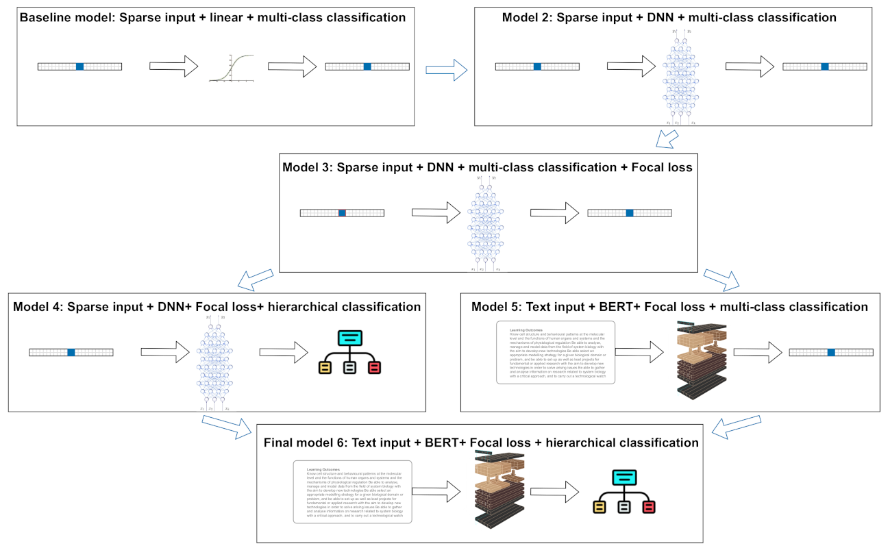
In this study, six models based on the theoretical reasoning described in the section above were constructed. The sequence of proposed models are presented in Figure 1. The mathematical models are described in

Table 1. The elements of proposed mathematical models.

	Input	Model	Output	Loss
1. Baseline	Cat.	Linear	All	${\mathcal{L}}_{CE}$
2. Simple w. CE	Cat.	DNN	All	${\mathcal{L}}_{CE}$
3. Simple w. F	Cat.	DNN	All	${\mathcal{L}}_F$
4. Hier. w. F	Cat.	DNN	Hier.	${\mathcal{L}}_F$
5. Transformer	Text	BERT	All	${\mathcal{L}}_F$
6. Transformer mod.	Text	BERT	Hier.	${\mathcal{L}}_F$

.

Models consist of input data that has either categorical (Cat. in table), i.e., the sparse one-hot representation of given education program, or text (Text in table), i.e., the description of the education program. The architecture of models were build as simple linear, deep feed-forward neural network (DNN) or included transformer neural network (BERT in table). The data output consisted of either all possible classes (All in table) or output of hierarchical classification (Hier. in table). The loss functions were either binary cross-entropy or focal loss. Each model was prepared and tested in the following manner: first, data was prepared and pre-processed, then architecture of model was constructed and training was conducted. Finally, the model performance was evaluated and each model performance was compared against other models. Testing was also performed by applying predictions of models in real-world situations. Each stage of experimentation with models is described in detail in the following sections.

2.3. Data

The experiments were performed on national-level Lithuanian administrative data consisting of information about residents’ acquired education and occupations. The models were created in the Government strategic analysis center of Lithuania (STRATA) within the human resources forecasting project. Only the results of experiments are published in this article.

The data for the training was constructed using several national registers. Data are grouped into 3 main types.

Educational information was retrieved from the register of Education Management Information System (lit. Švietimo valdymo informacinė sistema). Education information consisted of anonymized personal-level data on vocational education, college and university (Bachelor’s, Master’s degree, Integrated studies) studies, and professional education (doctor’s medical practice and pedagogy). There is no equivalent administrative data about doctoral degrees, as for this level of education, unique programs for individual students are composed. Observations consist of education information of graduates or students that achieved graduation (if the education program was not completed, the case was dropped out from the research sample). Education information was additionally translated into English for the textual analysis using Google Cloud Translation API [27].

Educational program abstracts were retrieved from the official and publicly available register, AIKOS, managed by Ministry of Education, Science, and Sport (aprox. 2500 valid programs) [28]. The data was retrieved using scraping tools: Chrome extension Web Scraper [29] and Scrapy [30]. The retrieved information was further processed: translated into English with Google Cloud Translation API [27].

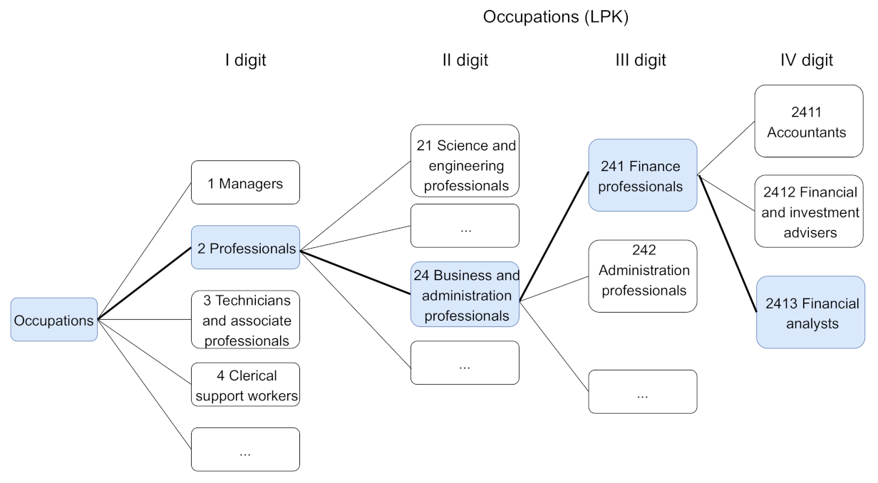
Occupational information was retrieved from The State Social Insurance Fund Board under the Ministry of Social Security and Labour (hereafter abbr. SODRA). Anonymized personal-level occupational data was retrieved for the identified graduates. Occupations were mapped to 4-digit codes according to the Lithuanian version of Standard Classification of Occupations (hereafter abbr. LPK classification) (created in 2012 in accordance to the International Standard Classification of Occupations ISCO-08) [31]. The 4-digit occupational ID has hierarchical structure: first digits branch out into leaves, which branch out further. The first digit represents the status level of the occupation. For example, number “1” represents class of managers and “2”, professionals. The second digit narrows down the speciality of the occupation, for example, “21” represents science and engineering professionals. The third digit shows even more detailed occupational granularity, e.g., “241” signals “Finance professionals”. the fourth digit provides the most detailed information about the occupation, for example, “2411” represents “Accountants”. The number of classes per level are different: the first digit group consists of 10 classes, the second, 43, the third, 130, and the fourth level has 436 classes. Not all classes were observed in the data.

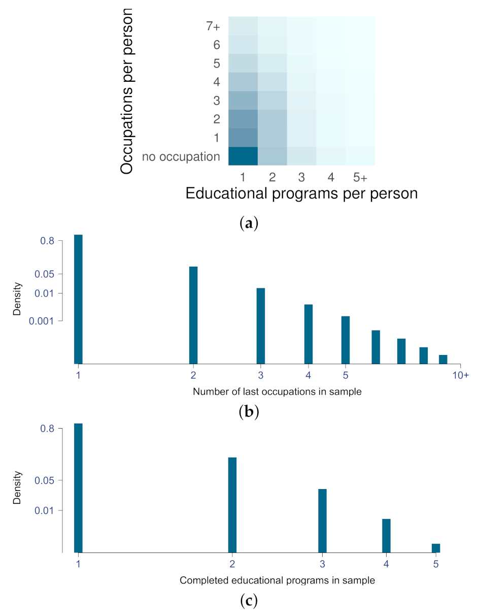
Additional EDA is presented in Figure 2. It is important to note that one person generally completes 1–2 education programs and works one job at any point in time during their career. However, the significant number of cases diverge from general trend and should be accounted during learning process.

Data for the experimentation was constructed as follows: because a single person may have completed multiple education programs with a different number of occupations after and in between education programs, their career timeline is split at education program completion moments into multiple data entries. The sequence of completed education programs per person is combined incrementally starting from first till last education. The sequence of completed programs in each data entry is linked to last occupation in the same time-frame. For example, if a person completed two education programs, we would have two data entries: the first education program linked to the set of last occupation before the second education program was completed, and the input of both; the first and second education programs would be linked to the last occupation after the second education program was completed.

Training, testing and validation sets were split accordingly: 64 percent of data for the training, 16 percent for the validation, 20 percent for the testing set. Thus, for the dataset of 267,201 cases, 171,008 cases were used for the training, 42,752 cases for the validation and 53,441 for the testing.

2.4. Architecture of Experimentation Models

In this study, 6 models were proposed. The summary on layers and parameters of proposed models are presented in

Table 2. Summary of six investigated models. First number (I) indicate the input dimension, the second (P) number present number of learnable parameters in given layer.

Model	Baseline	Model 2	Model 3	Model 4	Model 5	Model 6
Layer type, output shape, param. no.	Input (sparse), I: 2842, P: 0	Input (sparse), I: 2842, P: 0	Input (sparse), I: 2842, P: 0	Input (sparse), I: 2842, P: 0	Input (embedding), I: 768, P: 0	Input (embedding), I: 768, P: 0
	Dense, I:1, P: 2843	Dense, I:1000, P: 2,843,000	Dense, I:1000, P: 2,843,000	Dense, I:1000, P: 2,843,000	Dense, I:1000, P: 76,900	Dense, I:1000, P: 76,900
		Dropout, I:1000, P: 0	Dropout, I:1000, P: 0	Dropout, I:1000, P: 0	Dense, I:1000, P: 1,001,000	Dense, I:1000, P: 1,001,000
	Dense, I:433, P: 866	Dense, I:1000, P: 1,001,000	Dense, I:1000, P: 1,001,000	Dense, I:1000, P: 1,001,000	Dense, I:1000, P: 433,433	Dense, I:1000, P: 1,001,000
		Dropout, I: 1000, P: 0	Dropout, I:1000, P: 0	Dropout, I:1000, P: 0		Concatenate, I:2000, P: 0
		Dense, I:433, P: 433,433	Dense, I: 433, P: 433,433	Dense, I:1000,P: 1001000		Dense, I:1000, P: 2,001,000
				Dropout, I:1000, P: 0		Concatenate, I:3000, P: 0
				Concatenate, I:2000, P: 0		Dense, I:1000, P: 3,001,000
				Dense, I:1000, P: 2,001,000		Concatenate, I:4000, P: 0
				Dropout, I:1000, P: 0		Dense, I: 1000, P: 4,001,000
				Concatenate, 3000, P: 0		Dense, I:9,P: 9009
				Dense, 1000, P: 3,001,000		Dense, I:40, P: 40,040
				Dropout, 1000, P: 0		Dense, I:130, P: 130,130
				Concatenate, 4000,P: 0		Dense, I:433, P: 433,433
				Dense, I:1000, P: 4,001,000
				Dropout, I:1000, P: 0
				Dense, I:9, P: 9009
				Dense, I:40, P: 40,040
				Dense, I:130, P: 130,130
				Dense, I:433, P: 433,433
Total param.	3709	4,277,433	4,277,433	14,460,612	2,203,433	12,386,612

. Models in detail numerical details are described in following subsections.

2.4.1. Baseline, Simple Classification and Simple Classification with Focal Loss Models

For the baseline model input, output layers and 1 hidden layer with 1 neuron were used. Input and output was constructed as one-hot encode representations.

2.4.2. Hierarchical Classification

For the hierarchical model, the data was preprocessed the same way as for simple classification, except for the output data. For the output data, the natural hierarchical structure of occupational code was used, as presented in Figure 3. The data was clustered according to hierarchy of digit in the code (each digit group as separate variable).

2.4.3. Text Embeddings

The descriptions of education programs was used as input text data. Pretrained BERT by Google [32] was used to create text embeddings.

2.4.4. Final Full Model

For the final model, BERT embeddings as input data and output data in hierarchical form was used.

2.5. Text Pre-Processing

The necessity to use such techniques as lemmatization, stemming, removing stop-words, punctuation, etc., before transforming it to embeddings depends on the specific task, data at hand and embedding method. For instance, if context of text is taken into account in the process of embedding, preprocessing methods, such as lemmatization, might violate the parts of the texts that are responsible for the context and thus worsen the transformation. Moreover, the BERT model already contains within its programming library standard forms of text preprocessing [26]. Thus, text was not additionally preprocessed, assuming that procedures within embedding supporting libraries would suffice.

Tokenization is the process where the text is split into number of tokens indexing unique words. BERT for the tokenization uses a vocabulary of 30,522 words. BERT tokenizes not only whole words but also sub-words and this allows us to tokenize articles, expressions or unknowns to dictionary words (to split and use them nonetheless). Maximum length of the accepted sequence is 512 tokens. For longer sequences (for the case of program descriptions using full texts) truncation to the maximum length method was applied. This means too large sequences were truncated token by token, removing a token from the longest sequence in the pair until the proper length is reached. The vector size for each input instance is a length of 768.

2.6. Computational Infrastructure and Complexity

Tensorflow [33] was used as the DNN framework. Each model was trained for 30 epochs. Batch size was set to 256, except for the models with text embeddings 128 batch size was set, as 256 batch size exceeded available computing memory.

All models, except for baseline, were constructed using two fully connected hidden layers. The fully connected layers used ReLu activation function. The output layers used Sigmoid activation function. Selecting the most appropriate number of neurons and other hyperparameters in each different task requires experimentation [34]. For the hyper-parameter tuning, experimentation was performed where per model several settings were tested: number of neurons (100 or 1000) and dropout value (no drop out, 0.1 and 0.5 drop-out). This way, each model was trained 6 times with different hyperparameters.

For the training computer, GPU (Nvidia 1070 ti 8 GB) was used. To use computer memory efficiently, data was stored in sparse matrix form, where nonzero elements are stored as matrix coordinates.

To evaluate models loss, Binary accuracy, Recall, Precision and F1 metrics were used (0.4 threshold was set as maximum probability of predictions because initial experimentation showed that maximum predictions do not reach 0.5).

3. Results and Discussion

3.1. Experimentation

3.1.1. Baseline Model

Loss estimated after 30 epochs—0.014, Binary accuracy—0.998, but Precision, Recall and F1 each had an estimate of 0 (see

Table 3. Results of best performing models on test set. In table different models, the data structure, number of parameters and information about parameters are shown, as well as metrics of Loss, Accuracy (abbr. Acc), Precision (abbr. Pr), Recall (abbr. Re), F1.

Model Name	Units	Drop-Out	Loss	Acc	Pr	Re	F1	Data	Param. No.
Baseline	1	0	0.014	0.998	0.00	0.00	0.00	Sparse	3709
Simple multi-label with Binary crossentr.	1000	0.5	0.012	0.997	0.41	0.13	0.20	Sparse	4,277,433
Simple multi-label with Focal loss	1000	0.5	0.002	0.996	0.22	0.23	0.23	Sparse	4,277,433
Hierarchical classification (default weights)	1000	0.1	0.090					Sparse	14,460,612
I level			0.062	0.859	0.42	0.61	0.50
II level			0.020	0.964	0.35	0.40	0.37
III level			0.007	0.989	0.30	0.26	0.28
IV level			0.002	0.997	0.28	0.19	0.22
BERT embeddings	1000	0	0.002	0.997	0.29	0.16	0.20	Embedd.	2,203,433
Full	1000	0	0.057					Embedd.	12,386,612
I level			0.036	0.856	0.42	0.61	0.49
II level			0.013	0.965	0.35	0.39	0.37
III level			0.006	0.989	0.30	0.24	0.27
IV level			0.002	0.997	0.30	0.16	0.20

). Thus, it is important to note that Binary accuracy metric is not suited for classification task when dealing with large amounts of classes or having an imbalanced training dataset. In this case, if no label is predicted, accuracy is still highly rewarded. The metrics of Precision, Recall and F1 are more informative.

3.1.2. Simple Multilabel Classification with and without Focal Loss

Initial exploratory analysis showed large class imbalance: $\rho$ = 18,041. Moreover, approximately 35 percent of classes do not exceed 100 cases. Therefore, not only was the simple multilabel classification model with Binary cross entropy loss tested but also the model with Focal loss that addresses class imbalance.

The experiments with focal loss showed that $\gamma$ parameter set at three gives the best results. Overall, further analysis of focal loss performance showed that all conditions of hyperparameters achieve better results with Focal loss compared to Binary cross-entropy loss. The results in Table 3 show that Focal loss improves Recall and F1 values by 3 percent in simple multilabel classification task. Regardless of Precision drop, F1 has increased, which can be interpreted as an improvement when using loss regularization. Moreover, experiments with hyperparameters show that the best result is achieved by the two combinations: small number of neurons (100) and medium level of drop-out (0.1) and large number of neurons (1000) with large drop-out. This suggests that for simple multi-label classification tasks, larger and more complex networks tend to over-fit and, therefore, need a larger drop-out value.

For the following models, focal loss as default loss function was applied.

3.1.3. Hierarchical Classification

The exploratory analysis revealed that classes used for the classification task are unbalanced. For example, the largest of first digit (first hierarchical level) LPK occupation set “2” has 128,713 cases (aprox. 49 percent of total cases), and the least number cases belongs to set “6” LPK group with 523 cases. The metrics of class imbalance per level were as follows: for the first digit $\rho =254$, for the second $\rho =3924$, for the third $\rho$ = 22,919, and for the last level, as it was stated previously: $\rho$ = 18,041. Thus, even in the most shallow level, data is extremely unbalanced. Therefore, standard Binary cross-entropy loss was customized, applying $\gamma$ parameter of Focal loss.

As it can be seen from Table 3, hierarchical classification does not improve classification metrics in the most detailed level compared to simple classification model: Recall, Precision and F1 metrics are similar. In shallower levels, F1 scores improves by 6–28 percent. A larger network (1000 neurons per layer) and medium drop-out achieved the best performance.

Despite the inability to improve metrics for accuracy in hierarchical classification, the model predicts smoothly on different levels of output hierarchy. This feature is important for practical applications of the model.

3.1.4. Text Embeddings

The number of parameters in the model with text embeddings, compared to the simple and hierarchical classification models, is smaller. Moreover, the best performing model requires less regularization (the best performing model is with 0 drop-out) as the network type is optimal and tends not to over-fit (see Table 3).

3.1.5. Final Full Model

The final model consisted of BERT text embeddings as input, and a hierarchical structure of occupational classes as output (default weight loss). Full data on the experimentation is presented in Table 3.

All in all, different models performed better than baseline: Recall, Precision and F1 metrics were improved; nevertheless, F1 in the most detailed hierarchy level (433 classes) did not exceed more than 0.30 for all models.

3.2. Applications

In order to better understand how model predictions differ, examples of several education programs were chosen. For the prediction, the best preforming models were used.

Ideally, models should reflect natural frequency in data: occupational distribution of actual data. The final model should predict occupations based on the text description of the program only. Good performance would signal generalization capabilities of the model. The worst case scenario for the model would be the predictions reflecting only the largest classes of occupations for all education programs.

The largest occupational groups in the research dataset are: advertising and marketing professionals (occupational code “2431”)—6 percent of all classes, shop sales assistants (code “5223”)—4 percent of all classes, accountants (code “2411”)—4 percent of all classes, policy administration professionals (code “2422”)—4 percent of all classes.

3.2.1. Investigation of Prediction Capabilities of Different Models

Four examples of education programs (Musical Performance BSc., Modeling and Data Analysis MS., Informatics MS. and Welder vocational training program) were chosen and fitted to different models to predict three occupations with the highest probability. Results were compared with the frequency of occupations given accomplished education.

From

Table A2. Illustrative example of frequencies and Top 3 predictions of all models for the examples of four selected education programs. Outlined in the table the LPK code of occupation, name of the occupation and the probability that the graduate will be employed in the particular occupation.

Model	The Art of Performance, Bachelour dgr.	Modelling and Data Analysis, Master Degree	Informatics, Master Degree	Welder Vocational Training Program
Most frequent occupations of graduates	2652, Musicians, Singers and Composers: 28 %	2631, Economists: 18%	2512, Software Developers: 29%	7212, Welders and Flame Cutters: 9%
	2354, Other Music Teachers: 21 %	2511, Systems Analysts: 15%	2514, Applications Programmers: 17%	5419, Protective Services Workers nec: 6%
	2330, Secondary Education Teachers: 15%	2413, Financial Analysts: 9%	2519, Software, Applications Developers and Analysts nec: 8%	7231, Motor Vehicle Mechanics and Repairers: 5%
Baseline model	2431, Advertising, Marketing Professionals: 0.07	2431, Advertising and Marketing Professionals: 0.07	2431, Advertising, Marketing Professionals: 0.07	2431, Advertising, Marketing Professionals: 0.07
	5223, Shop Sales Assistants: 0.05	5223, Shop Sales Assistants: 0.05	5223, Shop Sales Assistants: 0.05	5223, Shop Sales Assistants: 0.05
	2422, Policy Administration Professionals: 0.04	2422, Policy Administration Professionals: 0.05	2422, Policy Administration Professionals: 0.04	2422, Policy Administration Professionals: 0.05
Simple multilabel with Binary crossentropy	2652, Musicians, Singers and Composers: 0.5	2631, Economists: 0.4	2512, Software Developers: 0.5	7212, Welders and Flame Cutters: 0.7
	2354, Other Music Teachers: 0.2	2413, Financial Analysts: 0.2	2514, Applications Programmers: 0.3	7231, Motor Vehicle Mechanics and Repairers: 0.2
	2330, Secondary Education Teachers: 0.1	2120, Mathematicians, Actuaries, Statisticians: 0.2	2310, University and Higher Education Teachers: 0.2	1221, Sales and Marketing Managers: 0.2
Simple multilabel with Focal loss	2652, Musicians, Singers and Composers: 0.5	2631, Economists: 0.5	2512, Software Developers: 0.5	7212, Welders and Flame Cutters: 0.5
	2354, Other Music Teachers: 0.4	2120, Mathematicians, Actuaries, Statisticians: 0.4	2514, Applications Programmers: 0.4	7516, Tobacco Preparers and Tobacco Products Makers: 0.4
	2330, Secondary Education Teachers: 0.4	2310, University and Higher Education Teachers: 0.4	2310, University and Higher Education Teachers: 0.4	7231, Motor Vehicle Mechanics and Repairers: 0.4
Hierarchical classification Default weights	2, Professionals: 0.5	2, Professionals: 0.6	2, Professionals: 0.6	7, Craft and related trades workers: 0.7
	26, Legal, Social and Cultural Professionals: 0.5	25, ICT Professionals:0.4	25, ICT Professionals: 0.5	72, Metal, machinery, related trades workers: 0.5
	265, Musicians, Singers and Composers: 0.4	251, Software, applications developers and analysts: 0.4	251, Software, applications developers and analysts: 0.5	723, Machinery mechanics and fitters: 0.5
	2652, Musicians, Singers and Composers: 0.5	2631, Economists: 0.4	2512, Software Developers: 0.4	7231, Motor Vehicle Mechanics and Repairers: 0.4
	2354, Other Music Teachers: 0.4	1330, Information and Communications Technology Services Managers: 0.4	2514, Applications Programmers: 0.4	7233, Agricultural and Industrial Machinery Mechanics, Repairers: 0.4
	2659, Creative and Performing Artists Not Elsewhere Classified: 0.4	2512, Software Developers: 0.4	2310, University and Higher Education Teachers: 0.4	7212, Welders and Flame Cutters: 0.3
Word embeddings	2431, Advertising, Marketing Professionals: 0.4	5223, Shop Sales Assistants: 0.4	5223, Shop Sales Assistants: 0.4	2431, Advertising, Marketing Professionals: 0.4
	1219, Business Services and Administration Managers nec: 0.4	2431, Advertising and Marketing Professionals: 0.4	2431, Advertising and Marketing Professionals: 0.3	5223, Shop Sales Assistants: 0.3
	1120, Managing Directors and Chief Executives: 0.4	5419, Protective Services Workers nec: 0.3	5419, Protective Services Workers nec: 0.3	1120, Managing Directors and Chief Executives: 0.3
Universal sentence encoder	2652, Musicians, Singers and Composers: 0.5	2631, Economists: 0.4	2512, Software Developers: 0.5	7212, Welders and Flame Cutters: 0.4
	2354, Other Music Teachers: 0.4	2511, Systems Analysts: 0.4	2514, Applications Programmers: 0.4	7231, Motor Vehicle Mechanics and Repairers: 0.4
	2330, Secondary Education Teachers: 0.4	2413, Financial Analysts: 0.4	2519, Software and Applications Developers and Analysts nec: 0.4	8332, Heavy Truck and Lorry Drivers: 0.4
BERT	2354, Other Music Teachers: 0.4	2631, Economists: 0.5	2512, Software Developers: 0.5	8131, Chemical Products Plant, Machine Operators: 0.4
	5132, Bartenders: 0.4	2120, Mathematicians, Actuaries, Statisticians: 0.4	2514, Applications Programmers: 0.4	7212, Welders and Flame Cutters: 0.4
	5223, Shop Sales Assistants: 0.4	3311, Securities and Finance Dealers and Brokers: 0.4	2513, Web and Multimedia Developers: 0.4	7516, Tobacco Preparers and Tobacco Products Makers: 0.4
Final	2, Professionals: 0.6	2, Professionals: 0.6	2, Professionals: 0.7	7, Craft and related trades workers 0.5
	23, Teaching Professionals: 0.5	25, ICT Professionals: 0.4	25, ICT Professionals: 0.6	72, Metal, machinery, related trades workers: 0.4
	265, Creative and Performing Artists: 0.5	241, Finance Professionals: 0.4	251, Software, applications developers and analysts: 0.5	723, Machinery mechanics and fitters: 0.4
	2652, Musicians, Singers and Composers: 0.5	2631, Economists: 0.4	2514, Applications Programmers: 0.4	7231, Motor Vehicle Mechanics and Repairers: 0.4
	2354, Other Music Teachers: 0.4	2413, Financial Analysts: 0.4	2512, Software Developers: 0.4	9313, Building Construction Labourers: 0.3
	2330, Secondary Education Teachers: 0.4	2511, Systems Analysts: 0.4	2519, Software and Applications Developers and Analysts nec: 0.3	7111, House Builders: 0.3

can be observed that the baseline model performs the worst as it predicts only the largest occupational groups in the data: advertising and marketing professionals, shop sales assistants and policy administration professionals.

Simple multilabel classification models predict more accurately. Both simple models with binary cross-entropy and focal loss perform similarly, except that probability estimates are larger in model with focal loss.

Hierarchical models, as expected, show a tendency to predict in hierarchical order, where the highest probabilities are estimated for the classes of parental hierarchy level and then branches out in accordance with hierarchical structure (in Table A2 only one highest probability for the parental head is shown, yet there could be more classes with similar probabilities).

Models with text embeddings are able to generalize and accurately predict occupation from the text data only.

3.2.2. Prediction of Occupations for Several Education Programs

For practical reasons, it is important that the final model would be able to predict multiple education programs because many graduates complete more than one program.

Table 4. Illustrative example of the final model predictions for several study program combinations.

Informatics, Bachelor dgr.	Informatics, Bachelor and Master dgr.	Informatics, Bachelor dgr, Music Performance, Bachelor dgr.
2, Professionals: 0.6	2, Professionals: 0.7	2, Professionals: 0.6
25, ICT Professionals: 0.6	25, ICT Professionals: 0.5	24, Business and Administration Professionals: 0.4
251, Software and applications developers and analysts: 0.6	251, Software and applications developers and analysts: 0.5	251, Software and applications developers and analysts: 0.4
2514, Applications Programmers: 0.5	2512, Software Developers: 0.4	2512, Software Developers: 0.3
2512, Software Developers: 0.4	2514, Applications Programmers: 0.4	2519, Software and Applications Developers and Analysts nec: 0.3
2519, Software and Applications Developers and Analysts nec: 0.3	2519, Software and Applications Developers and Analysts nec: 0.4	2514, Applications Programmers: 0.3

shows predictions for the different combinations of Informatics studies. It can be seen that for bachelor and master studies, the model predicts similar outcomes.

Examples of mixed education program combinations were also tested. When there are two different education programs of Informatics and Music Performance, the predictions still lead to the ICT occupations with slightly smaller estimated probability values. It is important to note that ICT graduates are one of the most successfully employed groups in Lithuania yet with one of the largest drop-out rates prior to graduation (almost 50 percent do not complete their study program) [35]. Thus, it is possible that the part of the program description related to Informatics education overwhelms the part describing the Music performance.

3.2.3. Prediction of Occupations for New Education Programs

We also tested how the model predicts new programs that some students had already started to study but had not yet graduated (no historical data about occupations). For this exercise, we chose Kaunas University’s newly created (2020) bachelors program “Artificial Intelligence”. The prediction is as follows: for the shallowest level: “2” occupational group named “Professionals” is predicted with 0.7 probability. Then, with the probability 0.5 for the following levels—“25” occupational group or “ICT Professionals” and “251” group “Software and applications developers and analysts” are predicted. The most detailed level is predicted as follows: “2512”, “Software Developers” with 0.4 probability, “2514”, “Applications Programmers” with 0.4 and “2519”, “Software and Applications Developers and Analysts Not Elsewhere Classified” with 0.3 probability. Thus, based on the program description, the model predicts outcomes similarly to those of the Informatics in Vilnius University.

3.2.4. Similarity Search

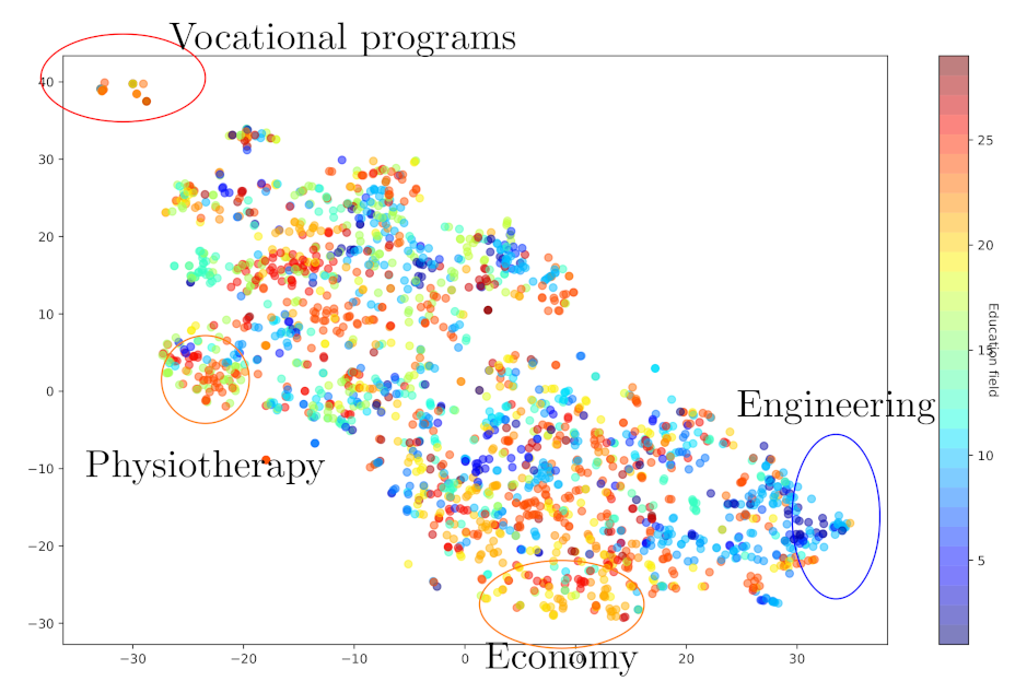
Using high-level features, it is possible to estimate how much the programs are related to each other. High-level features are encoded in the last layers of the deep neural network [36]. In order to investigate the potential usage of the high-level features for similarity search [37], the last layer features of the final model were saved. A similarity search was performed for over 2056 education programs with each program represented by 1000-dimensional feature vector. The t-Distributed Stochastic Neighbor Embedding (abbr. t-SNE) minimizes the divergence between two distributions by measuring pairwise similarities. Corresponding vectors of the high-level feature space were used.

The set of high-level features $\{{\mathbf{f}}_1,{\mathbf{f}}_2,\cdots ,{\mathbf{f}}_N\}$ and Euclidean distance $d({\mathbf{f}}_i,{\mathbf{f}}_j)$ between a pair of objects is used. T-SNE learning an s-dimensional embedding by estimating joint probabilities $p_{ij}$ that measure the pairwise similarity between objects ${\mathbf{f}}_i$ and ${\mathbf{f}}_j$:

$$\begin{array}{cc}\hfill p_{j|i}=\frac{e^{-d{({\mathbf{f}}_i,{\mathbf{f}}_j)}^2/2{\sigma }_i^2}}{{\displaystyle \sum _{k\ne i}{e}^{-d{({\mathbf{f}}_i,{\mathbf{f}}_k)}^2/2{\sigma }_i^2}}},& p_{i|i}=0,p_{ij}=\frac{p_{j|i}+p_{i|j}}{2N}.\end{array}$$

(18)

The visualization of T-SNE for high-level features [38] is demonstrated in Figure 4. The circled groups on the edges of the set visualized in Figure 4 were analyzed in greater detail. These groups cluster into different types of education programs. For example, a program such as mechanical engineering and physiotherapy are displayed on the opposite sides of the set. Similar geometric regularities can be observed for other education types. Related education programs can be identified by relative proximity.

3.2.5. Prediction of Occupations after Program Description Modification

Further analysis of the model’s capability to generalize was performed by altering the education program description. For this task, a vocational program of a Welder training program was chosen. We tested if adding skills to the specific education program would lead to different predictions. The Welder program was supplemented with a set of digital skills.

Table A1. Illustrative example of Final model predictions of pre-modified and post-modified Welder training program description.

Welder Training Program	Welder Training Program Description		ESCO Classification Digital Skills		Welder Training Program with Digital Skills
7, Craft and related trades workers: 0.5	Future metalworking machine operators in theoretical classes are trained in electric and gas welding technologies,		Resolving computer problems, problem- solving with digital tools, digital		7, Craft and related trades workers: 0.5
72, Metal, machinery and related trades workers: 0.4	electric and gas welding equipment, raw material properties and use, electrical engineering, drawing and reading of drawings, preparation of blanks, welding mode		communication and collaboration, using digital tools for collaboration and productivity, analysing and evaluating		74, Electrical and electronic trades workers: 0.4
723, Machinery mechanics and fitters: 0.4	selection, equipment preparation, assembly and welding in various space positions, welded, automatic machines, electric and gas cutting equipment for cutting steel and	+	information and data, digital data processing, software and applications development, analysis, monitoring, inspecting and testing, ICT safety,	=	741, Electrical equipment installers and repairers: 0.4
7231, Motor Vehicle Mechanics and Repairers: 0.4	non-ferrous metals of various profiles, etc. Practical training takes place in school workshops, industrial plants where welding work and metal cutting are performed.		protecting privacy and personal data, developing solutions, managing information, digital content creation, audio-visual techniques		7411, Building and Related Electricians: 0.4
9313, Building Construction Labourers: 0.3	The duration of practical training is 35 weeks. During it, metal welding, drawing and reading of drawings, etc. are consolidated and improved. skills. The welder training		and media production, maintaining and enforcing physical security, complying with envir. protection laws and standards, complying		7212, Welders and Flame Cutters: 0.3
7111, House Builders: 0.3	program is designed for individuals with a secondary education.		HSE procedures, protecting ICT devices, browsing, searching and filtering digital data.		3511, ICT Operations Technicians: 0.3

shows the results of the experiment. Results show that predicted occupations of the altered program are related to the Welder occupation; notably, in some instances, the occupation qualification level is also higher.

4. Conclusions

In this article, the novel application of a transformer neural network for modeling education-to-skill mapping was presented. The final and best performing model is based entirely on the education program description (text input). The model predicts the most probable occupations for program graduates. The model solves the problem of very sparse input data that consists of a large number of study programs and sparse output data with a large number of occupations. The proposed model can produce significantly better results of education-to-skill mapping compared to alternatives using sparse input data. The experiments with focal loss–loss function addressing class imbalance—showed that $\gamma$ parameter can improve model performance. Hierarchical classification allows us to predict the shallower levels of output data hierarchy more accurately. Moreover, shallow levels aggregate classes and, therefore, this feature can be meaningfully employed for practical use. The effectiveness of the proposed model was demonstrated with experiments on national level data, which covers the whole population of Lithuania.

Additional analysis was performed on potential applications of the model and its performance in different settings: applying the model to predict occupations from one or multiple completed education programs, to predict occupations from newly created education programs, to use similarity search among the education programs, and to evaluate the impact of altering the program description.

We have made the code for the proposed network architectures and the interface to predict the occupancy available to the public. The repository can be found online at https://github.com/Stratosfera/education2skill (accessed on 23 June 2021).

References

- Breugel, G.V. Identification and Anticipation of Skill Requirements: Instruments Used by International Institutions and Developed Countries. Project Document. 2017. Available online: https://repositorio.cepal.org/handle/11362/42233 (accessed on 23 June 2021).
- OECD. Skill Measures to Mobilise the Workforce during the COVID-19 Crisis. OECD Policy Responses to Coronavirus (COVID-19). 2020. Available online: https://www.oecd.org/coronavirus/policy-responses/skill-measures-to-mobilise-the-workforce-during-the-covid-19-crisis-afd33a65/ (accessed on 23 June 2021).
- NESTA. Available online: https://www.nesta.org.uk/brief-history-nesta/ (accessed on 18 February 2021).
- CEDEFOP. Available online: https://www.cedefop.europa.eu/ (accessed on 18 February 2021).
- Bamieh, O.; Ziegler, L. How Does the COVID-19 Crisis Affect Labor Demand? An Analysis Using Job Board Data From Austria; Technical Report; Institute of Labor Economics (IZA): Bonn, Germany, 2020. [Google Scholar]
- Lewis, C.; Pain, N. Lessons from OECD forecasts during and after the financial crisis. OECD J. Econ. Stud. 2015, 2014, 9–39. [Google Scholar] [CrossRef] [Green Version]
- Thomas, K.; Hardy, R.D.; Lazrus, H.; Mendez, M.; Orlove, B.; Rivera-Collazo, I.; Roberts, J.T.; Rockman, M.; Warner, B.P.; Winthrop, R. Explaining differential vulnerability to climate change: A social science review. Wiley Interdiscip. Rev. Clim. Chang. 2019, 10, e565. [Google Scholar] [CrossRef] [PubMed] [Green Version]
- An, Z.; Jalles, J.T.; Loungani, P. How well do economists forecast recessions? Int. Financ. 2018, 21, 100–121. [Google Scholar] [CrossRef] [Green Version]
- Makridakis, S.; Hyndman, R.J.; Petropoulos, F. Forecasting in social settings: The state of the art. Int. J. Forecast. 2020, 36, 15–28. [Google Scholar] [CrossRef]
- Zhang, M.L.; Zhou, Z.H. A review on multi-label learning algorithms. IEEE Trans. Knowl. Data Eng. 2013, 26, 1819–1837. [Google Scholar] [CrossRef]
- Goodfellow, I.; Bengio, Y.; Courville, A.; Bengio, Y. Deep Learning; MIT Press: Cambridge, MA, USA, 2016; Volume 1. [Google Scholar]
- Johnson, J.M.; Khoshgoftaar, T.M. Survey on deep learning with class imbalance. J. Big Data 2019, 6, 27. [Google Scholar] [CrossRef]
- Buda, M.; Maki, A.; Mazurowski, M.A. A systematic study of the class imbalance problem in convolutional neural networks. Neural Netw. 2018, 106, 249–259. [Google Scholar] [CrossRef] [PubMed] [Green Version]
- Anand, R.; Mehrotra, K.G.; Mohan, C.K.; Ranka, S. An improved algorithm for neural network classification of imbalanced training sets. IEEE Trans. Neural Netw. 1993, 4, 962–969. [Google Scholar] [CrossRef] [PubMed] [Green Version]
- Mukhoti, J.; Kulharia, V.; Sanyal, A.; Golodetz, S.; Torr, P.H.; Dokania, P.K. Calibrating Deep Neural Networks using Focal Loss. arXiv 2020, arXiv:2002.09437. [Google Scholar]
- Lin, T.Y.; Goyal, P.; Girshick, R.; He, K.; Dollár, P. Focal loss for dense object detection. In Proceedings of the IEEE International Conference on Computer Vision, Venice, Italy, 22–29 October 2017; pp. 2980–2988. [Google Scholar]
- Cerri, R.; Barros, R.C.; De Carvalho, A.C. Hierarchical multi-label classification using local neural networks. J. Comput. Syst. Sci. 2014, 80, 39–56. [Google Scholar] [CrossRef]
- Silla, C.N.; Freitas, A.A. A survey of hierarchical classification across different application domains. Data Min. Knowl. Discov. 2011, 22, 31–72. [Google Scholar] [CrossRef]
- Wang, B.; Wang, A.; Chen, F.; Wang, Y.; Kuo, C.C.J. Evaluating word embedding models: Methods and experimental results. APSIPA Trans. Signal Inf. Process. 2019, 8, e19. [Google Scholar] [CrossRef] [Green Version]
- Kacmajor, M.; Kelleher, J.D. Capturing and measuring thematic relatedness. Lang. Resour. Eval. 2020, 54, 645–682. [Google Scholar] [CrossRef] [Green Version]
- Cer, D.; Yang, Y.; Kong, S.Y.; Hua, N.; Limtiaco, N.; John, R.S.; Constant, N.; Guajardo-Cespedes, M.; Yuan, S.; Tar, C.; et al. Universal sentence encoder. arXiv 2018, arXiv:1803.11175. [Google Scholar]
- Wu, S.; Dredze, M. Beto, bentz, becas: The surprising cross-lingual effectiveness of bert. arXiv 2019, arXiv:1904.09077. [Google Scholar]
- Liu, W.; Wang, Z.; Liu, X.; Zeng, N.; Liu, Y.; Alsaadi, F.E. A survey of deep neural network architectures and their applications. Neurocomputing 2017, 234, 11–26. [Google Scholar] [CrossRef]
- Sutskever, I.; Vinyals, O.; Le, Q.V. Sequence to sequence learning with neural networks. In Proceedings of the Advances in Neural Information Processing Systems, Montreal, QC, Canada, 8–13 December 2014; pp. 3104–3112. [Google Scholar]
- Devlin, J.; Chang, M.W.; Lee, K.; Toutanova, K. Bert: Pre-training of deep bidirectional transformers for language understanding. arXiv 2018, arXiv:1810.04805. [Google Scholar]
- Sun, C.; Qiu, X.; Xu, Y.; Huang, X. How to fine-tune bert for text classification? In China National Conference on Chinese Computational Linguistics; Springer: Berlin/Heidelberg, Germany, 2019; pp. 194–206. [Google Scholar]
- Edmonson, M. GoogleLanguageR: Call Google’s “Natural Language” API, “Cloud Translation” API,“Cloud Speech” API and “Cloud Text-to-Speech”. 2018. Available online: https://rdrr.io/cran/googleLanguageR/ (acessed on 23 June2021).
- AIKOS. Available online: https://www.aikos.smm.lt/Registrai (accessed on 18 February 2021).
- Web Scraper. Available online: https://chrome.google.com/webstore/detail/web-scraper-free-web-scra/jnhgnonknehpejjnehehllkliplmbmhn?hl=en (accessed on 18 February 2021).
- Scrapy. Available online: https://scrapy.org/ (accessed on 18 February 2021).
- LPK. Available online: http://www.profesijuklasifikatorius.lt/?q=en/ (accessed on 18 February 2021).
- Bert-Base-Uncased. Available online: https://huggingface.co/bert-base-uncased (accessed on 18 February 2021).
- Abadi, M.; Barham, P.; Chen, J.; Chen, Z.; Davis, A.; Dean, J.; Devin, M.; Ghemawat, S.; Irving, G.; Isard, M.; et al. Tensorflow: A system for large-scale machine learning. In Proceedings of the 12th USENIX Symposium on Operating Systems Design and Implementation (OSDI 16), Savannah, GA, USA, 2–4 November 2016; pp. 265–283. [Google Scholar]
- Kaastra, I.; Boyd, M. Designing a neural network for forecasting financial. Neurocomputing 1996, 10, 215–236. [Google Scholar] [CrossRef]
- Investuok Lietuvoje, Infobalt, Strata: IRT Specialistai Lietuvoje: Situacija darbo Rinkoje ir Darbdavių Poreikiai. Available online: http://investlithuania.com/wp-content/uploads/2018/03/IRT-specialistai-Lietuvoje.pdf (accessed on 18 February 2021).
- Tishby, N.; Zaslavsky, N. Deep learning and the information bottleneck principle. In Proceedings of the 2015 IEEE Information Theory Workshop (ITW), Jerusalem, Israel, 26 April–1 May 2015; pp. 1–5. [Google Scholar]
- Bell, S.; Bala, K. Learning visual similarity for product design with convolutional neural networks. ACM Trans. Graph. TOG 2015, 34, 1–10. [Google Scholar] [CrossRef]
- T-SNE. Available online: https://pypi.org/project/tsne/ (accessed on 18 February 2021).
Figure 1.
The scheme of six investigated models.
Figure 2.
Diagrams of EDA from top to down: (a) heatmap of completed education and occupational history per person, histograms of (b) occupations and (c) education programs prevalence (on log scale).
Figure 3.
Example of output for hierarchical model for one occupation (code 2431 financial analyst), where larger groups branch out to smaller ones.
Figure 4.
Representation of education programs using t-SNE. Colors indicate larger groups of education field (29 fields in total).