Numerical Quantification of Controllability in the Null Space for Redundant Manipulators

Abstract

Redundant motion, which is possible when robotic manipulators are over-actuated, can be used to control robot arms for a wide range of tasks. One of the best known methods for controlling redundancy is the null space projection, which assigns a priority while executing desired tasks. However, when the manipulator is projected into null space, its motion would be limited, since the motion is only permitted in the direction that does not interfere with the primary task. In this study, we have analyzed the null space projector matrix to derive the appropriate direction of the redundant motion by quantifying the allowed motion in each direction. As a result, we have found an ellipsoidal boundary, in which the redundant motion is permitted to move. We have named this ellipsoidal boundary as ’null space quality’ in directions. The proposed null space quality shows similar aspects with that of the robot manipulability, but it reveals a decisively different value when the manipulator operates within the null space. The experimental results showed that the robotic manipulator tracked the sinusoidal input trajectory with reduced root mean square (RMS) error by 33.84%. Furthermore, we have demonstrated the obstacle avoidance of a robotic arm utilizing the null space projector while considering the null space quality.

1. Introduction

Robot manipulators, which generally consist of six degrees of freedom (DoF), are widely adopted in industrial fields [1]. However, six DoF manipulators can only perform a single task at a single time in three-dimensional space, due to lack of excess DoF. Hence, redundancy is necessary to resolve this issue. Robots are redundant when it has more DoF than the required to perform the given task (e.g., seven DoF for six direction tasks). Redundancy is a crucial feature of robotic manipulators that can be utilized to execute a wide range of tasks with flexibility, dexterity, and versatility. Due to these unique characteristics, redundant manipulators can execute several tasks simultaneously with null space projection [2,3,4]. Applications of null space projection includes, obstacle avoidance [5,6,7], impedance control [8,9,10], the joint saturation [11,12,13], and the posture control [14,15]. Not only does the null space projection enable the robot’s capability to execute tasks simultaneously, it also has the advantage of prioritizing the tasks.

When null space projection is used, excess DoF is utilized to prioritize the tasks into (1) primary task and (2) secondary task. By doing so, the robotic manipulator can execute both tasks simultaneously without disturbing the primary task (higher priority). While executing the tasks, the null space projector plays a key role to minimize the interference. This interference is mainly caused by the multi-DoF dynamics of the robot. Thus, a null space projector was examined with respect to the robot dynamics to stabilize the system [2,16,17]. Although the studies were focused on minimizing the interference of the primary task, a further study must be conducted to consider the controllability of the secondary task.

In the past, numerous studies using self-motion as the secondary task were conducted within the joint space [18,19,20]. However, when the self-motion is conducted within the task space, singularity of robot joints become an issue. Thus, controllability of a robot manipulator must be evaluated while controlling the manipulator within the task space. In a general situation, evaluation of the controllability in task space can be substituted by evaluating the robot manipulability [21]. The robot manipulability refers to the manipulating ability of a robot within the task space, and it is used as an indicator to avoid robot singularity [22]. However, robot manipulability does not account for the changed movable direction of motion due to null space projection. For example, once the null space projector is applied to the robot motion, a new type of singularity occurs. Therefore, a new indicator that deals with this type of singularity is required to evaluate the controllability of a robot within the null space.

In order to address this issue, we propose a new indicator named ’null space quality’, which evaluates the manipulability of a robot with null space projection. Conventional manipulability measures the capacity of a robot to move in a certain direction while considering every single joint. However, it is not possible to evaluate the manipulability in its standard form when the null space projection is used due to the priority of the tasks. This is because the movable direction of motion of a robot changes with the null space projector, in contrast to the movable direction of motion of a robot that considers every single joint. Thus, it is crucial to consider both the null space projector and the Jacobian matrix to deal with the extra capacity of joints.

When the null space projection method is used, it is crucial to consider the controllable direction of a robot. Generally, when the tasks controlled within the null space are under a relatively low DoF situation (i.e., under-actuated), the DoF in task space are usually coupled to one another. Thus, in order to control the robot to the desired motion, it is necessary to find and utilize the controllable direction to acquire better control performance.

The null space quality is a numerical quantification of robot controllability that can be applied universally regardless of the null space projector matrix used. While various null space projectors can be selected depending on the desired task, the null space quality assures a consistent solution for robot control. In this paper, we have introduced a method to obtain the null space quality, while considering both the kinematics and the dynamics of the robots.

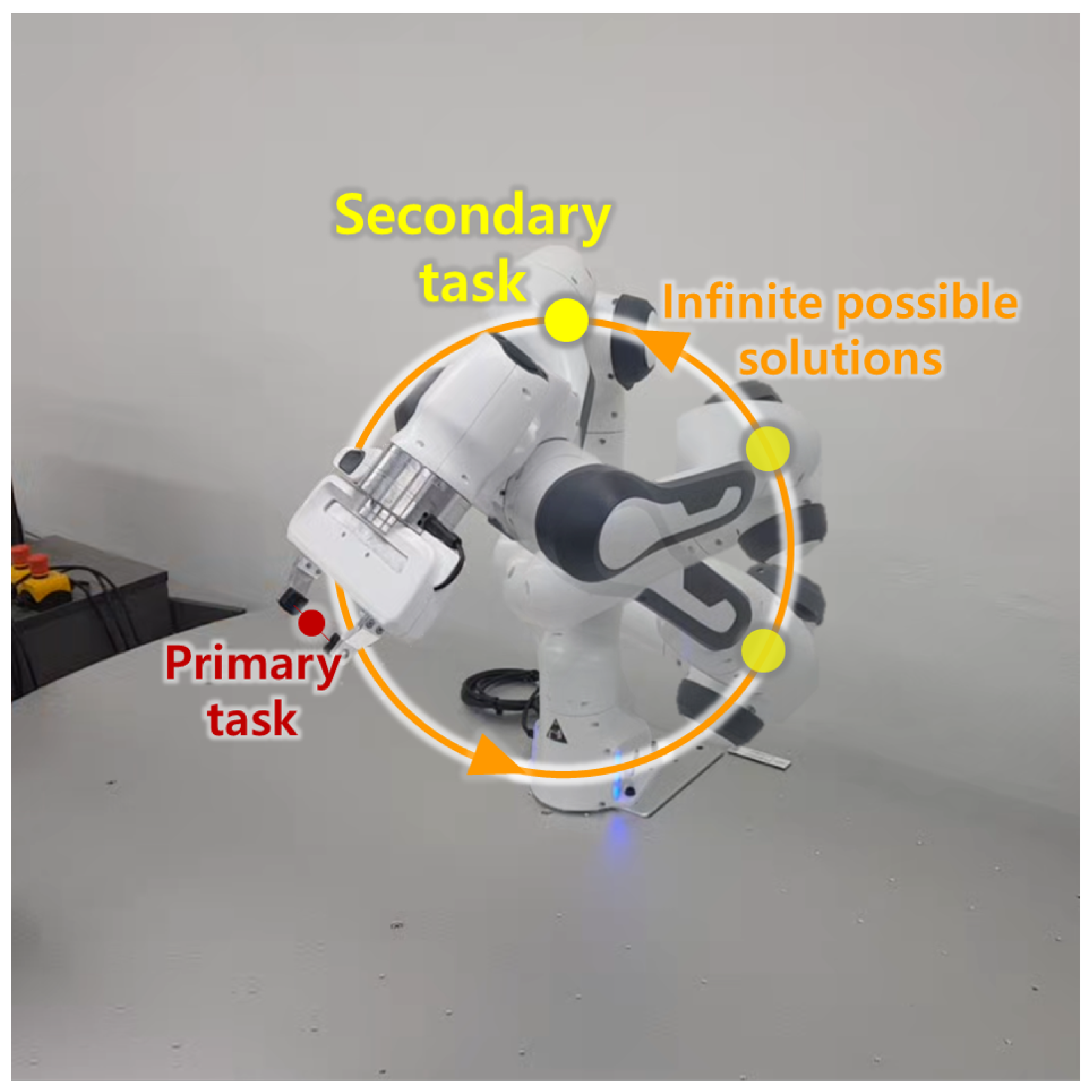
To validate the proposed method, the two tasks were controlled simultaneously. The primary task of a robot is to utilize the six DoF to maintain the end-effector to remain stationary, while the secondary task is to utilize the one DoF at the 4th link to move freely in the direction shown in Figure 1. The infinite number of possible solutions of the secondary task appears in a circular shape because the manipulator is an articulated robot that consists of rotary joints. Hence, the simulation and experiments were performed along the path of the infinitely possible solutions.

2. Method

The manipulator can perform not just a single task, but it can also perform two or more tasks with different priority by using null space projection. For a single task, the relationship between the torque and force is expressed as follows [2]:

$$\Gamma =J^{T}F$$

(1)

where $\Gamma \in R^n$ and $F\in R^m$ denote the torque and the force vector, respectively. $J^T\in R^{n\times m}$ is the Jacobian transpose matrix of the task. If we apply this equation into two simultaneous tasks (e.g., $\Gamma =J_1^T{F}_1+J_2^T{F}_2$), each task will interfere with each other, because the priority of tasks are not assigned to the excess DoF. In order to prioritize the two tasks into primary and secondary tasks simultaneously, without interfering with the primary task, the null space projection should be applied [3]. The corresponding equation of the torque with the null space projection is given in (2):

$$\Gamma =J_P^T{F}_P+N_P^T{J}_S^T{F}_S$$

(2)

$$N_P^T=I-J_P^T{J}_P^{T+}$$

(3)

where $N_P^T\in R^{n\times n}$ and $J_P^{T+}\in R^{m\times n}$ denote the null space projector matrix and Moore–Penrose pseudoinverse matrix of primary task Jacobian transpose, respectively. I is the $n\times n$ identity matrix. The subscripts P and S identifies the primary and the secondary tasks. In this paper, we deal with only two tasks, primary and secondary priorities, but for the general situation, it could be extended further. Based on the Equation (2), the motion generated by the secondary task force, $F_S$, cannot interfere with the motion of the higher priority due to the null space projector $N_P^T$. That is because the null space projector $N_P^T$ constrains the joint motion that is available to $F_S$ due to the assigned priority.

2.1. The Null Space Projector

When using the null space projection for control, the joints of the manipulator move simultaneously in compensation to prevent interference with the high priority task. This compensation acts as a constraint for the secondary task. Thus, finding the controllable joint motion is important. Since the controllable joint motion is the basis vector of the joint space, it is equivalent to the eigenvector of the null space projector. Thus, the eigenvalue decomposition method can be used to acquire an eigenvector. The null space projector consists of the I and $J^T{J}^{T+}$. Because $J^T{J}^{T+}$ is a hermitian matrix with real numbers, and by the definition of the pseudo inverse, the null space projector $N^T$ is always a symmetric matrix. Therefore we can derive the eigenvalues and eigenvectors of the null space projector expressed in the form below:

$$N^T=PD{P}^{-1}(whereP=[P_1\cdots P_k])$$

(4)

The eigenvector $P_i$ is the $n\times 1$ vector and the number of eigenvalue and eigenvector are $k=n-m_P$. $m_P$ is the DoF of primary task. By using these eigenvectors, we can notice the joint constraints and the relationship between each joint while executing the primary task at the end-effector. Furthermore, by projecting the input torque to this eigenvector, we can control the extra joint DoF independently.

$$\Gamma =J_P^T{F}_P+N_P^T{\Gamma }_S$$

(5)

$${\Gamma }_S=K_p{P}_i\frac{P_i·(q_d-q)}{|P_i·(q_d-q)|}|q_d-q|-K_v\dot{q}$$

(6)

Equation (5) shows torque input of a manipulator within the task space, while controlling the joints with null space projector. ${\Gamma }_S$ is the projected torque vector within the eigenvector $P_i$. The vector q and $\dot{q}$ are the vectors representing joint angle and joint angular velocity, respectively. $q_d$ represents the desired joint angle. $K_p$ and $K_v$ are the diagonal matrices containing the proportional and derivative gains, respectively. It is sufficient to perform several tasks like posture control and singularity avoidance by joint space control within the null space, but the tasks like obstacle avoidance, should be performed by task space control even in the null space. We have dealt with this problem in the next section by proposing a new index named null space quality and designating appropriate control direction in the task space.

2.2. Null Space Quality

The ‘null space quality’ is the index that numerically quantifies the manipulating ability of the robot in the null projected task space. In the null space, the controllable direction is changed not only in the joint space, but also in the task space. For enhanced task space control in the null space, it is necessary to identify the controllable direction in the null projected task space. For identification process, the components about the constrained joint motion by null space projector and the manipulating ability of the controlled body should be considered. The null projected Jacobian transpose with respect to the null space projector, $N_P^T$, and Jacobian of the controlled body, $J_S^T$, can be expressed as follows:

$$J_N^T=N_P^T{J}_S^T$$

(7)

The null projected Jacobian contains the relationship between the joint and the task motion in the null space. The relationship can be obtained from the singular values and vectors by the singular value decomposition (SVD) as follow:

$$J_N^T=US{V}^T$$

(8)

where $U\in R^{n\times n}$ and $V\in R^{m\times m}$ are orthogonal unitary matrices involving singular vectors of $J_N^T$, and $S\in R^{n\times m}$ includes singular values, ${\sigma }_i$, in the diagonal. The rank of the $J_N^T$ can be determined as follows:

$$k=\left\{\begin{array}{c}n-m_H\mathrm{if}(n-m_H)\le m_L\hfill \\ m_L\mathrm{if}(n-m_H)>m_L\hfill \end{array}\right.$$

(9)

The relationship between $\delta x$, the infinitesimal displacements of the controlled body, and $\delta q$, the infinitesimal joint angular displacement is defined by $\delta x=J\delta q$. Next, by letting the SVD of Jacobian be $J=V_J{S}_J{U}_J^T$ and substituting it into the equation $\delta x=J\delta q$, the following equation can be derived:

$$\begin{array}{cc}\hfill \delta x& =J\delta q\hfill \\ \hfill & =V_J{S}_J{U}_J^T\delta q\hfill \\ \hfill & =V_J\delta q^{\prime }(where\delta q^{\prime }=S_J{U}_J^T\delta q^{\prime })\hfill \end{array}$$

(10)

In this scope, the matrix $V_J$ and $\delta x$ is expressed in the form of $V_J=[V_{J_1}\cdots V_{J_N}]$ and $\delta x=\delta q_1^{\prime }{V}_{J_1}+\cdots +\delta q_m^{\prime }{V}_{J_m}$. So, the $\delta x$ lies in the column space of $V_J$.

$$\begin{array}{cc}\hfill \delta q& =J^{+}\delta x(where{J}^{+}=U_J{S}_J^{+}{V}_J^T)\hfill \\ \hfill & =U_J{S}_J^{+}{V}_J^T\delta x\hfill \\ \hfill & =U_J\delta x^{\prime }(where\delta x^{\prime }=S_J^{+}{V}_J^T\delta x^{\prime })\hfill \end{array}$$

(11)

By repeating the derivation process above, the $\delta q$ lies in the column space of $U_J$. Based on the equations above, one can note that the U and V in Equation (8) are the basis vectors of the joint space and the task space, respectively. Furthermore, the singular values, ${\sigma }_i$, represent the manipulating abilities of a robot in each direction of the null projected space. Finally, the null space quality can be expressed as:

$$Q=\prod _{i=1}^k{\sigma }_i$$

(12)

The null space quality is the dimensionless index. Since we have used Moore–Penrose pseudoinverse in our work, the null space quality ranges between 0 and 1.0. Generally, high null space quality value interprets the better controllability of the robot manipulator within the null space.

By evaluating the null space quality, another type of singularity can be verified, which cannot simply be verified by evaluating the manipulability. As the null space quality includes the Jacobian matrix, the singular state of the null space quality exhibits similar aspects with the manipulability’s singular state (Type 1 singularity). However, there is a difference due to the null space projector which causes another type of singularity. As mentioned previously, the null space projector restricts the joint motion of a excess Dof, causing singular state. When the constrained joint motion in the null space is orthogonal with the necessary joint motion by the Jacobian, another singular state is caused (Type 2 singularity).

2.3. Null Space Quality Ellipsoid

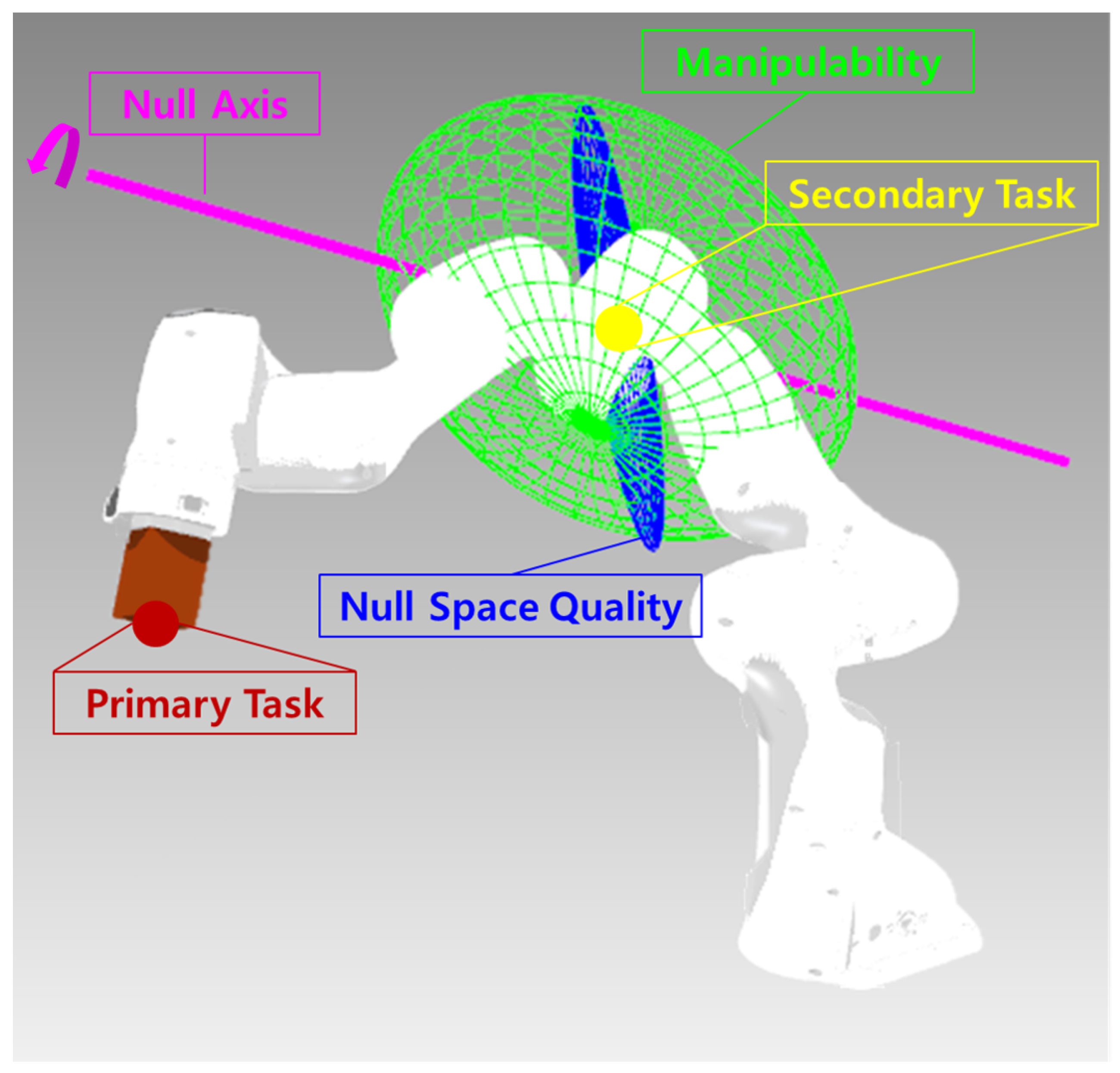
The null space quality ellipsoid, along with the singular values and singular vectors, represents the controllable direction of a robot in the null space. As the null space projected system has relatively low DoF due to the constrained joint motion, the controllable direction and the appropriate force input should be identified. The null space quality ellipsoid could be obtained with the singular values $\sigma$ and the vectors $V_i$ of $J_N^T$ as shown in Figure 2.

$$V=\left[\begin{array}{ccc}{V}_{1_x}& \cdots & V_{k_x}\\ V_{1_y}& \cdots & V_{k_y}\\ V_{1_z}& \cdots & V_{k_z}\\ V_{1_{rx}}& \cdots & V_{k_{rx}}\\ V_{1_{ry}}& \cdots & V_{k_{ry}}\\ V_{1_{rz}}& \cdots & V_{k_{rz}}\end{array}\right]$$

(13)

The column vector $V_i$ represents the controllable DoF in the null projected task space, while the singular values represent the axis length of the ellipsoid. The directional vectors $V_{i_x},V_{i_y}$, and $V_{i_z}$ can be normalized to express the unit vector $V_{i_X}$. By using this ellipsoid, the local solution can be obtained to determine which direction the body may move along, and how the body moves well along that direction. Furthermore, by projecting the force vector to the ellipsoid, the appropriate force can be assigned to the null projected system to improve the control performance.

$$F_L=K_p{V}_{i_X}\frac{V_{i_X}·(x_d-x)}{|V_{i_X}·(x_d-x)|}|x_d-x|-K_v\dot{x}$$

(14)

Next, the null axis that the controlled body may rotate along can be obtained as shown in Figure 2. The articulated manipulator with the constraint can rotate their body along the specified axis. It is important to find the specified axis to predict the direction and the path of the controlled body within the null space. With a rotation term of the singular vector $V_{i_R}$ including $V_{i_{rx}},V_{i_{ry}}$, and $V_{i_{rz}}$, the null axis that the body rotates along can be obtained. For example, the rotation matrix of the null axis $R_N$ using the Roll-Pitch-Yaw method can be obtained from the z-axis as follow:

$$Z^{\prime }=R_{N}Z=\left[\begin{array}{ccc}cos\left(\theta \right)& sin\left(\theta \right)sin\left(\varphi \right)& sin\left(\theta \right)cos\left(\varphi \right)\\ 0& cos\left(\varphi \right)& -sin\left(\varphi \right)\\ -sin\left(\theta \right)& cos\left(\theta \right)sin\left(\varphi \right)& cos\left(\theta \right)cos\left(\varphi \right)\end{array}\right]\left[\begin{array}{c}0\\ 0\\ 1\end{array}\right]$$

$$=\left[\begin{array}{c}sin\left(\theta \right)cos\left(\varphi \right)\\ -sin\left(\varphi \right)\\ cos\left(\theta \right)cos\left(\varphi \right)\end{array}\right]=\left[\begin{array}{c}{V}_{i_{rx}}\\ V_{i_{ry}}\\ V_{i_{rz}}\end{array}\right]$$

$$\varphi =-asin\left(V_{i_{ry}}\right)$$

$$\theta =atan2(V_{i_{rx}},V_{i_{rz}})$$

(15)

$\theta$ and $\varphi$ are the rotation angle in the pitch and yaw direction, respectively. By using (15), the rotation matrix of null axis $R_N$ can be obtained. Based on this method, the null space motion that moves along the null axis can be predicted.

Even though the controllable direction has been identified, the null space projector should be considered. Once the projecting method has been used, the motion of the controlled body remains unchanged, even with or without the null space projector. However, on the joint space level, different joints are activated, which is likely to cause interference to the primary task without the null space projection. Therefore, we have considered the motion of the robot not only in task space level, but also in the joint space level as well.

2.4. Null Space Quality about Dynamic Consistency

The null space quality could apply to the null space projector for other consistencies. For the other consistencies like dynamic [2] and stiffness [23], the null space projector can be changed. Although the joint relationship and limitation are changed by the different null space projectors, the null space quality can be obtained with the same method. So the null space quality could evaluate each null space projector.

The null space projector for dynamic consistency is commonly used to control the redundancy because it guarantees not to interfere with the primary task in both the kinematics level and the dynamics level. The dynamically consistent null space projector ${\overline{N}}_H^T$ is expressed as follows:

$${\overline{N}}_H^T=I-J_H^T{\overline{J}}_H^T$$

(16)

$${\overline{J}}_H=A^{-1}{J}^T\mathsf{\Lambda }$$

$$=A^{-1}{J}^T{\left(J{A}^{-1}{J}^T\right)}^{-1}$$

(17)

${\overline{J}}_H$ is a generalized inverse to minimize the kinetic energy. A is the $n\times n$ joint space kinetic energy matrix. By substituting the ${\overline{N}}_H^T$ to (7) instead of $N_H^T$, the dynamically consistent null projected Jacobian ${\overline{J}}_H$ can be written as:

$${\overline{J}}_N^T={\overline{N}}_H^T{J}_L^T$$

(18)

The null space quality and ellipsoid of ${\overline{J}}_N^T$ can be obtained by the same methods in Section 2.2 and Section 2.3.

3. Simulation and Experiment

To begin with, simulation and experiment were conducted with the 7 DoF robot (PANDA, Franka Emika GmbH, Munchen, Germany ) consisting of the Denavit–Hartenberg parameters shown in

Table 1. The table of the Denavit–Hartenberg parameters for PANDA derived following Craig’s convention, further information on the PANDA can be accessed from the cited link [24].

Joint	a (m)	d (m)	$\mathit{\alpha }$ (rad)	$\mathit{\theta }$ (rad)
Joint 1	0	0.333	0	${\theta }_1$
Joint 2	0	0	$-\frac{\pi }{2}$	${\theta }_2$
Joint 3	0	0.316	$\frac{\pi }{2}$	${\theta }_3$
Joint 4	0.0825	0	$\frac{\pi }{2}$	${\theta }_4$
Joint 5	−0.0825	0.384	$-\frac{\pi }{2}$	${\theta }_5$
Joint 6	0	0	$\frac{\pi }{2}$	${\theta }_6$
Joint 7	0.088	0	$\frac{\pi }{2}$	${\theta }_7$
Flange	0	0.107	0	0

to evaluate the singularities. Then, the simulation was conducted to verify the proposed method by using 6 DoF for the primary task and excess 1 DoF for the secondary task. We compared the general input and the proposed input introduced in Equation (14) to determine the capacity of the projected force input in the proposed method. The magnitude of both force inputs were equal, but the direction differed for each simulation and experiment.

3.1. Types of Singularity

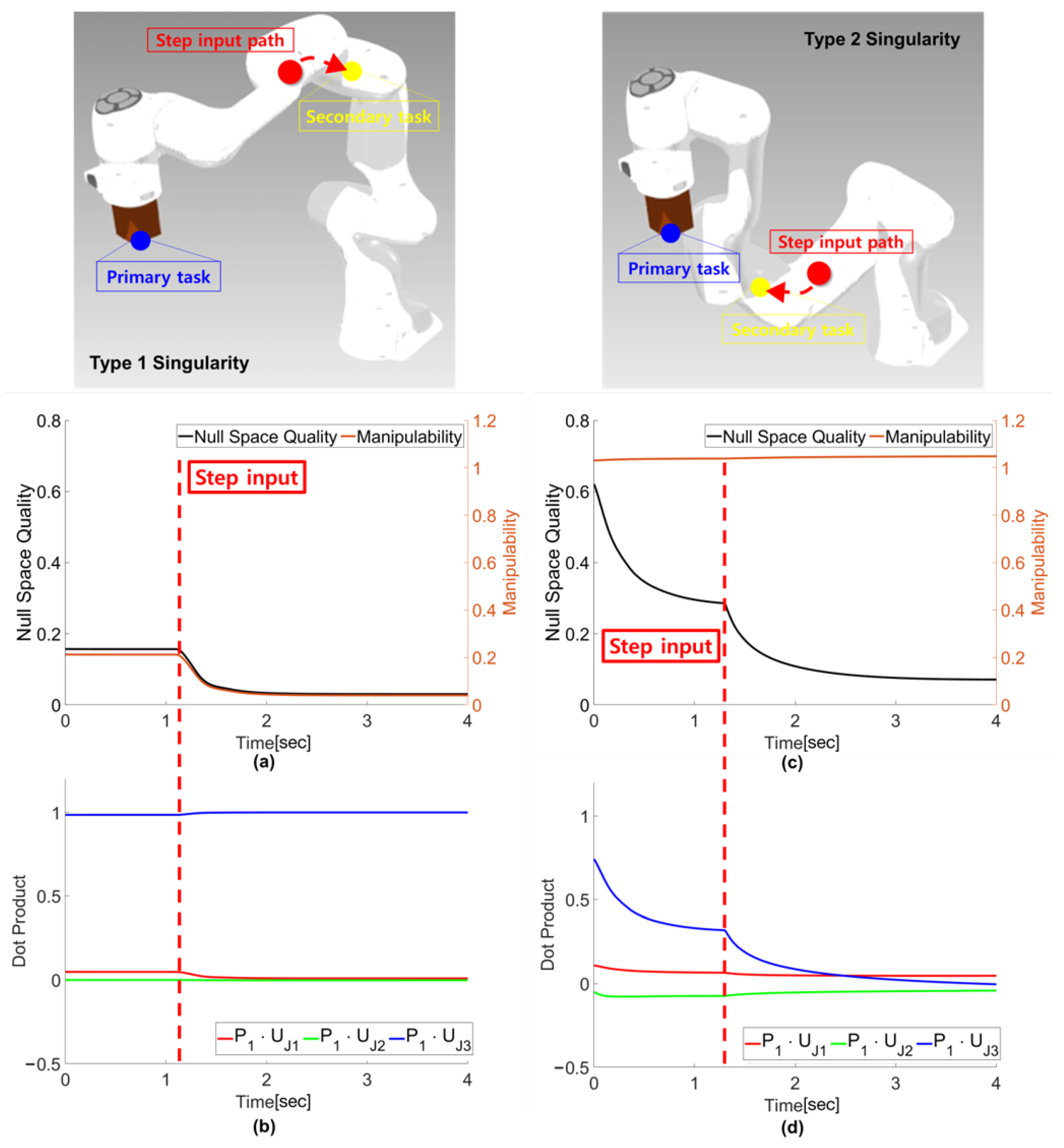
Null space quality can identify two types of singularity, as mentioned at Section 2.2. Type 1 singularity is same as the manipulability because the Jacobian of the control point is dominant in this scope. As shown in Figure 3a, the manipulator moves to the singular configuration with the step input. In this case, both manipulability and null space quality can successfully identify a singular state. This type of singularity can be predicted because it can be determined by the manipulability, which has been studied broadly in the past.

Type 2 singularity appears due to the joint constraint of the robot. Unlike the type 1 singularity, the manipulability remains neutral, while the null space quality decreased with the step input, as shown in Figure 3c. To verify the state, we must obtain the joint vector from the null space projector Jacobian. Three joint bases from the control point’s Jacobian and the dot product with the joint bases of null space projector can be acquired, as shown in Figure 3d. Every dot product of joint vectors is almost orthogonal when the null space quality identifies the singular state. That means every joint vector of the Jacobian is constrained by the null space projector. Thus, a new type of singularity that cannot be explained solely by manipulability can be identified.

3.2. Step and Sinusoidal Response

When controlling the excessive DoF within the null space, there are situations where the desired direction and controllable direction may coincide or differ while disregarding the singular state of the manipulator. In order to validate the proposed method, simulations were conducted to evaluate the response of a robot based on both step and sinusoidal input as shown in Figure 4.

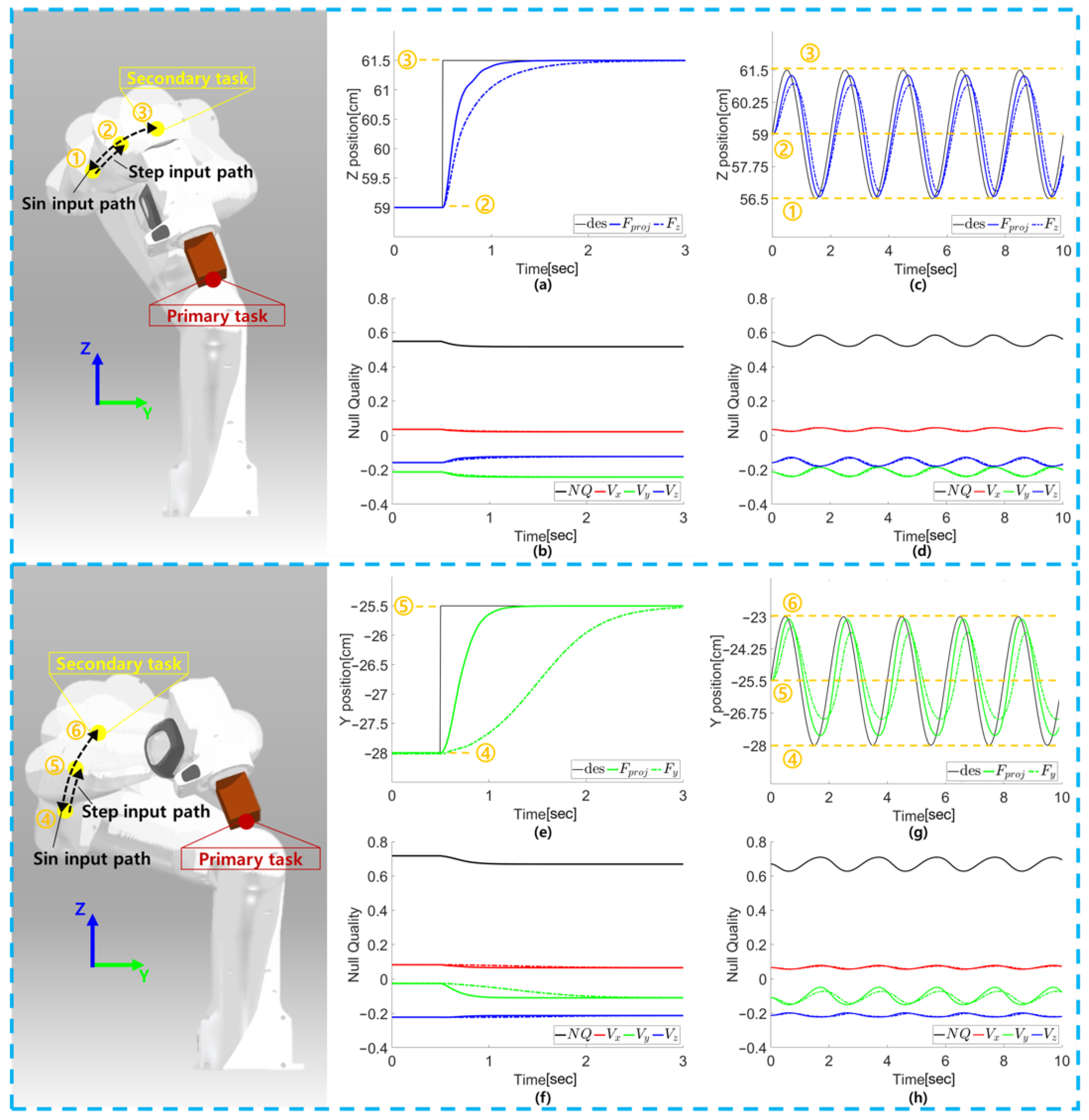
For the first case, both the z-direction input and the proposed input can be controlled with ease (Figure 4a–d). However, the proposed input tends to converge faster, because the proposed input considered the controllable direction in the null space. As shown in Figure 4a, the proposed input converges faster than the z-axis direction input by the reason above. As shown in Figure 4b, the singular vector representing the controllable directions, $V_x$, $V_y$, and $V_z$, changes simultaneously in real-time with respect to the joint configuration of the robot. The resulting motion of a robot with respect to these vectors is shown in Figure 4a. Furthermore, it can be noted that the singular vectors $V_y$ and $V_z$ are relatively larger than the $V_x$, which implies that the robot can be controlled with ease when moving in the y and z directions, but with more difficulty in the x direction. The rise time and the settling time was decreased from 0.6684 [s] to 0.3222 [s] (−51.79%) and from 1.3425 [s] to 0.6061 [s] (−54.82%), respectively. The sine wave input with a cycle per 2 s was simulated as shown in Figure 4c. The RMS error was decreased from 0.0109 [m] to 0.0072 [m] (−33.94%) by using the proposed method.

For comparison, the second case shows the response of a robot moving in the y-direction, even with $V_y$ is low (Figure 4e–h). In Figure 4e, the y position initially cannot follow the desired input, but later follows the desired input as the $V_y$ increases as shown in Figure 4f. Unlike the first case, the control performance can be significantly increased in this case with the proposed force input. The difference here is the force direction, where the proposed input requires greater z-direction than the y-direction at the beginning, as shown in Figure 4f. The rise time and the settling time is decreased from 1.3187 [s] to 0.3497 [s] (−73.48%) and from 2.2736 [s] to 0.6286 [s] (−72.35%), respectively. The sine wave input was simulated as shown in Figure 4g. The results show that the RMS error decreased from 0.0136 [m] to 0.0083 [m] (−38.97%) by using the proposed method.

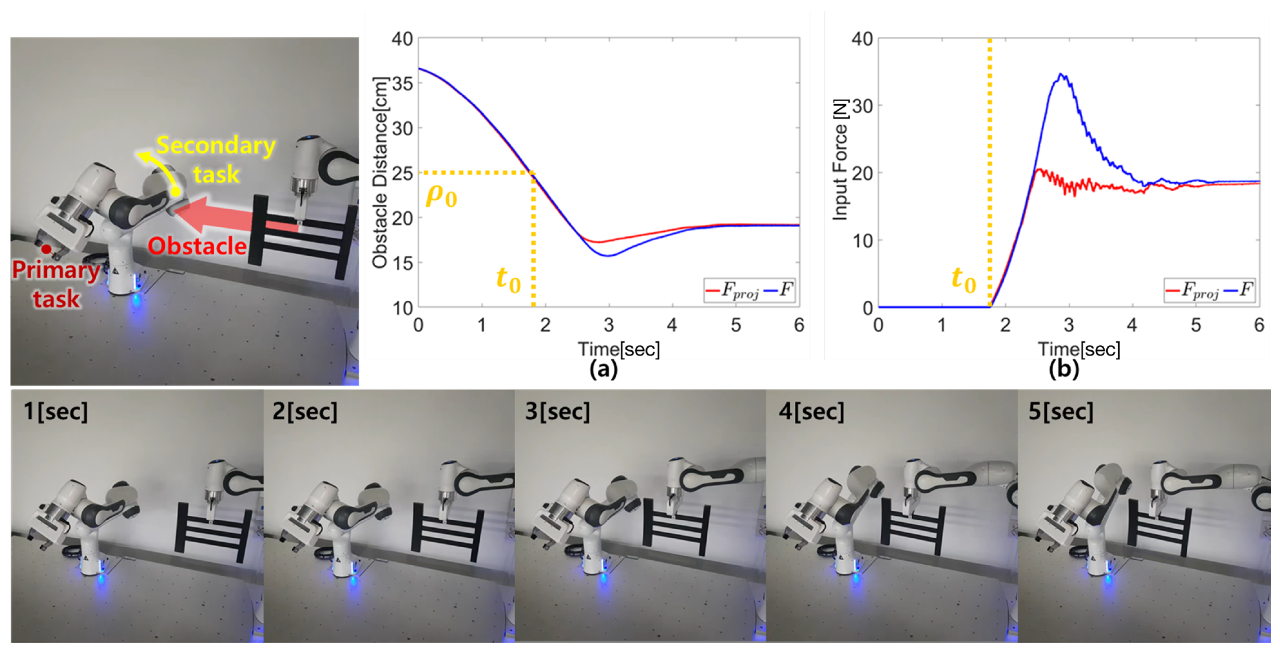
3.3. Obstacle Avoidance

The proposed method can be applied for obstacle avoidance. When obstacle avoidance takes action, it creates a repulsive force with respect to the vector between the robot and the obstacle. When the repulsive force vector points out to an infeasible direction, the manipulator is unable to avoid the obstacle. On the contrary, as the proposed method projects the force to a feasible (movable) direction, the manipulator is able to avoid the obstacle. Even though, the repulsive force points out to a nearby feasible direction, the proposed method can avoid the obstacle with smaller repulsive force with shorter duration.

We have performed obstacle avoidance with the PANDA. The force was selected by a force inducing an artificial repulsion from the surface of the obstacle [25].

$$F_{obs}=\left\{\begin{array}{c}\mu (\frac{1}{\rho }-\frac{1}{{\rho }_0})\frac{1}{{\rho }^2}\frac{\partial \rho }{\partial x}\mathrm{if}\rho \le {\rho }_0,\hfill \\ 0\mathrm{if}\rho >{\rho }_0\hfill \end{array}\right.$$

(19)

The experiment was performed with and without the force projection. With the force projection, the manipulator avoids the obstacle faster with smaller input, as shown in Figure 5. Generally, the magnitude of torque may appear greater or lesser depending on the controllable direction, but when the proposed is used, the magnitude of torque becomes equivalent regardless of the controllable direction.

4. Conclusions

In this paper, we have proposed the index that quantifies the manipulating ability of a robot in the null space. In addition, a novel control method that is more efficient in the null space, especially under low DoF condition, has been proposed. In order to accomplish these contributions, we analyzed the joint constraints caused by the null space projection and the joint and task space basis with respect to the SVD of the null projected Jacobian. Based on these findings, one can find a controllable direction with these bases and control the coupled DoF efficiently by projecting the force to the bases.

We conducted several simulations and experiment to validate the singularity and improved control performances. At the first simulation, the two types of singularity that appear in the null space was verified, one of them which cannot be explained solely with manipulability. We have also conducted simulation to validate the proposed method with respect to the step and sinusoidal input. As a result, the proposed method improved the overall control performance (−51.79% and 73.48% for the rise time, −54.82% and −72.35% for the settling time, −33.94% and −38.97% for RMS error). Furthermore, we applied the proposed method to obstacle avoidance and observed that the task can be performed with a smaller force input with shorter duration of response time for safety.

The null space quality proposed in this work can be a useful substitute for manipulability when we control the null projected system, because it considers the properties of null space that manipulability cannot consider. The proposed control method can be a basic task space control strategy for the null projected system with local optimization. Furthermore, The null space quality can be applied to wide range of applications with regards to the consistency of the projector. In the future, we plan to further enhance the control strategy, so that it can be integrated to redundant robots with more than twp excess DoF.

References

- Almurib, H.A.; Al-Qrimli, H.F.; Kumar, N. A review of application industrial robotic design. In Proceedings of the 2011 Ninth International Conference on ICT and Knowledge Engineering, Bangkok, Thailand, 12–13 January 2012; pp. 105–112. [Google Scholar]
- Khatib, O. A unified approach for motion and force control of robot manipulators: The operational space formulation. IEEE Trans. Robot. Autom. 1987, 3, 43–53. [Google Scholar] [CrossRef] [Green Version]
- Nakamura, Y.; Hanafusa, H.; Yoshikawa, T. Task-priority based redundancy control of robot manipulators. Int. J. Robot. Res. 1987, 6, 3–15. [Google Scholar] [CrossRef]
- Slotine, S.B.; Siciliano, B. A general framework for managing multiple tasks in highly redundant robotic systems. In Proceedings of the 5th International Conference on Advanced Robotics, Pisa, Italy, 19–22 June 1991; Volume 2, pp. 1211–1216. [Google Scholar]
- Maciejewski, A.A.; Klein, C.A. Obstacle avoidance for kinematically redundant manipulators in dynamically varying environments. Int. J. Robot. Res. 1985, 4, 109–117. [Google Scholar] [CrossRef] [Green Version]
- Choi, S.I.; Kim, B.K. Obstacle avoidance control for redundant manipulators using collidability measure. Robotica 2000, 18, 143–151. [Google Scholar] [CrossRef]
- Lee, K.-K.; Buss, M. Obstacle avoidance for redundant robots using Jacobian transpose method. In Proceedings of the International Conference on Intelligent Robots and Systems, San Diego, CA, USA, 29 October–2 November 2007; pp. 3509–3514. [Google Scholar]
- Albu-Schaffer, A.; Ott, C.; Frese, U.; Hirzinger, G. Cartesian impedance control of redundant robots: Recent results with the DLR-light-weight-arms. In Proceedings of the 2003 IEEE International Conference on Robotics and Automation (Cat. No.03CH37422), Taipei, Taiwan, 14–19 September 2003; Volume 3, pp. 3704–3709. [Google Scholar]
- Platt, R.; Abdallah, M.; Wampler, C. Multiple-priority impedance control. In Proceedings of the 2011 IEEE International Conference on Robotics and Automation, Shanghai, China, 9–13 May 2011; pp. 6033–6038. [Google Scholar]
- Sadeghian, H.; Villani, L.; Keshmiri, M.; Siciliano, B. Task-space control of robot manipulators with null-space compliance. IEEE Trans. Robot. 2013, 30, 493–506. [Google Scholar] [CrossRef]
- Flacco, F.; De Luca, A.; Khatib, O. Motion control of redundant robots under joint constraints: Saturation in the null space. In Proceedings of the IEEE International Conference on Robotics and Automation, Saint Paul, MN, USA, 14–18 May 2012; pp. 285–292. [Google Scholar]
- Flacco, F.; De Luca, A.; Khatib, O. Control of redundant robots under hard joint constraints: Saturation in the null space. IEEE Trans. Robot. 2015, 31, 637–654. [Google Scholar] [CrossRef]
- Kanoun, O.; Lamiraux, F.; Wieber, P. Kinematic control of redundant manipulators: Generalizing the task-priority framework to inequality task. IEEE Trans. Robot. 2011, 27, 785–792. [Google Scholar] [CrossRef] [Green Version]
- Bae, J.; Park, J.; Oh, Y.; Kim, D.; Choi, Y.; Yang, W. Task space control considering passive muscle stiffness for redundant robotic arms. Intell. Serv. Robot. 2015, 8, 93–104. [Google Scholar] [CrossRef]
- Khatib, O.; Sentis, L.; Park, J.; Warren, J. Whole-body dynamic behavior and control of human-like robots. Int. J. Humanoid. Robot. 2004, 1, 29–43. [Google Scholar] [CrossRef]
- Park, J. Analysis and Control of Kinematically Redundant Manipulators: An Approach Based on Kinematically Decoupled Joint Space Decomposition. Ph.D. Thesis, Pohang University of Science and Technology, Pohang-si, Korea, 2000. [Google Scholar]
- Wang, J.; Li, Y.; Zhao, X. Inverse kinematics and control of a 7-DOF redundant manipulator based on the closed-loop algorithm. Int. J. Adv. Robot. Syst. 2010, 7, 37–47. [Google Scholar] [CrossRef]
- Tondu, B. A closed-form inverse kinematic modelling of a 7R anthropomorphic upper limb based on a joint parametrization. In Proceedings of the 2006 6th IEEE-RAS International Conference on Humanoid Robots, Genova, Italy, 4–6 December 2006; pp. 390–397. [Google Scholar]
- An, H.H.; Clement, W.I.; Reed, B. Analytical inverse kinematic solution with self-motion constraint for the 7-DOF restore robot arm. In Proceedings of the 2014 IEEE/ASME International Conference on Advanced Intelligent Mechatronics, Besancon, France, 8–11 July 2014; pp. 1325–1330. [Google Scholar]
- Faria, C.; Ferreira, F.; Erlhagen, W.; Monteiro, S.; Bicho, E. Position-based kinematics for 7-DoF serial manipulators with global configuration control, joint limit and singularity avoidance. Mech. Mach. Theory. 2018, 121, 317–334. [Google Scholar] [CrossRef] [Green Version]
- Yoshikawa, T. Manipulability of robotic mechanisms. Int. J. Robot. Res. 1985, 4, 3–9. [Google Scholar] [CrossRef]
- Marani, G.; Kim, J.; Yuh, J.; Chung, W.K. A real-time approach for singularity avoidance in resolved motion rate control of robotic manipulators. In Proceedings of the 2002 IEEE International Conference on Robotics and Automation (Cat. No.02CH37292), Washington, DC, USA, 11–15 May 2002; Volume 2, pp. 1973–1978. [Google Scholar]
- Dietrich, A.; Ott, C.; Albu-Schaffer, A. An overview of null space projections for redundant, torque-controlled robots. Int. J. Robot. Res. 2015, 14, 1385–1400. [Google Scholar] [CrossRef] [Green Version]
- Franka Control Interface Documentation. Available online: Https://frankaemika.github.io/docs/ (accessed on 16 June 2021).
- Khatib, O. Real-time obstacle avoidance for manipulators and mobile robots. Auton. Robot. Veh. 1986, 396–404. [Google Scholar] [CrossRef]
Figure 1.
Actual model of the 7-DoF manipulator. The infinitely possible solutions of the 1-DoF secondary task are shown when performing the positioning and orienting at the end-effector as the primary task.
Figure 2.
The comparison between the manipulability ellipsoid and the null space quality ellipsoid are shown in green and blue, respectively. The null space quality ellipsoid is displayed while controlling 3-DoF (x, y, and z) at the end-effector as a primary task. The controllable ellipsoid of the secondary task is changed from the manipulability ellipsoid to the null space quality ellipsoid by the null space projection. Furthermore, a 1-DoF of the null axis is shown in magenta.
Figure 3.
The two types of singular state configurations are shown. (a) shows the null space quality vs. the manipulability of a manipulator when the manipulator moves to the type 1 singular state by the step input. Type 1 singularity is caused by the Jacobian, which reflects the kinematics of the controlled body. (b) shows the dot product between the joint basis of the null space projector and the Jacobian of the secondary task. The nonzero dot product subset of the joint bases of Jacobian forms the bases after the projection. The dot product is the dimensionless value. (c) shows the type 2 singular state caused by the joint constraints. (d) shows that the dot product of every vector is nearly zero after the step input. This implies that the presence of subset of joint bases that forms the bases in the null space is minimal.
Figure 4.
Simulation results with respect to the step and sinusoidal input are shown. The configuration and movement of the secondary task are described in the left side of the figure. (a–d) are the results when the secondary task is controlled along the z-axis. (a,b) show the response of the robot and the corresponding null space quality when the step input is applied. (c,d) show the response of the robot and the corresponding null space quality when the sinusoidal input is applied. When the desired task is in the z direction, the value of plays a key role. In this situation, is enough to control the robot in the z direction, but the force input projected to V improves the performance. With the step input, the proposed method, which projects the input force into V, decreases the rise time by 51.79% and the settling time by 54.82%. Furthermore, the RMS error has been decreased by 33.94% when the sinusoidal input is applied. (e–h) are the results when the secondary task is controlled along the y-axis. In this case, controlling to y direction is difficult because the , controllability to y direction, is relatively low. In such a situation, the proposed method is more effective. As a result, the rise time, the settling time, and the RMS error decreased by 73.48%, 72.35%, and 38.97%, respectively.
Figure 5.
Experimental results for obstacle avoidance. The schematic of experiment is shown in the left. The primary task is the stationary task by utilizing 6 DoF at the end-effector and the secondary task is obstacle avoidance at link 4 (yellow point) while the obstacle approaches to link 4 from the right side of the manipulator at a speed of 5 cm/s. (a) shows the distance between the obstacle and the control point. (b) shows the input force when the obstacle approaches. is the distance of the obstacle that the manipulator begins to avoid. is the time when the obstacle infiltrates the radius . The proposed method avoids the obstacle faster with the less force input.