
A Method of Defect Depth Recognition in Active Infrared Thermography Based on GRU Networks

School of Mechanical Engineering, Southeast University, Nanjing 211189, China
*
Author to whom correspondence should be addressed.
Appl. Sci. 2021, 11(14), 6387; https://0-doi-org.brum.beds.ac.uk/10.3390/app11146387
Submission received: 26 May 2021
/
Revised: 5 July 2021
/
Accepted: 5 July 2021
/
Published: 10 July 2021
(This article belongs to the Section Computing and Artificial Intelligence)
Abstract
:Active infrared thermography (AIRT) is a significant defect detection and evaluation method in the field of non-destructive testing, on account of the fact that it promptly provides visual information and that the results could be used for quantitative research of defects. At present, the quantitative evaluation of defects is an urgent problem to be solved in this field. In this work, a defect depth recognition method based on gated recurrent unit (GRU) networks is proposed to solve the problem of insufficient accuracy in defect depth recognition. AIRT is applied to obtain the raw thermal sequences of the surface temperature field distribution of the defect specimen. Before training the GRU model, principal component analysis (PCA) is used to reduce the dimension and to eliminate the correlation of the raw datasets. Then, the GRU model is employed to automatically recognize the depth of the defect. The defect depth recognition performance of the proposed method is evaluated through an experiment on polymethyl methacrylate (PMMA) with flat bottom holes. The results indicate that the PCA-processed datasets outperform the raw temperature datasets in model learning when assessing defect depth characteristics. A comparison with the BP network shows that the proposed method has better performance in defect depth recognition.
1. Introduce
Active infrared thermography (AIRT) is widely used in material defect detection by virtue of its visualization and accuracy [1,2]. When the test specimen is subjected to thermal excitation, the irregular inner structure leads to an uneven distribution of the surface temperature field. This phenomenon makes the defect depth determined by AIRT possible. In a study by Vavilov et al., they heated one side of aerospace composites to detect subsurface defects using AIRT [3]. Several non-destructive evaluation (NDE) methods have been applied to deal with thermographic sequences, such as independent component thermography (ICT) [4], pulse phase thermography (PPT) [5], thermographic signal reconstruction (TSR) [6], as well as principal component thermography (PCT) [7,8,9]. In order to eliminate redundant information and reduce computational cost, PCA is adopted in this work to process original temperature datasets.
Quantitative evaluation is a research focus in the field of NDE. Defect information can be detected by peak temperature, peak time, and temperature information at a single moment [10]. Another way to approach defect evaluation is to use deep learning. While it is being widely used in signal processing [11], intelligent control [12], and pattern recognition [13], deep learning also plays an important role in the classification and depth recognition of defect [14,15]. Fang et al. used the finite element method (FEM) and neural networks to evaluate defect depth [16]. Hu et al. proposed a strategy based on long short-term memory (LSTM) networks for the classification of defects [17]. The results demonstrated that deep learning is capable of defect quantitative evaluation. Gated recurrent unit (GRU) is particularly designed for processing temporal sequences to overcome gradient disappearance and explosion in the training and testing process of recurrent neural networks (RNN) [18,19]. Compared with LSTM networks, the GRU networks utilize only a few learning parameters, which improves computational efficiency and can also receive appreciable performance.
In this work, we focus on the defect depth recognition of flat bottom hole defects in polymethyl methacrylate (PMMA) via GRU networks. Halogen lamps are used to heat the PMMA specimen. The thermal response (temperature values change) in the heating and cooling periods is obtained and used as data for the raw temperature datasets. The PCA method is exploited to reconstruct the raw temperature datasets as another principal component datasets. The raw temperature datasets and principal component datasets are used to train and test the GRU model, respectively. The results show that the accuracy of the GRU model trained by principal component datasets is better in defect depth recognition than the model trained by raw temperature datasets. Compared with traditional networks, the GRU model is appealing in processing the thermal sequence.
The rest of this paper is organized as follow: Section 2 describes the theory of active infrared thermography. Section 3 presents the framework of the proposed defect depth recognition method based on the GRU model. Section 4 illustrates the experiment specimen and system. Section 5 provides the results and analysis. Finally, conclusions are given in Section 6.
2. Theory of AIRT
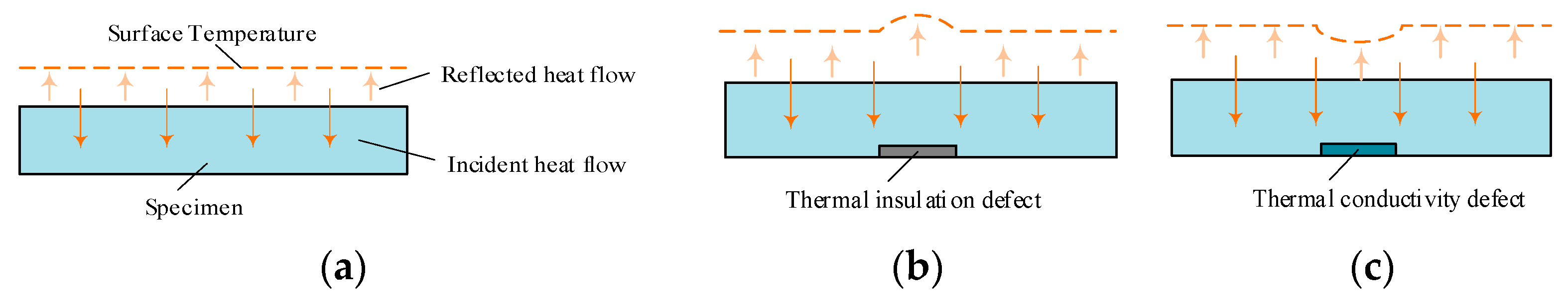
In active infrared thermography (AIRT), a controllable thermal flow is applied to the specimen, and the thermal response is able to be measured during a period of time by an infrared camera [20,21]. The diffusion and transmission of the heat flow are affected when defects exist in the internal structure of the specimen (for example, flat bottom hole defect). This effect will be revealed by the difference in the surface temperature of the specimen before the object reaches thermal equilibrium [22]. Figure 1 illustrates the surface temperature of the specimen under the conditions of existing internal defects and also of without internal defect. The surface temperature distribution of the specimen without defect is showed in Figure 1a. The incident heat flow is partially reflected on the surface of the object; the remaining part continues to diffuse downward; so that a uniform temperature field is formed on the object surface. In Figure 1b, due to the thermal conductivity of the defective region being smaller than that of other regions of the specimen material, the downward transmission of the incident heat flow at the position of defect area is obstructed, and the reflected heat flow is increased; consequently, a relatively hot region is formed on the surface of defect area. On the contrary, it can be seen in Figure 1c that a relatively cold region is formed on the surface of the defective region because of the buried-inside thermal conductivity defect whose thermal conductivity is greater than that of the specimen material.
The surface temperature distribution of the defect region and sound region are different during different periods of time because the inner thermal flow transfer rates of the regions above would influence the surface temperature distribution. The thermal flow transmission in the specimen follows a three-dimensional differential equation of heat conduction, as illustrated below:
where T (K) represents absolute temperature; t (s) indicates the time variable; () is the density of the specimen; C (J/(kg·K)) is the specific heat capacity; (W/(m·K)) are the thermal conductivities for the three respective dimensions in Cartesian coordinates. The specimen exchanges heat with the external fluid and swaps heat with the environment by radiation. The boundary condition is described as:
where n represents normal direction outside the surface, (W/(m·K)) is the main thermal conductivity, the initial environment temperature, h () is heat transfer coefficient, represents surface emissivity, and is the Stefan–Boltzmann radiation constant. The infrared camera obtains the surface temperature distribution of the specimen, and it is a great advantage to use deep learning to determine the defect characteristics using the temperature data.
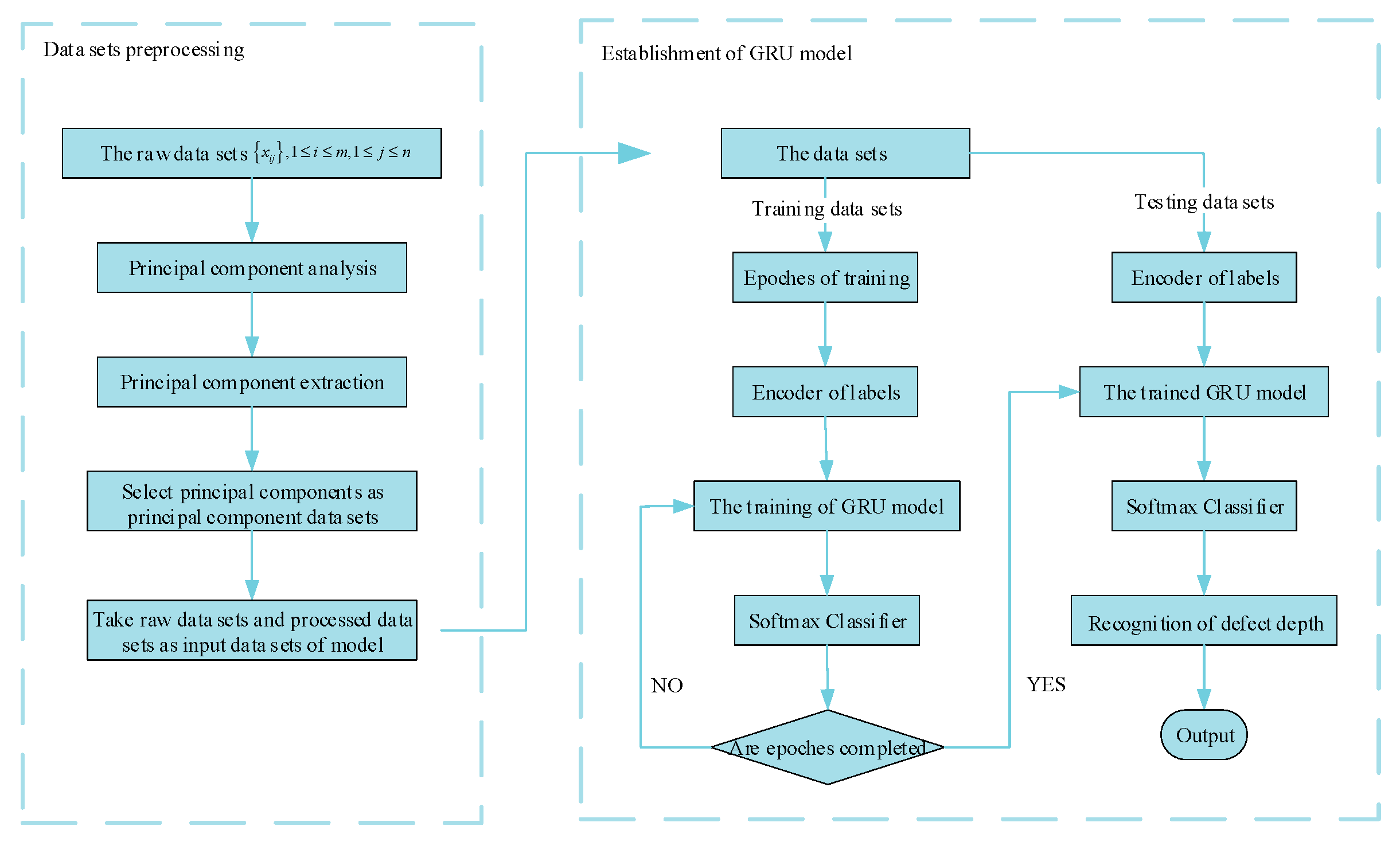
3. Proposed Method for Defect Depth Recognition
Figure 2 illustrates the framework of the proposed defect depth recognition strategy. Two key steps are as follows:
- (1)
- Principal components extraction: The first step is to obtain several irrelevant principal components from the raw thermal sequence that contains redundant information. The procedure of preprocessing the raw thermal sequence by a principal component analysis (PCA) contributes to eliminating correlation and saving the expense of training for network model.
- (2)
- Defect depth recognition based on GRU: The second step is training and testing the GRU model by making the principal components as input datasets to realize defect depth recognition.
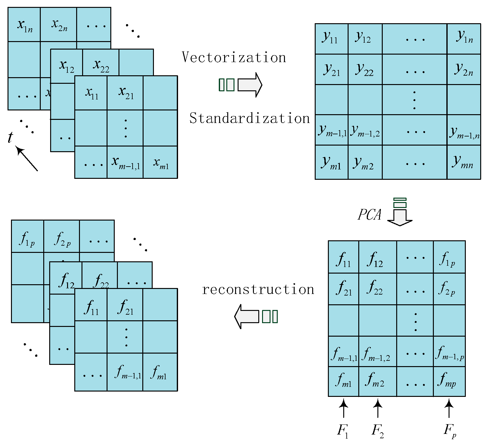
3.1. Principal Components Extraction
After collecting the raw temperature datasets, we used a PCA to decrease the dimension of the datasets above and to reconstruct the uncorrelated principal components as principal component datasets. The procedure of the PCA is indicated in Figure 3.
Assume that raw temperature datasets are reshaped as matrix X, where i represent the number of samples and ranges from 1 to m; j represents the dimension of the raw temperature value and ranges from 1 to n; and represents the temperature value. The matrix X is shown as Equation (3):
Then, the column vector of matrix X is processed by Z-score normalization, and from this we can obtain a new matrix Y. The matrix Y is expressed as follow:
where , , .
We calculate the correlation matrix R of the matrix Y and receive eigenvalues and eigenvectors of matrix R, where , . The first p principal components are formulated as follows:
where p is determined by , .
In the process above, we select the first principal component that contains the most information of the raw temperature datasets as the first index. If cannot fully represent the information of the raw temperature datasets, the second principal component is then selected. We continue this procedure until the major information of the raw temperature datasets is extracted.
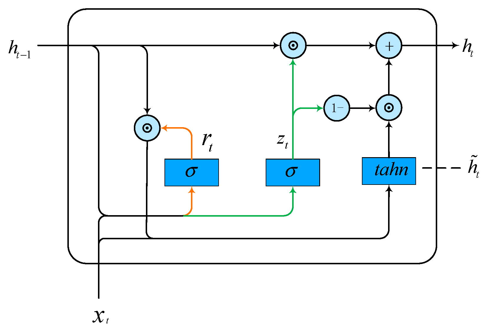
3.2. Defect Depth Recognition Based on GRU
The GRU model is originally from the RNN model, which was designed to specifically process sequence information, such as thermal sequence [23]. The raw temperature datasets processed by PCA were set as principal component datasets; these latter datasets were then fed into the GRU model. The aim here is for the learned GRU model to be able to determine whether the data come from a defective area or a sound area after a period of training.
Compared to long short-term memory (LSTM) networks, the GRU model contains two gate structures, i.e., reset gate and update gate, for the model’s merger of the input gate, the forget gate and the output gate in an LSTM network [24]. The structure of GRU network is depicted in Figure 4, where denotes the input data at current time, represents the hidden state of GRU unit at the current moment, and is the previous hidden state. The function of update gate is to control current input and the previous hidden state , where the value of ranges from 0 to 1. The formulation of is as follows:
where is a sigmoid activation function, and are the update gate weight values, and is the bias.
The function of reset gate determines the influence of the hidden state on the hidden state . Similarly, the value of ranges from 0 to 1; its formulation is as follows:
where and are the reset gate weight values, and is the bias. The calculation for the unit memory information by the update gate is performed as follows:
where is the weight between the input state and the hidden state, is the weight at the hidden state, and is the bias. The output at the current moment is generated as follows:
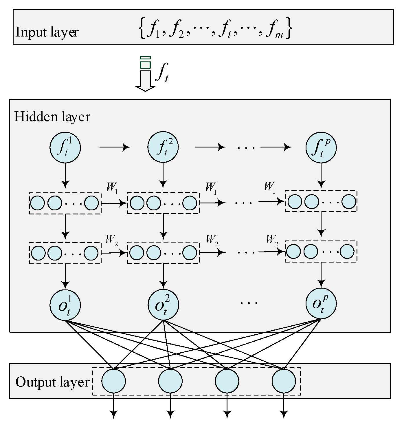
Assume that the principal component datasets are represented as , where i represents the number of samples ranges from 1 to m, and j represents the dimension of the principal component datasets ranges from 1 to p. As shown in Figure 5, the principal component data of sample are fed into the input layer of the GRU model. Each principal component data of the sample from the defect area or sound area is classified with the corresponding defect depth at the output layer of the GRU model based on the depth feature during the period of training. The hidden layer of the network model contains two layers of the GRU, and the weights and of each layer are shared. The output layer contains 4 nodes, and the softmax activation function is applied to recognize whether the sample comes from a defect area or sound area.
4. Experimental Arrangement
4.1. Experimental Specimen
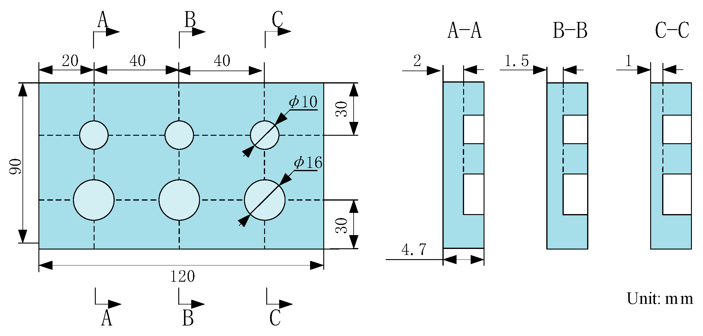
In this work, we chose polymethyl methacrylate (PMMA) as the research object. As shown in Figure 6, the flat bottom hole defects with three different depths were manufactured on the one side of specimen. To verify the adaptability of proposed method, two different diameters were set in manufacturing the defect. The thermal parameters are listed in Table 1.
4.2. Experimental System
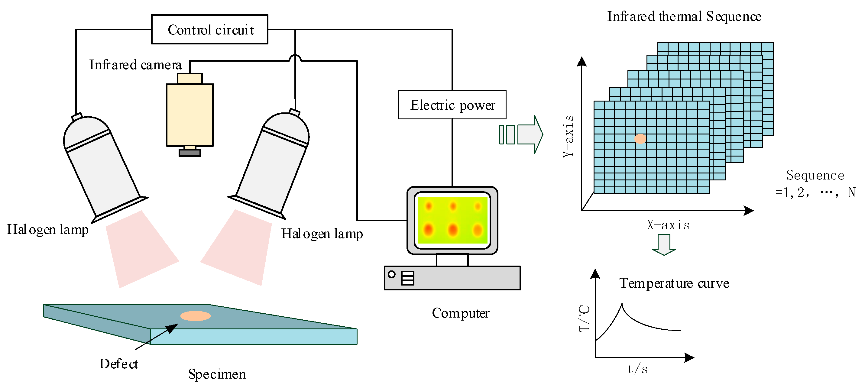
The experimental system set in this work is shown in Figure 7. The excitation source, an infrared camera, a control circuit, and a computer were the main components of the system. We chose two halogen lamps whose power are 1000 W each as the excitation source, and we laid them symmetrically on the non-defective side of the specimen. We used the TiX660 infrared camera (Fluke, USA), whose resolution is 640 × 480 pixel. The control circuit contained time relay and intermediate relay; the function of the former was to control the excitation time, and the latter was to protect the circuit. The computer was connected with the infrared camera by gigabit ethernet to receive and process the datasets collected; the raw datasets were acquired by SmartView software.
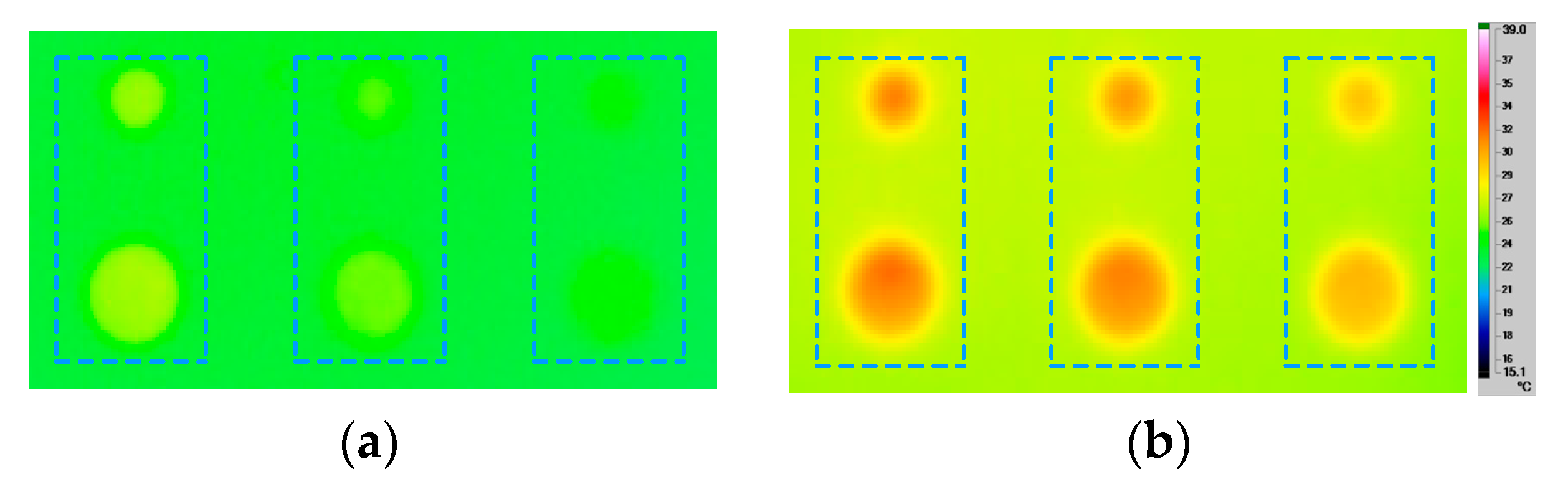
In the experiment, the excitation source and the infrared camera were arranged at the same side of the specimen. The non-defective side of the specimen was heated by halogen lamps for a certain period of time, and then we chilled down the specimen at room temperature. The distance between the specimen and the excitation source was 450 mm, while the distance between the specimen and the infrared camera was 550 mm. The essential parameters of the experiment are listed in Table 2. We collected 90 frames to construct the thermal sequences; the thermal image that represents the specimen surface temperature distribution after 11 s heat excitation is shown in Figure 8a, while Figure 8b represents the thermal image that cooled for 10.5 s at room temperature. From the Figure 8, the surface restricted within respective blue box area shows the visual defects that have the same defect depth, and the defects with different depths had diverse temperature field distributions on the surface.
5. Results and Analysis
5.1. Experimental Data
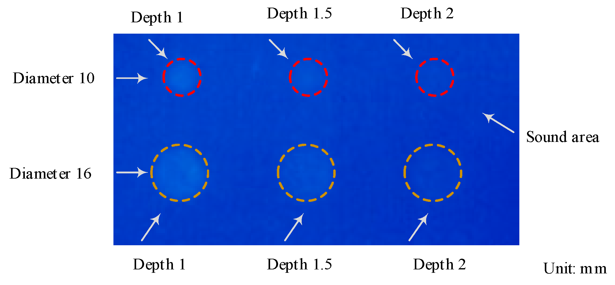
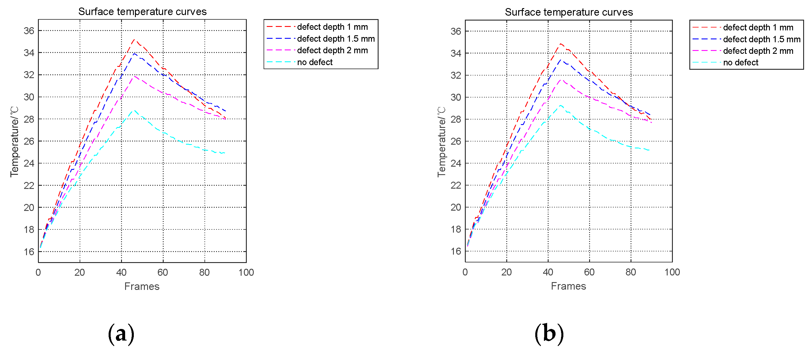
In order to prepare the training and testing data for the GRU model, under the condition of having the same diameter, we divided the non-defective side surface into corresponding areas with three different depths. As shown in Figure 9, the yellow circular areas indicate the three different depth defect areas with a diameter of 16 mm. Similarly, the areas confined within the red circular areas are three different depth defect areas with a diameter of 10 mm. The domain outside the two colored circular areas is the sound area. Under the condition of the two different diameters, we drew four thermal curves that represent the surface temperature of the three different defect areas and the sound areas. As shown in Figure 10, it can be observed that the smaller the defect depth value is, the faster the temperature change rate is. In the three yellow circular areas corresponding to the three depth defect areas and non-defective areas, we selected 180 samples that contain surface temperature change values, respectively, and the operation of vectorization was performed to convert each sample of temperature change value into a two-dimensional raw temperature dataset called R1. Similarly, we selected 180 samples from the three red circular areas and non-defective areas, respectively, and we turned the temperature change values of the samples into another raw temperature dataset called R2. The vectorization above was achieved by stacking each sample temperature change value vector by row.
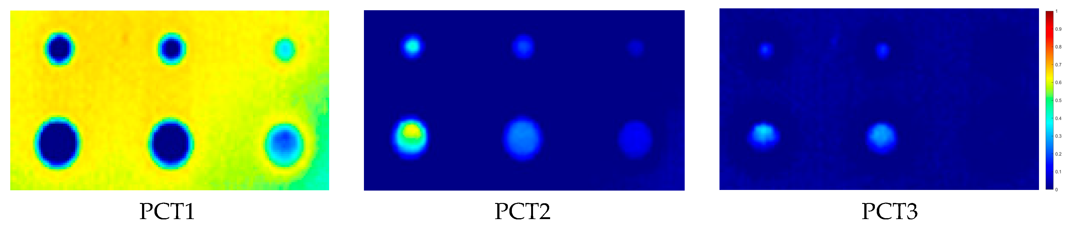
The PCA method was applied to the raw datasets in order to reduce the dimension of the datasets. The raw temperature change values of each pixel were arranged in rows, and the operation of reducing the matrix dimension was carried out by the PCA method. PCT images were obtained by reconstructing the processed matrix in column, and we normalized the contrast of the PCA data. The result processed by the PCA method is depicted in Figure 11; the features of three kinds of defect depth can be clearly observed in PCT1. From PCT2, the defect with depths of 1 mm, 1.5 mm and 2 mm can be fairly easily identified. In addition, the defect features with a depth of 1 mm and 1.5 mm from PCT3 can be effectively distinguished. Due to the of these three principal components being more than 95%, we chose these three components to recognize defect depth. The datasets R1 and R2 that were processed by the PCA method were called M1 and M2, respectively.
5.2. Results Based on GRU Model
The datasets above were divided into training datasets and test datasets by a proportion of 3:7 and then fed into GRU model. The network parameters for the training process were as follows: the Adam optimizer was used to update the weights of the network during the training process; the learning rate was set to 0.001; the time step of the GRU model was set to 3 (3 frames as a time step as input).
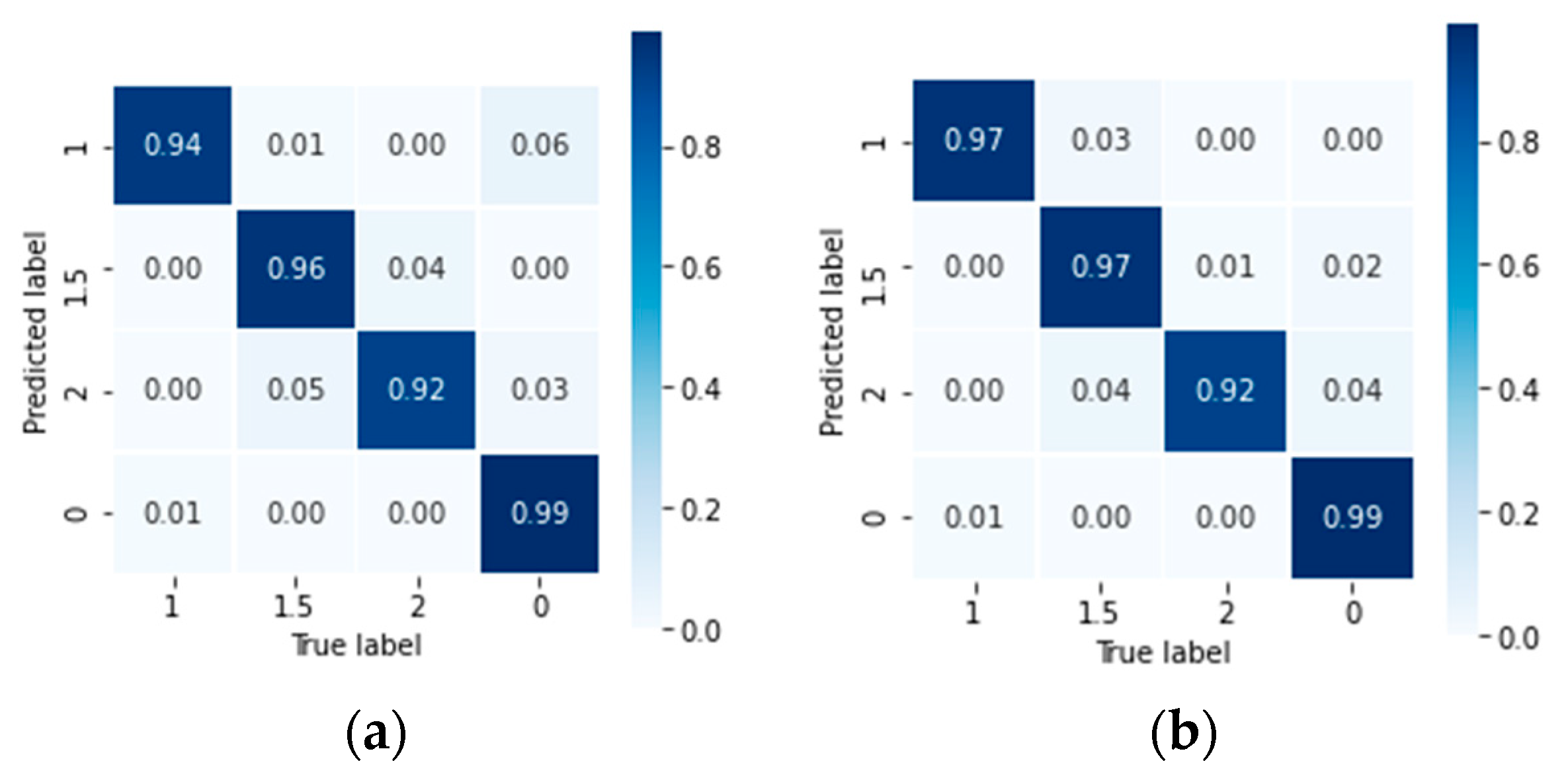
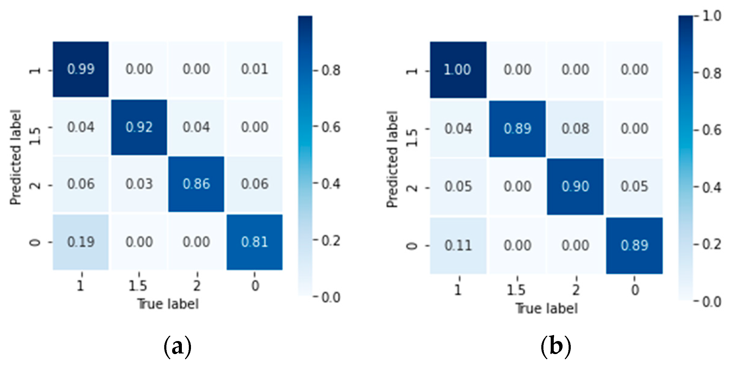
In this work, we used the raw temperature datasets, i.e., R1 and R2, and the respective principal component datasets, i.e., M1 and M2, to train the GRU network. A normalized confusion matrix was applied to assess the performance of the GRU model. In true labels and predicted labels, the number 0 represented the sound areas; the numbers 1, 1.5, and 2 corresponded to the defect depths of 1 mm, 1.5 mm, and 2 mm, respectively. The values on the diagonal of the matrix represented the recall rates of the defect depth recognition, where the recall rates were defined as the proportion of true positive examples that were correctly predicted as positive in the test datasets [25]. As shown in Figure 12, the datasets M1 and M2 obtained a relatively high accuracy in the recognition of the four different defect depths. Under the two diameters conditions, the recognition rate of each defect depth was exceeding 90%. In Figure 13, the recall rates of R1 and R2 were not equal to those of M1 and M2, except the defects with a depth of 1 mm. One possible reason is that the infrared camera was affected by environment noise; this in turn meant that the raw temperature datasets R1 and R2 contained redundant information that contributed to the performance of defect depth recognition, and this is considered undesirable. A summary table that recorded the recall rates regarding the four kinds of datasets is seen in Table 3. The datasets M1 and M2 had higher recall rates in defect depth recognition than datasets R1 and R2 on the whole due to the former eliminating redundant information and strengthening the features of the defect depth. The proposed method did not perform well in the recognition of particular depth defect (e.g., 1 mm); a possible reason is that the samples from the transition region between the defect area and sound area caused the error of recognition.
5.3. Results Based on Traditional Network
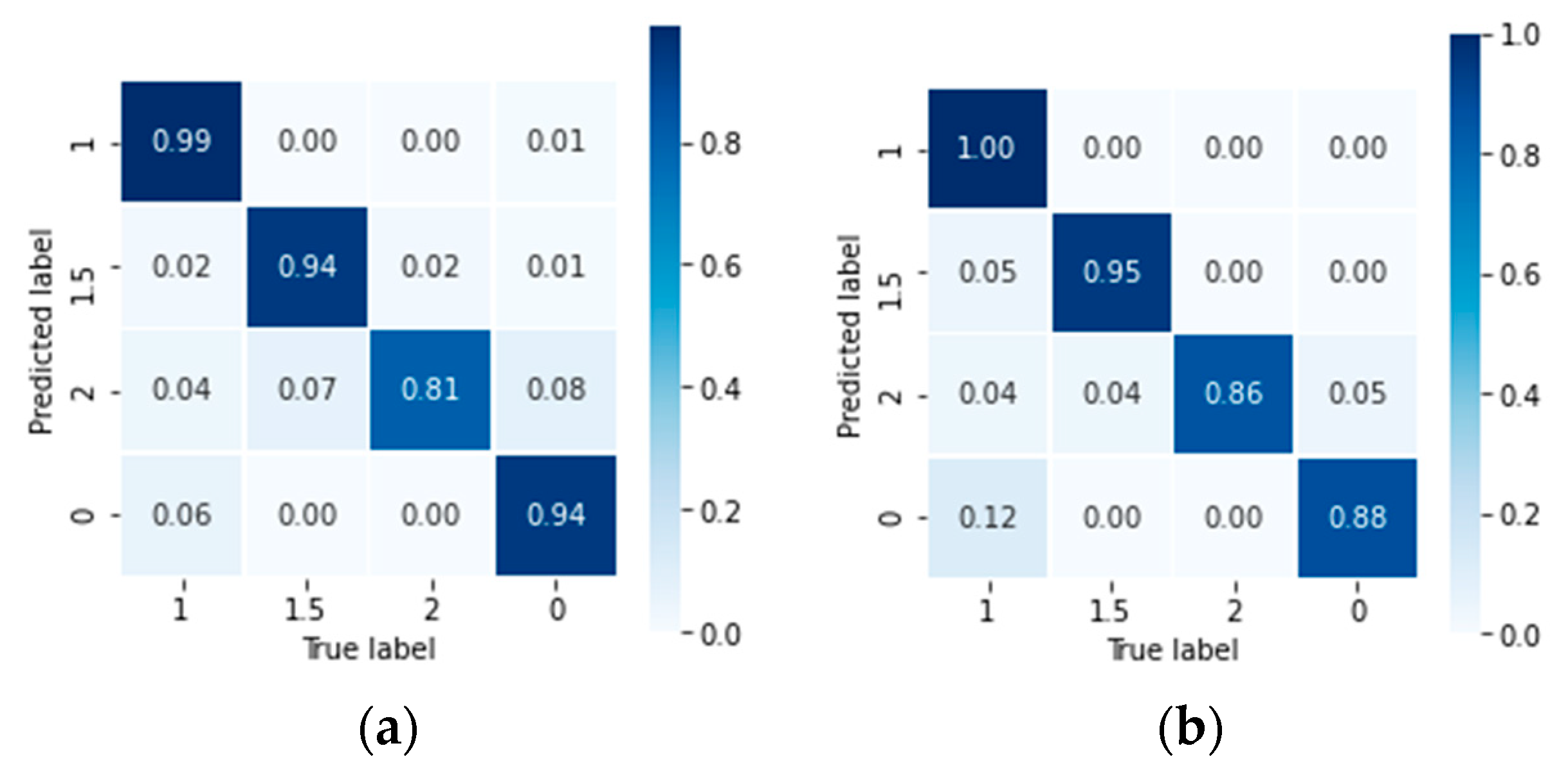
In this work, we used a traditional network trained and tested by datasets M1 and M2 to compare the performance of the GRU model in processing temperature signals. The used widely BP neural network is a classic multilayer feedforward neural network [26]. One hidden layer was set in this model, and the softmax activation function was applied in the output layer to recognize the four types of depth defects. An Adam optimizer was used for updating the weight of the model. The recognition performance of M1 and M2 based on the BP network is shown in Figure 14. The results showed that the recall rates of both datasets were over than 95% under the condition of the depth being 1 mm. In general, the recall rates for depth of 1.5 mm, 2 mm, and sound areas based on the BP model were lower than those of the GRU model. A possible reason is that the GRU network has an advantage over the BP network in processing sequence data, and the former can learn more defect depth features. A summary with the recall rates of M1 and M2 based on the GRU and BP networks is seen in Table 4. In terms of recall rates, the performance of GRU is better than that of BP model, as the former had an advantage in recognizing defect depth.
6. Conclusions
In this paper, we combined the active infrared thermography with the GRU model and PCA to achieve the recognition of the defect depths. The raw datasets obtained by an infrared camera and the datasets processed by PCA were used to verify the performance of the GRU model. PCA is a useful technique for processing thermal sequences by reducing the cost of calculation and eliminating the redundant information. In terms of recall rates, the GRU model trained by principal component datasets had a better performance than the one trained by raw datasets, besides, the former had a faster training speed.
In order to verify the application, defects of two different diameters were set, and the model we proposed proved that it possessed the fairly desirable ability to recognize the defect depths under the condition of the two diameters, respectively. The performance of the GRU model was evaluated by a comparison with the BP neural network; the former performed better than the latter, or in other words, the GRU model was able to learn more defect depth information than the BP model. For the same material, in using AIRT we found that the different defect depths determined the surface thermal response of the defect area. When inspecting a specimen with different plate thicknesses, it is necessary to prepare datasets for the different sound areas.
Improving the quantitative evaluation of defects in non-destructive testing (NDT) is an urgent need, and our work provided a new method for further promoting the application of deep learning in NDT to improve the accuracy of quantitative evaluation. Therefore, the proposed method is a potential candidate for recognizing defect depth.
Author Contributions
L.X. designed and conducted the experiments, proposed the methodology, collected and analyzed the datasets, and wrote the original manuscript; J.H. and L.X. reviewed and edited the manuscript; J.H. provided supervision. Both authors have read and agreed to the published version of the manuscript.
Funding
This research was supported by the National Natural Science Foundation of China (No. 51975117), and Key Research and Development Program of Jiangsu Province (BE2019086).
Institutional Review Board Statement
Not applicable.
Informed Consent Statement
Not applicable.
Data Availability Statement
The data are part of an ongoing project.
Acknowledgments
We would like to thank the school of Mechanical Engineering of the Southeast University. We also thank the Research Center of Condition Monitoring and Fault Diagnosis for academic support.
Conflicts of Interest
The authors declare no conflict of interest.
References
- Ruwandi Fernando, W.D.; Tantrigoda, D.A.; Rosa, S.R.D.; Jayasundara, D.R. Infrared thermography as a non-destructive testing method for adhesively bonded textile structures. Infrared Phys. Technol. 2019, 98, 89–93. [Google Scholar] [CrossRef]
- Wang, Q.; Liu, Q.; Xia, R.; Li, G.; Gao, J.; Zhou, H.; Zhao, B. Defect Depth Determination in Laser Infrared Thermography Based on LSTM-RNN. IEEE Access 2020, 8, 153385–153393. [Google Scholar] [CrossRef]
- Vavilov, V.P.; Pawar, S.S. A novel approach for one-sided thermal nondestructive testing of composites by using infrared thermography. Polym. Test. 2015, 44, 224–233. [Google Scholar] [CrossRef]
- Ahmad, J.; Akula, A.; Mulaveesala, R.; Sardana, H.K. An independent component analysis based approach for frequency modulated thermal wave imaging for subsurface defect detection in steel sample. Infrared Phys. Technol. 2019, 98, 45–54. [Google Scholar] [CrossRef]
- D’Accardi, E.; Palano, F.; Tamborrino, R.; Palumbo, D.; Tatì, A.; Terzi, R.; Galietti, U. Pulsed Phase Thermography Approach for the Characterization of Delaminations in CFRP and Comparison to Phased Array Ultrasonic Testing. J. Nondestruct. Eval. 2019, 38, 1–12. [Google Scholar] [CrossRef]
- Shepard, S.M. Reconstruction and enhancement of active thermographic image sequences. Opt. Eng. 2003, 42, 1337. [Google Scholar] [CrossRef]
- Marinetti, S.; Grinzato, E.; Bison, P.G.; Bozzi, E.; Chimenti, M.; Pieri, G.; Salvetti, O. Statistical analysis of IR thermographic sequences by PCA. Infrared Phys. Technol. 2004, 46, 85–91. [Google Scholar] [CrossRef]
- Cheng, L.; Gao, B.; Tian, G.Y.; Woo, W.L.; Berthiau, G. Impact damage detection and identification using eddy current pulsed thermography through integration of PCA and ICA. IEEE Sens. J. 2014, 14, 1655–1663. [Google Scholar] [CrossRef]
- Rajic, N. Principal component thermography for flaw contrast enhancement and flaw depth characterisation in composite structures. Compos. Struct. 2002, 58, 521–528. [Google Scholar] [CrossRef]
- Zeng, Z.; Li, C.; Tao, N.; Feng, L.; Zhang, C. Depth prediction of non-air interface defect using pulsed thermography. NDT E Int. 2012, 48, 39–45. [Google Scholar] [CrossRef]
- Zhang, S.; Ye, F.; Wang, B.; Habetler, T.G. Semi-Supervised Bearing Fault Diagnosis and Classification using Variational Autoencoder-Based Deep Generative Models. IEEE Sens. J. 2020, 21, 6476–6486. [Google Scholar] [CrossRef]
- Chen, Z.; Liu, Y.; He, W.; Qiao, H.; Ji, H. Adaptive Neural Network-Based Trajectory Tracking Control for a Nonholonomic Wheeled Mobile Robot with Velocity Constraints. IEEE Trans. Ind. Electron. 2020, 68, 5057–5067. [Google Scholar] [CrossRef]
- Pei, J.; Huang, Y.; Huo, W.; Zhang, Y.; Yang, J.; Yeo, T.S. SAR automatic target recognition based on multiview deep learning framework. IEEE Trans. Geosci. Remote Sens. 2018, 56, 2196–2210. [Google Scholar] [CrossRef]
- Duan, Y.; Liu, S.; Hu, C.; Hu, J.; Zhang, H.; Yan, Y.; Tao, N.; Zhang, C.; Maldague, X.; Fang, Q.; et al. Automated defect classification in infrared thermography based on a neural network. NDT E Int. 2019, 107, 102147. [Google Scholar] [CrossRef]
- Darabi, A.; Maldague, X. Neural network based defect detection and depth estimation in TNDE. NDT E Int. 2002, 35, 165–175. [Google Scholar] [CrossRef]
- Fang, Q.; Maldague, X. A method of defect depth estimation for simulated infrared thermography data with deep learning. Appl. Sci. 2020, 10, 6819. [Google Scholar] [CrossRef]
- Hu, C.; Duan, Y.; Liu, S.; Yan, Y.; Tao, N.; Osman, A.; Ibarra-Castanedo, C.; Sfarra, S.; Chen, D.; Zhang, C. LSTM-RNN-based defect classification in honeycomb structures using infrared thermography. Infrared Phys. Technol. 2019, 102, 103032. [Google Scholar] [CrossRef]
- Zhang, X.Y.; Yin, F.; Zhang, Y.M.; Liu, C.L.; Bengio, Y. Drawing and Recognizing Chinese Characters with Recurrent Neural Network. IEEE Trans. Pattern Anal. Mach. Intell. 2018, 40, 849–862. [Google Scholar] [CrossRef] [Green Version]
- Jin, X.B.; Yang, N.X.; Wang, X.Y.; Bai, Y.T.; Su, T.L.; Kong, J.L. Deep hybrid model based on EMD with classification by frequency characteristics for long-term air quality prediction. Mathematics 2020, 8, 214. [Google Scholar] [CrossRef] [Green Version]
- Usamentiaga, R.; Venegas, P.; Guerediaga, J.; Vega, L.; Molleda, J.; Bulnes, F.G. Infrared thermography for temperature measurement and non-destructive testing. Sensors 2014, 14, 12305–12348. [Google Scholar] [CrossRef] [Green Version]
- Chen, D.; Zeng, Z.; Tao, N.; Zhang, C.; Zhang, Z. Liquid ingress recognition in honeycomb structure by pulsed thermography. EPJ Appl. Phys. 2013, 62, 1–8. [Google Scholar] [CrossRef]
- Meola, C.; Boccardi, S.; Carlomagno, G.M. Chapter 4—Nondestructive Testing with Infrared Thermography; Elsevier Ltd.: Amsterdam, The Netherlands, 2017; ISBN 9781782421719. [Google Scholar]
- Dey, R.; Salemt, F.M. Gate-variants of Gated Recurrent Unit (GRU) neural networks. Midwest Symp. Circuits Syst. 2017, 2017, 1597–1600. [Google Scholar] [CrossRef] [Green Version]
- Kanai, S.; Fujiwara, Y.; Iwamura, S. Preventing gradient explosions in gated recurrent units. Adv. Neural Inf. Process. Syst. 2017, 2017, 436–445. [Google Scholar]
- Qu, Y.; Shang, C.; Shen, Q.; Parthaláin, N.M.; Wu, W. Kernel-based Fuzzy-rough Nearest-neighbour Classification for Mammographic Risk Analysis. Int. J. Fuzzy Syst. 2015, 17, 471–483. [Google Scholar] [CrossRef] [Green Version]
- Guo, Z.H.; Wu, J.; Lu, H.Y.; Wang, J.Z. A case study on a hybrid wind speed forecasting method using BP neural network. Knowl. Based Syst. 2011, 24, 1048–1056. [Google Scholar] [CrossRef]
Figure 1.
Surface temperature and heat flow diffusion under different conditions: (a) specimen with no defect; (b) specimen with thermal insulation defect; (c) specimen with thermal conductivity defect.
Figure 1.
Surface temperature and heat flow diffusion under different conditions: (a) specimen with no defect; (b) specimen with thermal insulation defect; (c) specimen with thermal conductivity defect.

Figure 2.
Framework of proposed defect depth recognition strategy.

Figure 3.
Process of PCA.

Figure 4.
The structure of the GRU model.

Figure 5.
The process of depth determination based on GRU.

Figure 6.
The dimension diagram of the specimen.

Figure 7.
The experimental system.

Figure 8.
The temperature field distributions on specimen surface: (a) heated for 11 s; (b) cooled for 10.5 s.
Figure 8.
The temperature field distributions on specimen surface: (a) heated for 11 s; (b) cooled for 10.5 s.

Figure 9.
Schematic diagram of different defect areas.

Figure 10.
Surface temperature curves of different defect depth: (a) diameter is 16 mm; (b) diameter is 10 mm.
Figure 10.
Surface temperature curves of different defect depth: (a) diameter is 16 mm; (b) diameter is 10 mm.

Figure 11.
The result processed by PCA method: PCT1, PCT2, and PCT3.

Figure 12.
The normalized confusion matrix of test datasets from (a) M1; (b) M2.

Figure 13.
The normalized confusion matrix of test datasets from (a) R1; (b) R2.

Figure 14.
The normalized confusion matrix of test datasets from (a) M1 and (b) M2 based on the BP network.
Figure 14.
The normalized confusion matrix of test datasets from (a) M1 and (b) M2 based on the BP network.


Table 1.
The thermal parameters of PMMA and AIR.
| Material | Thermal Conductivity
W/(m·K) | Specific Heat Capacity C J/(kg·K) | Density
kg/m3 |
|---|---|---|---|
| PMMA | 0.18 | 1464 | 1190 |
| AIR | 0.0267 | 1005 | 1.293 |
Table 2.
The parameters of the experiment.
| Heating Power (W) | Heating Time (s) | Cooling Time (s) | Sampling Period (s) |
|---|---|---|---|
| 2000 | 23 | 22 | 0.5 |
Table 3.
The results of defect depth recognition based on the GRU model.
| Datasets | Depth of 1 mm | Depth of 1.5 mm | Depth of 2 mm | Sound Area |
|---|---|---|---|---|
| M1 | 0.94 | 0.96 | 0.92 | 0.99 |
| R1 | 0.99 | 0.92 | 0.86 | 0.81 |
| M2 | 0.97 | 0.97 | 0.92 | 0.99 |
| R2 | 1.00 | 0.89 | 0.90 | 0.89 |
Table 4.
The results of defect depth recognition based on datasets M1 and M2.
| Method | Datasets | Depth of 1 mm | Depth of 1.5 mm | Depth of 2 mm | Sound Area |
|---|---|---|---|---|---|
| GRU | M1 | 0.94 | 0.96 | 0.92 | 0.99 |
| M2 | 0.97 | 0.97 | 0.92 | 0.99 | |
| BP | M1 | 0.99 | 0.94 | 0.81 | 0.94 |
| M2 | 1.00 | 0.95 | 0.86 | 0.88 |
Publisher’s Note: MDPI stays neutral with regard to jurisdictional claims in published maps and institutional affiliations. |
© 2021 by the authors. Licensee MDPI, Basel, Switzerland. This article is an open access article distributed under the terms and conditions of the Creative Commons Attribution (CC BY) license (https://creativecommons.org/licenses/by/4.0/).
Share and Cite
MDPI and ACS Style
Xu, L.; Hu, J. A Method of Defect Depth Recognition in Active Infrared Thermography Based on GRU Networks. Appl. Sci. 2021, 11, 6387. https://0-doi-org.brum.beds.ac.uk/10.3390/app11146387
AMA Style
Xu L, Hu J. A Method of Defect Depth Recognition in Active Infrared Thermography Based on GRU Networks. Applied Sciences. 2021; 11(14):6387. https://0-doi-org.brum.beds.ac.uk/10.3390/app11146387
Chicago/Turabian StyleXu, Li, and Jianzhong Hu. 2021. "A Method of Defect Depth Recognition in Active Infrared Thermography Based on GRU Networks" Applied Sciences 11, no. 14: 6387. https://0-doi-org.brum.beds.ac.uk/10.3390/app11146387
Note that from the first issue of 2016, this journal uses article numbers instead of page numbers. See further details here.