Kernel-Based Phase Transfer Entropy with Enhanced Feature Relevance Analysis for Brain Computer Interfaces

Abstract

Neural oscillations are present in the brain at different spatial and temporal scales, and they are linked to several cognitive functions. Furthermore, the information carried by their phases is fundamental for the coordination of anatomically distributed processing in the brain. The concept of phase transfer entropy refers to an information theory-based measure of directed connectivity among neural oscillations that allows studying such distributed processes. Phase TE is commonly obtained from probability estimations carried out over data from multiple trials, which bars its use as a characterization strategy in brain–computer interfaces. In this work, we propose a novel methodology to estimate TE between single pairs of instantaneous phase time series. Our approach combines a kernel-based TE estimator defined in terms of Renyi’s $\alpha$ entropy, which sidesteps the need for probability distribution computation with phase time series obtained by complex filtering the neural signals. Besides, a kernel-alignment-based relevance analysis is added to highlight relevant features from effective connectivity-based representation supporting further classification stages in EEG-based brain–computer interface systems. Our proposal is tested on simulated coupled data and two publicly available databases containing EEG signals recorded under motor imagery and visual working memory paradigms. Attained results demonstrate how the introduced effective connectivity succeeds in detecting the interactions present in the data for the former, with statistically significant results around the frequencies of interest. It also reflects differences in coupling strength, is robust to realistic noise and signal mixing levels, and captures bidirectional interactions of localized frequency content. Obtained results for the motor imagery and working memory databases show that our approach, combined with the relevance analysis strategy, codes discriminant spatial and frequency-dependent patterns for the different conditions in each experimental paradigm, with classification performances that do well in comparison with those of alternative methods of similar nature.

1. Introduction

Neural oscillations are observed in the mammalian brain at different temporal and spatial scales [1]. Oscillations in specific frequency bands are present in distinct neural networks, and their interactions have been linked to fundamental cognitive processes such as attention and memory [2,3] and to information processing at large [4]. Three properties characterize such oscillations: amplitude, frequency, and phase, the latter referring to the position of a signal within an oscillation cycle [5]. Oscillation amplitudes are related to neural synchrony expansion in a local assembly, while the relationships between the phases of neural oscillations, such as phase synchronization, are involved in the coordination of anatomically distributed processing [6]. Moreover, from a functional perspective, phase synchronization and amplitude correlations are independent phenomena [7], hence the interest in studying phase-based interactions independently from other spectral relationships. Additionally, phase relationships are linked to neural synchronization and information flow within networks of connected neural assemblies [8]. Therefore, a measure that aims to capture phase-based interactions among signals from distributed brain regions should ideally include a description of the direction of interaction. A fitting framework for such measure is that of brain effective connectivity [9].

Effective brain connectivity, also known as directed functional connectivity, measures the influence that a neural assembly has over another one, establishing a direction for their interaction by estimating statistical causation from their signals [10]. Directed interactions between oscillations of similar frequency can be captured through measures such as Geweke-Granger causality statistics, partially directed coherence, and directed transfer function [9,11]. However, since these metrics depend on both amplitude and phase signal components, they do not identify phase-specific information flow [8]. The phase slope index (PSI), introduced in [12], measures the direction of coupling between oscillations from the slope of their phases; still, it only captures linear phase relationships [13]. In this context arises the concept of phase transfer entropy, a phase-specific nonlinear directed connectivity measure introduced in [8]. Transfer entropy (TE) is an information-theoretic quantity, based on Wiener’s definition of causality, that estimates the directed interaction, or information flow, between two dynamical systems [14,15]. In [8], the authors first extract instantaneous phase time series by complex filtering the signals of interest in a particular frequency, since a signal’s phase is only physically meaningful when its spectrum is narrow-banded [16]. Such filtering-based approach has also been explored to obtain phase-specific versions of other information-theoretic metrics such as permutation entropy and time-delayed mutual information [7,16]. Then, the authors compute TE from the obtained phase time series. Nonetheless, since conventional TE estimators are not well suited for periodical variables, in [8] phase TE estimates are obtained through a binning approach performed over multiple trials simultaneously, in a procedure termed trial collapsing.

Phase TE has found multiple applications in neuroscience, such as gaining insight into reduced levels of consciousness by evaluating brain connectivity [17], analyzing resting-state networks [18], and assessing brain connectivity changes in children diagnosed with attention deficit hyperactivity disorder following neurofeedback training [19]. It has even been used to detect fluctuations in financial markets data [20]. Nonetheless, phase TE, estimated as in [8], cannot be employed as a characterization strategy for brain–computer interfaces (BCI) since they require features extracted on an independent trial basis, i.e., each trial must be associated with a set of features. Effective connectivity measures, such as phase TE, can be used to assess the induced physiological variations in the brain occurring during BCI tasks [21]. Discriminative information may be hidden in the dynamical interactions among spatially separated brain regions that characterization methods commonly employed in BCI are not able detect [22]. This information could be relevant to address issues such as the inefficiency problem in some BCI systems [23]. In that context, authors in [6] applied a binning strategy to estimate single-trial phase TE to set up classification systems for visual attention. Nonetheless, binning estimators for single trial-based estimation of information-theoretic measures exhibit systematic bias [8]. Furthermore, spectrally resolved TE estimation methods that can obtain single-trial TE estimates have been recently proposed in the literature [24,25]. Yet, phase TE is conceptually different from them [25], as they are not phase-specific metrics.

Here, we propose a novel methodology to estimate TE between single pairs of instantaneous phase time series. Our approach combines the kernel-based TE estimator we introduced in [10], with phase time series obtained by convolving neural signals with a Morlet Wavelet. The kernel-based TE estimator expresses TE as a linear combination of Renyi’s entropy measures of order $\alpha$ [26,27] and then approximates them through functionals defined on positive definite and infinitely divisible kernel matrices [28]. Its most important property is that it sidesteps the need to obtain the probability distributions underlying the data. Instead, the estimator computes TE directly from kernel matrices that, in turn, capture the similarity relations among data. It is robust to varying noise levels and data sizes and to the presence of multiple interaction delays in a network [10]. In this work, we hypothesize that the above-described estimator could overcome the hurdles other single-trial TE estimators face when obtaining TE values from instantaneous phase time series since it would not have to explicitly obtain probability distributions from circular variables [8]. Additionally, since our primary motivation to introduce a robust phase TE estimation methodology is the use of such measures in the context of BCI applications, we also explore a relevance analysis strategy based on centered kernel alignment (CKA) [29]. The CKA-based analysis allows us to identify the set of pairwise channel connectivities relevant to discriminate between specific conditions, favoring the neurophysiological interpretation of our results and providing an option to avoid carrying out all to all channel connectivity estimations in practical BCI systems based on phase TE.

We employ simulated and real-world EEG data to test the introduced effective connectivity measure. The simulated data are obtained from neural mass models, mathematical models of neural mechanisms that generate time series with oscillatory behavior similar to electrophysiological signals. Obtained results for such data show that the proposed kernel-based phase TE estimation method successfully detects the direction of interaction imposed by the model. Indeed, it detects statistically significant connections in the frequency bands of interest, even for weak couplings and narrowband bidirectional interactions. It also displays robustness to realistic levels of noise and signal mixing. Regarding the EEG data, we consider two databases containing signals recorded under two different cognitive paradigms, consisting of motor imagery tasks and a change detection task designed to study working memory. Attained classification results demonstrate that our approach is competitive compared to real-valued and phase-based directed connectivity measures. Thus, this proposal extends the approach described in [10] by introducing a measure that captures directed interactions between the phases of oscillations at specific frequencies. Unlike alternative approaches in the literature, it can be obtained from single trial data, which allows it to be used as a characterization strategy in BCI applications. In addition, the results obtained for the EEG data show that our approach, coupled with the CKA-based relevance analysis, largely outperforms the real-valued kernel-based transfer entropy in [10] as characterization strategy for cognitive tasks such as working memory.

The remainder of the paper is organized as follows: in Section 2 we formally introduce the concept of phase TE and our kernel-based approach for single-trial phase TE estimation. We also describe the proposed CKA-based relevance analysis. Section 3 details the experiments we carried out using simulated and real EEG data in order to evaluate the performance of our proposal. In Section 4 we present and discuss our results, and finally, Section 5 contains our conclusions.

2. Methods

2.1. Phase Transfer Entropy

Transfer entropy (TE) is a Wiener-causal measure of directed interactions between two dynamical systems [14,15]. Given two time series $\mathbf{x}={\left\{x_t\right\}}_{t=1}^T$ and $\mathbf{y}={\left\{y_t\right\}}_{t=1}^T$, with $t\in \mathbb{N}$ a discrete time index, $T\in \mathbb{N}$, the TE from $\mathbf{x}$ to $\mathbf{y}$ estimates whether the ability to predict the future of $\mathbf{y}$ improves by considering the past of both $\mathbf{x}$ and $\mathbf{y}$, as compared to the case when only the past of $\mathbf{y}$ is considered. Formally, TE can be defined as:

$$TE(\mathbf{x}\to \mathbf{y})=\sum _{y_t,{\mathbf{y}}_{t-1}^{dy},{\mathbf{x}}_{t-u}^{dx}}p\left(y_t,{\mathbf{y}}_{t-1}^{dy},{\mathbf{x}}_{t-u}^{dx}\right)\log \left(\frac{p\left(y_t|{\mathbf{y}}_{t-1}^{dy},{\mathbf{x}}_{t-u}^{dx}\right)}{p\left(y_t|{\mathbf{y}}_{t-1}^{dy}\right)}\right),$$

(1)

where ${\mathbf{x}}_t^{dx},{\mathbf{y}}_t^{dy}\in {\mathbb{R}}^{D\times d}$ are time embedded versions of $\mathbf{x}$ and $\mathbf{y}$, $D=T-(\tau (d-1))$ with $d,\tau \in \mathbb{N}$ the embedding dimension and delay, respectively; $u\in \mathbb{N}$ represents the interaction delay between the driving and the driven systems, and $p(·)$ indicates a probability density function [30] (Henceforth, the summation symbol is to be interpreted in an extended way, that is to say, as a summation or an integral depending on whether the variable is discrete or continuous). Regarding the time embeddings, we have that ${\mathbf{x}}_t^d=(x(t),x(t-\tau ),x(t-2\tau ),\dots ,x(t-(d-1)\tau ))$ [31,32]. Furthermore, using the definition of Shannon entropy, $H_S(X)=-{\sum }_{x}p(x)\log (p(x))$, where X is a discrete random variable ($x\in X$), we can also express Equation (1) as:

$$TE(\mathbf{x}\to \mathbf{y})=H_S\left({\mathbf{y}}_{t-1}^{dy},{\mathbf{x}}_{t-u}^{dx}\right)-H_S\left(y_t,{\mathbf{y}}_{t-1}^{dy},{\mathbf{x}}_{t-u}^{dx}\right)+H_S\left(y_t,{\mathbf{y}}_{t-1}^{dy}\right)-H_S\left({\mathbf{y}}_{t-1}^{dy}\right).$$

(2)

where $H_S(·,·)$, and $H_S(·)$ stand for joint and marginal entropies.

In phase TE, the time series $\mathbf{x}$ and $\mathbf{y}$ are replaced by instantaneous phase time series ${\mathbf{\theta }}^x(f)\in {[-\pi ,\pi ]}_{t=1}^T$ and ${\mathbf{\theta }}^y(f)\in {[-\pi ,\pi ]}_{t=1}^T$, obtained from ${\mathbf{s}}_x={\mathbf{\varsigma }}_x{e}^{i{\mathbf{\theta }}^x(f)}\in {\mathbb{C}}^T$ and ${\mathbf{s}}_y={\mathbf{\varsigma }}_y{e}^{i{\mathbf{\theta }}^y(f)}\in {\mathbb{C}}^T$, which contain the complex-filtered values of $\mathbf{x}$ and $\mathbf{y}$ at frequency f, respectively, and with ${\mathbf{\varsigma }}_x,{\mathbf{\varsigma }}_y\in {\mathbb{R}}^T$ the amplitude envelopes of the filtered time series [8]. Thus, we have that

$$T{E}^{\theta }(\mathbf{x}\to \mathbf{y},f)=H_S\left({\mathbf{\theta }}_{t-1}^{y,dy},{\mathbf{\theta }}_{t-u}^{x,dx}\right)-H_S\left({\theta }_t^y,{\mathbf{\theta }}_{t-1}^{y,dy},{\mathbf{\theta }}_{t-u}^{x,dx}\right)+H_S\left({\theta }_t^y,{\mathbf{\theta }}_{t-1}^{y,dy}\right)-H_S\left({\mathbf{\theta }}_{t-1}^{y,dy}\right),$$

(3)

where ${\mathbf{\theta }}_t^{x,dx}$ and ${\mathbf{\theta }}_t^{y,dy}$ are time embedded versions of ${\mathbf{\theta }}^x$ and ${\mathbf{\theta }}^y$. Note that for the sake of notation simplicity we have dropped the explicit dependency of the phase time series on f.

2.2. Kernel-Based Renyi’s Phase Transfer Entropy

In [10] we propose a TE estimator based on kernel matrices that approximate Renyi’s entropy measures of order $\alpha$. This data-driven approach has the advantage of sidestepping the need for probability distribution estimation in TE computation. First, we show that TE can be expressed as

$$T{E}_{\alpha }(\mathbf{x}\to \mathbf{y})=H_{\alpha }\left({\mathbf{y}}_{t-1}^{dy},{\mathbf{x}}_{t-u}^{dx}\right)-H_{\alpha }\left(y_t,{\mathbf{y}}_{t-1}^{dy},{\mathbf{x}}_{t-u}^{dx}\right)+H_{\alpha }\left(y_t,{\mathbf{y}}_{t-1}^{dy}\right)-H_{\alpha }\left({\mathbf{y}}_{t-1}^{dy}\right).$$

(4)

where $H_{\alpha }(X)$ stands for Renyi’s $\alpha$ entropy, a generalization of Shannon’s entropy [26,27], defined as

$$H_{\alpha }(X)=\frac{1}{1-\alpha }\log \left(\sum _{x}p{(x)}^{\alpha }dx\right),$$

(5)

with $\alpha \ne 1$ and $\alpha \ge 0$. In the limiting case where $\alpha \to 1$, it tends to Shannon’s entropy. Then, using the kernel-based formulation for Renyi’s $\alpha$ entropy introduced in [28],

$$H_{\alpha }(\mathbf{A})=\frac{1}{1-\alpha }\log \left(\mathrm{tr}({\mathbf{A}}^{\alpha })\right),$$

(6)

where $\mathbf{A}\in {\mathbb{R}}^{n\times n}$ is a Gram matrix with elements $a_{ij}=\kappa (x_i,x_j)$, $\kappa (·,·)\in \mathbb{R}$ stands for a positive definite and infinitely divisible kernel function, n for the number of realizations of X, and $\mathrm{tr}(·)$ for the matrix trace; along with the accompanying formulation for the Renyi’s $\alpha$ entropy of joint probability distributions,

$$H_{\alpha }(\mathbf{A},\mathbf{B})=H_{\alpha }\left(\frac{\mathbf{A}\circ \mathbf{B}}{\mathrm{tr}(\mathbf{A}\circ \mathbf{B})}\right)=\frac{1}{1-\alpha }\log \left(\mathrm{tr}\left({\left(\frac{\mathbf{A}\circ \mathbf{B}}{\mathrm{tr}(\mathbf{A}\circ \mathbf{B})}\right)}^{\alpha }\right)\right),$$

(7)

where $\mathbf{B}\in {\mathbb{R}}^{n\times n}$ is a second Gram matrix and the operator ∘ stands for the Hadamard product, we estimate the TE${}_{\alpha }$ from $\mathbf{x}$ to $\mathbf{y}$ as:

$$\begin{array}{cc}\hfill T{E}_{\kappa \alpha }(\mathbf{x}\to \mathbf{y})=& H_{\alpha }\left({\mathbf{K}}_{{\mathbf{y}}_{t-1}^{dy}},{\mathbf{K}}_{{\mathbf{x}}_{t-u}^{dx}}\right)-H_{\alpha }\left({\mathbf{K}}_{y_t},{\mathbf{K}}_{{\mathbf{y}}_{t-1}^{dy}},{\mathbf{K}}_{{\mathbf{x}}_{t-u}^{dx}}\right)\hfill \\ \hfill & +H_{\alpha }\left({\mathbf{K}}_{y_t},{\mathbf{K}}_{{\mathbf{y}}_{t-1}^{dy}}\right)-H_{\alpha }\left({\mathbf{K}}_{{\mathbf{y}}_{t-1}^{dy}}\right),\hfill \end{array}$$

(8)

where the kernel matrices ${\mathbf{K}}_{y_t}$, ${\mathbf{K}}_{{\mathbf{y}}_{t-1}^{dy}},{\mathbf{K}}_{{\mathbf{x}}_{t-u}^{dx}}\in {\mathbb{R}}^{(D-u)\times (D-u)}$ hold elements $k_{ij}=\kappa ({\mathbf{a}}_i,{\mathbf{a}}_j)$. For ${\mathbf{K}}_{y_t}$, $a_i,a_j\in \mathbb{R}$ are the values of the time series $\mathbf{y}$ at times i and j. While for ${\mathbf{K}}_{{\mathbf{y}}_{t-1}^{dy}}$, the vectors ${\mathbf{a}}_i,{\mathbf{a}}_j\in {\mathbb{R}}^d$ contain the time embedded version of $\mathbf{y}$, ${\mathbf{y}}_t^{dy}$, at times i and j, adjusted according to the time indexing of TE. The same logic holds true for ${\mathbf{K}}_{{\mathbf{x}}_{t-u}^{dx}}$.

In this study, we hypothesize that the above-described TE estimator, having previously displayed robustness to common issues that affect connectivity analyses [10], could overcome many of the problems associated with single-trial phase TE estimation [8]. Hence, we propose a kernel-based Renyi’s phase TE estimator defined as:

$$\begin{array}{cc}\hfill T{E}_{\kappa \alpha }^{\theta }(\mathbf{x}\to \mathbf{y},f)=& H_{\alpha }\left({\mathbf{K}}_{{\mathbf{\theta }}_{t-1}^{y,dy}},{\mathbf{K}}_{{\mathbf{\theta }}_{t-u}^{x,dx}}\right)-H_{\alpha }\left({\mathbf{K}}_{{\theta }_t},{\mathbf{K}}_{{\mathbf{\theta }}_{t-1}^{y,dy}},{\mathbf{K}}_{{\mathbf{\theta }}_{t-u}^{x,dx}}\right)\hfill \\ \hfill & +H_{\alpha }\left({\mathbf{K}}_{{\theta }_t},{\mathbf{K}}_{{\mathbf{\theta }}_{t-1}^{y,dy}}\right)-H_{\alpha }\left({\mathbf{K}}_{{\mathbf{\theta }}_{t-1}^{y,dy}}\right),\hfill \end{array}$$

(9)

where the kernel matrices ${\mathbf{K}}_{{\theta }_t}$, ${\mathbf{K}}_{{\mathbf{\theta }}_{t-1}^{y,dy}},{\mathbf{K}}_{{\mathbf{\theta }}_{t-u}^{x,dx}}\in {\mathbb{R}}^{(D-u)\times (D-u)}$ hold elements analogous to those of matrices ${\mathbf{K}}_{y_t}$, ${\mathbf{K}}_{{\mathbf{y}}_{t-1}^{dy}}$, and ${\mathbf{K}}_{{\mathbf{x}}_{t-u}^{dx}}$ in Equation (8), while replacing the time series $\mathbf{x}$ and $\mathbf{y}$ for their instantaneous phase time series ${\mathbf{\theta }}^x$ and ${\mathbf{\theta }}^y$ at frequency f, respectively.

2.3. Phase-Based Effective Connectivity Estimation Approaches Considered in This Study

2.3.1. Phase Transfer Entropy

We obtain phase TE values through three different estimators that allow computing TE from individual signal pairs. First, the proposed kernel-based Renyi’s phase TE estimator (TE${}_{\kappa \alpha }^{\theta }$), defined in Equation (9). Second, the Kraskov-Stögbauer-Grassberger TE estimator (TE${}_{KSG}^{\theta }$), a method that relies on a local approximation of the probability distributions needed to estimate the entropies in TE from the distances of every data point to its neighbors [33,34]. Thirdly, an approach termed symbolic TE (TE${}_{Sym}^{\theta }$) that relies on a symbolization scheme based on ordinal patterns. The symbolization scheme allows estimating the probabilities involved in the computation of TE directly from the symbols’ relative frequencies [35].

In all cases, ${\mathbf{\theta }}^x$ and ${\mathbf{\theta }}^y$ are obtained by convolving the real-valued time series with a Morlet wavelet, defined as

$$h(t,f)=\exp (-t^2/2{\xi }_t^2)\exp (i2\pi ft),$$

(10)

where f stands for the filter frequency, ${\xi }_t=m/2\pi f$ is the time domain standard deviation of the wavelet, and m defines the compromise between time and frequency resolution [8].

2.3.2. Phase Slope Index

The phase slope index (PSI) is an effective brain connectivity measure that assesses the direction of coupling between two oscillatory signals of similar frequencies [13]. Given two time series $\mathbf{x}={\left\{x_i\right\}}_{t=1}^l$ and $\mathbf{y}={\left\{y_i\right\}}_{t=1}^l$, the PSI is defined as the slope of the phase of the cross-spectra between $\mathbf{x}$ and $\mathbf{y}$:

$$\mathrm{PSI}(\mathbf{x}\to \mathbf{y})=\Im \left(\sum _{f\in F}{C}_{\mathbf{xy}}^{*}(f)C_{\mathbf{xy}}(f+df)\right),$$

(11)

where $C_{\mathbf{xy}}(f)=S_{\mathbf{xy}}/\sqrt{S_{\mathbf{xy}},S_{\mathbf{xy}}}$ is the complex coherence, $S_{\mathbf{xy}}\in \mathbb{C}$ is the cross-spectrum between $\mathbf{x}$ and $\mathbf{y}$, $S_{\mathbf{xx}},S_{\mathbf{yy}}\in \mathbb{C}$ are the auto-spectrums of $\mathbf{x}$ and $\mathbf{y}$, $df\in {\mathbb{R}}^{+}$ is the frequency resolution, F stands for the set of frequencies over which the slope is summed, and ℑ indicates selecting only the imaginary part of the sum [12]. If the PSI, as defined in Equation (11), is positive, then there is directed interaction from $\mathbf{x}$ to $\mathbf{y}$ in F. Conversely, if the PSI is negative, the directed interaction goes from $\mathbf{y}$ to $\mathbf{x}$. Note that by definition the PSI is an antisymmetric measure: $\mathrm{PSI}(\mathbf{x}\to \mathbf{y})=-\mathrm{PSI}(\mathbf{y}\to \mathbf{x})$.

2.3.3. Granger Causality

We also characterize the simulated and EEG data using Granger causality (GC). Like TE, GC is derived from Wiener’s definition of causality, and the two measures, in their original forms, are equivalent for Gaussian variables [36]. Briefly, for two stationary time series $\mathbf{x}={\left\{x_t\right\}}_{i=1}^T$ and $\mathbf{y}={\left\{y_i\right\}}_{t=1}^T$, the Granger causality from $\mathbf{x}$ to $\mathbf{y}$ is defined as:

$$\mathrm{GC}(\mathbf{x}\to \mathbf{y})=\log \left(\frac{\mathrm{var}\left\{\mathbf{e}\right\}}{\mathrm{var}\left\{{\mathbf{e}}^{\prime }\right\}}\right),$$

(12)

where $\mathbf{e},{\mathbf{e}}^{\prime }\in {\mathbb{R}}^{T-o}$ are vectors holding the residual or prediction errors of two autoregressive models, and $\mathrm{var}\{·\}$ stands for the variance operator. The errors in $\mathbf{e}$ come from an autoregressive process of order o that predicts $\mathbf{y}$ from its past values alone. On the other hand, the errors in ${\mathbf{e}}^{\prime }$ come from a bivariate autoregressive process of order o that predicts $\mathbf{y}$ from the past values of $\mathbf{y}$ and $\mathbf{x}$ [11]. If the past of $\mathbf{x}$ improves the prediction of $\mathbf{y}$ then $\mathrm{var}\left\{\mathbf{e}\right\}\gg \mathrm{var}\left\{{\mathbf{e}}^{\prime }\right\}$ and $\mathrm{GC}(\mathbf{x}\to \mathbf{y})\gg 0$, if it does not, then $\mathrm{var}\left\{\mathbf{e}\right\}\approx \mathrm{var}\left\{{\mathbf{e}}^{\prime }\right\}$ and $\mathrm{GC}(\mathbf{x}\to \mathbf{y})\to 0$. In addition, in analogy to the concept of phase TE, we define ${\mathrm{GC}}^{\theta }(\mathbf{x}\to \mathbf{y},f)=\mathrm{GC}({\mathbf{\theta }}^x\to {\mathbf{\theta }}^y)$, where ${\mathbf{\theta }}^x$ and ${\mathbf{\theta }}^y$ are instantaneous phase time series obtained by filtering $\mathbf{x}$ and $\mathbf{y}$ at frequency f, as a measure within the framework of GC that captures phase-based interactions.

2.4. Kernel-Based Relevance Analysis

When characterizing EEG data through effective brain connectivity measures for BCI-related applications, two common and related issues can arise. First, all to all channel connectivity analyses result in a large number of features, many of which may not provide useful information to discriminate between the conditions of the BCI paradigm of interest [10]. This can add noise and complexity to any subsequent analysis stage. Second, estimating such a large number of pairwise channel connectivities can be computationally expensive, especially for measures such as TE and single-trial TE${}^{\theta }$ [8], which can hinder their inclusion in practical BCI systems. Both problems could be addressed by identifying the set of pairwise channel connectivities that are relevant to discriminate between specific conditions, which would also lead to a clearer neurophysiological interpretation of the obtained results [6,10]. To that end, we explore a relevance analysis strategy based on centered kernel alignment (CKA). CKA allows quantifying the similarity between two sample spaces by comparing two characterizing kernel functions [29]. First, assume we have a feature matrix $\mathsf{\Phi }\in {\mathbb{R}}^{N\times P}$, and a corresponding vector of labels $\mathit{l}\in {\mathbb{Z}}^N$, with N the number of observations and P the number of features. For the case of connectivity-based EEG analysis, each element in $\mathsf{\Phi }$ holds a connectivity value for a pair of channels, with each row of $\mathsf{\Phi }$ containing multiple connectivity values (features) estimated for a single trial or observation. The corresponding element in $\mathit{l}$ holds a label identifying the condition associated to that trial. Next, we define two kernel matrices ${\mathit{K}}_{\mathsf{\Phi }}\in {\mathbb{R}}^{N\times N}$ and ${\mathit{K}}_{\mathit{l}}\in {\mathbb{R}}^{N\times N}$. The first matrix holds elements $k_{ij}^{\mathsf{\Phi }}={\kappa }_{\mathsf{\Phi }}({\mathit{\varphi }}_i,{\mathit{\varphi }}_j)$ with ${\mathit{\varphi }}_i,{\mathit{\varphi }}_j\in {\mathbb{R}}^P$ row vectors belonging to $\mathsf{\Phi }$, and

$${\kappa }_{\mathsf{\Phi }}({\mathit{\varphi }}_i,{\mathit{\varphi }}_j;\sigma )=\exp \left(-\frac{d^2({\mathit{\varphi }}_i,{\mathit{\varphi }}_j)}{2{\sigma }^2}\right)$$

(13)

a radial basis function (RBF) kernel [37], where $d^2(·,·)$ is a distance operator and $\sigma \in {\mathbb{R}}^{+}$ is the kernel’s bandwidth. The second matrix has elements $k_{ij}^{\mathit{l}}={\kappa }_{\mathit{l}}(l_i,l_j)$ with $l_i,l_j\in \mathit{l}$, and

$${\kappa }_{\mathit{l}}(l_i,l_j)=\delta (l_i-l_j),$$

(14)

a dirac kernel, where $\delta (·)$ stands for the Dirac delta. Then, the CKA can be estimated as:

$$\widehat{\rho }\left({\overline{\mathit{K}}}_{\mathsf{\Phi }},{\overline{\mathit{K}}}_{\mathit{l}}\right)=\frac{{\langle {\overline{\mathit{K}}}_{\mathsf{\Phi }},{\overline{\mathit{K}}}_{\mathit{l}}\rangle }_{\mathtt{F}}}{{({\langle {\overline{\mathit{K}}}_{\mathsf{\Phi }},{\overline{\mathit{K}}}_{\mathsf{\Phi }}\rangle }_{\mathtt{F}}{\langle {\overline{\mathit{K}}}_{\mathit{l}},{\overline{\mathit{K}}}_{\mathit{l}}\rangle }_{\mathtt{F}})}^{1/2}},$$

(15)

where $\overline{\mathit{K}}\in {\mathbb{R}}^{N\times N}$ is the centered version of $\mathit{K}$, obtained as $\overline{\mathit{K}}=\tilde{\mathit{I}}\mathit{K}\tilde{\mathit{I}}$, where $\tilde{\mathit{I}}=\mathit{I}-{\mathbf{1}}^{\top }\mathbf{1}/N$ is the empirical centering matrix, $\mathit{I}\in {\mathbb{R}}^{N\times N}$ is the identity matrix, $\mathbf{1}\in {\mathbb{R}}^N$ is an all-ones vector, and ${\langle \overline{\mathit{K}},\overline{\mathit{K}}\rangle }_{\mathtt{F}}=\sqrt{\mathrm{tr}(\overline{\mathit{K}}{\overline{\mathit{K}}}^T)}$ denotes the matrix-based Frobenius norm. Now, for ${\kappa }_{\mathsf{\Phi }}$ we select as distance operator the the Mahalanobis distance

$$d_{\mathit{A}}^2({\mathit{\varphi }}_i,{\mathit{\varphi }}_j)=\left({\mathit{\varphi }}_i-{\mathit{\varphi }}_j\right)\mathsf{\Gamma }{\mathsf{\Gamma }}^{\top }{\left({\mathit{\varphi }}_i-{\mathit{\varphi }}_j\right)}^{\top }$$

(16)

where $\mathsf{\Gamma }\in {\mathbb{R}}^{P\times Q}$, $Q\le P$, is a linear projection matrix, and $\mathsf{\Gamma }{\mathsf{\Gamma }}^{\top }$ is the corresponding inverse covariance matrix. Afterward, the projection matrix $\mathsf{\Gamma }$ is obtained by solving the following optimization problem:

$$\widehat{\mathsf{\Gamma }}=arg\underset{\mathsf{\Gamma }}{max}log\left(\widehat{\rho }\left({\overline{\mathit{K}}}_{\mathsf{\Phi }},{\overline{\mathit{K}}}_{\mathit{l}};\mathsf{\Gamma }\right)\right),$$

(17)

where the logarithm function is used for mathematical convenience. $\widehat{\mathsf{\Gamma }}$ can be estimated through standard stochastic gradient descent, as detailed in [38], through the update rule

$${\mathsf{\Gamma }}^{r+1}={\mathsf{\Gamma }}^r-{\mu }_{\mathsf{\Gamma }}^r{\nabla }_{{\mathsf{\Gamma }}^r}\left(\widehat{\rho }\left({\mathit{K}}_{\Phi },{\mathit{K}}_{\mathit{l}}\right)\right),$$

(18)

where $\mu \in {\mathbb{R}}^{+}$ is the step size of the learning rule, and r indicates a time step. Finally, we quantify the contribution of each feature to the projection matrix $\widehat{\mathsf{\Gamma }}$, which maximizes the alignment between the feature and label spaces, by building a relevance vector index $\mathbf{\varrho }\in {\mathbb{R}}^P$, whose elements are defined as:

$${\varrho }_p=\sum _{q=1}^Q\left|{\gamma }_{pq}\right|;\forall p\in P,\gamma \in \Gamma .$$

(19)

$\mathbf{\varrho }$ can then be used to rank the features in $\mathsf{\Phi }$ according to their discrimination capability. A high ${\varrho }_p$ value indicates that the p-th feature in $\mathsf{\Phi }$, in our case a connection between a specific pair of channels, is relevant when it comes to distinguishing between the conditions contained in the label vector $\mathit{l}$.

3. Experiments

In order to test the performance of our single-trial phase TE estimator we carry out experiments on simulated data from neural mass models, and on real EEG data, obtained under motor imagery and visual working memory paradigms. We then compare our results with those obtained with the alternative approaches for phase-based effective connectivity estimation detailed in Section 2.3.

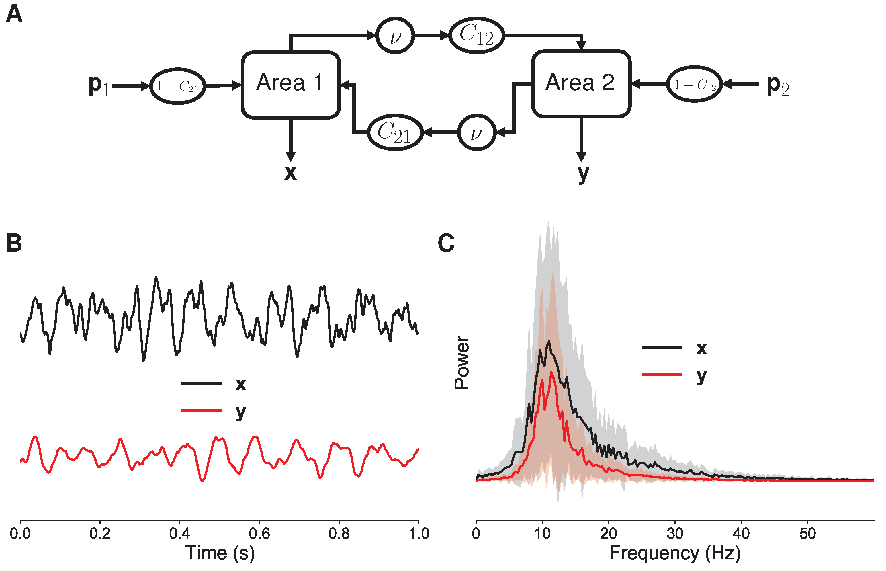
3.1. Neural Mass Models

Neural mass models (NMM) are biologically plausible mathematical descriptions of neural mechanisms [39]. They represent the electrical activity of neural populations at a macroscopic level through a set of stochastic differential equations [40]. NMMs allow generating mildly nonlinear time series with properties that resemble the oscillatory dynamics of electrophysiological signals, such as EEG, and how they change as a result of coupling between different cortical areas. Therefore, NMMs are useful to study the behavior of brain connectivity measures that aim to capture such interactions [8,24,40,41]. Figure 1A shows a schematic representation of an NMM with two interacting cortical areas from which two signals, $\mathbf{x}$ and $\mathbf{y}$ (see Figure 1B), can be obtained. The parameters $C_{12}$ and $C_{21}$ are known as coupling coefficients, and they determine the strength of the coupling from Area 1 to Area 2, and from Area 2 to Area 1, respectively. The parameter $\nu$ represents the interaction lag between the two areas, while ${\mathbf{p}}_1$ and ${\mathbf{p}}_2$ are external inputs coming from other cortical regions.

In this work, we use NMMs to generate interacting time series with known oscillatory properties in order to test the performance of the proposed phase TE estimator. In particular, we test our proposal in terms of its ability to detect directed interactions for different levels of coupling strength, under the presence of noise and signal mixing, and for bidirectional narrowband couplings. We proceed as follows: first, we set the model parameters describing Areas 1 and 2 as in [40], so as to generate signals with power spectrums peaking in the $\alpha$ (8 Hz–12 Hz) and lower $\beta$ bands (12–20 Hz), as depicted in Figure 1C. Then, in order to generate unidirectionally coupled signals, with interactions from $\mathbf{x}$ to $\mathbf{y}$, we set the parameter $C_{21}$ to 0 for all simulations. Also, the parameter $\nu$ is set to 20 ms, and the extrinsic inputs ${\mathbf{p}}_1$ and ${\mathbf{p}}_2$ are modeled as Gaussian noise [40]. Afterward, we generate 50 pairs (trials) of 3 s long signals, using a simulation time step of 1 ms, equivalent to a sampling frequency of 1000 Hz, for each condition in the three scenarios detailed in Section 3.1.1, Section 3.1.2 and Section 3.1.3. Next, we select a 2 s long segment from the signals, from 0.5 s to 2.5 s, and downsample them to 250 Hz. Then, we compute connectivity estimates for the simulated data in the frequency range between 2 Hz and 60 Hz, in steps of 2 Hz. After that, we obtain net connectivity values, defined as

$$\Delta \lambda (\mathbf{x},\mathbf{y},f)=\lambda (\mathbf{x}\to \mathbf{y},f)-\lambda (\mathbf{y}\to \mathbf{x},f),$$

(20)

where $\lambda$ stands for any of the phase-based effective connectivity measures studied, except for the PSI, in which case all subsequent analyses are performed directly on the PSI values. Lastly, for each condition in the three scenarios and at each frequency evaluated, we perform permutation tests based on randomized surrogate trials [34,42] to determine which net couplings or directed connections are statistically significant. The permutation test employed uses the trial structure of the data to generate surrogate datasets for the null hypothesis (absence of directed interactions). It does so by shuffling the data from different trials. The significance level for the tests was set to $3.3\times {10}^{-4}$ after applying the Bonferroni correction to an initial alpha level of $0.01$ in order to account for 30 independent tests, one for each evaluated frequency per condition.

3.1.1. Coupling Strength

In order to test the ability of our phase TE estimation method to detect phase-based directed interactions of varying intensity, we modify the coupling strength between the simulated signals, $\mathbf{x}$ and $\mathbf{y}$, by varying the parameter $C_{12}$ in the range $\{0,0.2,0.5,0.8\}$, with 0 indicating the absence of coupling and $0.8$ a strong interaction between the two signals.

3.1.2. Noise and Signal Mixing

To asses the robustness of our proposal to realistic levels of noise and signal mixing, we do the following: we generate a noise time series $\mathbf{\eta }$, with the same power spectrum of $\mathbf{x}$, through the methodology proposed in [8]. Then, we add $\mathbf{x}$ and $\mathbf{\eta }$ to generate a noisy version of $\mathbf{x}$, ${\mathbf{x}}_{\mathbf{\eta }}=\mathbf{x}+{10}^{-\frac{\mathrm{SNR}}{20}}\mathbf{\eta }$, where SNR is the signal to noise ratio. Likewise for $\mathbf{y}$. Then, we mix ${\mathbf{x}}_{\mathbf{\eta }}$ and ${\mathbf{y}}_{\mathbf{\eta }}$ to simulate one of the effects of volume conduction, by doing ${\mathbf{x}}_{\mathbf{\eta }}^w=\left(1-\frac{w}{2}\right){\mathbf{x}}_{\mathbf{\eta }}+\left(\frac{w}{2}\right){\mathbf{y}}_{\mathbf{\eta }}$, and ${\mathbf{y}}_{\mathbf{\eta }}^w=\left(1-\frac{w}{2}\right){\mathbf{y}}_{\mathbf{\eta }}+\left(\frac{w}{2}\right){\mathbf{x}}_{\mathbf{\eta }}$, with w the mixing strength. We set the parameters SNR and w to 3 and $0.25$ respectively, based on the results obtained in [8] for realistic values of noise and mixing for EEG signals. The coupling coefficient $C_{12}$ is held constant at a value of $0.5$ to simulate couplings of medium strength.

3.1.3. Narrowband Bidirectional Interactions

In this experiment, we aim to evaluate how our proposal deals with bidirectional interactions of localized frequency content. Particularly, we want to assess its performance for signals $\mathbf{x}$ and $\mathbf{y}$ containing a directed interaction from $\mathbf{x}$ to $\mathbf{y}$ at 10 Hz and an interaction in the opposite direction, from $\mathbf{y}$ to $\mathbf{x}$, at 40 Hz. To generate such signals, first, we modify the model parameters of Area 2 so that it produces a signal $\mathbf{y}$ with a power spectrum peaking in the $\gamma$ band [39]. The power spectrum of $\mathbf{x}$ remains as before. The coupling coefficient $C_{12}$ is again held constant at a value of $0.5$. The change in the parameters of Area 2 leads to strong directed interactions from $\mathbf{x}$ to $\mathbf{y}$ around 10 Hz and 40 Hz. Then, we use a Morlet wavelet (Equation (10)) to filter both $\mathbf{x}$ and $\mathbf{y}$ at those frequencies (10 Hz and 40 Hz). The obtained real-valued narrowband time series are then combined as follows: ${\mathbf{x}}_{*}={\mathbf{x}}_{10\mathrm{Hz}}+{\mathbf{y}}_{40\mathrm{Hz}}$ and ${\mathbf{y}}_{*}={\mathbf{y}}_{10\mathrm{Hz}}+{\mathbf{x}}_{40\mathrm{Hz}}$. Next, ${\mathbf{x}}_{*}$ and ${\mathbf{y}}_{*}$ are added to broadband noise generated following the same approach described in Section 3.1.2, with an SNR of 6.

3.2. EEG Data

In order to test the performance of our phase TE estimator in the context of BCI, we obtain effective connectivity features from EEG signals recorded under two different cognitive paradigms: the first one consisting of motor imagery (MI) tasks and the second one of a change detection task designed to study working memory (WM). Our aims are to set up classification systems that allow discriminating between the conditions in each paradigm, using as inputs relevant directed interactions among EEG signals and then evaluate their performance in relation to the connectivity measures used to train them. To those ends, we employ two publicly available databases: the BCI Competition IV database 2a (http://www.bbci.de/competition/iv/index.html, accessed on 2 June 2021) and a database from brain activity during visual working memory (https://data.mendeley.com/datasets/j2v7btchdy/2, accessed on 2 June 2021).

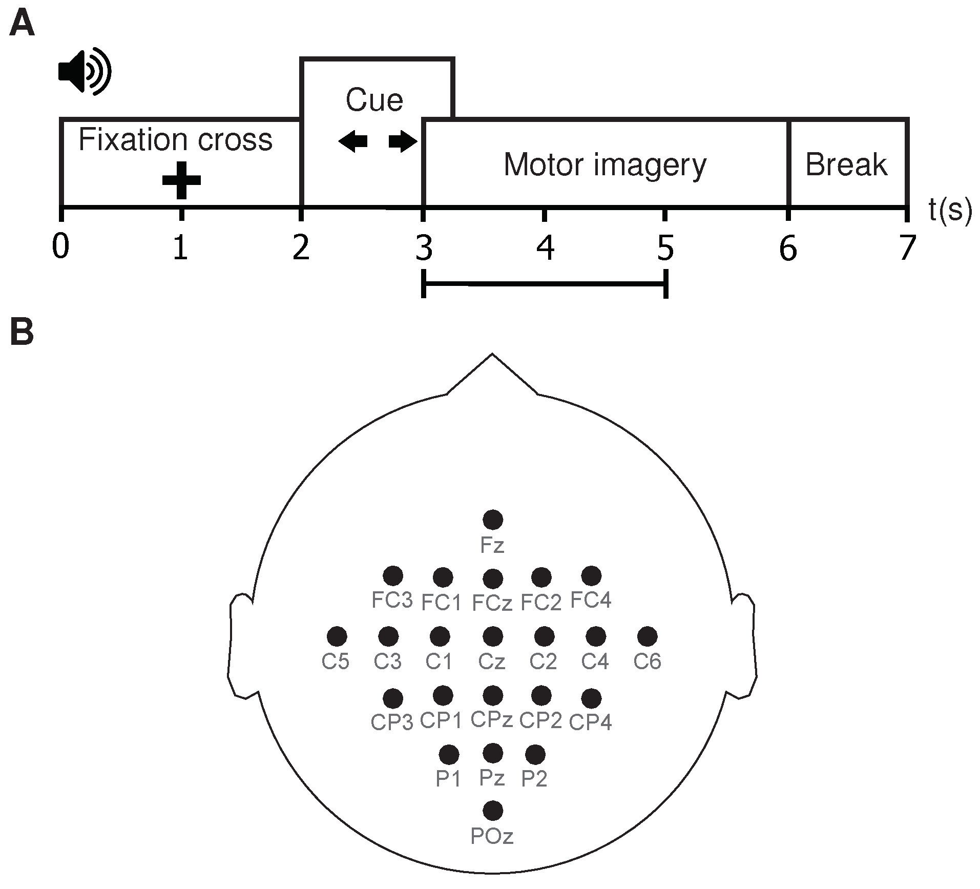
3.2.1. Motor Imagery

Motor imagery (MI) is the process of mentally rehearsing a motor action, such as moving a limb, without actually executing it [43]. The BCI Competition IV database 2a [44] comprises EEG data from 9 healthy subjects recorded during an MI paradigm consisting of four different MI tasks, namely, imagining the movement of the left hand, the right hand, both feet, or the tongue. Each trial of the paradigm starts with a fixation cross displayed on a computer screen, along with a beep. At second 2, a visual cue appears on the screen for a period of 1.25 s (an arrow pointing left, right, down, or up, corresponding to one of the four MI tasks). The cue prompts the subject to perform the indicated MI task until the cross vanishes from the screen at second 6. A representation of the paradigm’s time course is shown in Figure 2A. Each subject performed 144 trials per MI task. The EEG data are acquired at a sampling rate of 250 Hz, from 22 Ag/AgCl electrodes ($C=22$) placed according to the international 10/20 system, as depicted in Figure 2B. Next, the data are bandpass-filtered between 0.5 Hz and 100 Hz. A 50 Hz Notch filter is also applied. For each subject, the database contains a training dataset and a testing dataset, obtained following the same experimental paradigm [44]. In this study, we consider a bi-class classification problem involving the left and right hand MI tasks, so we drop the trials associated with the feet and the tongue. Afterward, we also drop the trials marked for rejection in the database itself [44]. Then, for all trials we select a 2 s long time window stretching from second 3 to second 5 ($M=500$ samples), as schematized in Figure 2A. Finally, we compute the surface Laplacian of each remaining trial through the spherical spline method for source current density estimation, in order to reduce the deleterious effects of volume conduction on connectivity analyses [21,45,46].

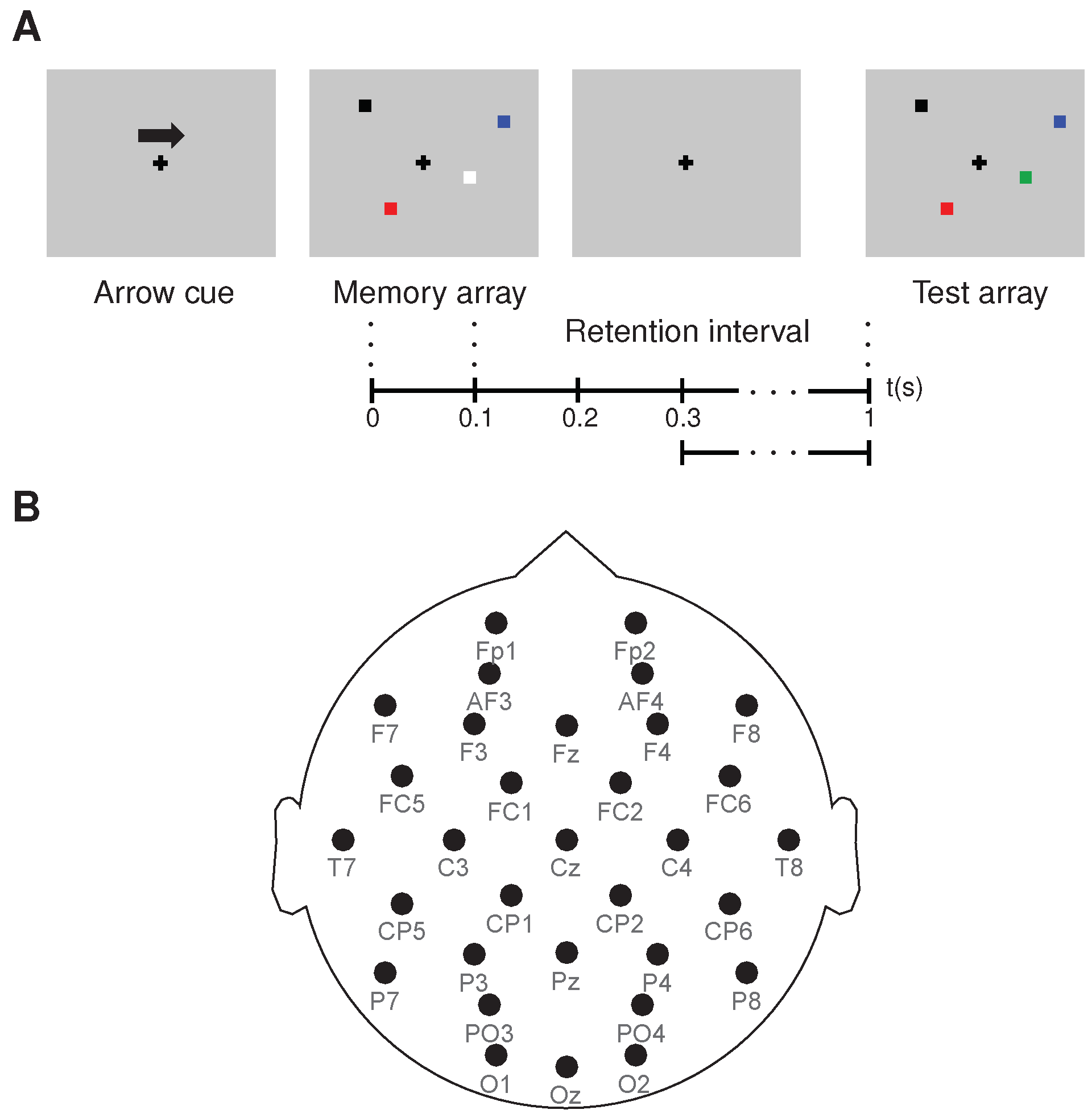
3.2.2. Working Memory

The concept of working memory (WM) refers to a cognitive system of limited capacity that allows for temporary storage and manipulation of information [47]. The database from brain activity during visual working memory, presented in [48], contains EEG data recorded from twenty-three subjects, with normal or corrected-to-normal vision, and without color-vision deficiency, while performing multiple trials of a change detection task [49]. The task consists of remembering the colors of a set of squares, termed memory array, and then comparing them with the colors of a second set of squares located in the same positions, termed test array. A trial of the task begins with an arrow indicating either the left or the right side of the screen. Then, a memory array appears on the screen for 0.1 s. For every trial, memory arrays are displayed on both hemifields, but the subject must remember only those appearing on the side indicated by the arrow cue. Next, after a retention period lasting 0.9 s, a test array appears. The subject then reports if the colors of all the items in the memory and test arrays match. The task has three levels according to the number of elements in the memory array: low memory load (one square), medium memory load (two squares), and high memory load (four squares). A representation of the above-described experimental paradigm is depicted in Figure 3A. The color of one of the squares in the test array differs from its counterpart in the memory array in 50% of the trials. Each subject performed a total of 96 trials, with 32 trials for each memory load level. The EEG data are acquired at a sampling rate of 2048 Hz, using 64 electrodes (Biosemi ActiveTwo) arranged according to the international 10/20 extended system, as depicted in Figure 2B. Besides the EEG data, the database provides recordings from four EOG channels and two externals electrodes located on the left and right mastoids.

In this study, we perform the following preprocessing steps before any further data analysis. First, we re-reference the data to the average of the mastoid channels. Next, we bandpass-filter the data between 0.01 Hz and 20 Hz using a Butterworth filter of order 2. Afterward, we extract the trial information from the continuous EEG data using a 1.4 s squared window. Each trial segment starts 0.2 s before the presentation of the memory array. Then, we perform a visual inspection of the data and discard two subjects (subjects number 11 and 17) because of the presence of strong artifacts in a very large number of trials. Subjects number 22 and 23 are reassigned as subjects 17 and 11, respectively. After that, we remove ocular artifacts from the EEG data by performing independent component analysis (ICA) on it and then eliminating the components that more closely resemble the information provided by the EOG data [48]. Then, we discard all incorrect trials, i.e., trials for which the subjects incorrectly matched the memory and test arrays. Next, we select 32 out of the 64 channels in the EEG data ($C=32$), as shown in Figure 3B. Then, we downsample the data to 1024 Hz, and segment, for each trial, the time window starting 0.3 s after the onset of the memory array and ending just before the presentation of the test array (see Figure 3A). The 0.7 s long segments ($M=717$) cover most of the retention interval, the period when the subjects should maintain the stimulus information in their working memories, while leaving out any purely sensory responses elicited immediately after the presentation of the stimulus. Finally, with the aim of reducing the presence of spurious connections associated with volume conduction effects, we compute the surface Laplacian of each trial.

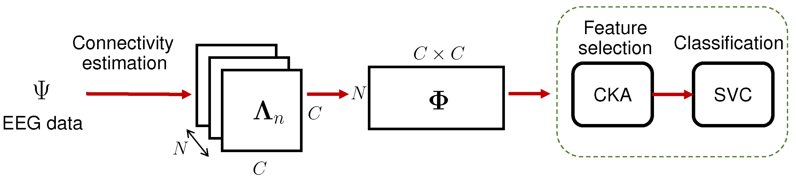
3.2.3. Classification Setup

Feature Extraction

Let $\Psi ={\{{\mathbf{X}}_n\in {\mathbb{R}}^{C\times M}\}}_{n=1}^N$ be an EEG set holding N trials from either an MI or a WM dataset, recorded from a single subject, where C stands for the number of channels and M corresponds to the number of samples. In addition, let ${\left\{l_n\right\}}_{n=1}^N$ be a set whose n-th element is the label associated with trial ${\mathbf{X}}_n$. For the MI database $l_n$ can take the values of 1 and 2, corresponding to right hand and left hand motor imagination, respectively. Similarly, for the WM database, $l_n$ can take the values of 1, 2, and 3 corresponding to low, medium, and high memory loads. In both cases, our goal is to estimate the class label from relevant effective connectivity features extracted from ${\mathbf{X}}_n$. Because of the results obtained for the simulated data (see Section 4.1 for details), here we consider features from only three approaches for phase-based effective connectivity estimation, namely, TE${}_{\kappa \alpha }^{\theta }$, GC${}^{\theta }$, and PSI. Additionally, we also characterize the data through the real-valued versions of TE${}_{\kappa \alpha }$ and GC.

For the real-valued effective connectivity measures considered, we do the following: let $\lambda ({\mathbf{x}}_c\to {\mathbf{x}}_{c^{\prime }})$ be a measure of effective connectivity between channels ${\mathbf{x}}_c,{\mathbf{x}}_{c^{\prime }}\in {\mathbb{R}}^M$. By computing $\lambda ({\mathbf{x}}_c\to {\mathbf{x}}_{c^{\prime }})$ for each pairwise combination of channels in ${\mathbf{X}}_n$ we obtain a connectivity matrix $\mathsf{\Lambda }\in {\mathbb{R}}^{C\times C}$. In the case when $c=c^{\prime }$, we set $\lambda ({\mathbf{x}}_c\to {\mathbf{x}}_{c^{\prime }})=0$. Then, we normalize $\mathsf{\Lambda }$ to the range $[0,1]$. After performing the above procedure for the N trials, we get set of connectivity matrices ${\{{\mathsf{\Lambda }}_n\in {\mathbb{R}}^{C\times C}\}}_{n=1}^N$. Then, we apply vector concatenation to ${\mathbf{\Lambda }}_n$ to yield a vector ${\mathit{\varphi }}_n\in {\mathbb{R}}^{1\times (C\times C)}$. Next, we stack the N vectors ${\mathit{\varphi }}_n$, corresponding to each trial, to obtain a matrix $\mathsf{\Phi }\in {\mathbb{R}}^{N\times (C\times C)}$ holding all directed interactions, estimated through $\lambda$, for the EEG set $\mathsf{\Psi }$. A graphical representation of the above-described steps, as well as of our overall classification setup, is depicted in Figure 4.

For the phase-based effective connectivity measures of interest, we proceed in a similar fashion: let ${\lambda }^{\theta }({\mathbf{x}}_c\to {\mathbf{x}}_{c^{\prime }},f)$ be a measure of phase-based effective connectivity between channels ${\mathbf{x}}_c,{\mathbf{x}}_{c^{\prime }}$ at frequency f. By computing ${\lambda }^{\theta }({\mathbf{x}}_c\to {\mathbf{x}}_{c^{\prime }},f)$ for each pairwise combination of channels in ${\mathbf{X}}_n$ we obtain a connectivity matrix $\mathsf{\Lambda }(f)\in {\mathbb{R}}^{C\times C}$ (when $c=c^{\prime }$, we set ${\lambda }^{\theta }({\mathbf{x}}_c\to {\mathbf{x}}_{c^{\prime }},f)=0$). For the MI database, we vary the values of f in the range from 8 Hz to 18 Hz, in 2 Hz steps, since activity in that frequency range has been associated with MI tasks [43]. Then we define two bandwidths of interest $\Delta f\in \{\alpha \in [8-12],{\beta }_l\in [14-18]\}$ Hz. Afterward, we average the matrices $\mathsf{\Lambda }(f)$ within each bandwidth, normalize the resulting matrices to the range $[0,1]$, and stack them together, so that for each trial we have a connectivity matrix ${\mathsf{\Lambda }}^{\prime }\in {\mathbb{R}}^{C\times C\times 2}$. Therefore, for the N trials, we get set of connectivity matrices ${\{{\mathsf{\Lambda }}_n^{\prime }\in {\mathbb{R}}^{C\times C\times 2}\}}_{n=1}^N$. Then, we apply vector concatenation to ${\mathsf{\Lambda }}_n^{\prime }$ to yield a vector ${\mathit{\varphi }}_n\in {\mathbb{R}}^{1\times (C\times C\times 2)}$. After that, we stack the N vectors ${\mathit{\varphi }}_n$ in order to obtain a single matrix $\mathsf{\Phi }\in {\mathbb{R}}^{N\times (C\times C\times 2)}$ characterizing $\mathsf{\Psi }$ for the MI data. For the WM we follow the same steps, only that in this case we vary the values of f in the range from 4 Hz to 18 Hz, in 2 Hz steps, since oscillatory activity at those frequencies has been shown to play a role in the interactions between different brain regions during WM [50,51]. Next, we define three bandwidths of interest $\Delta f\in \{\theta \in [4-6],\alpha \in [8-12],{\beta }_l\in [14-18]\}$ Hz, which leads to a connectivity matrix ${\mathsf{\Lambda }}^{\prime }\in {\mathbb{R}}^{C\times C\times 3}$ for each trial and ultimately to a matrix $\mathsf{\Phi }\in {\mathbb{R}}^{N\times (C\times C\times 3)}$ characterizing $\mathsf{\Psi }$ for the WM data. Note that since the PSI is an antisymmetric connectivity measure, we only use the upper triangular part of the connectivity matrix associated with each trial to build $\mathsf{\Phi }$.

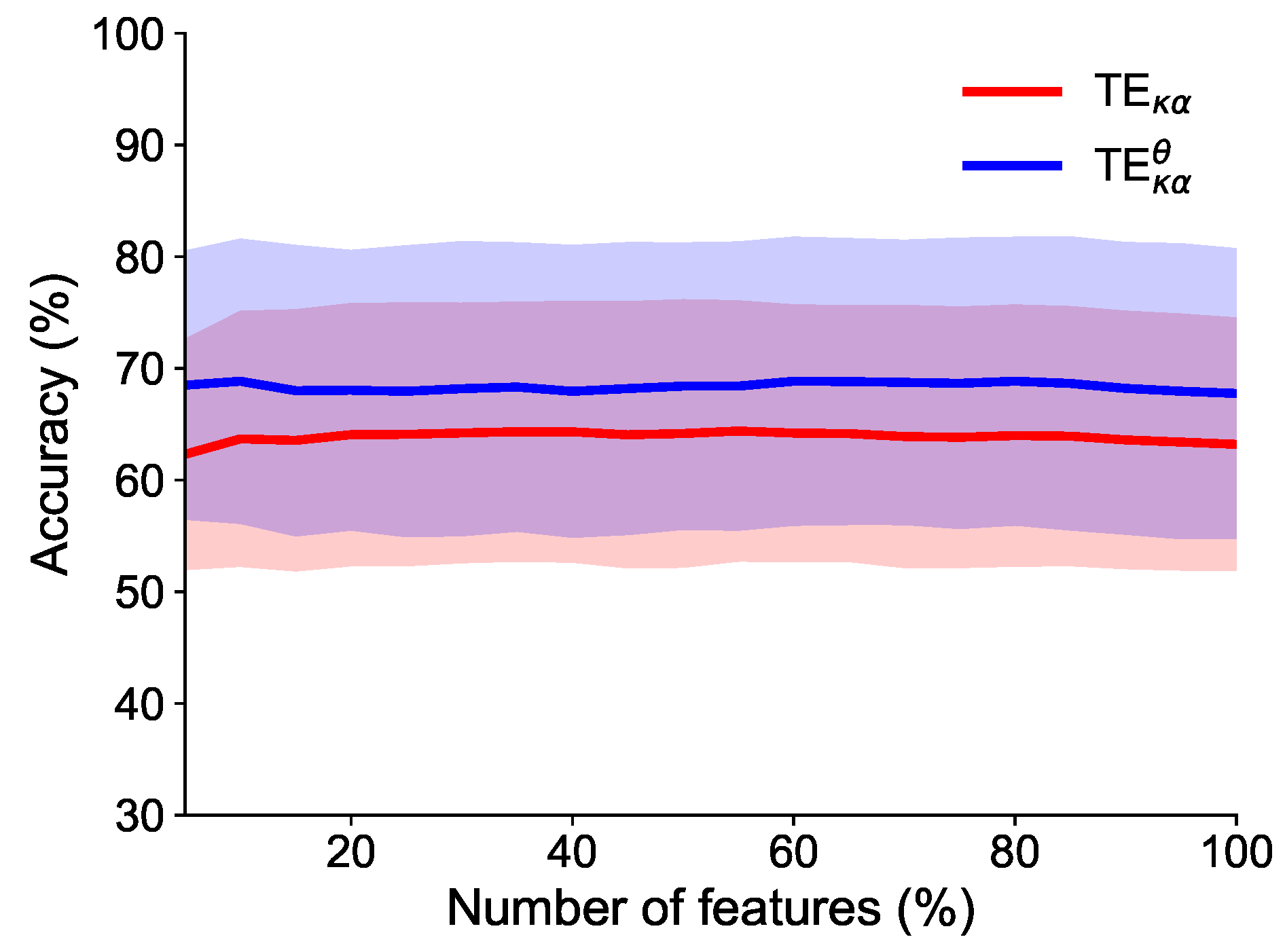
Feature Selection and Classification

After characterizing the EEG data, either through real-valued or phase-based effective connectivity measures, we set up a subject-dependent classification system for the MI and WM databases.

For the MI data, we do the following: Since the MI database has training and testing datasets, we divide our classification system into a training-validation stage and a testing stage. For the training-validation stage, we first specify a cross-validation scheme of 10 iterations. For each iteration, 70% of the trials of the training dataset are randomly assigned to a training set and the remaining 30% to a validation set. Then, we use CKA (see Section 2.4) over the connectivity features obtained from the training set to generate a relevance vector $\mathbf{\varrho }\in {[0,1]}^P$, where P equals the number of features in $\mathsf{\Phi }$. P varies according to the connectivity measure used to characterize the data. Then, we use $\mathbf{\varrho }$ to rank $\mathsf{\Phi }$. Next, we select a varying percentage of the ranked features, from 5% to 100% in 5% steps, and input them to the classification algorithm. The features associated with the highest values of $\mathbf{\varrho }$ are input first, and as the percentage of features increases those associated with lower values of $\mathbf{\varrho }$ are progressively included. In this work, we use a support vector classifier (SVC) with an RBF kernel [52]. All classification parameters, including the percentage of discriminant features, are tuned at this stage through a grid search. We select the parameters according to the classification accuracy, aiming to improve the system’s performance. Then, for the testing stage, we train an SVC using the connectivity features from all trials in the training dataset as well as the parameters found in the previous stage. Lastly, we quantify the performance of the trained system in terms of the classification accuracy, obtained after predicting the MI task class labels of the testing dataset from its connectivity features.

The classification system we set up for the WM data closely resembles the one previously detailed for the MI data, with three changes. First, the WM database consists of one set of data for each subject, instead of two, so there is only a training-validation stage. Second, given the reduced number of trials available for each memory load level, each of the 10 iterations of the cross-validation scheme follows an 80–20% split for the training and validation sets (instead of a 70–30% split). Third, since the results provided by CKA are not stable for the low number of trials available from each subject (27.7 trials per class, on average), we opted to add an auxiliary cross-validation step, with the same characteristics as the one described above, and use it to estimate a single relevance vector $\overline{\mathbf{\varrho }}$, obtained as the average of the relevance vectors of each data split. Then, we use $\overline{\mathbf{\varrho }}$ to perform feature selection in every iteration of the main cross-validation scheme.

3.3. Parameter Selection

We used in-house Python implementations of the algorithms for all the connectivity measures studied (The TE${}_{\kappa \alpha }^{\theta }$ implementation is available at https://github.com/ide2704/Kernel_Phase_Transfer_Entropy, accessed on 13 July 2021), except for TE${}_{KSG}^{\theta }$. In that case, we used the implementation provided by the open access toolbox TRENTOOL, a TE estimation and analysis toolbox for Matlab [34].

Regarding the selection of parameters involved in the different effective connectivity estimation methods, we proceeded as follows: For the TE methods, we estimated all parameters from the real-valued time series, i.e., before extracting the phase time series. The embedding delay $\tau$ was set to 1 autocorrelation time (ACT), as proposed in [31]. The embedding dimension d was selected from the range $d=\{1,2,\dots ,10\}$ using Cao’s criterion [34,53]. Note that for any signal pair, the embedding parameters selected are those of the driven or target time series, i.e., to estimate TE$(\mathbf{x}\to \mathbf{y})$ we use for both time series the embedding parameters found for $\mathbf{y}$. The interaction delay u was set as the value generating the largest TE from ranges that varied depending on the experiment: $u=\{1,2,\dots ,10\}$ for the NMMs, $u=\{1,4,\dots ,25\}$ for the MI data, and $u=\{50,60,\dots ,250\}$ for the WM data. Note that the meaning of u in terms of the time delay of the directed interaction between the driving and driven systems is associated with the sampling frequency, e.g., $u=\{1,2,\dots ,10\}$ for data sampled at 250 Hz translates to a time range between 4 ms and 40 ms. For TE${}_{\kappa \alpha }^{\theta }$ we select a value of $\alpha =2$, which is neutral to weighting, a convenient choice when there is no previous knowledge about the values of the $\alpha$ parameter better suited for a particular application [10,28]. In addition, as kernel function, we employ an RBF kernel with Euclidean distance (see Equation (13)). The bandwidth $\sigma$ was set in each case as the median distance of the data [54]. For TE${}_{KSG}^{\theta }$ the Theiler correction window and the number of neighbors were left at their default values in TRENTOOL, 4 and 1 ACT, respectively [34]. For the GC methods the order of the autoregressive models o was selected from the range $o=\{1,3,\dots ,9\}$ using Akaike information criterion [55,56]. Furthermore, in order to estimate the PSI we employed a sliding window 5 frequency bins long (3 bins long for the WM data), centered on the frequency of interest. Finally, for all the connectivity methods involving the extraction of phase time series through Morlet wavelets, we varied the parameter m (see Equation (10)) from 3 to 10 in a logarithmic scale, according to the selected frequency of the filter.

4. Results and Discussion

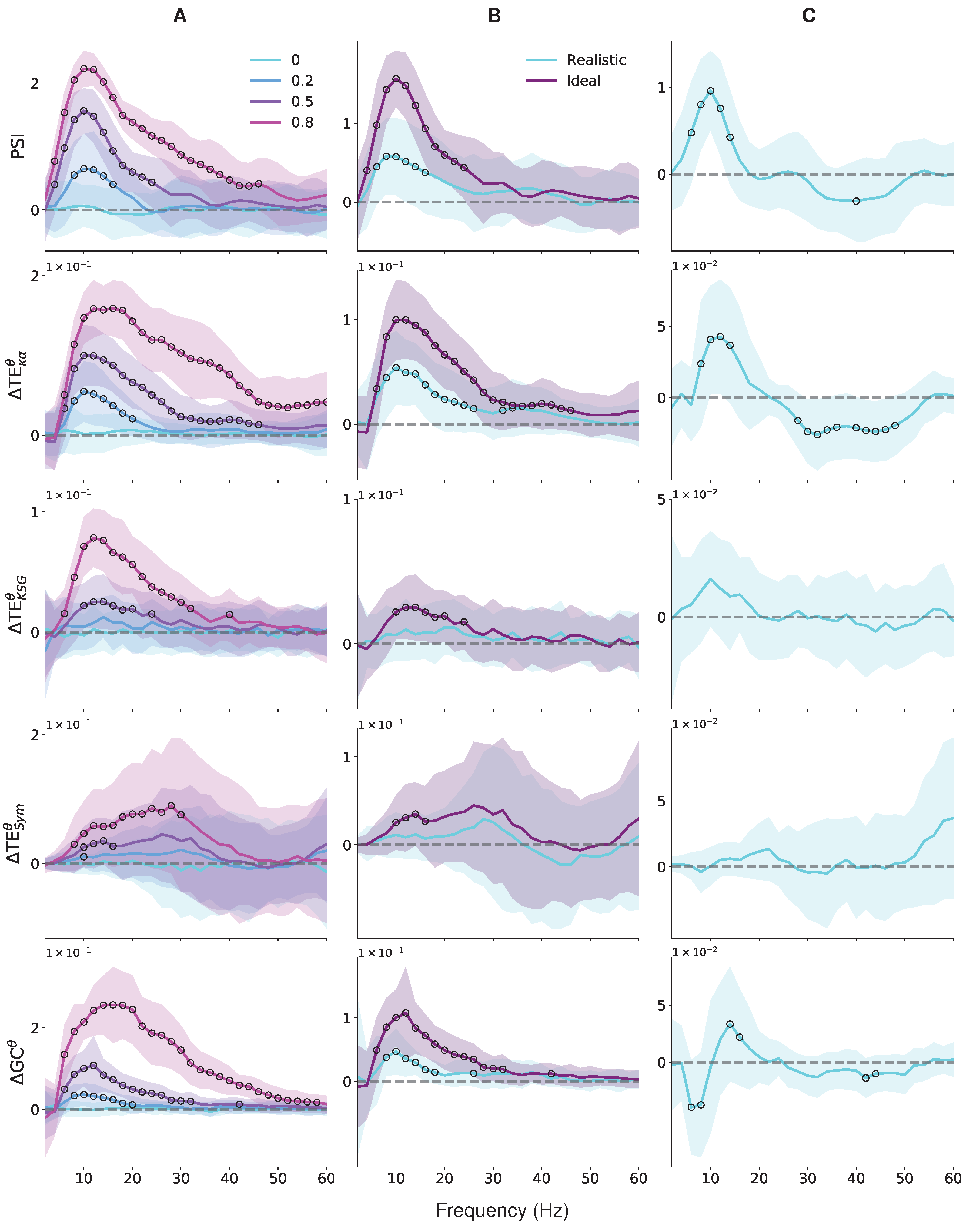
4.1. Neural Mass Models Results

The experiments described in Section 3.1 are intended to assess whether the phase-based connectivity measures considered in this study correctly detect the direction of interaction between two time series of known oscillatory properties. Figure 5 presents the results obtained from such experiments. Namely, column A shows the connectivity values obtained for different levels of coupling strength, column B compares the connectivities estimated for ideal signals with those of signals contaminated with noise and mixing, and column C displays the results obtained for bidirectional narrowband couplings. The rows in Figure 5 correspond to each of the phase-based connectivity measures studied. The first row contains average PSI values computed on the frequency range between 2 Hz and 60 Hz, while rows two to five display average net connectivity values for TE${}_{\kappa \alpha }^{\theta }$, TE${}_{KSG}^{\theta }$, TE${}_{Sym}^{\theta }$, and GC${}^{\theta }$, respectively. Circled values indicate statistically significant connectivities at a particular frequency, according to a permutation test based on randomized surrogate trials. The test identifies connectivity values that are, on average, significantly different from those expected for that connectivity measure applied to non-interacting signals. For the three experiments involving simulated data from NMMs, we use the PSI as a comparison standard, since it is a robust and well-stablished measure of linear directed interactions defined in terms of phase relations [12,13]. Therefore, it is suited to analyze the coupled, mildly nonlinear time series generated by NMMs.

Regarding the first experiment, which modifies the coupling strength between the simulated signals, the obtained results (Figure 5, column A) show that all the measures studied satisfactorily detect the coupling direction of the simulated data. Note that since we set the NMMs to generate unidirectional interactions from $\mathbf{x}$ to $\mathbf{y}$, and because of the way we defined $\Delta \lambda$, then all net connectivity values for the simulated coupled signals should be positive. The same is true for the PSI$(\mathbf{x}\to \mathbf{y})$. On the other hand, only the PSI, TE${}_{\kappa \alpha }^{\theta }$, and GC${}^{\theta }$ fulfill the criteria for an overall description of the phase-based interactions present in the data. First, we observe higher net connectivity values at higher coupling strengths, that is to say, stronger interactions lead to larger connectivity estimates. Second, for each coupling strength, there are higher net connectivity values around the frequencies corresponding to the main oscillatory components of the time series generated by the NMMs, in this case, oscillations in the range between 8 Hz and 20 Hz. Thirdly, there are statistically significant results for all the coupling strengths explored, except for non-interacting time series ($C_{12}=0$). TE${}_{KSG}^{\theta }$ does not capture statistically significant interactions for a coupling coefficient value of 0.2, indicating a lower sensitivity to weak couplings. While TE${}_{Sym}^{\theta }$ exhibits a very distorted connectivity profile when compared with the PSI. In addition, it has much larger standard deviations for all the coupling strengths considered.

The second experiment assesses the robustness of our proposal to realistic levels of noise and signal mixing, two sources of signal degradation that can lead to spurious connectivity results. In electrophysiological signals, such as EEG, signal mixing arises as a result of field spread, while noise is the result of technical and physiological artifacts [9,57,58]. The results in Figure 5, column B, show that PSI, TE${}_{\kappa \alpha }^{\theta }$, and GC${}^{\theta }$ capture statistically significant interactions in the frequencies of interest for both the ideal (no noise or signal mixing) and realistic conditions. The smaller connectivity values for the data contaminated with noise and signal mixing, as compared with the ideal signals, are mostly explained by the reduction in asymmetry between the driving and driven signals caused by mixing [8]. On the contrary, we observe that neither TE${}_{Sym}^{\theta }$ nor TE${}_{KSG}^{\theta }$ produce statistically significant results under the realistic scenario, indicating that those estimators are less robust to signal degradation.

Finally, the third experiment aims to evaluate how our proposal deals with bidirectional interactions of localized frequency content. Because of our experimental setup, the obtained results should exhibit a positive deflection around 10 Hz in order to capture the directed interaction from $\mathbf{x}$ to $\mathbf{y}$ and a negative deflection around 40 Hz to represent the directed interaction from $\mathbf{y}$ to $\mathbf{x}$. Figure 5, column C, shows that both PSI and TE${}_{\kappa \alpha }^{\theta }$ successfully detect the change in the direction of interaction in localized frequency bands, with statistically significant connectivity values around the frequencies of interest. However, under this scenario, TE${}_{\kappa \alpha }^{\theta }$ is less frequency specific for high-frequency interactions than PSI, with statistically significant connections present for a large range of frequency values around 40 Hz. This is probably due to the filtering step involved in the estimation of TE${}_{\kappa \alpha }^{\theta }$, while PSI is directly defined on the data spectra. Additionally, TE${}_{KSG}^{\theta }$ and TE${}_{Sym}^{\theta }$ fail to produce any significant results, while GC${}^{\theta }$ shows a statistically significant, non-existing coupling from $\mathbf{y}$ to $\mathbf{x}$ for frequencies under 10 Hz. Note that, ultimately, the permutation test indicates whether the connectivity values obtained are unlikely to be the result of chance and not whether they correctly capture the directed interactions present in the data. In this case, the statistically significant results mean that GC${}^{\theta }$ consistently found a directed interaction from $\mathbf{y}$ to $\mathbf{x}$ in the range mentioned before.

The results discussed above indicate that the proposed phase TE estimator is able to detect directed interactions between time series resembling electrophysiological data for different levels of coupling strength, under the presence of noise and signal mixing and for bidirectional narrowband couplings. Furthermore, they show that it is competitive with well-established approaches for phase-based net connectivity estimation, such as PSI, in the case of weakly nonlinear signals. Lastly, our results also show that commonly used single-trial TE estimators, such TE${}_{KSG}$ and TE${}_{Sym}$, are ill-suited to measure directed interactions between instantaneous phase time series.

4.2. EEG Data Results

Table 1. MI and WM classification results in terms of the classification accuracy for all the effective connectivity measures considered.

	Motor Imagery (acc %)		Working Memory (acc %)
	Cross-Validation	Testing	Cross-Validation
GC [11]	$64.3\pm 11.7$	$57.1\pm 11.0$	$53.0\pm 7.4$
TE${}_{\mathbf{\kappa }\mathbf{\alpha }}$ [10]	$65.5\pm 11.4$	$62.8\pm 11.7$	$67.5\pm 4.2$
PSI [12,51]	$62.4\pm 7.8$	$58.8\pm 8.3$	$75.2\pm 5.2$
GC${}^{\mathbf{\theta }}$	$67.0\pm 11.9$	$63.5\pm 14.4$	$74.5\pm 4.4$
TE${}_{\mathbf{\kappa }\mathbf{\alpha }}^{\mathbf{\theta }}$	$\mathbf{70.4}\pm \mathbf{12.5}$	$\mathbf{69.0}\pm \mathbf{14.8}$	$\mathbf{93.0}\pm \mathbf{5.9}$

presents the average accuracies achieved by the proposed classification systems for both the MI and WM databases, for each effective connectivity method studied. For the MI database, in the training-validation stage, the classifier based on TE${}_{\kappa \alpha }^{\theta }$ features exhibited the highest average performance, closely followed by the one based on GC${}^{\theta }$. In the testing stage, we observe the same overall accuracy ranking, although a smaller drop in the classification accuracy occurs for TE${}_{\kappa \alpha }^{\theta }$ than for GC${}^{\theta }$, which points to a better generalization capacity by the system trained using features extracted through phase TE. For the WM database, the classifier trained from TE${}_{\kappa \alpha }^{\theta }$ features also displays the highest average accuracy. However, in this case, there is a large gap in performance between the TE${}_{\kappa \alpha }^{\theta }$-based classification system and the closest results from an alternative approach. Furthermore, the results in Table 1 show a consistent improvement in performance between the classifiers that use real-valued TE estimates and those that are trained from phase TE values. They also show relatively low accuracies for the classifiers trained using PSI features. We believe the latter can be explained by two factors. First, by definition, the PSI is unable to explicitly detect bidirectional interactions. It measures connectivity in terms of lead/lag relations, which leads to ambiguity regarding the meaning of PSI values close to zero, since they can be the result of either the lack of interaction or evenly balanced bidirectional connections. If the relevant information to discriminate among the conditions of a cognitive paradigm is related to the bidirectionality of interactions, such as those present in WM [50,51], then the PSI might not be an adequate characterization strategy. Secondly, the PSI, like GC, is a linear measure; its performance degrades for strongly nonlinear phase relationships.

In the sections below, we detail and further discuss the results obtained for each database.

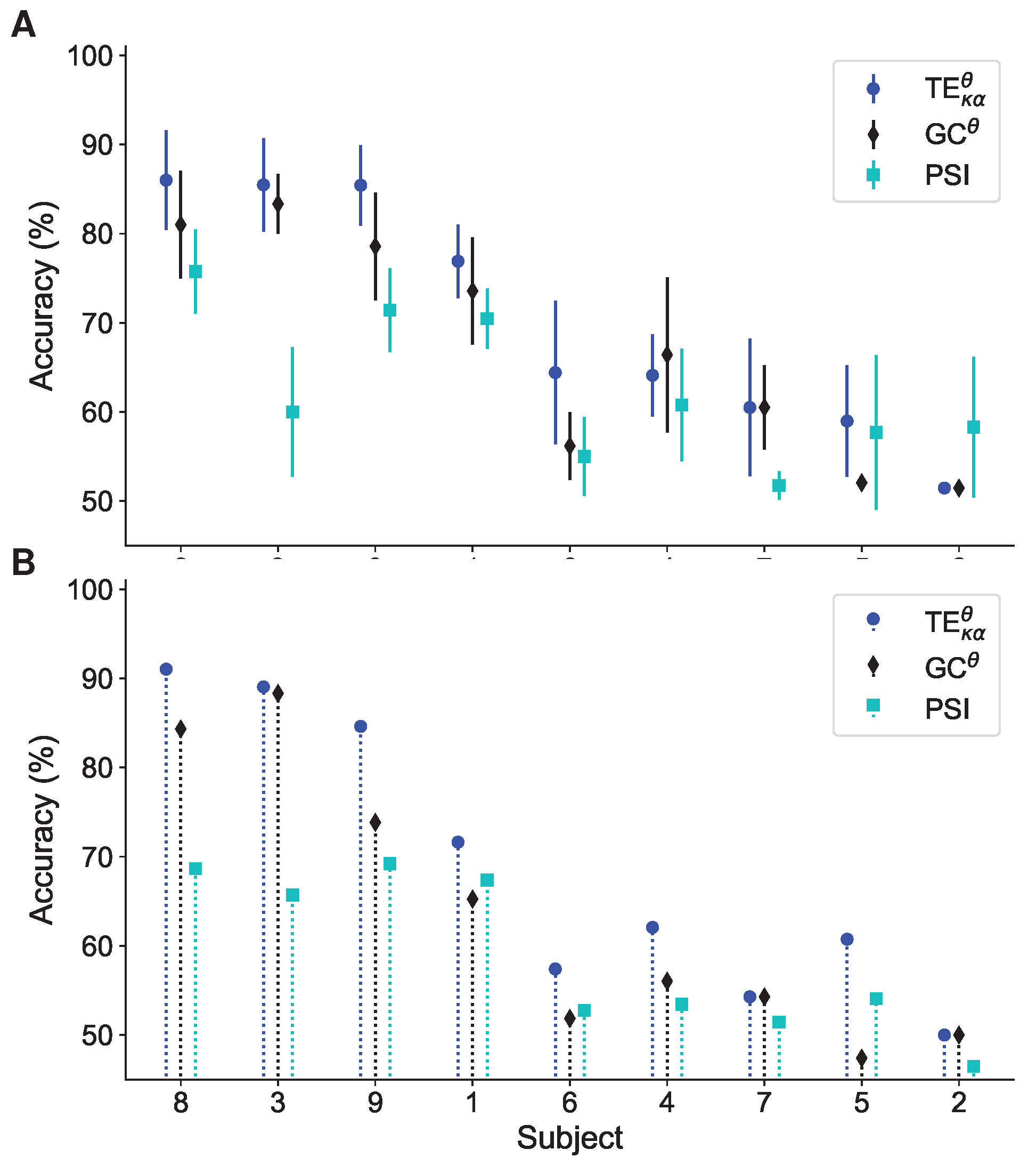
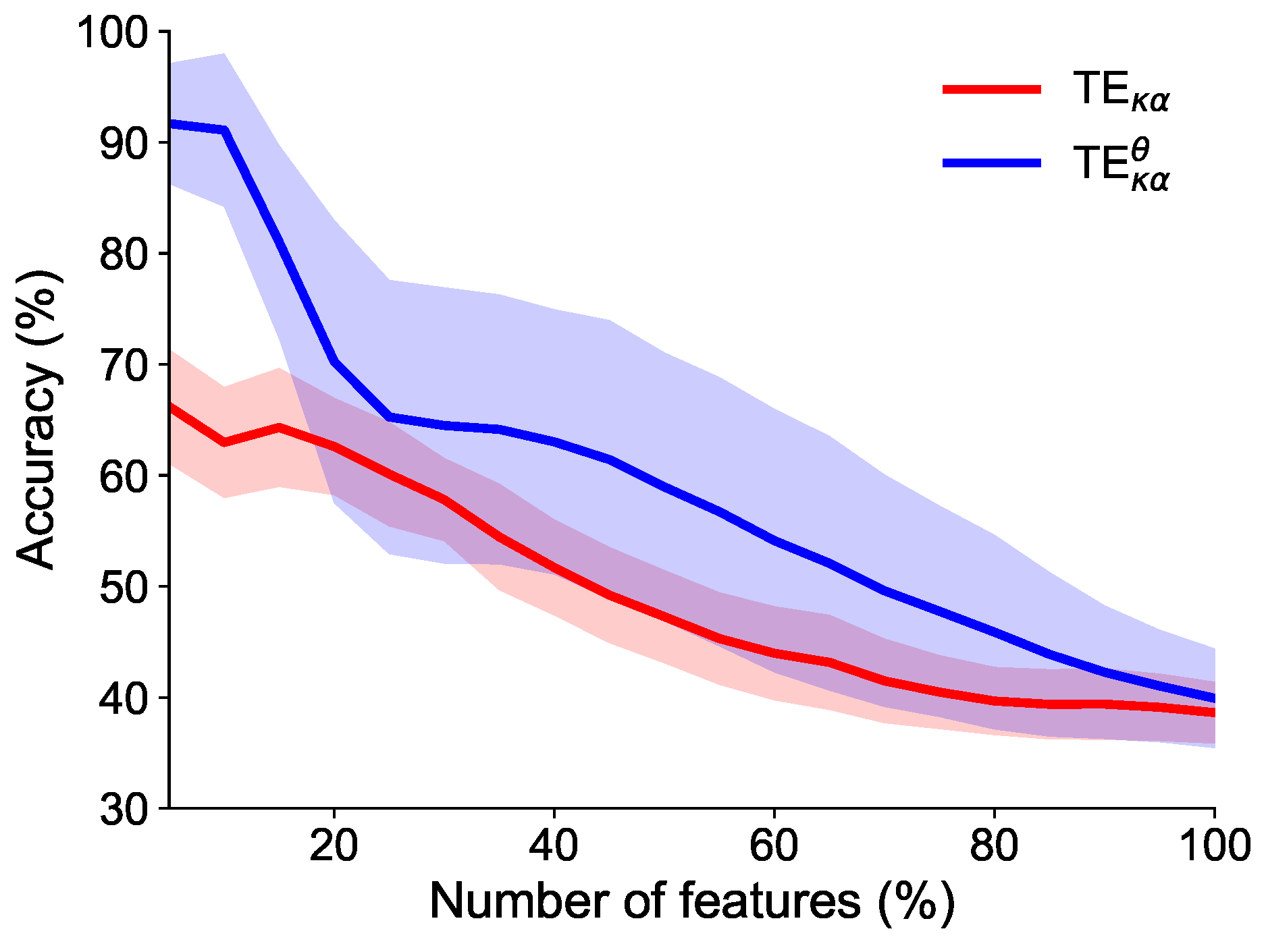
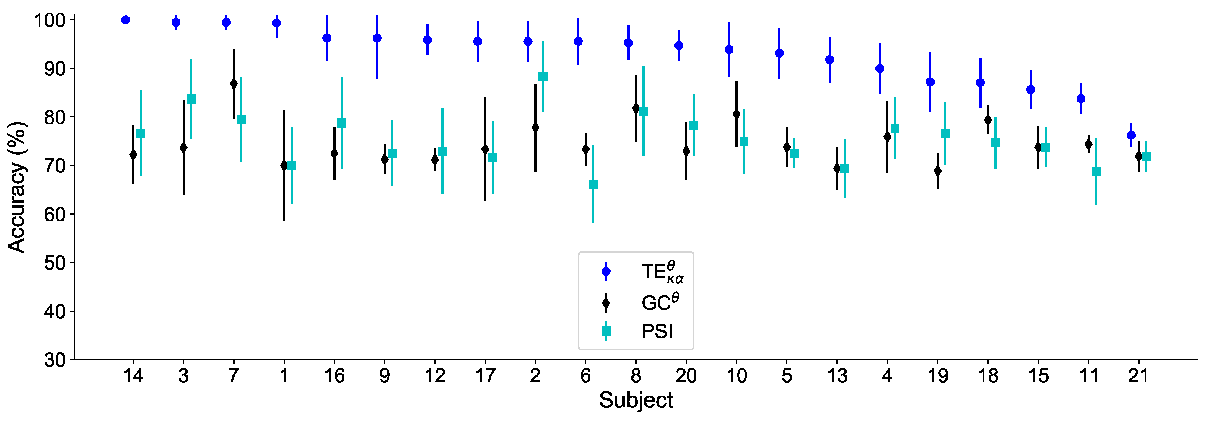
4.2.1. Motor Imagery Results

Figure 6 depicts the average classification accuracy for all subjects in MI database as a function of the number of selected features during the training-validation stage, for TE${}_{\kappa \alpha }$ and TE${}_{\kappa \alpha }^{\theta }$. These results show there is a small improvement in the ability to discriminate between the MI tasks when using features extracted through phase TE, as compared with real-valued TE. In addition, they reveal that the CKA-based feature selection strategy successfully identified the most relevant connections for MI task classification. That is to say, the classification system has a stable performance even for a very reduced number of connectivity features. This is fundamental for any practical BCI application that intends to use phase TE as a characterization strategy, since estimating single-trial phase TE is computationally expensive [8]. Therefore, it is important to reduce as much as possible the number of channel pair connectivity features required to achieve peak classification performance. Additionally, it is important to highlight that while classification accuracies in Figure 6, and in Table 1, are in the same range of those obtained through other connectivity-based characterization approaches [10,23], they are far below those obtained from methods such as common spatial patterns [59,60,61]. A possible explanation is that bivariate TE might be more robust at describing long-range interactions rather than local ones [41], like those arising from MI-related activity, centered on the sensorimotor area. In addition, the differences with the results in [10], where we used TE${}_{\kappa \alpha }$ to characterize the same database, lay mostly in the fact that in this study we select and analyze one 2 s long time window covering the period right after the end of the visual cue, while in [10] we report results from multiple overlapping windows covering the entirety of the task. Lastly, the large standard deviations from the average accuracies in Figure 6 point to disparate performances for different subjects.

Figure 7A shows the highest average classification accuracy per subject for TE${}_{\kappa \alpha }^{\theta }$, GC${}^{\theta }$ and PSI, during the training-validation stage. The subjects are ordered from highest to lowest performance. The analogous information for the testing stage is presented in Figure 7. In both stages, the TE${}_{\kappa \alpha }^{\theta }$-based classifier performs slightly better than those based on alternative connectivity estimation strategies in most subjects. In addition, as inferred from Figure 6, there are large variations in performance for the different subjects in the database, consistent across the two classification stages. This behavior has been reported elsewhere [10,59,60,61,62].

In order to gain insight into the observed performance differences, in the case of TE${}_{\kappa \alpha }^{\theta }$, we exploited the second advantage provided by the CKA-based relevance analysis. The relevance vector index $\mathbf{\varrho }$ not only allows us to perform feature selection but also provides a one-to-one relevance mapping to each connectivity feature. That is to say, we can reconstruct normalized relevance connectivity matrices by properly reshaping $\mathbf{\varrho }$, so as to visualize the connectivity pairs and frequency ranges that are discriminant for the task of interest. In that line, we followed the approach proposed in [23] to interpret the relevance information by clustering the subjects according to common relevance patterns.

First, for each subject and frequency band of interest, we obtained a relevance vector ${\mathbf{\varrho }}_{n,\Delta f}\in {\mathbb{R}}^C$ whose elements were associated with each node (EEG channel) in the data by computing the relevance of the total information flow of every node. Such magnitude was defined as the sum of the relevance values $\mathbf{\varrho }$, obtained from all data in the training dataset, corresponding to all directed interactions targeting and originating from a particular node. Then, we concatenated the vectors ${\varrho }_{n,\Delta f}\in {\mathbb{R}}^C$ for all frequency bands to obtain a single relevance vector ${\varrho }_n\in {\mathbb{R}}^{2C}$. Next, we reduced the dimension of the relevance vectors ${\mathbf{\varrho }}_n$ of each subject through t-Distributed Stochastic Neighbor Embedding (t-SNE), which preserves the spatial relationships existing in the initial higher-dimensional space [63]. Figure 8A shows the obtained two-dimensional representation of the relevance vectors for each subject in the MI database, colored according to their respective classification accuracy. Note that the distribution of the subjects in the plot is related to their classification accuracies. This indicates that shared relevance patterns are related to the obtained classification results, meaning that subjects with similar ${\mathbf{\varrho }}_n$ had close performances. Then, we grouped the subjects into two clusters using the k-means algorithm. The number of clusters was selected by visual inspection of the t-SNE results. Figure 8B displays the two groups, termed G. I and G. II. The TE${}_{\kappa \alpha }^{\theta }$-based classifier has average accuracies of $0.59\pm 0.05$ and $0.80\pm 0.09$ for the subjects in G. I and G. II, respectively.

Finally, Figure 9 shows the average nodal relevance, as defined by ${\mathbf{\varrho }}_n$, and the most relevant connectivities for each group, discriminated by frequency band. For G. I we observe high node relevance mostly in the $\alpha$ band in right fronto-central, left-central, and centro-parietal regions. The most relevant connections in the $\alpha$ band tend to originate or target fronto-central nodes, while the ones in the ${\beta }_l$ band favor parietal and centro-parietal areas. For G. II, the node relevance is concentrated around the right centro-parietal region, particularly channel CP4, for both frequency bands. The most relevant connections in the $\alpha$ band involve short-range interactions mainly between centro-parietal and central regions. The most relevant connections in the ${\beta }_l$ band, which display higher values than those of $\alpha$, originate from CP3 and CP4 and target central and fronto-central nodes. Since the G. II includes all the subjects with good classification performances, we can conclude that the information that allows to satisfactorily classify the left and right hand MI tasks from TE${}_{\kappa \alpha }^{\theta }$ features corresponds mostly to the incoming and outgoing information flow coded in the phases of the oscillatory activity in the centro-parietal region. These results are in line, in terms of spatial location, with those we found in [10], and with physiological interpretations that argue that MI activates motor representations in the parietal areal and the premotor cortex [64].

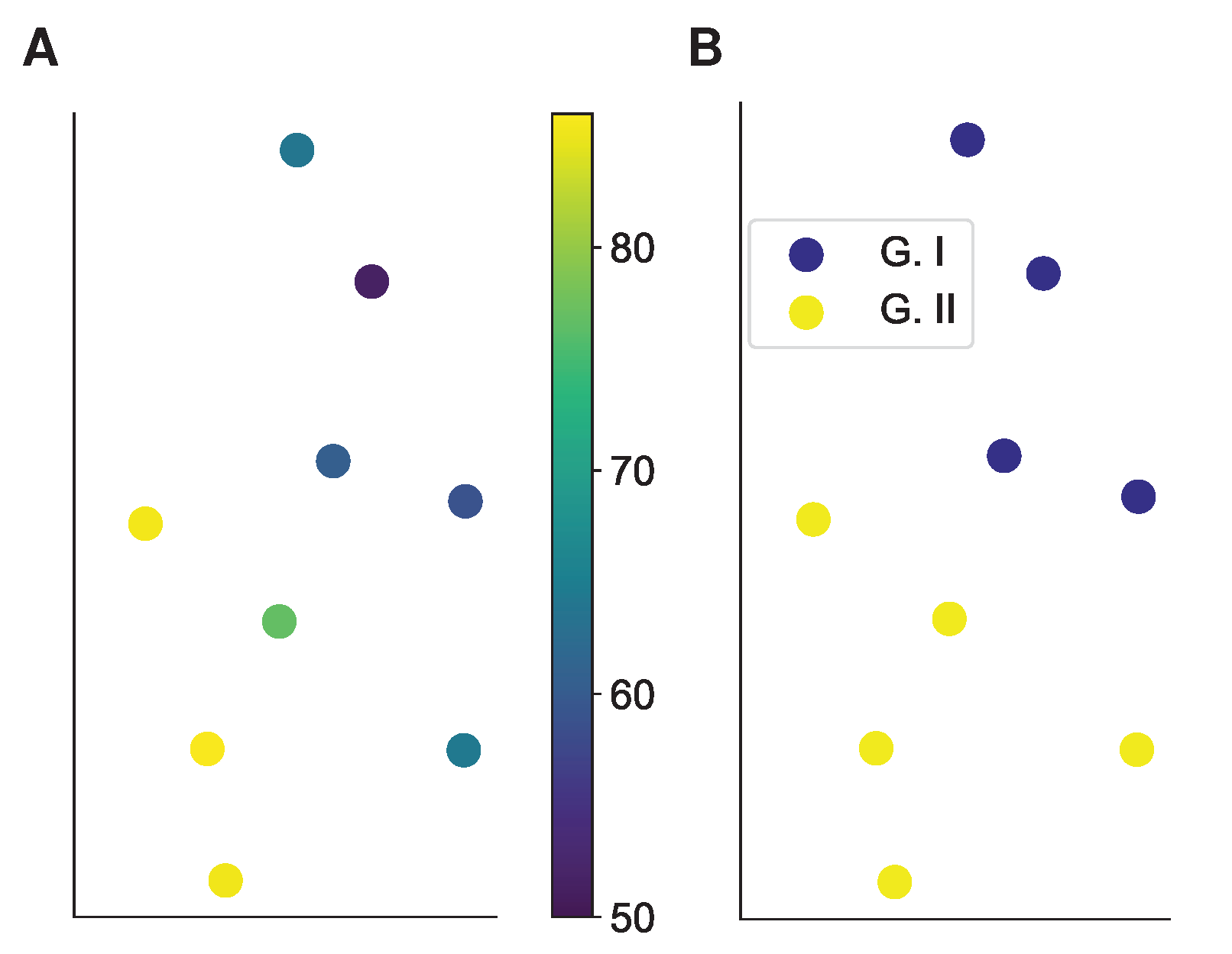
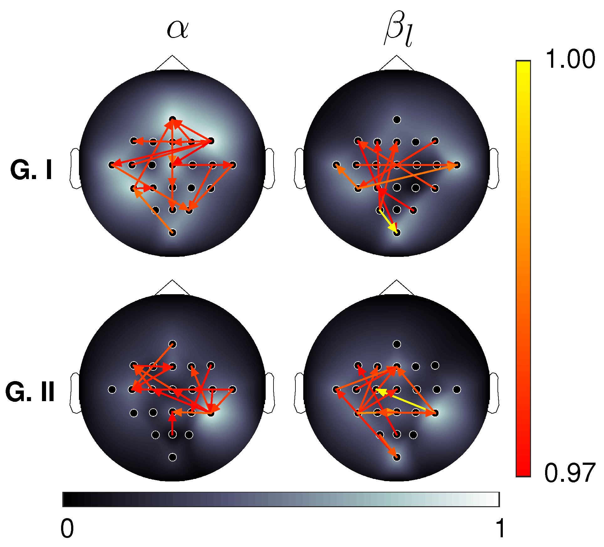
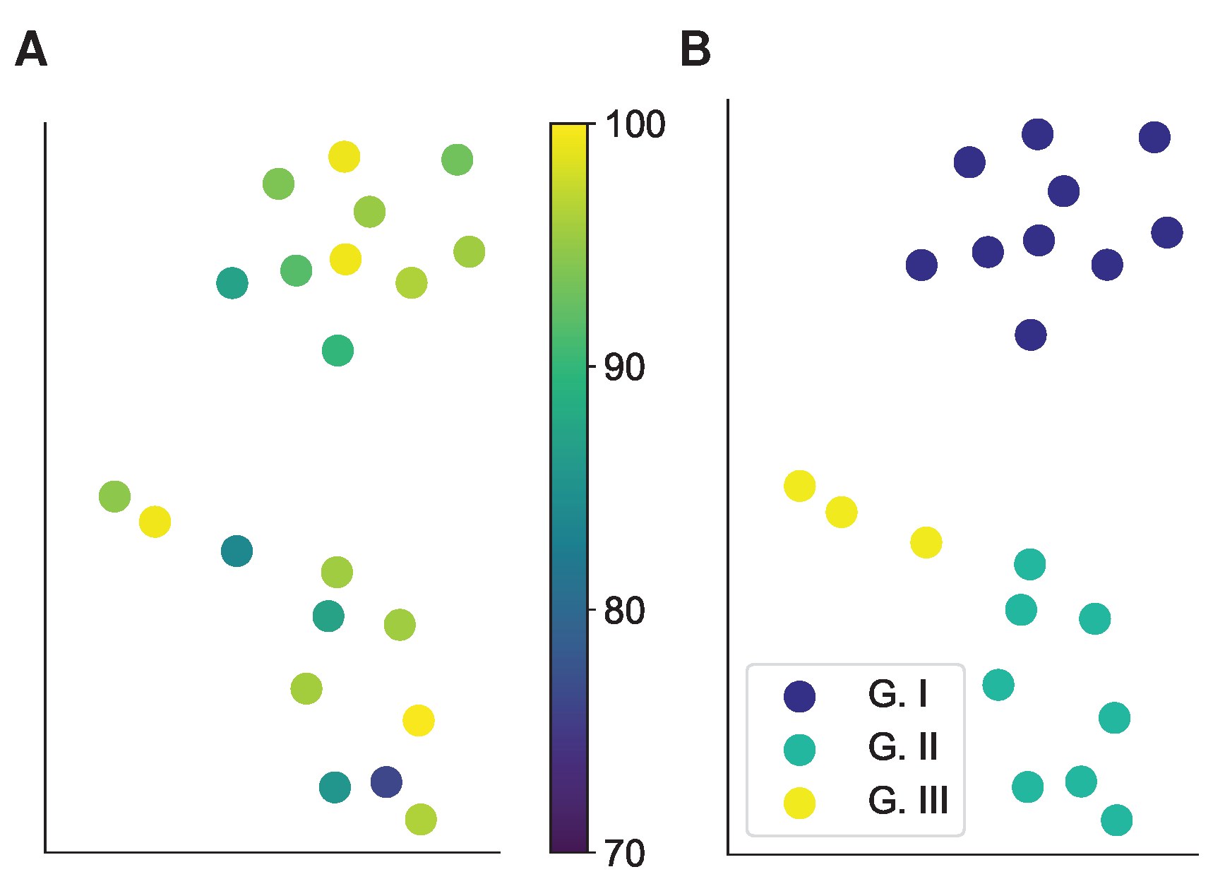
4.2.2. Working Memory Results

Figure 10 presents the average classification accuracy for all subjects in the WM database as a function of the number of selected features, for TE${}_{\kappa \alpha }$ and TE${}_{\kappa \alpha }^{\theta }$. The results show that the classifier trained from phase TE features markedly outperforms the one trained using real-valued TE estimates, as long as the appropriate percentage of features is selected. This difference might be attributed to the hypothesized phase-based nature of directed interactions during WM tasks [35,50], which would be better captured by phase TE. Furthermore, both accuracy curves highlight the importance of feature selection, since they show a steep performance degradation as more features are used to train the classifiers. In this case, the CKA-based relevance analysis not only allows reducing the number of features needed to successfully classify the three cognitive load levels present in the WM data but also prevents the classifiers from being confounded by connections that do not hold relevant information to discriminate between the target conditions.

Figure 11 depicts the highest average classification accuracy per subject for TE${}_{\kappa \alpha }^{\theta }$, GC${}^{\theta }$ and PSI. The subjects are ordered from highest to lowest performance. Unlike the results obtained for the MI database, we do not observe an underperforming group of subjects, especially after considering the fact that for the WM database the classifiers must discriminate among three classes instead of two. On the other hand, in this case, the TE${}_{\kappa \alpha }^{\theta }$-based classifier largely outperforms those based on alternative connectivity estimation strategies in most subjects. Here, we must point out that the auxiliary cross-validation step introduced for feature selection, aiming to obtain stable CKA results for the reduced number of available trials, leads to data leakage. This is because, ultimately, it requires all the available data to estimate $\overline{\mathbf{\varrho }}$, which renders it a nonviable approach for practical BCI implementations and can inflate performance evaluations, such as the accuracy results previously discussed. However, since the same strategy was implemented for all classification systems and connectivity measures considered for the WM database, comparisons among them remain valid, and the relative differences in performance are still informative.

In order to elucidate the pairwise connectivities, and their corresponding frequency bands, that allow the TE${}_{\kappa \alpha }^{\theta }$-based classification system to successfully discriminate among different memory loads, we proceeded as described in Section 4.2.1 and from $\overline{\mathbf{\varrho }}$ obtained a node relevance vector ${\overline{\varrho }}_n\in {\mathbb{R}}^{3C}$. Then, we applied t-SNE on ${\overline{\varrho }}_n$. Figure 12A shows the obtained two-dimensional representation of the relevance vectors for each subject in the WM database. Unlike the results observed before for the MI database, there is not a clear association between the subject distribution on the plot and their classification accuracies. Nonetheless, Figure 12A shows the presence of well-defined groups sharing similar relevance patterns. As before, we grouped the subjects into clusters using the k-means algorithm. The number of clusters was selected as three by visual inspection of the t-SNE results. Figure 12B displays the three groups, termed G. I, G. II, and G. III. The TE${}_{\kappa \alpha }^{\theta }$-based classifier has average accuracies of $0.94\pm 0.04$, $0.92\pm 0.08$, and $0.93\pm 0.08$ for the subjects in G. I, G. II, and G. III, respectively.

Lastly, Figure 13 shows the average nodal relevance, as defined by ${\mathbf{\varrho }}_n$, and the most relevant connectivities for each group, discriminated by frequency band. For G. I we observe widespread high node relevance in both the $\alpha$ and ${\beta }_l$ bands and low node relevance in the $\theta$ band. Most relevant connections are present in the ${\beta }_l$ band with many connections originating in the parieto-occipital region and targeting frontal and centro-frontal areas. For G. II and G. III node relevance is more evenly distributed across the three frequency bands considered. Spatially, it is more prominent around some pre-frontal, frontal, centro-parietal, and parietal nodes. In terms of the most relevant connections, we observe long-range contralateral interactions involving mostly the regions previously listed, as well as some connections to and from temporal areas. Therefore, we argue that the information flow between frontal, parietal, and temporal regions, coded in the phases of oscillatory activity in the $\theta$, $\alpha$, and ${\beta }_l$ bands, is what allowed us to discriminate among different memory loads from TE${}_{\kappa \alpha }^{\theta }$ features. These results agree with several studies that identify fronto-parietal and fronto-temporal neural circuits operating in frequency ranges spanning from $\theta$ to $\beta$ as key during the activation of working memory [35,50,51].

4.3. Limitations

In this study, we employed Morlet wavelets as filters for instantaneous phase extraction prior to phase TE estimation, as proposed in [8]. However, as discussed by the authors in [8], the choice of filter can influence the behavior of phase TE. This is an aspect we have yet to explore for our proposal. In the same line, in [42] the authors showed, using the Kraskov-Stögbauer-Grassberger TE estimator on real-valued filtered signals, that filtering and downsampling are deleterious for TE, since they can lead to altered time delays and hide certain causal interactions. Furthermore, from a conceptual perspective, while filtering dampens spectral power, it does not always remove the information contained in specific frequencies [25]. This would hinder the isolation of frequency specific interactions in TE estimates from real-valued filtered data, the most common approach to obtain spectrally resolved TE values. Whether those effects are also present in the case of phase TE is yet to be analyzed; however, as pointed out in [25], phase TE is conceptually different from spectrally resolved TE. Additionally, the results obtained with our phase TE estimator for the NMM data closely follow those obtained with the PSI, a measure that does not rely on data filtering, which points to a certain degree of robustness to the negative effects that might be associated with phase extraction through complex filtering. A related issue is the possible effects on our proposal of the preprocessing pipelines employed on the EEG data, which involve spectral and spatial filtering. Regarding the former, we have not studied its effects in this work; while for the latter, surface Laplacian positively impacted the discrimination capability of the connectivity features obtained from the different measures considered.

In addition, we are yet to examine the effects of the parameter $\alpha$ in Renyi’s entropy on the proposed phase TE estimator. In [10], we showed that the choice of $\alpha$ indeed modified the performance of the TE${}_{\kappa \alpha }$. The same must hold true for TE${}_{\kappa \alpha }^{\theta }$. Additionally, we selected the autocorrelation time and Cao’s criterion to obtain the embedding parameters for all the TE estimation methods. More complex approaches such as time-delayed mutual information and Ragwitz criterion may yield better results [34]. However, since our motivation was to propose a single-trial phase TE estimator suited as characterization method for BCI applications, the choice of simple parameter estimation methods is justified. As a matter of fact, a practical implementation of a phase TE-based BCI system would likely require further simplifications regarding parameter estimation, in order to facilitate the computation of phase TE in real time. Furthermore, our proposed phase TE estimator inherits the limitations of TE${}_{\kappa \alpha }$ [10]. Namely, it is ill suited to analyze long time series (several thousands of data points) because of the increase in computational cost, especially for non-integer values of the parameter $\alpha$. In addition, it assumes stationary or weakly non-stationary data. Finally, since the definition of causality underlying TE is observational, the proposed phase TE estimator is blind to unobserved common causes, including those resulting from different driving delays.

5. Conclusions

In this work, we proposed a single-trial phase TE estimator. Our method combines a kernel-based TE estimation approach, which defines effectivity connectivity as a linear combination of Renyi’s entropy measures of order $\alpha$, with instantaneous phase time series extracted from the data under analysis. We tested the performance of our proposal on synthetic data generated through NMMs and on two EEG databases obtained under MI and WM paradigms. We compared it with commonly used single-trial TE estimators, applied to phase time series, and the PSI and GC. Our results show that the proposed phase TE estimator successfully detects the direction of interaction between individual pairs of signals, capturing the differences in coupling strength and displaying statistically significant results around the frequencies corresponding to the main oscillatory components present in the data. It also succeeds in detecting bidirectional interactions of localized frequency content and is robust to realistic noise and signal mixing levels. Moreover, our method, coupled with a CKA-based relevance analysis, revealed discriminant spatial and frequency-dependent patterns for both the MI and WM databases, leading to improved classification performance compared with approaches based on real-valued TE estimation. In all our experiments, the proposed single-trial kernel-based phase TE estimator is competitive with the comparison methods previously listed in terms of the performance assessment metrics employed.

As future work, we will look into developing a cross-spectral representation for our phase TE estimator to study directed interactions between oscillations of different frequencies [65]. We will also explore the effects of the choice of filter on the proposed estimator as well as those of the parameters involved in time embedding and in our kernel-based TE estimation approach.

References

1. La Tour, T.D.; Tallot, L.; Grabot, L.; Doyère, V.; Van Wassenhove, V.; Grenier, Y.; Gramfort, A. Non-linear auto-regressive models for cross-frequency coupling in neural time series. PLoS Comput. Biol. 2017, 13, e1005893. [Google Scholar]
2. Da Silva, F.L. EEG: Origin and measurement. In EEg-fMRI; Springer: Berlin/Heidelberg, Germany, 2009; pp. 19–38. [Google Scholar]
3. Wianda, E.; Ross, B. The roles of alpha oscillation in working memory retention. Brain Behav. 2019, 9, e01263. [Google Scholar] [CrossRef] [PubMed] [Green Version]
4. Hyafil, A.; Giraud, A.L.; Fontolan, L.; Gutkin, B. Neural cross-frequency coupling: Connecting architectures, mechanisms, and functions. Trends Neurosci. 2015, 38, 725–740. [Google Scholar] [CrossRef] [PubMed]
5. Xie, P.; Pang, X.; Cheng, S.; Zhang, Y.; Yang, Y.; Li, X.; Chen, X. Cross-frequency and iso-frequency estimation of functional corticomuscular coupling after stroke. Cogn. Neurodyn. 2021, 15, 439–451. [Google Scholar] [CrossRef] [PubMed]
6. Ahmadi, A.; Davoudi, S.; Behroozi, M.; Daliri, M.R. Decoding covert visual attention based on phase transfer entropy. Physiol. Behav. 2020, 222, 112932. [Google Scholar] [CrossRef]
7. Kang, H.; Zhang, X.; Zhang, G. Phase permutation entropy: A complexity measure for nonlinear time series incorporating phase information. Phys. A Stat. Mech. Appl. 2021, 568, 125686. [Google Scholar] [CrossRef]
8. Lobier, M.; Siebenhühner, F.; Palva, S.; Palva, J.M. Phase transfer entropy: A novel phase-based measure for directed connectivity in networks coupled by oscillatory interactions. Neuroimage 2014, 85, 853–872. [Google Scholar] [CrossRef]
9. Sakkalis, V. Review of advanced techniques for the estimation of brain connectivity measured with EEG/MEG. Comput. Biol. Med. 2011, 41, 1110–1117. [Google Scholar] [CrossRef]
10. De La Pava Panche, I.; Alvarez-Meza, A.M.; Orozco-Gutierrez, A. A data-driven measure of effective connectivity based on Renyi’s α-entropy. Front. Neurosci. 2019, 13, 1277. [Google Scholar] [CrossRef] [PubMed]
11. Cekic, S.; Grandjean, D.; Renaud, O. Time, frequency, and time-varying Granger-causality measures in neuroscience. Stat. Med. 2018, 37, 1910–1931. [Google Scholar] [CrossRef]
12. Nolte, G.; Ziehe, A.; Nikulin, V.V.; Schlögl, A.; Krämer, N.; Brismar, T.; Müller, K.R. Robustly estimating the flow direction of information in complex physical systems. Phys. Rev. Lett. 2008, 100, 234101. [Google Scholar] [CrossRef] [PubMed] [Green Version]
13. Jiang, H.; Bahramisharif, A.; van Gerven, M.A.; Jensen, O. Measuring directionality between neuronal oscillations of different frequencies. Neuroimage 2015, 118, 359–367. [Google Scholar] [CrossRef]
14. Schreiber, T. Measuring information transfer. Phys. Rev. Lett. 2000, 85, 461. [Google Scholar] [CrossRef] [PubMed] [Green Version]
15. Zhu, J.; Bellanger, J.J.; Shu, H.; Le Bouquin Jeannès, R. Contribution to transfer entropy estimation via the k-nearest-neighbors approach. Entropy 2015, 17, 4173–4201. [Google Scholar] [CrossRef] [Green Version]
16. Wilmer, A.; de Lussanet, M.; Lappe, M. Time-delayed mutual information of the phase as a measure of functional connectivity. PLoS ONE 2012, 7, e44633. [Google Scholar] [CrossRef]
17. Numan, T.; Slooter, A.J.; van der Kooi, A.W.; Hoekman, A.M.; Suyker, W.J.; Stam, C.J.; van Dellen, E. Functional connectivity and network analysis during hypoactive delirium and recovery from anesthesia. Clin. Neurophysiol. 2017, 128, 914–924. [Google Scholar] [CrossRef]
18. Hillebrand, A.; Tewarie, P.; Van Dellen, E.; Yu, M.; Carbo, E.W.; Douw, L.; Gouw, A.A.; Van Straaten, E.C.; Stam, C.J. Direction of information flow in large-scale resting-state networks is frequency-dependent. Proc. Natl. Acad. Sci. USA 2016, 113, 3867–3872. [Google Scholar] [CrossRef] [PubMed] [Green Version]
19. Wang, S.; Zhang, D.; Fang, B.; Liu, X.; Yan, G.; Sui, G.; Huang, Q.; Sun, L.; Wang, S. A Study on Resting EEG Effective Connectivity Difference before and after Neurofeedback for Children with ADHD. Neuroscience 2021, 457, 103–113. [Google Scholar] [CrossRef]
20. Yang, P.; Shang, P.; Lin, A. Financial time series analysis based on effective phase transfer entropy. Phys. A Stat. Mech. Appl. 2017, 468, 398–408. [Google Scholar] [CrossRef]
21. Rathee, D.; Cecotti, H.; Prasad, G. Single-trial effective brain connectivity patterns enhance discriminability of mental imagery tasks. J. Neural Eng. 2017, 14, 056005. [Google Scholar] [CrossRef]
22. Zhang, R.; Li, X.; Wang, Y.; Liu, B.; Shi, L.; Chen, M.; Zhang, L.; Hu, Y. Using brain network features to increase the classification accuracy of MI-BCI inefficiency subject. IEEE Access 2019, 7, 74490–74499. [Google Scholar] [CrossRef]
23. García-Murillo, D.G.; Alvarez-Meza, A.; Castellanos-Dominguez, G. Single-Trial Kernel-Based Functional Connectivity for Enhanced Feature Extraction in Motor-Related Tasks. Sensors 2021, 21, 2750. [Google Scholar] [CrossRef] [PubMed]
24. Chen, X.; Zhang, Y.; Cheng, S.; Xie, P. Transfer spectral entropy and application to functional corticomuscular coupling. IEEE Trans. Neural Syst. Rehabil. Eng. 2019, 27, 1092–1102. [Google Scholar] [CrossRef] [PubMed]
25. Pinzuti, E.; Wollstadt, P.; Gutknecht, A.; Tüscher, O.; Wibral, M. Measuring spectrally-resolved information transfer. PLoS Comput. Biol. 2020, 16, e1008526. [Google Scholar] [CrossRef] [PubMed]
26. Rényi, A. On measures of entropy and information. In Proceedings of the Fourth Berkeley Symposium on Mathematical Statistics and Probability, Volume 1: Contributions to the Theory of Statistics; The Regents of the University of California: California, CA, USA, 1961. [Google Scholar]
27. Principe, J.C. Information Theoretic Learning: Renyi’s Entropy and Kernel Perspectives; Springer Science & Business Media: New York, NY, USA, 2010. [Google Scholar]
28. Giraldo, L.G.S.; Rao, M.; Principe, J.C. Measures of entropy from data using infinitely divisible kernels. IEEE Trans. Inf. Theory 2015, 61, 535–548. [Google Scholar] [CrossRef] [Green Version]
29. Cortes, C.; Mohri, M.; Rostamizadeh, A. Algorithms for learning kernels based on centered alignment. J. Mach. Learn. Res. 2012, 13, 795–828. [Google Scholar]
30. Wibral, M.; Pampu, N.; Priesemann, V.; Siebenhühner, F.; Seiwert, H.; Lindner, M.; Lizier, J.T.; Vicente, R. Measuring information-transfer delays. PLoS ONE 2013, 8, e55809. [Google Scholar] [CrossRef] [PubMed]
31. Vicente, R.; Wibral, M.; Lindner, M.; Pipa, G. Transfer entropy—A model-free measure of effective connectivity for the neurosciences. J. Comput. Neurosci. 2011, 30, 45–67. [Google Scholar] [CrossRef] [PubMed] [Green Version]
32. Takens, F. Detecting strange attractors in turbulence. In Dynamical Systems and Turbulence, Warwick 1980; Springer: Berlin/Heidelberg, Germany, 1981; pp. 366–381. [Google Scholar]
33. Kraskov, A.; Stögbauer, H.; Grassberger, P. Estimating mutual information. Phys. Rev. E 2004, 69, 066138. [Google Scholar] [CrossRef] [Green Version]
34. Lindner, M.; Vicente, R.; Priesemann, V.; Wibral, M. TRENTOOL: A Matlab open source toolbox to analyse information flow in time series data with transfer entropy. BMC Neurosci. 2011, 12, 119. [Google Scholar] [CrossRef] [Green Version]
35. Dimitriadis, S.; Sun, Y.; Laskaris, N.; Thakor, N.; Bezerianos, A. Revealing cross-frequency causal interactions during a mental arithmetic task through symbolic transfer entropy: A novel vector-quantization approach. IEEE Trans. Neural Syst. Rehabil. Eng. 2016, 24, 1017–1028. [Google Scholar] [CrossRef]
36. Barnett, L.; Barrett, A.B.; Seth, A.K. Granger causality and transfer entropy are equivalent for Gaussian variables. Phys. Rev. Lett. 2009, 103, 238701. [Google Scholar] [CrossRef] [Green Version]
37. Liu, W.; Principe, J.C.; Haykin, S. Kernel Adaptive Filtering: A Comprehensive Introduction; John Wiley & Sons: Hoboken, NJ, USA, 2011; Volume 57. [Google Scholar]
38. Fernández-Ramírez, J.; Álvarez-Meza, A.; Pereira, E.; Orozco-Gutiérrez, A.; Castellanos-Dominguez, G. Video-based social behavior recognition based on kernel relevance analysis. Vis. Comput. 2020, 36, 1535–1547. [Google Scholar] [CrossRef]
39. David, O.; Friston, K.J. A neural mass model for MEG/EEG:: Coupling and neuronal dynamics. NeuroImage 2003, 20, 1743–1755. [Google Scholar] [CrossRef]
40. David, O.; Cosmelli, D.; Friston, K.J. Evaluation of different measures of functional connectivity using a neural mass model. Neuroimage 2004, 21, 659–673. [Google Scholar] [CrossRef] [PubMed]
41. Ursino, M.; Ricci, G.; Magosso, E. Transfer Entropy as a Measure of Brain Connectivity: A Critical Analysis With the Help of Neural Mass Models. Front. Comput. Neurosci. 2020, 14, 45. [Google Scholar] [CrossRef]
42. Weber, I.; Florin, E.; Von Papen, M.; Timmermann, L. The influence of filtering and downsampling on the estimation of transfer entropy. PLoS ONE 2017, 12, e0188210. [Google Scholar] [CrossRef] [Green Version]
43. Collazos-Huertas, D.; Álvarez-Meza, A.; Acosta-Medina, C.; Castaño-Duque, G.; Castellanos-Dominguez, G. CNN-based framework using spatial dropping for enhanced interpretation of neural activity in motor imagery classification. Brain Inform. 2020, 7, 1–13. [Google Scholar] [CrossRef] [PubMed]
44. Tangermann, M.; Müller, K.R.; Aertsen, A.; Birbaumer, N.; Braun, C.; Brunner, C.; Leeb, R.; Mehring, C.; Miller, K.J.; Mueller-Putz, G.; et al. Review of the BCI competition IV. Front. Neurosci. 2012, 6, 55. [Google Scholar]
45. Perrin, F.; Pernier, J.; Bertrand, O.; Echallier, J. Spherical splines for scalp potential and current density mapping. Electroencephalogr. Clin. Neurophysiol. 1989, 72, 184–187. [Google Scholar] [CrossRef]
46. Cohen, M.X. Comparison of different spatial transformations applied to EEG data: A case study of error processing. Int. J. Psychophysiol. 2015, 97, 245–257. [Google Scholar] [CrossRef] [PubMed]
47. Zhang, D.; Zhao, H.; Bai, W.; Tian, X. Functional connectivity among multi-channel EEGs when working memory load reaches the capacity. Brain Res. 2016, 1631, 101–112. [Google Scholar] [CrossRef] [PubMed]
48. Villena-González, M.; Rubio-Venegas, I.; López, V. Data from brain activity during visual working memory replicates the correlation between contralateral delay activity and memory capacity. Data Brief 2020, 28, 105042. [Google Scholar] [CrossRef] [PubMed]
49. Vogel, E.K.; Machizawa, M.G. Neural activity predicts individual differences in visual working memory capacity. Nature 2004, 428, 748–751. [Google Scholar] [CrossRef] [PubMed]
50. Johnson, E.L.; Adams, J.N.; Solbakk, A.K.; Endestad, T.; Larsson, P.G.; Ivanovic, J.; Meling, T.R.; Lin, J.J.; Knight, R.T. Dynamic frontotemporal systems process space and time in working memory. PLoS Biol. 2018, 16, e2004274. [Google Scholar] [CrossRef] [Green Version]
51. Johnson, E.L.; King-Stephens, D.; Weber, P.B.; Laxer, K.D.; Lin, J.J.; Knight, R.T. Spectral imprints of working memory for everyday associations in the frontoparietal network. Front. Syst. Neurosci. 2019, 12, 65. [Google Scholar] [CrossRef] [PubMed] [Green Version]
52. Pedregosa, F.; Varoquaux, G.; Gramfort, A.; Michel, V.; Thirion, B.; Grisel, O.; Blondel, M.; Prettenhofer, P.; Weiss, R.; Dubourg, V.; et al. Scikit-learn: Machine Learning in Python. J. Mach. Learn. Res. 2011, 12, 2825–2830. [Google Scholar]
53. Cao, L. Practical method for determining the minimum embedding dimension of a scalar time series. Phys. D Nonlinear Phenom. 1997, 110, 43–50. [Google Scholar] [CrossRef]
54. Schölkopf, B.; Smola, A.J.; Bach, F. Learning with Kernels: Support Vector Machines, Regularization, Optimization, and Beyond; MIT Press: Cambridge, MA, USA, 2002. [Google Scholar]
55. Akaike, H. A new look at the statistical model identification. IEEE Trans. Autom. Control 1974, 19, 716–723. [Google Scholar] [CrossRef]
56. Gong, A.; Liu, J.; Chen, S.; Fu, Y. Time–Frequency Cross Mutual Information Analysis of the Brain Functional Networks Underlying Multiclass Motor Imagery. J. Mot. Behav. 2018, 50, 254–267. [Google Scholar] [CrossRef]
57. Debener, S.; Minow, F.; Emkes, R.; Gandras, K.; De Vos, M. How about taking a low-cost, small, and wireless EEG for a walk? Psychophysiology 2012, 49, 1617–1621. [Google Scholar] [CrossRef]
58. Mennes, M.; Wouters, H.; Vanrumste, B.; Lagae, L.; Stiers, P. Validation of ICA as a tool to remove eye movement artifacts from EEG/ERP. Psychophysiology 2010, 47, 1142–1150. [Google Scholar] [CrossRef]
59. Li, D.; Zhang, H.; Khan, M.S.; Mi, F. A self-adaptive frequency selection common spatial pattern and least squares twin support vector machine for motor imagery electroencephalography recognition. Biomed. Signal Process. Control 2018, 41, 222–232. [Google Scholar] [CrossRef]
60. Gómez, V.; Álvarez, A.; Herrera, P.; Castellanos, G.; Orozco, A. Short Time EEG Connectivity Features to Support Interpretability of MI Discrimination. In Iberoamerican Congress on Pattern Recognition; Springer: Cham, Switzerland, 2018; pp. 699–706. [Google Scholar]
61. Elasuty, B.; Eldawlatly, S. Dynamic Bayesian Networks for EEG motor imagery feature extraction. In Proceedings of the 2015 7th International IEEE/EMBS Conference on Neural Engineering (NER), Montpellier, France, 22–24 April 2015; pp. 170–173. [Google Scholar]
62. Liang, S.; Choi, K.S.; Qin, J.; Wang, Q.; Pang, W.M.; Heng, P.A. Discrimination of motor imagery tasks via information flow pattern of brain connectivity. Technol. Health Care 2016, 24, S795–S801. [Google Scholar] [CrossRef] [PubMed] [Green Version]
63. Linderman, G.C.; Steinerberger, S. Clustering with t-SNE, provably. SIAM J. Math. Data Sci. 2019, 1, 313–332. [Google Scholar] [CrossRef] [Green Version]
64. Hétu, S.; Grégoire, M.; Saimpont, A.; Coll, M.P.; Eugène, F.; Michon, P.E.; Jackson, P.L. The neural network of motor imagery: An ALE meta-analysis. Neurosci. Biobehav. Rev. 2013, 37, 930–949. [Google Scholar] [CrossRef] [PubMed]
65. Martínez-Cancino, R.; Delorme, A.; Wagner, J.; Kreutz-Delgado, K.; Sotero, R.C.; Makeig, S. What can local transfer entropy tell us about phase-amplitude coupling in electrophysiological signals? Entropy 2020, 22, 1262. [Google Scholar] [CrossRef] [PubMed]
Figure 1. (A) Schematic representation of a neural mass model. (B) 1 s long unidirectionally coupled time series generated by the model. (C) Average power spectrums peaking in the α and lower β frequency bands.
Applsci 11 06689 g001
Figure 2. (A) Schematic representation of the MI protocol. (B) EEG channel montage used for the acquisition of the MI database.
Applsci 11 06689 g002
Figure 3. (A) Schematic representation of the WM protocol. (B) EEG channel montage used for the acquisition of the WM database.
Applsci 11 06689 g003
Figure 4. Schematic representation of our overall classification setup.
Applsci 11 06689 g004
Figure 5. Obtained results for the experiments performed using simulated data from NMMs. Column (A) shows the average connectivity values obtained for different levels of coupling strength. Column (B) presents the average connectivity values estimated for ideal signals and for signals contaminated with noise and signal mixing. Column (C) displays the average connectivity values obtained for bidirectional narrowband couplings. The rows correspond to each of the net phase-based effective connectivity estimation approaches considered for the aforementioned experiments. Circled values indicate statistically significant results at a Bonferroni-corrected alpha level of 3.3 × 10 4 , according to a permutation test based on randomized surrogate trials.
Applsci 11 06689 g005
Figure 6. Average classification accuracies, and their standard deviations, for all subjects in the MI database as a function of the number features selected to train the classifiers.
Applsci 11 06689 g006
Figure 7. (A) Highest average classification accuracy for each subject in the MI database during the training-validation stage. (B) Accuracies obtained for each subject during the testing stage. The subjects are ordered from highest to lowest performance according to the accuracies obtained for the TE κ α θ -based classifier in the training-validation stage.
Applsci 11 06689 g007
Figure 8. (A) Two-dimensional representation of the relevance vectors for each subject in the MI database obtained after applying t-SNE on ϱ n . (B) Groups identified by k-means. For the TE κ α θ -based classifier the subjects grouped in G. I have an average accuracy of 0.59 ± 0.05 , while those in G. II have an average accuracy of 0.80 ± 0.09 .
Applsci 11 06689 g008
Figure 9. Topoplots of the average node (channel) relevance for each group of clustered subjects and frequency band of interest in the MI database (see Figure 8). The arrows represent the most relevant connectivities for each group. For visualization purposes, only 3% of the connections, those with the highest average relevance values per group, are depicted.
Applsci 11 06689 g009
Figure 10. Average classification accuracies, and their standard deviations, for all subjects in the WM database as a function of the number features selected to train the classifiers.
Applsci 11 06689 g010
Figure 11. Highest average classification accuracy for each subject in the WM database. The subjects are ordered from highest to lowest performance according to the accuracies obtained for the TE κ α θ -based classifier.
Applsci 11 06689 g011
Figure 12. (A) Two-dimensional representation of the relevance vectors for each subject in the WM database obtained after applying t-SNE on ϱ n . (B) Groups identified by k-means. For the TE κ α θ -based classifier the subjects grouped in G. I, have an average accuracy of 0.94 ± 0.04 , while those in G. II and G.III have average accuracies of 0.92 ± 0.08 and 0.93 ± 0.08 , respectively.
Applsci 11 06689 g012
Figure 13. Topoplots of the average node (channel) relevance for each group of clustered subjects and frequency band of interest in the WM database (see Figure 12). The arrows represent the most relevant connectivities for each group. For visualization purposes, only the 1% of the connections, those with the highest average relevance values per group, are depicted.
Applsci 11 06689 g013