1. Introduction
Supply (the
“amount of something ready to be used” [
1]) and demand (
“the fact of customers buying goods... and the amount that they buy” [
1] at a given point in time) are two key elements continually interacting in the market. The ability to accurately forecast future demand enables manufacturers to make operational and strategic decisions on resources (allocation and scheduling of raw material and tooling), workers (scheduling, training, promotions, or hiring), manufactured products (market share increase and production diversification), and logistics for deliveries [
2]. Accurate demand forecasts reduce inefficiencies, such as high stocks or stock shortages, which have a direct impact on the supply chain (e.g., reducing the bullwhip effect [
3,
4]), and prevent a loss of reputation [
5].
There is consensus that greater transparency between related parties helps to mitigate the issues mentioned above [
6,
7]. Such transparency can be achieved through automation and digitalization (e.g., implementing Electronic Data Interchange software), by sharing manufacturing processes’ data, and making it timely available to internal stakeholders and relevant external parties where appropriate [
8]. In addition, the ability to apply intelligence to multiple stages across the supply chain can improve its performance [
9]. Such ability and the capability to get up-to-date information regarding any aspect of the manufacturing plant enable the creation of up-to-date forecasts and provide valuable insights for decision-making.
Multiple authors found that machine learning outperforms statistical methods for demand forecasting [
10,
11]. Machine learning methods can be used to train a single model per target demand or a global model to address them all. When designing the models, it is crucial to consider which data is potentially relevant to such forecasts. Multiple factors may affect the product’s demand. First, it is necessary to understand if the products can be considered inelastic (their demand is not sensitive to price fluctuations), complementary, or be substituted for alternative products. Second, intrinsic product qualities, such as being a perishable or luxury item, or their expected lifetime, may be relevant to demand. Finally, the manufacturer must also consider the kind of market it operates on and the customer expectations. When dealing with demand forecasting in the automotive industry, most authors do not use only demand data but also incorporate data regarding exogenous factors that influence demand.
Demand forecasting has direct consequences on decision-making. As such, forecasts are expected to be accurate so that they can be relied upon. When training machine learning models, more significant amounts of good quality data can help the model better learn patterns and provide more accurate forecasts. This intuition is considered when building global models. On the other side, while for local models, the forecast error is constrained to past data of a single time series, in global models, the forecasting error is influenced by patterns and values observed in other time series, which can lead to greater errors as well. In this work, we explore a strategy to constrain such forecasting errors in global models. Furthermore, providing a greater amount of data should be considered regarding products’ demand and its context. To that end, we enrich the demand data with data from complementary data sources, such as world Gross Domestic Product (GDP), unemployment rates, and fuel prices.
This work compares 21 statistical and machine learning algorithms, building local and global forecasting models. We propose two data pooling strategies to develop global time series models. One of them successfully constrains the global time series models’ forecasting errors. We also propose a set of metrics and criteria for the evaluation of demand forecasts for smooth and erratic demands [
12]. The error bounding data pooling strategy enables us to gain the benefits of training machine learning models on larger amounts of data (increased forecast accuracy) while avoiding anomalous forecasts by constraining the magnitude of maximum forecasting errors. The metrics and evaluation criteria aim to characterize the given forecasts and provide better insight when deciding on the best-performing model. We expect the outcomes of this work to provide valuable insights for the development and assessment of demand forecasting models related to the automotive industry, introducing forecasting models and evaluation strategies previously not found in the scientific literature.
To evaluate the performance of our models, we consider the mean absolute scaled error (MASE) [
13] and the R
2-adjusted (R
2adj) metrics. We compute the uncertainty ranges for each forecast and compare if differences between forecasts are statistically significant by performing a Wilcoxon paired rank test [
14]. Finally, we analyze the proportion of products with forecasting errors below certain thresholds and the proportion of forecasts that result in under-estimates.
The rest of this paper is structured as follows.
Section 2 presents related work.
Section 3 describes the methodology we followed to gather and prepare data, create features, and build and evaluate the demand forecasting models.
Section 4 details the experiments performed and the results obtained. Finally,
Section 5 presents the conclusions and an outline of future work.
2. Related Work
Products’ demand forecasting is a broad topic addressed by many authors in the scientific literature. Different demand patterns require specific approaches to address their characteristics. Multiple authors proposed demand classification schemas to understand which techniques are appropriate for a particular demand type. For example, the work in [
15] focused on demand variance during lead times, while the work in [
16] introduced the concept of average demand interval (ADI), which was later widely adopted.
The work in [
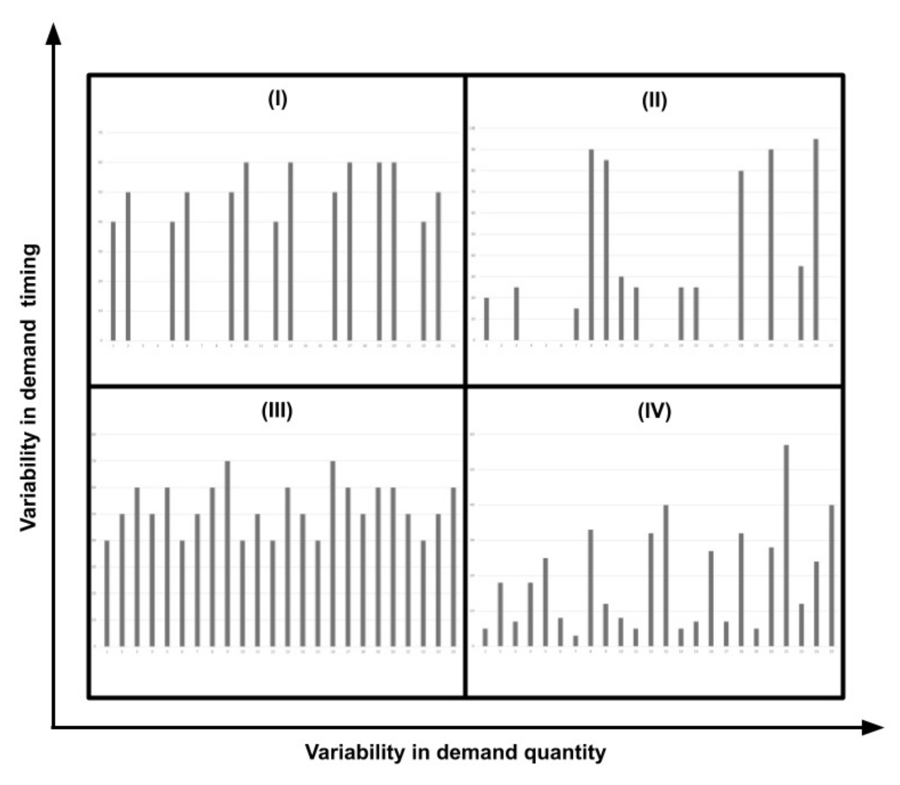
12] complemented this view of demand introducing the coefficient of variation (CV). Both concepts allow us to divide demand types into quadrants, classifying them as intermittent, lumpy, smooth, and erratic demands (see
Figure 1). Smooth and intermittent demand have little variability in demand quantities. Smooth demand has little variability regarding demand intervals over time, while intermittent demand displays a higher demand interval variability. Erratic and lumpy demands have higher variability in demand quantities, which comprehends an additional forecasting model challenge. Erratic demand has little variability regarding demand intervals over time. In lumpy ones, this is an essential factor to be considered. Following demand types proposed in [
12], in this work, we focus on smooth and erratic demands.
Planners, who regularly create demand forecasts, must understand the products they sell, the market they target, the economic context, and customer expectations. Over time they learn how buyers behave, the vast array of factors that can influence product demand, and create their estimates. Each planner can weigh different factors and have distinct ways to ponder them. Most of this information can be collected and fed to machine learning (ML) models, which learn how demand behaves over time to provide a forecast. In the scientific literature addressing demand forecasting in the automotive industry, most authors do not use only demand data, but also incorporate data regarding exogenous factors that influence demand, such as the effect of personal income on car ownership [
17,
18], or the effect of the GDP [
5,
17,
19,
20], inflation rate [
18,
19], unemployment rate [
5], population density [
20], and fuel prices [
5,
18,
20,
21,
22] on vehicles demand.
Demand distributions can also be considered as another source of information for demand forecasting: research performed by many authors confirmed a relationship exists between demand types and demand distributions [
23,
24,
25,
26].
A wide range of models was explored in the literature addressing car, and car components demand forecasting. Ref. [
5] developed a custom additive forecasting model with seasonal, trend, and calendar components. The authors used a phase average to compute the seasonal component, experimented with Multiple Linear Regression (MLR) and Support Vector Machine (SVM) for trend estimation, and used a Linear Regression to estimate the number of working days within a single forecasting period (calendar component). The models were built with car sales data from Germany, obtaining the best results when estimating trends with an SVM model and providing forecasts quarterly. Models’ performance was measured using Mean Absolute Error (MAE) and Mean Absolute Percentage Error (MAPE) metrics. Ref. [
18] compared three models: an adaptive network-based fuzzy inference system (ANFIS), an autoregressive integrated moving average model (ARIMA), and an artificial neural network (ANN). The forecasting models were built considering new automobile monthly sales in Taiwan, obtaining the best results with the ANFIS model. Ref. [
21] developed an ANN model considering the inflation rate, pricing changes in crude oil, and past sales. They trained and evaluated the model on data from the Maruti Suzuki Ltd. company from India, measuring the models’ performance with the Mean Squared Error (MSE) metric. Ref. [
27] compared three models: ANFIS, ANN, and a Linear Regression. They are trained on car sales data from the Maruti car Industry in India and compared with the root mean squared error (RMSE) metric. The authors report that the best performance was obtained with the ANFIS model. Ref. [
28] compared the ARIMA and the Holt–Winters models using demand data regarding remanufactured alternators and starters manufactured by an independent auto parts remanufacturer. They measured performance using the MAPE and average cumulative absolute percentage errors (CAPE) metrics, obtaining the best results for the Holt–Winters models. Ref. [
29] developed three models (ANN, Linear Regression, and Exponential Regression) based on data from the Kia and Hyundai corporations in the US and Canada. Results were measured with the MSE metric, obtaining the best one with the ANN model. Ref. [
19] analyzed the usage of genetic algorithms to tune the parameters from ANFIS models built with data from the Saipa group, a leading automobile manufacturer from Iran. Measuring RMSE and R
2, they achieved the best results with ANFIS models tuned with genetic algorithms compared to ANFIS and ANN models without any tuning. Ref. [
30] compared custom deep learning models trained on real-world products’ data provided by a worldwide automotive original equipment manufacturer (OEM). Ref. [
31] developed an long short-term memory (LSTM) model based on car parts sales data in Norway and compared it against Simple Exponential Smoothing, Croston, Syntetos-Boylan Approximation (SBA), Teunter-Syntetos-Babai, and Modified SBA. Best results were obtained with the LSTM model when comparing models’ mean error (ME) and MSE. Ref. [
22] developed tree models (autoregressive moving average (ARMA), Vector Autoregression (VAR) model, and the Vector Error Correction Model (VECM)) to forecast automobile sales in China. The models were compared based on their performance measured with RMSE and MAPE metrics, finding the best results with the VECM model. The VECM model was also applied by [
20], when forecasting cars demand for the state of Sarawak in Malaysia. Finally, Ref. [
32] compared forecasts obtained from different moving average (MA) algorithms (simple MA, weighted MA, and exponential MA) when applied to production and sales data from the Gabungan Industri Kendaraan Bermotor Indonesia. Considering the Mean Absolute Deviation, the best forecasts were obtained with the Exponential Moving Average.
Additional insights regarding demand forecasting can be found in research related to time series forecasting in other domains. Refs. [
33,
34] described the importance of time series preprocessing regarding trend and seasonality, though [
35,
36] found the ANN models could learn seasonality. The use of local and global forecasting models for time series forecasting was researched in detail by [
35]. Local forecasting models model each time series individually as separate regression problems. In contrast, global forecasting models assume there is enough similarity across the time series to build a single model to forecast them all. Researchers explored the use of global models either clustering time series [
36,
37], or creating a single model for time series that cannot be considered related to each other [
38]. They achieved good performance in both cases.
3. Methodology
To address the demand forecasting problem, we followed a hybrid of the agile and cross-industry standard process for data mining (CRISP-DM) methodologies [
39]. From the CRISP-DM methodology, we took the proposed steps: focus first on understanding the business and the available data, later tackle the data preparation and modeling, and, finally, evaluate the results. We did not follow these steps sequentially, but rather moved several times through them forward and backward, based on our understanding and feedback from end users, as is done in agile methodologies. We describe the work performed in each phase in the following subsections.
3.1. Business Understanding
The automotive industry accounts for one of the largest economies in the world, by revenue [
40]. It is also considered a strong employment multiplier, a characteristic that is expected to grow stronger with the incorporation of complex digital technologies and the fusion with the digital industry [
41]. Environmental concerns have prompted multiple policies and agreements, which foster the development of more environment friendly vehicles and rethinking of current mobility paradigms [
42,
43,
44]. Nevertheless, global vehicle sales and automotive revenue are expected to continue to grow in the future [
45,
46].
Demand forecasting is a critical component to supply chain management as its outcomes directly affect the supply chain and manufacturing plant organization. In our specific case, demand forecasts for the automotive industry engine components worldwide were required on a monthly level, six weeks in advance. In
Section 2, we highlighted related work, data, and techniques used by authors in the automotive industry. On top of data sources suggested in the literature for deriving machine learning features (past demand data, GDP, unemployment rates, and oil price), we incorporated three additional data sources based on experts’ experience: Purchasing Managers’ Index (PMI), copper prices, and sales plans.
PMI is a diffusion index obtained from monthly surveys sent to purchasing managers from multiple manufacturing companies. It summarizes expectations regarding whether the market will expand, contract, or stay the same and how strong the growth or contraction will be.
Prices of the products we forecast are tied to copper price variations used to manufacture them. Therefore, we consider the price of this metal and create derivative features to capture how it influences the products’ price and how it may influence it in the future.
The strategic sales department creates sales plans on a yearly and quarterly basis. Experts consider projected sales to be a good proxy of future demand as they inform buyers’ purchase intentions. We found research that backs their claim (see, e.g., in [
47]), showing that purchase intentions contribute to the forecast’s accuracy. The research done in [
48] shows that purchase intentions are good predictors of future demand for durable products and that this accuracy is higher for short time horizons. Research also shows that the purchase intention bias can be adjusted with past sales data.
Much research was performed on the effect of aggregation on time series [
34,
49,
50,
51], showing that a higher aggregation improves forecast results. Though research shows optimal demand aggregation levels exist [
52], we considered forecasts at a monthly level to reflect business requirements specific to our use case.
To understand demand forecasting models’ desired behavior and performance, we consulted industry experts. They agreed that one-third of demand forecasts produced by planners have up to 30% error, and up to 20% forecasts may have more than 90% error. They also pointed out that 40% of all forecasts result in under-estimates. When issuing a forecast, it is more desirable to have over-estimates than under-estimates. We consider these facts to assess the forecast results.
3.2. Data Understanding
We make use of several data sources when forming features for machine learning, described in
Table 1. We distinguish between internal data sources (non publicly available data regarding a manufacturing company provided by that same company) and external data sources used for the data enrichment process.
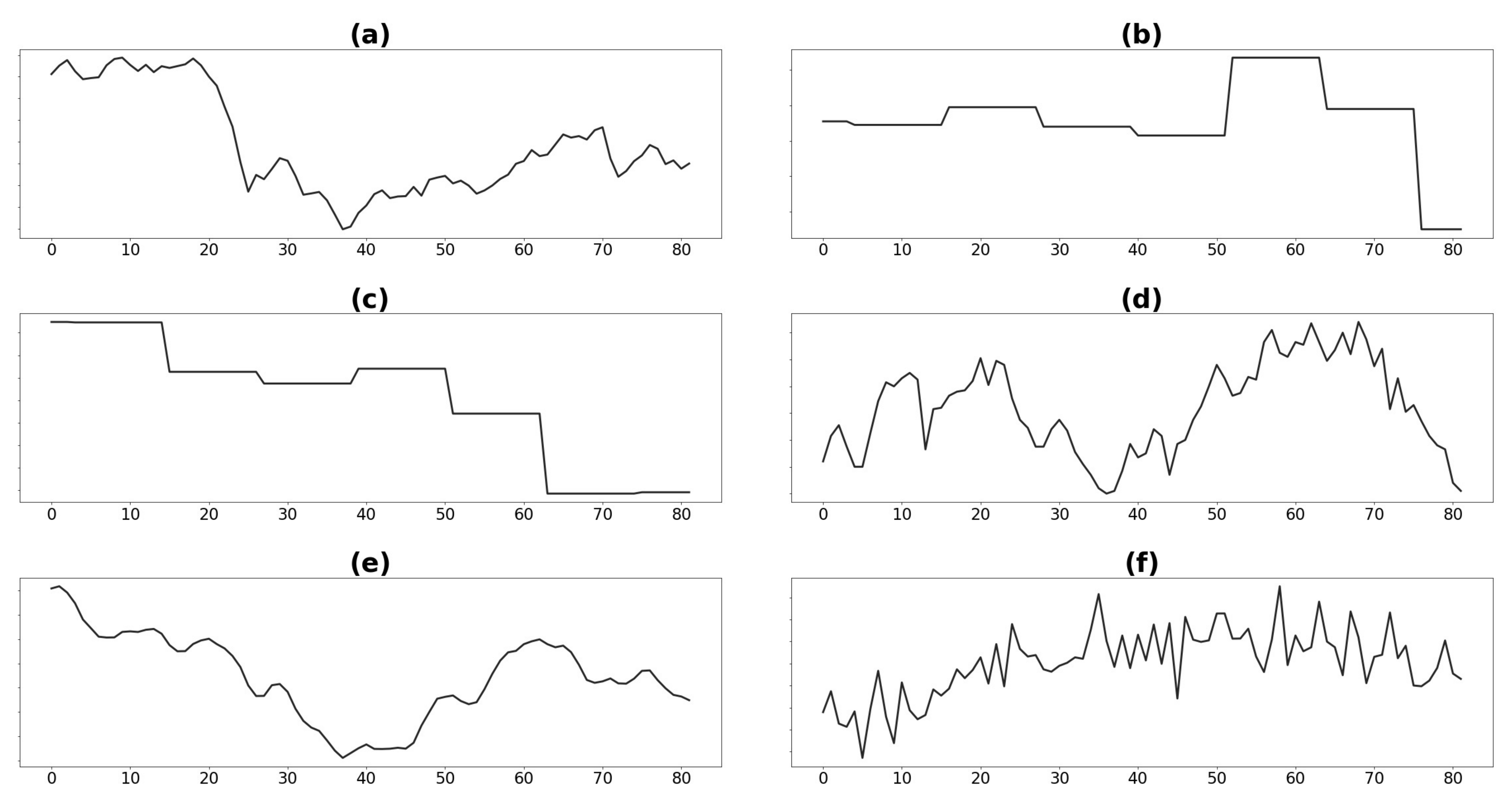
When performing preliminary data analysis over the seven years of data, we found that GDP, crude oil prices, PMI values, and demand (see
Figure 2) show a different pattern before and after the
year 4 of our dataset. When searching for possible root causes, we observed that in
year 4 some significant economic and political events took place affecting the economy worldwide. Among them, we found a stock market crash of a relevant country, a decrease in crude oil production, and several political events that affected the market prospects.
We consider demand quantity as the executed orders of a given product leaving the manufacturing plant on a specific date. Even though demand data is available daily, we aggregate them monthly, satisfying business requirements and providing smoother curves and ease of forecasting. We also consider that months have different working days (due to weekdays and holidays). Thus, we computed the average demand per working day for each month. Future demand can be estimated using the average demand per working day, multiplying by the number of working days in the target month.
Based on the demand classification in [
12], we analyzed how many products correspond to erratic and smooth demands. We create features to capture this behavior. We present the products demand segmentation in
Table 2. From the works in [
23,
24,
26,
53], we understand that demands of a given type follow a certain distribution. Thus, most manufacturing companies’ products may have a slightly different demand behavior but share enough characteristics that would reflect common patterns. We observed that demand values for each product follow a geometric distribution.
To discover potential patterns, we made use of different visualizations.
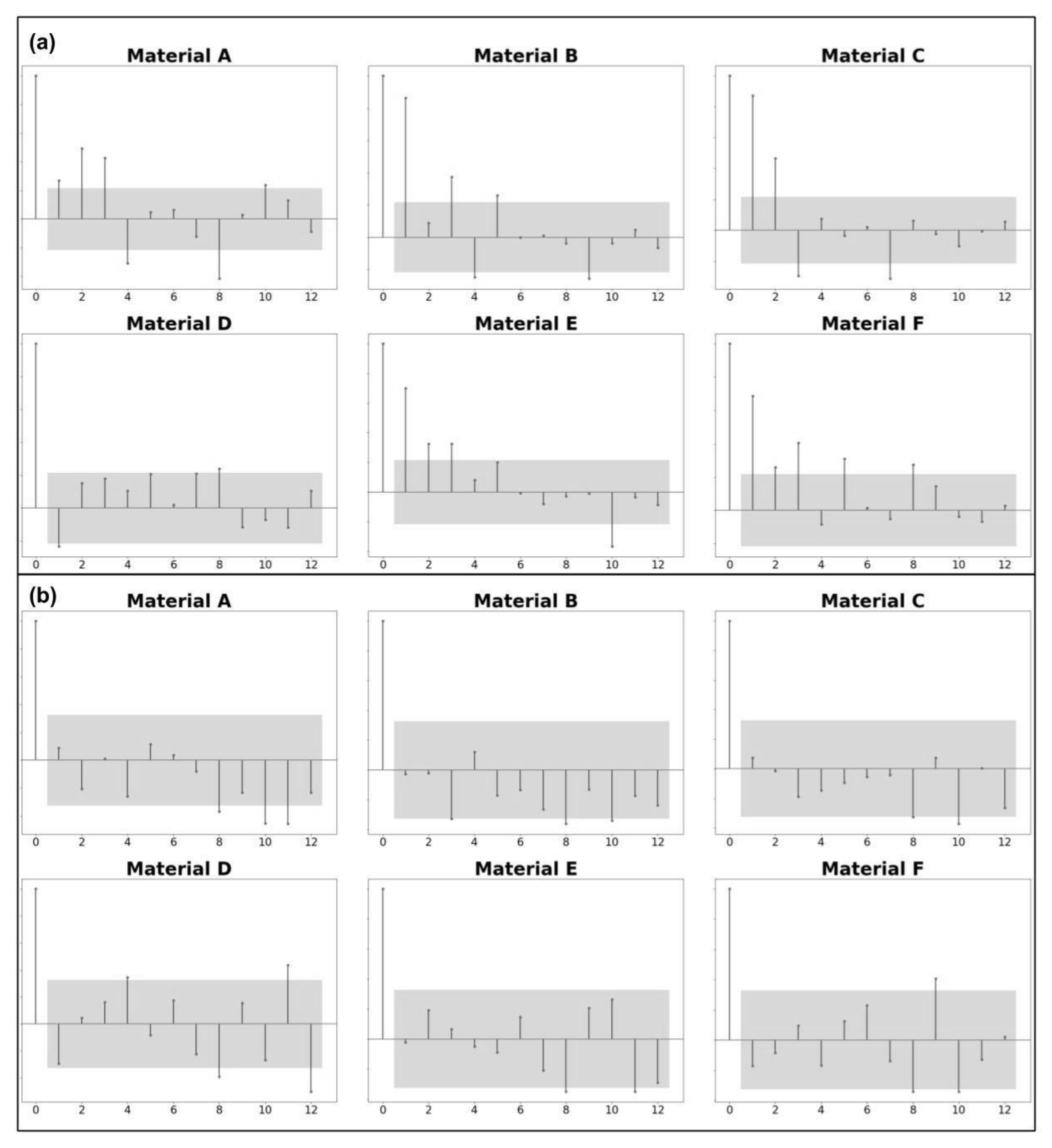
Demand seasonality was assessed with correlograms (see
Figure 3), which show what lags in time most frequently display a statistically significant correlation (with a
p-value = 0.05). Considering all data available, we found the strongest correlations for products at three, four, five, eight, and eleven months before the target month. However, we observed a different pattern in the last three years of data: the strongest correlations occurred at eight, ten, and eleven months before the target. Therefore, we choose only those statistically significant when analyzing correlation values, considering a confidence interval of 95%.
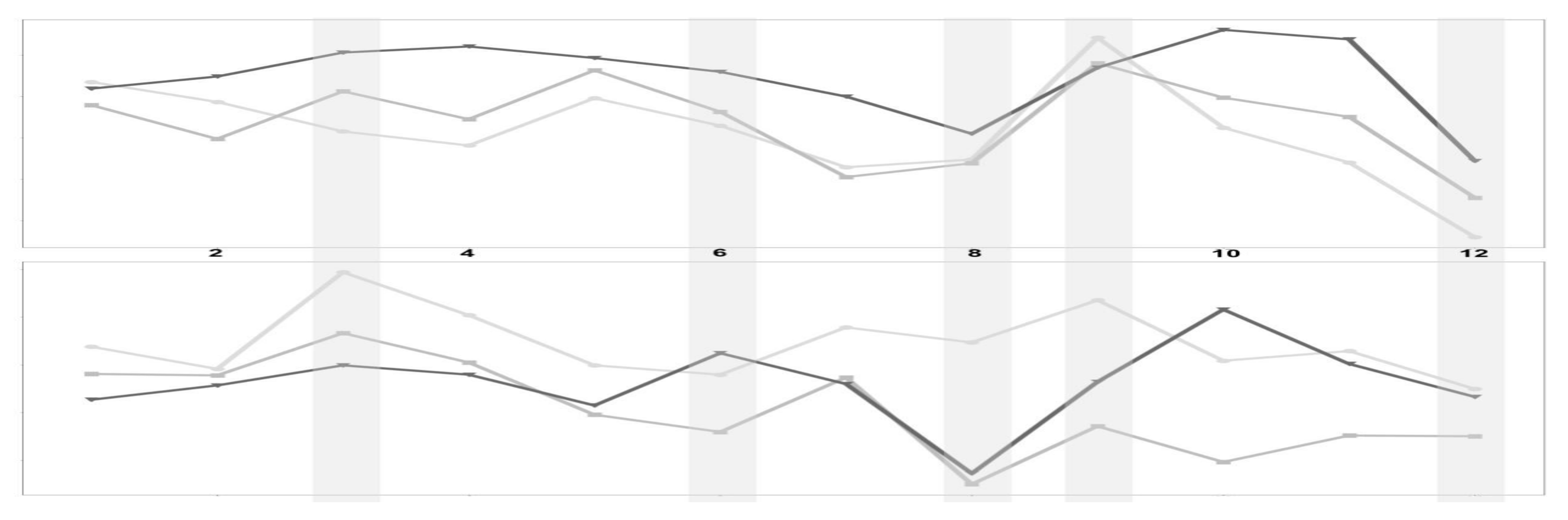
Plotting products’ monthly demand for every year, as shown in
Figure 4, we found that most products were likely to behave similarly over the years for a given month.
When assessing demand data sparsity, we analyzed how many non-zero demand data points we have for each product and the demand magnitudes we observe in each case. We present the data in
Table 2. Higher aggregation levels regarding the time dimension allow reducing variability in time. However, aggregate data at a higher than monthly level are not applicable in our case.
3.3. Data Preparation
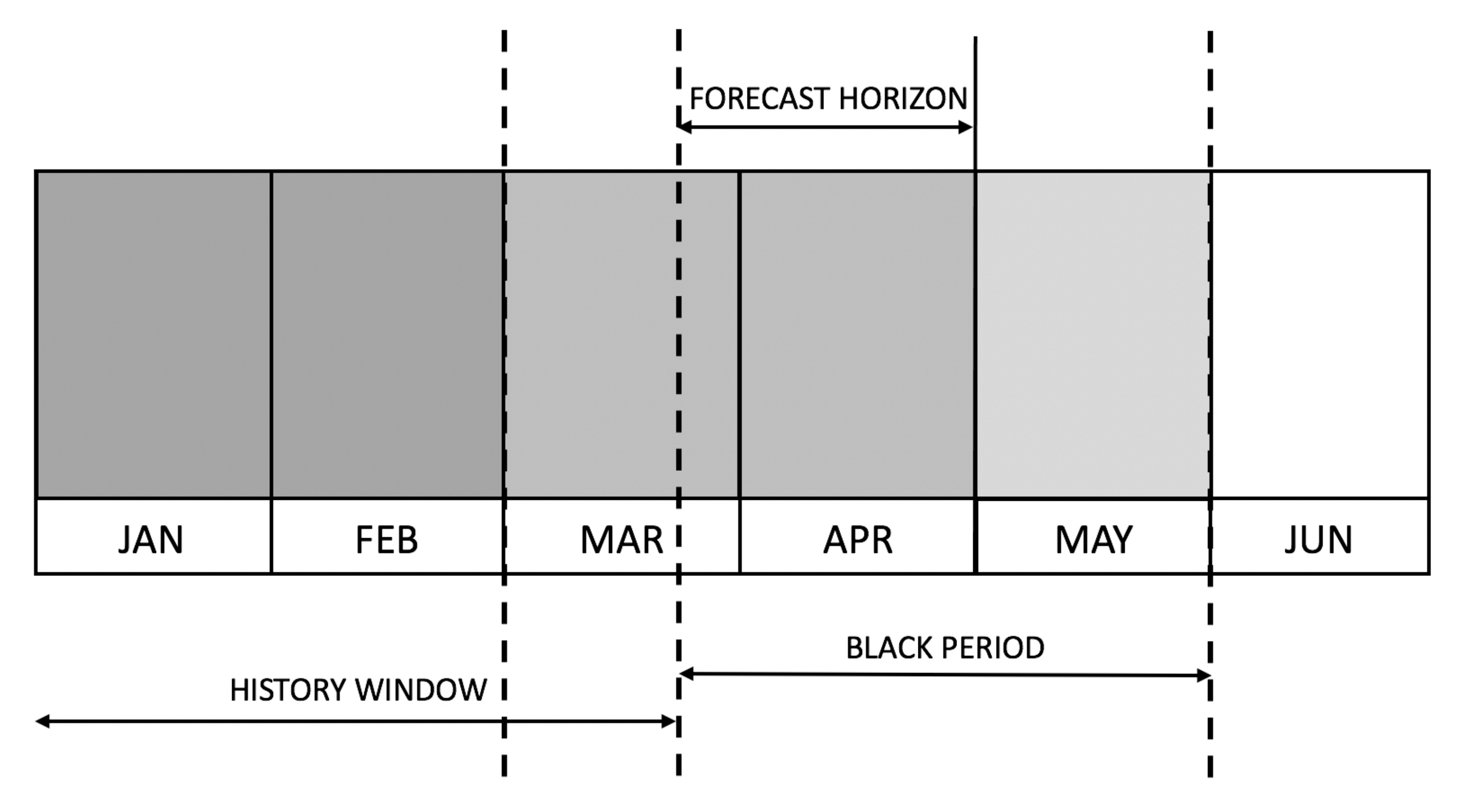
The first step we followed for data preparation was to remove records that would fall into the black period for any given point in time and thus avoid provide our models any indication about the future (except for the target we aim to predict). In our case, we consider a forecasting horizon of six weeks until the beginning of the target month, as depicted in
Figure 5.
For sales plans, we performed data fusion, merging annual and quarterly plans into a single one. In each case, we considered black periods, dates on which each plan becomes available, and the granularity level at which those estimates are provided.
PMI values are informed by the Institute of Supply Chain Management at the beginning of each month, based on the previous month’s survey results. For crude oil prices, we considered the ones provided by the World Bank on a monthly level. We considered the same source for worldwide unemployment rates and GDP values, published yearly and available from March onwards. Every year in early March, the International Organization of Motor Vehicle Manufacturers publishes statistics regarding yearly worldwide car sales, which we used as well. Statistics regarding vehicle production worldwide are incomplete, and thus we did not consider them in this research. For copper prices, we took the London Metal Exchange value for each weekday of the year. We then computed the average price over the last three months. Finally, we computed features based on price adjustments applied to final products based on copper price fluctuations.
All sources of data are merged into a single dataset and aggregated at a product and monthly level.
3.3.1. Feature Creation
We can characterize demand data as a time series per product, each of which may present some level, trend, and seasonality. Therefore, we require a proper assessment of these aspects to create good statistical and ML models. While statistical models use only data regarding past demand to predict the future, ML models can leverage a more extensive set of features. These features provide insights into different factors affecting product demand and are taken into account to make predictions. We created a total of 708 features, some of which we describe below.
We computed rolling summary statistics such as average, maximum, and minimum demand over the last three months to address the time series level. In addition, we computed the same features for a weighted average and minimum and maximum values regarding the target month’s past demand.
Trends help us understand demand growth or contraction and must be considered in forecasting models. However, different approaches may be helpful for statistical and ML models. The statistical models assume that the forecasted time series is stationary. To fulfill this assumption, we applied first-level differencing, which is suitable to address stochastic trends. For ML models, we created features to describe trends and capture monthly or interannual growth or contraction of GDP, unemployment rates, car sales, crude oil, copper prices, and demand. We also created features such as relations between observed demand and sales plans to capture common distortions that may take place on sales plans. Finally, we created derivative features that indicate growth or contraction for given months and more extended periods and detect and tag time series peaks from trend data.
We assessed seasonality using correlograms (see
Figure 3). In addition, we incorporated demand at the lag values described before as proxies of potential demand.
We created naïve features to capture time characteristics to represent the month, a quarter, and workdays for given months. We used information regarding weekdays, national and collective holidays to compute the average demand per workday.
Values such as lagged demands, average, maximum, or minimum value of the last n observed months, and values from sales plans for target month, the weighted average of past demands for target month, and given product could act as reasonable approximations of demand values. Average demand per workday can be used to project expected demand on the target month, multiplying it by the number of workdays in the manufacturing plants. These demand approximations can be further adjusted using trend information.
We created two features to signal demand event occurrence: one based on product data sales plan, and the second one considering values from a probability density function on lagged demand values.
When building a single model for multiple products, it can be helpful to have some features convey information regarding demand similarity. Among others, we provide one-hot encoded features indicating demand-type as described in [
12], considering demand behavior ever since we have data about the product and the last twelve and six months of the point in time we consider. To identify a similar context in which demand occurs, we binned GDP, unemployment rate, crude oil prices, car sales, and demand data into four bins of equal length for each case. Such features may also help identify specific cases, such as
year 4, when context differs from most observed history.
3.3.2. Feature Selection
Feature selection reduces the number of features used to build a model, producing a succinct one that is quick to train, analyze, and understand.
We performed feature selection by combining the manual addition of common sense features with those suggested by a Gradient Boosted Regression Trees (GBRT) model, which is not sensitive to data distribution and allows us to rank features based on how much they reduce variance concerning target values. We only use the data that is later used to train the models and ensure that the test data remains unseen. We performed feature selection to extract the most relevant features in all experiments, considering all products rather than for each product separately. In every case, we selected K features, obtaining K from
, where N is the number of instances in the training subset, as suggested in [
54], and empirically verified these features within our setting. Some of the best features are presented in
Table 3.
3.4. Modeling
Feature Analysis and Prediction Techniques
ML algorithms may have different requirements regarding data preprocessing in order to ensure the best learning conditions. We thus analyzed data distributions and identified which steps were required in each case to satisfy those requirements.
For ML algorithms, we standardized (
3) the features so that they would have zero mean and unit variance Equation (
3), except for the case of the Multiple Linear Perceptron Regressor (MLPR), where we scaled the values of the features between zero and one Equation (
4). Standardization enhances the model’s numerical stability, makes some algorithms consider all features equally important, and shortens ML models’ training times [
55].
We took into account 21 forecasting techniques. We considered the naïve forecast (last observed value as prediction) as the baseline method. We train twelve different batch ML models: on top of MLR, support vector regressor (SVR) [
56], and multilayer perceptron regressor (MLPR) [
57], which we found were used in automotive demand forecasting literature, we also evaluate Ridge [
58]; Lasso [
59]; Elastic Net [
60]; K-nearest-neighbor regressor (KNNR) [
61]; tree-based regressors (decision tree regressor (DTR), random forest regressor (RFR), and GBRT); a voting ensemble created using the most promising and diverse algorithms (KNNR, SVR, and RFR); as well as a stacked regression [
62] considering KNNR, SVR, and RidgeCV as underlying estimators; and a GBRT model as final regressor. We also take into account four streaming ML algorithms: Adaptive Random Forest Regressor (ARFR) [
63], Hoeffding Tree Regressor (HTR) [
64], and Hoeffding Adaptive Tree Regressor (HATR) [
65]. Additionally, we also consider forecasts obtained as the average demand for the last three months (MA(3)) and the ones obtained from statistical forecasting methods (exponential smoothing, random walk, ARIMA(1,1,0), and ARIMA(2,1,0)). We did not create deep learning models since we consider that not enough data was available to train them.
When training the models, we used MSE as the loss function where possible. We choose MSE because it has the desired property of penalizing higher errors more, thus reducing substantial discrepancies in predicted values.
3.5. Evaluation
From the literature review in
Section 2 we observed that authors mostly used ME, MSE, RMSE, CAPE, MAPE, and R
2 metrics to measure the performance of the demand forecasting models related to the automotive industry. While ME, MSE, and RMSE are widely adopted, they all depend on the magnitude of the predicted and observed demands and thus cannot be used to compare groups of products with a different demand magnitude. This issue can be overcome with MAPE or CAPE metrics, though MAPE puts a heavier penalty on negative errors, preferring low forecasts—an undesired property in demand forecasting. Though R
2 is magnitude agnostic, it has been noticed that its value can increase when new features are added to the model [
66].
To evaluate the performance of our models, we consider two metrics: MASE and R2adj. MASE informs the ratio between the MAE of the forecast values against the MAE of the naïve forecast, is magnitude agnostic, and not prone to distortions. R2adj, informs how well predictions adjust to target values. In addition, it weights the number of features used to make the prediction, preferring succinct models that use fewer features for the same forecasting performance.
We compute an uncertainty range for each forecast, which illustrates possible bounds in which future demand values may be found. We also perform the Wilcoxon paired rank test [
14] to assess if forecasts of a given model are significantly better than others.
Summary metrics may not be enough to understand the goodness of fit of a particular model [
67,
68]. Therefore, based on experts’ opinions described in
Section 3, and available demand characterizations, we analyzed the proportion of products with forecasting errors below certain thresholds (5%, 10%, 20%, and 30%), and the proportion of forecasts that resulted in under-estimates.
Though some research highlighted the importance of measuring forecast utility related to inventory performance (see, e.g., in [
69,
70]), this remains out of the scope of this work.
4. Experiments and Results
In this section, we describe the experiments we conducted (summarized in
Table 4) and assess their results with metrics and criteria we described in
Section 3.5. We summarize the outcomes in
Table 5, to understand if a particular model performs significantly better than others. To evaluate the models, we used nested cross-validation [
71], which is frequently used to evaluate time series models. To ensure conditions on ML streaming models were comparable to ML batch models, we implemented the nested cross-validation evaluation strategy. By doing so, we ensured the streaming model did not see new events until the required month was predicted. In order to test the models, we set apart the last six months of data. We published the nested cross-validation implementation for streaming models it in the following repository:
https://github.com/JozefStefanInstitute/scikit-multiflow (accessed date 21 July 2021).
In Experiments 1–4, we assessed how events in year 4 affected model learning and if they significantly degraded forecasts. We also compared two different sets of features, resulting from two different procedures to obtain them. We obtained the best performance with local models trained over the last three years of data. Removing features with high collinearity did not enhance the median of R2adj and MASE. Therefore, we consider Experiment 3 performed best, having the best MASE and R2adj values. In contrast, the rest of the evaluation criteria values were acceptable.
Next, we analyzed if grouping products by specific criteria would enhance the quality of the predictions. We trained these global models over the last three years of data, considering insights obtained from Experiments 1–4. Following the ceteris paribus principle, we considered the same features as for Experiment 3. We experimented with grouping products based on the median magnitude of past demand (Experiment 5) and demand-type (Experiment 6). We observed that even though the median of R2adj was lower, and the under-estimates ratio higher, compared to results in previous experiments, the median MASE values decreased by more than 40%. Models based on the median of past demand had the best results in most aspects, including the proportion of forecasts with more than 90% error. Encouraged by these results, we conducted Experiments 7–8, preserving the grouping criteria but adapting the number of features considered according to the amount of data available in each sub-group. In Experiment 7, we grouped them based on the magnitude of the median of past demand. In contrast, in Experiment 8, we grouped products based on demand type. In both cases, we observed that R2adj values and under-estimates ratios improved, and MASE values remained low. We consider the best results were obtained in Experiment 7, which achieved the best values in all evaluation criteria, except for MASE. We ranked models of these two experiments by R2adj, and took the top three. We obtained SVR, voting, and stacking models for Experiment 7 and SVR, voting, and RFR models for Experiment 8. The models from Experiment 8 exhibited lower MASE in all cases, a better ratio of under-estimates, and a better proportion of forecasts with an error ratio higher than 90%. Top 3 models from Experiment 8 remained competitive regarding R2adj and proportion of forecasts with error ratio bounded to 30% or less error.
We assessed the statistical significance of both groups’ models in all the performance aspects mentioned above, at a p-value = 0.05. The models had no significant difference in the same group regarding R2adj and MASE. However, the difference was significant between voting models in both groups for these two metrics. The difference was also significant between the voting model from Experiment 7 and the RFR model from Experiment 8 for the MASE metric. Considering the proportion of forecasts with errors lower than 30%, we observed no differences between both groups’ models. However, differences between SVR and voting models in Experiment 8 were significant. Finally, differences regarding the number of under-estimates were statistically significant between all top three models from Experiment 7 against SVR and RFR models of Experiment 8. For this particular performance aspect, the stacking model from Experiment 7 only achieves significance against the voting model from Experiment 8.
Having explored a wide range of batch ML models, we conducted Experiments 9–10 with streaming ML models, following the same conditions as Experiment 7–8, but creating a global streaming model for each magnitude of the median of past demand demand-type. This experiment aimed to understand the performance of streaming ML models against the widely used ML batch models and confirm if they behaved the same regarding error bounds as models in Experiments 7–8. We found that streaming models based on Hoeffding inequality did not learn well. On the other side, the Adaptive Random Forest Regressor displayed a better performance. While its R2adj was lower than the top 3 models from Experiment 8, it achieved the best MASE in Experiment 10. It also had among best proportion predictions with less than 5%, 10%, 20%, and 30% error or more than 90% error. However, the proportion of under-estimates, a parameter of crucial importance in our use case, hindered these performance results. ML streaming models had among the highest proportions of under-estimates of all created forecasting models. The highest proportion of under-estimates was obtained in ML streaming models based on the Hoeffding inequality, reaching a median of underestimates above 70%.
In Experiments 5–10, we consistently observed global models created considering the magnitude of the median of past demand outperformed those created based on demand-type when considering the proportion of forecasts with an error higher to 90%. On the other side, global models based on demand-type scored better on MASE. However, these differences did not prove statistically significant in most cases when comparing top-ranking models of both groups.
Having explored different ML models, we then trained statistical models for each product considering demand data available for the last three years (Experiment 11) and contrasted results obtained with the top three models from Experiment 8 (see
Table 6). When preparing demand data for the statistical models, we applied differencing to remove stochastic trends. We observed that the ML models outperformed the statistical ones in almost every aspect. R
2adj was consistently low for statistical models, and though their MASE was better compared to the baseline models, ML models performed better. When assessing the ratio of forecasts with less than 30% error, ML models displayed a better performance. We observed the same when analyzing the under-estimates ratio. Even though the random walk had a low under-estimates ratio, the rest of the metrics indicate the random walk model provides poor forecasts. We consider the best overall performers are the SVR, RFR, and GBRT models, which achieved near-human performance in almost every aspect considered in this research. Even though differences regarding R
2adj, MASE, and the ratio of forecasts with less than 30% error are not statistically significant between them in most cases, they display statistically significant differences when analyzing under-estimates.
5. Conclusions
This research compares 21 forecasting techniques (baseline, statistical, and ML algorithms) to provide future demand estimates for an automotive OEM company located in Europe. We use various internal and external data sources that describe the economic context and provide insights on future demand. We considered multiple metrics and criteria to assess forecasting models’ performance (R2adj, MASE, the ratio of forecasts with less than 30% error, and the ratio of forecasts with under-estimates)—all of them magnitude-agnostic. These metrics and criteria allow us to characterize results to be comparable regardless of the underlying data. We also assess the statistical significance of results, something we missed in most related literature.
The obtained results show that grouping products according to their demand patterns or past demand magnitude enhances the performance of ML models. We observed that the best MASE performance was obtained on models created for a group of products with the same demand type. Furthermore, when training global models based on the median of past demand, models usually achieved a better R2adj and a better bound on high forecast errors. However, these values were not always statistically significant.
Our experimental evaluation indicates that the best performing models are SVR, voting ensemble, and RFR trained over product data of the same demand type. The SVR and RFR models achieved near-human performance for the ratio of forecasts under 30% error, and the RFR model scored close to human performance regarding under-estimates. However, none of the models achieved close to human performance on the proportion of forecasts with a high error (more than 90%). How to efficiently detect and bound such cases remains a subject of future research.
When comparing batch and streaming ML models’ performance, we observed that ML batch models displayed a more robust performance. From the streaming algorithms, the ARFR achieved competitive results, except for a high ratio of under-estimates. This critical aspect must not be overlooked. Models based on the Hoeffding inequality did not learn well and had poor performance, and further research is required to understand the reasons hindering these models’ learning process.
Building a single demand forecasting model for multiple products not only drives better performance, but has engineering implications: fewer models need to be trained and deployed into production. The need for regular deployments can be further reduced by using ML streaming models. This advantage gains importance when considering ever shorter forecasting horizons as it avoids the overhead regular model re-trainings and model deployments. We consider timely access to real data and the ability to regularly update machine learning models as factors that enable digital twins’ creation. Such digital twins not only provide accurate forecasts but allow estimating different what-if scenarios of interest.
We envision at least two directions for future work. First, further research is required to develop effective error bounding strategies for demand forecasts. We want to explore the usage of ML anomaly detection methods to identify anomalous forecasts issued by global models and develop strategies to address such anomalies. Second, research is required to provide explanations that inform the context considered by the ML model and models’ forecasted values and uncertainty. We understand that accurate forecasts are a precondition to building users’ trust in a demand forecasting software. Nevertheless, accurate forecasts alone are not enough. ML models explainability is required to help the user understand the reasons behind a forecast, decide if it can be trusted, and gain more profound domain knowledge.
Author Contributions
Conceptualization, J.M.R., B.K., M.Š., B.F. and D.M.; methodology, J.M.R., B.K., M.Š., B.F. and D.M.; software, J.M.R. and B.K.; validation, J.M.R., B.K., M.Š. and B.F.; formal analysis, J.M.R., B.K., M.Š. and B.F.; investigation, J.M.R., M.Š. and B.F.; resources, J.M.R., B.K., M.Š. and B.F.; data curation, J.M.R., B.K., M.Š. and B.F.; writing—original draft preparation, J.M.R.; writing—review and editing, J.M.R., M.Š., B.F. and D.M.; visualization, J.M.R.; supervision, B.F. and D.M.; project administration, M.Š., B.F. and D.M.; funding acquisition, B.F. and D.M. All authors have read and agreed to the published version of the manuscript.
Funding
This work was supported by the Slovenian Research Agency and European Union’s Horizon 2020 program project FACTLOG under grant agreement number H2020-869951.
Institutional Review Board Statement
Not applicable.
Informed Consent Statement
Not applicable.
Data Availability Statement
Not applicable.
Conflicts of Interest
The authors declare no conflict of interest.
Abbreviations
The following abbreviations are used in this manuscript:
| ADI | Average Demand Interval |
| ANFIS | Adaptive Network-based Fuzzy Inference System |
| ANN | Artificial Neural Network |
| ARFR | Adaptive Random Forest Regressor |
| ARIMA | autoregressive integrated moving average model |
| ARMA | Autoregressive Moving Average |
| CAPE | Cumulative Absolute Percentage Errors |
| CRISP-DM | CRoss-Industry Standard Process for Data Mining |
| CV | Coefficient of Variation |
| DTR | Decision Tree Regressor |
| GBTR | Gradient Boosted Regression Trees |
| GDP | Gross Domestic Product |
| HATR | Hoeffding Adaptive Tree Regressor |
| HTR | Hoeffding Tree Regressor |
| KNNR | K-Nearest-Neighbor Regressor |
| MA | Moving Average |
| MAE | Mean Absolute Error |
| MAPE | Mean Absolute Percentage Error |
| MASE | Mean Absolute Scaled Error |
| ME | Mean Error |
| ML | Machine Learning |
| MLPR | Multiple Linear Perceptron Regressor |
| MLR | Multiple Linear Regression |
| MSE | Mean Squared Error |
| OEM | Original Equipment Manufacturer |
| PMI | Purchasing Managers’ Index |
| R2 | Coefficient of determination |
| R2adj | Coefficient of determination - adjusted |
| RFR | Random Forest Regressor |
| RMSE | Root Mean Squared Error |
| SBA | Syntetos–Boylan Approximation |
| SVM | Support Vector Machine |
| SVR | Support Vector Regressor |
| UE | Under-estimates |
| VAR | Vector Autoregression |
| VECM | Vector Error Correction Model |
References
- Cambridge University Press. Cambridge Learner’s Dictionary with CD-ROM; Cambridge University Press: Cambridge, UK, 2007. [Google Scholar]
- Wei, W.; Guimarães, L.; Amorim, P.; Almada-Lobo, B. Tactical production and distribution planning with dependency issues on the production process. Omega 2017, 67, 99–114. [Google Scholar] [CrossRef] [Green Version]
- Lee, H.L.; Padmanabhan, V.; Whang, S. The bullwhip effect in supply chains. Sloan Manag. Rev. 1997, 38, 93–102. [Google Scholar] [CrossRef]
- Bhattacharya, R.; Bandyopadhyay, S. A review of the causes of bullwhip effect in a supply chain. Int. J. Adv. Manuf. Technol. 2011, 54, 1245–1261. [Google Scholar] [CrossRef]
- Brühl, B.; Hülsmann, M.; Borscheid, D.; Friedrich, C.M.; Reith, D. A sales forecast model for the german automobile market based on time series analysis and data mining methods. In Industrial Conference on Data Mining; Springer: Berlin/Heidelberg, Germany, 2009; pp. 146–160. [Google Scholar]
- De Almeida, M.M.K.; Marins, F.A.S.; Salgado, A.M.P.; Santos, F.C.A.; da Silva, S.L. Mitigation of the bullwhip effect considering trust and collaboration in supply chain management: A literature review. Int. J. Adv. Manuf. Technol. 2015, 77, 495–513. [Google Scholar] [CrossRef]
- Dwaikat, N.Y.; Money, A.H.; Behashti, H.M.; Salehi-Sangari, E. How does information sharing affect first-tier suppliers’ flexibility? Evidence from the automotive industry in Sweden. Prod. Plan. Control. 2018, 29, 289–300. [Google Scholar] [CrossRef]
- Martinsson, T.; Sjöqvist, E. Causes and Effects of Poor Demand Forecast Accuracy A Case Study in the Swedish Automotive Industry. Master’s Thesis, Chalmers University of Technology/Department of Technology Management and Economics, Gothenburg, Sweden, 2019. [Google Scholar]
- Ramanathan, U.; Ramanathan, R. Sustainable Supply Chains: Strategies, Issues, and Models; Springer: New York, NY, USA, 2020. [Google Scholar]
- Gutierrez, R.S.; Solis, A.O.; Mukhopadhyay, S. Lumpy demand forecasting using neural networks. Int. J. Prod. Econ. 2008, 111, 409–420. [Google Scholar] [CrossRef]
- Lolli, F.; Gamberini, R.; Regattieri, A.; Balugani, E.; Gatos, T.; Gucci, S. Single-hidden layer neural networks for forecasting intermittent demand. Int. J. Prod. Econ. 2017, 183, 116–128. [Google Scholar] [CrossRef]
- Syntetos, A.A.; Boylan, J.E.; Croston, J. On the categorization of demand patterns. J. Oper. Res. Soc. 2005, 56, 495–503. [Google Scholar] [CrossRef]
- Hyndman, R.J. Another look at forecast-accuracy metrics for intermittent demand. Foresight Int. J. Appl. Forecast. 2006, 4, 43–46. [Google Scholar]
- Wilcoxon, F. Individual comparisons by ranking methods. In Breakthroughs in Statistics; Springer: New York, NY, USA, 1992; pp. 196–202. [Google Scholar]
- Williams, T. Stock control with sporadic and slow-moving demand. J. Oper. Res. Soc. 1984, 35, 939–948. [Google Scholar] [CrossRef]
- Johnston, F.; Boylan, J.E. Forecasting for items with intermittent demand. J. Oper. Res. Soc. 1996, 47, 113–121. [Google Scholar] [CrossRef]
- Dargay, J.; Gately, D. Income’s effect on car and vehicle ownership, worldwide: 1960–2015. Transp. Res. Part Policy Pract. 1999, 33, 101–138. [Google Scholar] [CrossRef]
- Wang, F.K.; Chang, K.K.; Tzeng, C.W. Using adaptive network-based fuzzy inference system to forecast automobile sales. Expert Syst. Appl. 2011, 38, 10587–10593. [Google Scholar] [CrossRef]
- Vahabi, A.; Hosseininia, S.S.; Alborzi, M. A Sales Forecasting Model in Automotive Industry using Adaptive Neuro-Fuzzy Inference System (Anfis) and Genetic Algorithm (GA). Management 2016, 1, 2. [Google Scholar] [CrossRef] [Green Version]
- Ubaidillah, N.Z. A study of car demand and its interdependency in sarawak. Int. J. Bus. Soc. 2020, 21, 997–1011. [Google Scholar] [CrossRef]
- Sharma, R.; Sinha, A.K. Sales forecast of an automobile industry. Int. J. Comput. Appl. 2012, 53, 25–28. [Google Scholar] [CrossRef]
- Gao, J.; Xie, Y.; Cui, X.; Yu, H.; Gu, F. Chinese automobile sales forecasting using economic indicators and typical domestic brand automobile sales data: A method based on econometric model. Adv. Mech. Eng. 2018, 10, 1687814017749325. [Google Scholar] [CrossRef] [Green Version]
- Kwan, H.W. On the Demand Distributions of Slow-Moving Items. Ph.D. Thesis, University of Lancaster, Lancaster, UK, 1991. [Google Scholar]
- Eaves, A.H.C. Forecasting for the Ordering and Stock-Holding of Consumable Spare Parts. Ph.D. Thesis, Lancaster University, Lancaster, UK, 2002. [Google Scholar]
- Syntetos, A.A.; Babai, M.Z.; Altay, N. On the demand distributions of spare parts. Int. J. Prod. Res. 2012, 50, 2101–2117. [Google Scholar] [CrossRef] [Green Version]
- Lengu, D.; Syntetos, A.A.; Babai, M.Z. Spare parts management: Linking distributional assumptions to demand classification. Eur. J. Oper. Res. 2014, 235, 624–635. [Google Scholar] [CrossRef]
- Dwivedi, A.; Niranjan, M.; Sahu, K. A business intelligence technique for forecasting the automobile sales using Adaptive Intelligent Systems (ANFIS and ANN). Int. J. Comput. Appl. 2013, 74, 975–8887. [Google Scholar] [CrossRef]
- Matsumoto, M.; Komatsu, S. Demand forecasting for production planning in remanufacturing. Int. J. Adv. Manuf. Technol. 2015, 79, 161–175. [Google Scholar] [CrossRef]
- Farahani, D.S.; Momeni, M.; Amiri, N.S. Car sales forecasting using artificial neural networks and analytical hierarchy process. In Proceedings of the Fifth International Conference on Data Analytics: DATA ANALYTICS 2016, Venice, Italy, 9–13 October 2016; p. 69. [Google Scholar]
- Henkelmann, R. A Deep Learning based Approach for Automotive Spare Part Demand Forecasting. Master Thesis, Otto von Guericke Universitat Magdeburg, Magdeburg, Germany, 2018. [Google Scholar]
- Chandriah, K.K.; Naraganahalli, R.V. RNN/LSTM with modified Adam optimizer in deep learning approach for automobile spare parts demand forecasting. Multimed. Tools Appl. 2021, 1–15. [Google Scholar] [CrossRef]
- Hanggara, F.D. Forecasting Car Demand in Indonesia with Moving Average Method. J. Eng. Sci. Technol. Manag. 2021, 1, 1–6. [Google Scholar]
- Zhang, G.P.; Qi, M. Neural network forecasting for seasonal and trend time series. Eur. J. Oper. Res. 2005, 160, 501–514. [Google Scholar] [CrossRef]
- Athanasopoulos, G.; Hyndman, R.J.; Song, H.; Wu, D.C. The tourism forecasting competition. Int. J. Forecast. 2011, 27, 822–844. [Google Scholar] [CrossRef]
- Montero-Manso, P.; Hyndman, R.J. Principles and algorithms for forecasting groups of time series: Locality and globality. arXiv 2020, arXiv:2008.00444. [Google Scholar]
- Salinas, D.; Flunkert, V.; Gasthaus, J.; Januschowski, T. DeepAR: Probabilistic forecasting with autoregressive recurrent networks. Int. J. Forecast. 2020, 36, 1181–1191. [Google Scholar] [CrossRef]
- Bandara, K.; Bergmeir, C.; Smyl, S. Forecasting across time series databases using recurrent neural networks on groups of similar series: A clustering approach. Expert Syst. Appl. 2020, 140, 112896. [Google Scholar] [CrossRef] [Green Version]
- Laptev, N.; Yosinski, J.; Li, L.E.; Smyl, S. Time-series extreme event forecasting with neural networks at uber. In Proceedings of the International Conference on Machine Learning, Sydney, Australia, 6–11 August 2017; Volume 34, pp. 1–5. [Google Scholar]
- Wirth, R.; Hipp, J. CRISP-DM: Towards a standard process model for data mining. In Proceedings of the 4th International Conference on the Practical Applications of Knowledge Discovery and Data Mining; Springer: London, UK, 2000; pp. 29–39. [Google Scholar]
- Wang, C.N.; Tibo, H.; Nguyen, H.A. Malmquist productivity analysis of top global automobile manufacturers. Mathematics 2020, 8, 580. [Google Scholar] [CrossRef] [Green Version]
- Tubaro, P.; Casilli, A.A. Micro-work, artificial intelligence and the automotive industry. J. Ind. Bus. Econ. 2019, 46, 333–345. [Google Scholar] [CrossRef] [Green Version]
- Ryu, H.; Basu, M.; Saito, O. What and how are we sharing? A systematic review of the sharing paradigm and practices. Sustain. Sci. 2019, 14, 515–527. [Google Scholar] [CrossRef] [Green Version]
- Li, M.; Zeng, Z.; Wang, Y. An innovative car sharing technological paradigm towards sustainable mobility. J. Clean. Prod. 2021, 288, 125626. [Google Scholar] [CrossRef]
- Svennevik, E.M.; Julsrud, T.E.; Farstad, E. From novelty to normality: Reproducing car-sharing practices in transitions to sustainable mobility. Sustain. Sci. Pract. Policy 2020, 16, 169–183. [Google Scholar] [CrossRef]
- Heineke, K.; Möller, T.; Padhi, A.; Tschiesner, A. The Automotive Revolution is Speeding Up; McKinsey and Co.: New York, NY, USA, 2017. [Google Scholar]
- Verevka, T.V.; Gutman, S.S.; Shmatko, A. Prospects for Innovative Development of World Automotive Market in Digital Economy. In Proceedings of the 2019 International SPBPU Scientific Conference on Innovations in Digital Economy, Saint Petersburg, Russia, 14–15 October 2019; pp. 1–6. [Google Scholar]
- Armstrong, J.S.; Morwitz, V.G.; Kumar, V. Sales forecasts for existing consumer products and services: Do purchase intentions contribute to accuracy? Int. J. Forecast. 2000, 16, 383–397. [Google Scholar] [CrossRef] [Green Version]
- Morwitz, V.G.; Steckel, J.H.; Gupta, A. When do purchase intentions predict sales? Int. J. Forecast. 2007, 23, 347–364. [Google Scholar] [CrossRef]
- Hotta, L.; Neto, J.C. The effect of aggregation on prediction in autoregressive integrated moving-average models. J. Time Ser. Anal. 1993, 14, 261–269. [Google Scholar] [CrossRef]
- Souza, L.R.; Smith, J. Effects of temporal aggregation on estimates and forecasts of fractionally integrated processes: A Monte-Carlo study. Int. J. Forecast. 2004, 20, 487–502. [Google Scholar] [CrossRef]
- Rostami-Tabar, B.; Babai, M.Z.; Syntetos, A.; Ducq, Y. Demand forecasting by temporal aggregation. Nav. Res. Logist. (NRL) 2013, 60, 479–498. [Google Scholar] [CrossRef]
- Nikolopoulos, K.; Syntetos, A.A.; Boylan, J.E.; Petropoulos, F.; Assimakopoulos, V. An aggregate–disaggregate intermittent demand approach (ADIDA) to forecasting: An empirical proposition and analysis. J. Oper. Res. Soc. 2011, 62, 544–554. [Google Scholar] [CrossRef] [Green Version]
- Syntetos, A.; Babai, M.; Altay, N. Modelling spare parts’ demand: An empirical investigation. In Proceedings of the 8th International Conference of Modeling and Simulation MOSIM, Hammamet, Tunisia, 10–12 May 2010; Citeseer: Forest Grove, OR, USA, 2010; Volume 10. [Google Scholar]
- Hua, J.; Xiong, Z.; Lowey, J.; Suh, E.; Dougherty, E.R. Optimal number of features as a function of sample size for various classification rules. Bioinformatics 2005, 21, 1509–1515. [Google Scholar] [CrossRef] [Green Version]
- Varma, S.; Simon, R. Bias in error estimation when using cross-validation for model selection. BMC Bioinform. 2006, 7, 91. [Google Scholar] [CrossRef] [Green Version]
- Drucker, H.; Burges, C.J.; Kaufman, L.; Smola, A.J.; Vapnik, V. Support vector regression machines. In Proceedings of the Advances in Neural Information Processing Systems, Denver, CO, USA, 2–5 December 1997; pp. 155–161. [Google Scholar]
- Rosenblatt, F. The perceptron: A probabilistic model for information storage and organization in the brain. Psychol. Rev. 1958, 65, 386. [Google Scholar] [CrossRef] [Green Version]
- Hoerl, A.E.; Kennard, R.W. Ridge regression: Biased estimation for nonorthogonal problems. Technometrics 1970, 12, 55–67. [Google Scholar] [CrossRef]
- Tibshirani, R. Regression shrinkage and selection via the lasso. J. R. Stat. Soc. Ser. B 1996, 58, 267–288. [Google Scholar] [CrossRef]
- Zou, H.; Hastie, T. Regularization and variable selection via the elastic net. J. R. Stat. Soc. Ser. B 2005, 67, 301–320. [Google Scholar] [CrossRef] [Green Version]
- Altman, N.S. An introduction to kernel and nearest-neighbor nonparametric regression. Am. Stat. 1992, 46, 175–185. [Google Scholar]
- Wolpert, D.H. Stacked generalization. Neural Netw. 1992, 5, 241–259. [Google Scholar] [CrossRef]
- Gomes, H.M.; Barddal, J.P.; Ferreira, L.E.B.; Bifet, A. Adaptive random forests for data stream regression. In Proceedings of the European Symposium on Artificial Neural Networks, Computational Intelligence and Machine Learning (ESANN), Bruges, Belgium, 2–4 October 2018. [Google Scholar]
- Domingos, P.; Hulten, G. Mining high-speed data streams. In Proceedings of the Sixth ACM SIGKDD International Conference on Knowledge Discovery and Data Mining, Boston, MA, USA, 20–23 August 2000; pp. 71–80. [Google Scholar]
- Bifet, A.; Gavaldà, R. Adaptive learning from evolving data streams. In International Symposium on Intelligent Data Analysis; Springer: New York, NY, USA, 2009; pp. 249–260. [Google Scholar]
- Ferligoj, A.; Kramberger, A. Some Properties of R 2 in Ordinary Least Squares Regression. 1995. [Google Scholar]
- Armstrong, J.S. Illusions in regression analysis. Int. J. Forecast. 2011, 28, 689–694. [Google Scholar] [CrossRef] [Green Version]
- Tufte, E.R. The Visual Display of Quantitative Information; Graphics Press: Cheshire, CT, USA, 2001; Volume 2. [Google Scholar]
- Ali, M.M.; Boylan, J.E.; Syntetos, A.A. Forecast errors and inventory performance under forecast information sharing. Int. J. Forecast. 2012, 28, 830–841. [Google Scholar] [CrossRef]
- Bruzda, J. Demand forecasting under fill rate constraints—The case of re-order points. Int. J. Forecast. 2020, 36, 1342–1361. [Google Scholar] [CrossRef]
- Stone, M. Cross-validatory choice and assessment of statistical predictions. J. R. Stat. Soc. Ser. B 1974, 36, 111–133. [Google Scholar] [CrossRef]
Figure 1.
Demand types classification by Syntetos et al. [
12]. Quadrants correspond to (
I) intermittent, (
II) lumpy, (
III) smooth, and (
IV) erratic demand types.
Figure 1.
Demand types classification by Syntetos et al. [
12]. Quadrants correspond to (
I) intermittent, (
II) lumpy, (
III) smooth, and (
IV) erratic demand types.
Figure 2.
Median values for (a) crude oil price, (b) GDP, (c) unemployment rate worldwide, (d) PMI, (e) copper price (last three months average), and (f) demand.
Figure 2.
Median values for (a) crude oil price, (b) GDP, (c) unemployment rate worldwide, (d) PMI, (e) copper price (last three months average), and (f) demand.
Figure 3.
Sample demand correlograms, indicating seasonality patterns. The correlogram in panel (a) is computed over the seven years of data, while correlogram in (b) is computed over last three years.
Figure 3.
Sample demand correlograms, indicating seasonality patterns. The correlogram in panel (a) is computed over the seven years of data, while correlogram in (b) is computed over last three years.
Figure 4.
Monthly demand over the years of selected products. We compare the last three years of data.
Figure 4.
Monthly demand over the years of selected products. We compare the last three years of data.
Figure 5.
Relevant points in time we considered for forecasting purposes. There is a six-week slot between the moment we issue the forecast and the month we predict. The day of the month considered issuing the prediction is fixed.
Figure 5.
Relevant points in time we considered for forecasting purposes. There is a six-week slot between the moment we issue the forecast and the month we predict. The day of the month considered issuing the prediction is fixed.
Table 1.
Data sources. In the first and second columns, we indicate the kind of data we retrieve and its source. The third column provides information on how frequently new data is available. In contrast, the last column describes the aggregation level at which the data is published. Periodicity and aggregation levels can be at a yearly, quarterly, monthly, or daily level and are denoted by “Y”, “Q”, “M”, or “D”, respectively. The London Metal Exchange published copper prices for weekdays.
| Data | Source | Periodicity | Aggregation Level |
|---|
| History of deliveries | Internal | D | D |
| Sales Plan | Internal | Y,Q | M |
| Gross Domestic Product (GDP) | World Bank | Y | Y |
| Unemployment rate | World Bank | Y | Y |
| Crude Oil price | World Bank | M | M |
| Purchasing Managers’ Index (PMI) | Institute of Supply Chain Management | M | M |
| Copper price | London Metal Exchange | D | D |
| Car sales | International Organization of | Y | Y |
| | Motor Vehicle Manufacturers | | |
Table 2.
Demand segmentations, by demand type as per [
12], and by demand magnitude, considering demanded quantities per month.
Table 2.
Demand segmentations, by demand type as per [
12], and by demand magnitude, considering demanded quantities per month.
| | By Demand Type | By Demand Magnitude |
|---|
| Years | Smooth | Erratic | 10 | 100 | 1 K | 10 K | 100 K |
| All years | 13 | 43 | 13 | 2 | 5 | 26 | 10 |
| Last 3 years | 19 | 37 | 10 | 1 | 4 | 28 | 13 |
Table 3.
Top 15 features selected by the GBRT model considering the last three years of data. We did not remove correlated features in this case.
Table 3.
Top 15 features selected by the GBRT model considering the last three years of data. We did not remove correlated features in this case.
| Feature | Brief Description |
|---|
| Estimate of target demand based on average demand per working day on
third month before predicted month, and amount of working days on target month. |
| Planned sales for target month adjusted with ratio of weighted averages of
past demand and past planned sales for given month. |
| Lagged demand (4 months before target month), adjusted by the ratio of unemployment
rates three, and fifteen months before the month we aim to predict. |
| Planned sales for last year, same month we aim to predict. |
| Planned sales, adjusted by the ratio of unemployment rates three and fifteen
months before the month we aim to predict. |
| Planned sales for target month |
| Lagged demand (3 months before target month), adjusted by the ratio of GDP
three and fifteen months before the month we aim to predict. |
| Planned sales for target month, adjusted by the ratio of GDP three and fifteen months
before the month we aim to predict. |
| Lagged demand (3 months before target month) |
| Estimate of target demand based on average demand per working day a year before
the predicted month and amount of working days on target month. Adjusted by the
the ratio between planned sales for target month and the weighted average of
planned sales for the same month over past years. |
| Estimate of target demand based on average demand per working day on eighth month
before predicted month and amount of working days on target month. |
| An estimate of target demand based on average demand per working day on the fifth month
before predicted month and amount of working days on target month. Adjusted by the
ratio of unemployment rates three and fifteen months
before the month we aim to predict. |
| An estimate of target demand based on average demand per working day a year before
predicted month and the amount of working days on target month. Adjusted by
the ratio between PMI values 13, and 14 months beforethe target month. |
| Lagged demand (3 months before target month) - scaled between 0–1,
considering products past demand values. |
| Estimate of target demand based on average demand per working day on third month
before predicted month, and amount of working days on target month. Adjusted
by the ratio of GDP three and fifteen months before the month we aim to predict. |
Table 4.
Description of experiments performed. Regarding the feature selection procedure, we consider two cases: (I) top features ranked by a GBRT model and curated by a researcher, and (II) top features ranked by a GBRT model, removing those with strong collinearity, curated by a researcher as well. N in the “Number of features” column refers to the number of instances in a given dataset.
| Years of Data | Experiment | Feature Selection | Number of Features |
|---|
| All years available | Experiment 1 | I | 6 |
| Experiment 2 | II | 6 |
| Last three years | Experiment 3 | I | 6 |
| Experiment 4 | II | 6 |
| Experiment 5 | II | 6 |
| Experiment 6 | II | 6 |
| Experiment 7 | II | |
| Experiment 8 | II | |
| Experiment 9 | II | |
| Experiment 10 | II | |
| Experiment 11 | Only past demand | 1 |
Table 5.
Median of results obtained for each ML experiment. We abbreviate under-estimates as UE. In Experiments 9–10, streaming models based on Hoeffding bound show poor performance, resulting in negative R2adj values. We highlight the best results in bold.
Table 5.
Median of results obtained for each ML experiment. We abbreviate under-estimates as UE. In Experiments 9–10, streaming models based on Hoeffding bound show poor performance, resulting in negative R2adj values. We highlight the best results in bold.
| Experiment | R2adj | MASE | 5% Error | 10% Error | 20% error | 30% Error | UE | 90%+ Error |
|---|
| Experiment 1 | 0.8584 | 1.1450 | 0.0670 | 0.1086 | 0.2039 | 0.3051 | 0.3854 | 0.4077 |
| Experiment 2 | 0.8447 | 1.1450 | 0.0655 | 0.1101 | 0.1920 | 0.2887 | 0.4182 | 0.3928 |
| Experiment 3 | 0.9067 | 0.9150 | 0.0655 | 0.1280 | 0.2351 | 0.3095 | 0.4256 | 0.3928 |
| Experiment 4 | 0.8998 | 0.9750 | 0.0655 | 0.1176 | 0.2143 | 0.3051 | 0.4152 | 0.4018 |
| Experiment 5 | 0.8757 | 0.3900 | 0.0536 | 0.1116 | 0.2173 | 0.3140 | 0.4762 | 0.3497 |
| Experiment 6 | 0.8679 | 0.3350 | 0.0565 | 0.1012 | 0.1875 | 0.2768 | 0.4851 | 0.3601 |
| Experiment 7 | 0.8903 | 0.3550 | 0.0521 | 0.1131 | 0.2247 | 0.3155 | 0.4851 | 0.3408 |
| Experiment 8 | 0.8786 | 0.3100 | 0.0506 | 0.0938 | 0.1890 | 0.2813 | 0.4658 | 0.3497 |
| Experiment 9 | −0.1611 | 0.8100 | 0.0357 | 0.0714 | 0.1428 | 0.2143 | 0.7321 | 0.3601 |
| Experiment 10 | −1.5344 | 0.5300 | 0.0178 | 0.0536 | 0.1250 | 0.2143 | 0.7143 | 0.4613 |
Table 6.
Results we obtained for the top 3 performing models from Experiment 8 (ML batch models), best result for experiments 9–10 (ML streaming models), and baseline and statistical models. We abbreviate under-estimates as UE.
Table 6.
Results we obtained for the top 3 performing models from Experiment 8 (ML batch models), best result for experiments 9–10 (ML streaming models), and baseline and statistical models. We abbreviate under-estimates as UE.
| Algorithm Type | Algorithm | R2adj | MASE | 5% Error | 10% Error | 20% Error | 30% Error | UE | 90+% Error |
|---|
| ML batch | SVR | 0.9212 | 0.2600 | 0.0774 | 0.1101 | 0.2321 | 0.3333 | 0.4077 | 0.3304 |
| Voting | 0.9059 | 0.2800 | 0.0625 | 0.0923 | 0.1786 | 0.2798 | 0.4792 | 0.3393 |
| RFR | 0.8953 | 0.2900 | 0.0417 | 0.1012 | 0.2173 | 0.3244 | 0.3423 | 0.3482 |
| ML streaming | ARFR (Experiment 9) | 0.8728 | 0.3300 | 0.0744 | 0.1339 | 0.2500 | 0.3274 | 0.5387 | 0.3452 |
| ARFR (Experiment 10) | 0.8205 | 0.2200 | 0.0744 | 0.1280 | 0.2232 | 0.3274 | 0.5268 | 0.3423 |
| Baseline | MA(3) | 0.8938 | 0.8800 | 0.1190 | 0.1667 | 0.2530 | 0.3482 | 0.3571 | 0.3065 |
| Naïve | 0.8519 | 1.0000 | 0.2024 | 0.2411 | 0.3423 | 0.4137 | 0.4137 | 0.3214 |
| Statistical | ARIMA(2.1.0) | 0.3846 | 0.4500 | 0.0476 | 0.0774 | 0.1429 | 0.1875 | 0.5536 | 0.5208 |
| Exponential smoothing | 0.3258 | 0.3600 | 0.0506 | 0.1161 | 0.1905 | 0.2738 | 0.5923 | 0.4434 |
| ARIMA(1.1.0) | 0.2840 | 0.5200 | 0.0387 | 0.0744 | 0.1012 | 0.1726 | 0.5119 | 0.6071 |
| Random walk | −0.6705 | 0.9000 | 0.0327 | 0.0387 | 0.0655 | 0.0923 | 0.3780 | 0.7678 |
| Publisher’s Note: MDPI stays neutral with regard to jurisdictional claims in published maps and institutional affiliations. |
© 2021 by the authors. Licensee MDPI, Basel, Switzerland. This article is an open access article distributed under the terms and conditions of the Creative Commons Attribution (CC BY) license (https://creativecommons.org/licenses/by/4.0/).


 ,
, 


