Quantitative Monitoring of Dynamic Blood Flows Using Coflowing Laminar Streams in a Sensorless Approach

Abstract

Determination of blood viscosity requires consistent measurement of blood flow rates, which leads to measurement errors and presents several issues when there are continuous changes in hematocrit changes. Instead of blood viscosity, a coflowing channel as a pressure sensor is adopted to quantify the dynamic flow of blood. Information on blood (i.e., hematocrit, flow rate, and viscosity) is not provided in advance. Using a discrete circuit model for the coflowing streams, the analytical expressions for four properties (i.e., pressure, shear stress, and two types of work) are then derived to quantify the flow of the test fluid. The analytical expressions are validated through numerical simulations. To demonstrate the method, the four properties are obtained using the present method by varying the flow patterns (i.e., constant flow rate or sinusoidal flow rate) as well as test fluids (i.e., glycerin solutions and blood). Thereafter, the present method is applied to quantify the dynamic flows of RBC aggregation-enhanced blood with a peristaltic pump, where any information regarding the blood is not specific. The experimental results indicate that the present method can quantify dynamic blood flow consistently, where hematocrit changes continuously over time.

1. Introduction

Blood, which consists of cells (i.e., red blood cells [RBCs], white blood cells, and platelets) as well as plasma proteins, has been considered a two-phase complex fluid. As RBCs constitute 45% of the blood, RBC behaviors have a substantial influence on its flow. Blood behaves as a non-Newtonian fluid at lower shear rates, but as a Newtonian fluid at higher shear rates [1]. It is influenced significantly by hemorheological properties (i.e., viscoelasticity [2,3], hematocrit [4,5], deformability [6,7], and aggregation [8,9]), and vessel geometries (i.e., channel size and cell-free layer). Clinical vascular diseases are characterized by abnormal blood flow or unsteady blood flow [10,11].

Recently, among hemorheological properties, blood viscosity has been considered a promising factor for the early detection of cardiovascular diseases. As blood viscosity varies depending on channel shape or size, the measurement obtained with a conventional viscometer (i.e., cone-and-plate viscometer, parallel-plate viscometer, and capillary viscometer) exhibits substantial differences when compared with the measurement obtained with in vivo blood vessels [12,13]. Since a microfluidic platform with the ability to fabricate blood vessels of similar sizes was introduced, it has been used widely to quantify various hemorheological properties, including viscoelasticity [14,15,16], hematocrit [17,18,19,20,21,22], RBC deformability [21,23,24,25], and RBC aggregation [26,27]. More recently, by connecting a microfluidic chip to a rat model, blood viscosity is monitored at specific intervals [28,29]. While measuring blood viscosity under an in vitro closed loop, the blood flow rate is obtained periodically with micro-particle image velocimetry (PIV) [30].

According to previous studies, several methods for measuring the flow rate of fluids have been demonstrated in microfluidic channels. Borghs et al. reported flow rate measurement of a CaCl₂ solution with electrical impedance [31]. Levy et al. showed a Doppler shift of diffracted light for measuring the velocity of oil bubbles or gas bubbles [32]. Simoni et al. demonstrated small displacement of a Bragg grating on a soft wall for determining the flow rate of water [33]. Hajghassem et al. suggested a cantilever-based optofluidic sensor for measuring the flow rate of water [34]. Walker et al. reported a microcantilever sensor for quantifying the flow rate of water in a paper microfluidic system [35]. Weitz et al. reported fluorescence photobleaching for determining velocity as well as the viscosity of PEG or sucrose [36]. Sanati-Nezhad et al. suggested a microwave-microfluidic resonator for detecting the flow rate of the culture medium (DMEM) [37]. Huang et al. introduced multiple thermistors for measuring the mass flow rate of water and isopropyl alcohol (IPA) [38]. Diamond et al. introduced a check valve for a photo-responsive hydrogel (pNIPPAM) for controlling the flow rate of water [39]. French et al. demonstrated that the flow rate of suspension blood (RBCs in 1× PBS, hematocrit [Hct] = 10–20%) could be quantified with the micro-PIV technique [40]. The blood flow rate obtained with micro-PIV is varied significantly depending on the hematocrit [41]. For example, when aggregation-enhanced blood is circulated in an in vitro loop, the hematocrit of blood is varied continuously over time [30]. When a driving syringe is installed horizontally or vertically, the hematocrit also tends to increase or decrease with time [42]. For this reason, the micro-PIV technique does not provide an accurate flow rate of blood if (1) the hematocrit of blood varies over time or (2) information regarding hematocrit is not available. According to the working principle of blood viscosity, the flow rate of blood should be obtained in advance or controlled. While measuring the blood viscosity, inaccurate information on the blood flow rate results in large measurement errors. To avoid an unexceptional measurement error for quantifying the blood flow rate, it is necessary to replace the blood viscosity with another property (i.e., pressure or work).

As blood pressure is proportional to blood viscosity, it can be used to monitor blood flow instead of blood viscosity. Additionally, blood pressure, which is not affected by RBCs, can be used to monitor the contribution of plasma. Burns et al. introduced pressure sensing with trapped air-liquid compression in a glass microchannel [43]. A glass microchannel is replaced by glass capillaries inserted into the PDMS microchannel channels [44,45]. Kaneko et al. reported an on-chip pressure sensor in terms of color intensity resulting from PDMS channel deformation [46]. Yang et al. suggested a liquid-metal pressure sensor integrated into a microfluidic channel [47]. Blood pressure is monitored with the intensity of RBCs within the big dead channel [48]. As the method is only demonstrated under periodic on-off blood flows, it still shows limitations in the continuous monitoring of blood pressure.

In this study, a coflowing channel as a pressure sensor is suggested to measure blood pressure. Using a coflowing channel used for measuring the viscosity of fluid [49,50,51], interfacial location in the coflowing channel provides blood pressure. A simple fluidic circuit model is adopted to find the blood pressure formula expressed by three vital factors (i.e., interface, the flow rate of reference fluid, and viscosity of reference fluid). According to the mathematical model, each stream has an identical pressure and shear stress in a straight coflowing channel. Additionally, two work formulas on blood flows (i.e., pressure-unit volume work and shear stress-unit volume work) are suggested with variations of shear stress and pressure with respect to the interface. Four properties of blood flows (i.e., pressure, shear stress, and two works) are then used to monitor blood flows continuously over time.

Compared with previous methods, the present method offers several advantages. First, the present method can measure blood pressure under continuous blood flow. As the fluid pressure is proportional to the flow rate multiplied by the viscosity, the blood pressure provides variations in the flow rate and viscosity of the blood flowing in the microchannel. Second, the present method obtains pressure or shear stress of test fluid (i.e., blood) by measuring the interface. Third, the present method does not require any information on blood flow (i.e., hematocrit, flow rate, and viscosity) in advance. Furthermore, the present method can be used effectively for monitoring the blood, in which the hematocrit or flow rate varies continuously over time.

As an experimental demonstration, the present method was applied to quantify test fluids (i.e., glycerin, blood) under different flow patterns (i.e., constant flow rate, sinusoidal flow rate, and peristaltic flow rate). First, the flow of glycerin without including RBCs was quantified under constant flow rate and sinusoidal flow rate (i.e., Section 3.2). Second, blood flow with different hematocrit was monitored under sinusoidal flow rate (i.e., Section 3.3). At last, to mimic in vitro blood circulation, the blood flow of normal and aggregation-enhanced bloods was quantified under peristaltic flow rate (i.e., Section 3.4).

2. Materials and Methods

2.1. Microfluidic Device and Experimental Setup

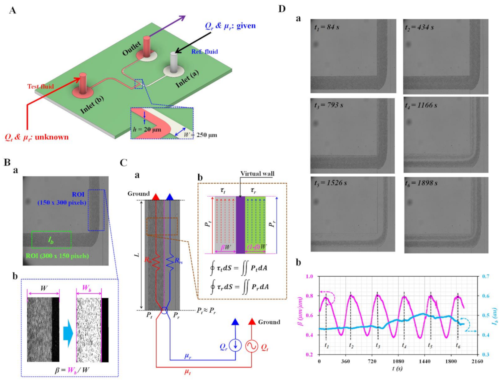
As shown in Figure 1A, the microfluidic device consisted of two guiding microchannels for two fluids (width [W] = 250 µm), a coflowing channel (W = 250 µm), two inlets (a, b), and one outlet. The depth (h) of all channels is set to h = 20 μm. A polydimethylsiloxane (PDMS) block was replicated from a silicon master mold using microfabrication procedures, such as photolithography and soft lithography [52].

Two inlets and one outlet of the PDMS block were punched with a biopsy punch (outer diameter = 0.75 mm). Using an oxygen plasma system, a microfluidic device was fabricated by bonding the PDMS block onto a glass substrate. The microfluidic device was positioned on an inverted microscope (IX53, Olympus, Tokyo, Japan) with a 4× objective lens (NA = 0.1). The ends of two polyethylene tubing (inner diameter = 250 µm, length = 300 mm) were connected to each inlet (a, b). The end of the polyethylene tubing (inner diameter = 250 µm, length = 200 mm) was tightly fitted to the outlet. To remove air from the microfluidic channels and avoid the non-specific binding of plasma proteins inside microfluidic channels, 2 mg/mL bovine serum albumin solution was supplied through the outlet. After 10 min, the microfluidic channels were filled with 1× PBS (pH 7.4, Gibco, Life Technologies, Carlsbad, CA, USA). Two disposable syringes (~1 mL) were filled with glycerin 20% (reference fluid) and blood (test fluid). Each needle of the syringe was fitted to the open end of the individual tubing inserted into the inlet. Two syringes were then installed in a syringe pump (neMESYS, Cetoni Gmbh, Korbussen, Germany). The syringe pump was set to the flow rate of the test fluid (Q_t) for supplying blood in a constant or sinusoidal pattern. The viscosity of the test fluid (µ_t) is not specified. The flow rate of the reference fluid remained unchanged over time (Q_r). Viscosity of glycerin solution (20%) was given as µ_r = 1.93 ± 0.05 cP [53].

A high-speed camera (FASTCAM MINI, Photron, Tokyo, Japan) was used to capture microscopic images of blood flowing in the microfluidic channels. The frame rate of the camera was set to 5000 frames per second. Microscopic images were captured sequentially at intervals of 1 s. All experiments were conducted at a constant temperature of 25 °C.

2.2. Quantification of Image Intensity and Interfacial Location in Coflowing Channel

As shown in Figure 1B(a), two regions of interest (ROIs) were selected to obtain the intensity of the blood image (I_b) and interface (β) between the two fluids using commercial software (MATLAB 2021a, MathWorks, Natick, MA, USA). To monitor RBC volume within blood flows (i.e., hematocrit), the intensity of the blood image was obtained by analyzing the blood image selected inside the guiding channel filled with blood. A specific ROI of the guiding channel of the test fluid was set to 300 × 150 pixels. The intensity (I_b) was then obtained by averaging the grayscale intensity distributed over the ROI. To obtain the interfacial location between the two fluids, a specific ROI was set to 150 × 300 pixels along the coflowing channel. As shown in Figure 1B(b), the grayscale image was converted into a binary image using Otsu’s method [54]. The blood-filled width (W_b) was obtained by averaging the interface distributed over the ROI. The interface (β) was calculated as β = W_b/W.

2.3. Mathematical Representation of Pressure and Shear Stress of Each Stream in Coflowing Channel

To determine analytical expressions of pressure and shear stress, the coflowing channel filled with the test fluid and reference fluid was analytically modeled with discrete fluidic circuit elements (i.e., flow rate and fluidic resistances). As shown in Figure 1C(a), the coflowing channel consists of two streams (i.e., reference fluid stream [r] and test fluid stream [t]). Each stream was represented mathematically by fluidic discrete elements, such as fluidic resistance (R_t, R_r) and fluid rate (Q_r, Q_t). “Ground” indicated zero pressure as the reference value. As the coflowing channel (channel length [L]) had a straight and rectangular channel, both streams had the same pressure (i.e., P_t ≈ P_r). Although the analytical expression of pressure was reported in a previous study [55], the measurement accuracy deteriorated significantly when the interface moved to each wall from the middle plane [56]. Instead of the previous analytical model, a simple discrete circuit model was suggested using the virtual wall concept. As shown in Figure 1C(b), each stream was separated mathematically using a virtual wall. The coflowing channel was partially filled with the test fluid stream (β × W) and the reference fluid stream ([1 − β] × W). According to a previous study [30], a correction factor for pressure (C_P) was included to compensate for the difference in boundary conditions between the real physical model and discrete circuit model. For a rectangular channel with a lower aspect ratio of 0.08 [57], the analytical expression of the pressure for each fluid stream was derived as

$$P_t=\frac{12 {\mu }_{t}L}{C_P \beta W h^3}\times Q_t, \mathrm{for} \mathrm{the} \mathrm{test} \mathrm{fluid} \mathrm{stream}$$

(1)

$$P_r=\frac{12 {\mu }_{r}L}{\left(1-\beta \right) W h^3}\times Q_r \mathrm{for} \mathrm{the} \mathrm{reference} \mathrm{fluid} \mathrm{stream},$$

(2)

respectively. Here, µ_r and µ_t are the viscosities of the reference and test fluids, respectively. Using the same pressure condition (P_t = P_r), the viscosity of the test fluid was derived as follows:

$${\mu }_t={\mu }_r\times \frac{\beta }{1-\beta }\times C_P\times \left(\frac{Q_r}{Q_t}\right)$$

(3)

Based on the force balance between the shear stress and pressure along the test fluid stream (i.e., $\oint {\tau }_{r}dS=\iint P_{r}dA$), the relationship between shear stress and pressure was given as ${\tau }_r\times \left(2\beta W\times L\right)=P_r\times \left(\beta W\times h\right)$. Here, it was assumed that the shear stress acted along the top and bottom surfaces. Using Equation (1), the shear stress of the reference fluid stream (τ_r) was calculated as:

$${\tau }_r={\mu }_r\times \frac{6Q_r}{\left(1-\beta \right)\times W\times h^2}$$

(4)

Using a procedure similar to that discussed as above, the shear stress of the test fluid stream was derived as follows:

$${\tau }_t={\mu }_t\times \frac{6Q_t}{C_P\times \beta \times W\times h^2}$$

(5)

From Equations (3)–(5), both streams in the coflowing channel had the same shear stress (i.e., τ_r = τ_t).

2.4. Quantification of Interface (β) and Intensity (I_b) as Preliminary Study

To demonstrate the relevance of the present method, blood (Hct = 30%) was prepared as the test fluid by adding normal RBCs into autologous plasma, which showed a high degree of RBC sedimentation in the driving syringe [42]. The driving syringe was aligned in the horizontal direction, as shown in the inset of Figure 7A(b). Glycerin solution (20%) was selected as the reference fluid to obtain a distinctive interface. Using syringe pumps, flow rates of the reference fluid and test fluid set to Q_r = 0.5 mL/h and Q_t = 0.7 + 0.5 sin (2 π t/360) mL/h, respectively. Figure 1D(a) showed microscopic images captured over time (t = 84, 434, 793, 1166, 1526, and 1898 s). Based on the quantification methods, temporal variations in β and I_b were obtained over time. RBC sedimentation in the driving syringe caused a decrease in RBCs during blood flow. The hematocrit of blood decreased significantly after t = t₃. However, it tended to decrease after t = t₆. According to previous experimental results obtained with the micro-PIV technique [41], hematocrit had a strong influence on blood velocity obtained with micro-PIV. In this study, it was impossible to obtain information on the hematocrit of blood flow over time. Furthermore, blood flow did not exhibit a uniform distribution of RBCs across the microchannels. Thus, the micro-PIV technique was not considered as effective for monitoring blood flow. On the other hand, the interface between the two fluids was clearly shown in the coflowing channel. According to the present method, the pressure or shear stress of blood flows could be used for monitoring blood flows, even without any issues. Thus, instead of the micro-PIV technique, the present method could be considered a promising tool for monitoring blood flow over time.

2.5. Suspended Blood Preparation Procedure

This study was approved by the ethics committee of Chosun University under the reference code IRB-2-1041055-AB-N-01-2021-05. Concentrated RBCs were purchased from the Gwangju–Chonnam blood bank (Gwangju, Korea) and stored in a refrigerator at 4 °C. Whenever a specific blood sample was required to conduct experiments, normal RBCs and autologous plasma were obtained by removing the buffy layer and debris using the washing procedures reported in our previous study [52]. Subsequently, suspended blood was prepared by adding normal RBCs to a specific diluent (i.e., 1× PBS, plasma, glycerin solution, and dextran solution). First, to evaluate the contributions of hematocrit, the hematocrit of blood was adjusted to Hct = 0, 20%, 30%, 40%, and 50% by adding normal RBCs into 1× PBS or plasma. Second, to stimulate RBC aggregation in the control blood, several concentrations of dextran solutions ranging from 0 to 30 mg/mL at intervals of 10 mg/mL were diluted by dissolving dextran powder (Leuconostoc spp., MW = 450–650 kDa, Sigma–Aldrich, St. Louis, MO, USA) in 1× PBS. Aggregation-enhanced blood was then prepared by suspending normal RBCs in dextran solutions of different concentrations.

3. Results and Discussion

3.1. CFD Simulation for Validation of Analytical Expressions

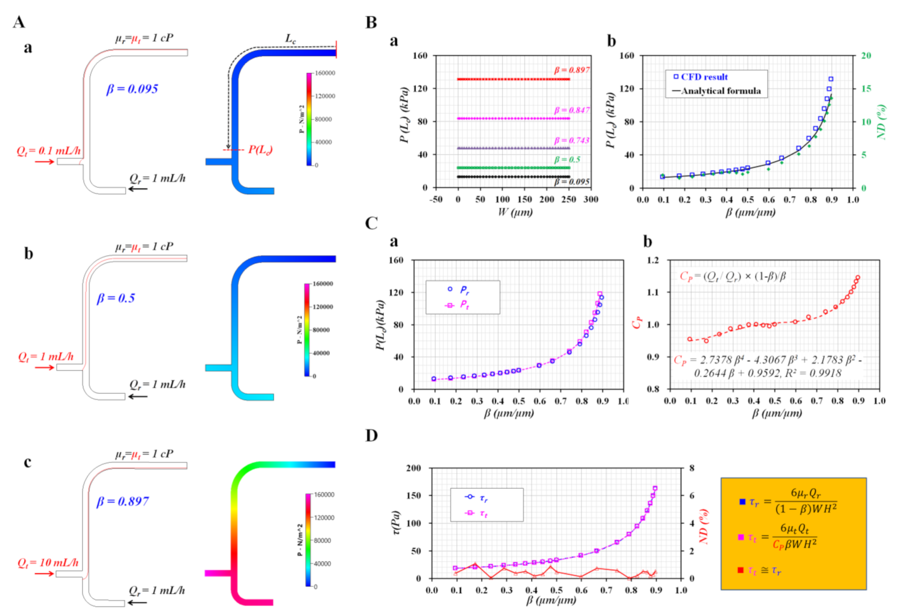
To obtain the correction factor of pressure (C_P) which compensates for the approximation errors that occurred for modeling coflowing lamina streams, computational fluid dynamics (CFD) simulations were conducted using commercial software (CFD-ACE+, Ver. 2019, ESI Group, Paris, France). Using a two-phase module, variations of interfacial locations were estimated by the varying flow rate ratios of two fluids. It was assumed that both fluids behaved as Newtonian fluids. For convenience, both fluids had the same viscosity (µ_r = µ_t = 1 cP). The pressure and interface obtained with the CFD simulation were used to obtain the C_P with respect to the interface. To relocate the interface in the coflowing channel, the flow rate of the test fluid increased from Q_t = 0.1 mL/h to Q_t = 10 mL/h. Here, the flow rate of the reference fluid was fixed at Q_r = 1 mL/h. As shown on the left side panel of Figure 2A, the interfaces (i.e., solid line with red color) were represented with respect to Q_t (i.e., [a] β = 0.095 for Q_t = 0.1 mL/h, [b] β = 0.5 for Q_t = 1 mL/h, and [c] β = 0.897 for Q_t = 10 mL/h).

The right-hand panel of Figure 2A showed the distribution of pressure along the coflowing channel with respect to Q_t. According to the simulation results, β and the pressure increased considerably at higher flow rates of the test fluid. Figure 2B showed a quantitative comparison of the pressure between the CFD simulation and analytical formula (Equations (1) and (2)). As the pressure was proportional to the channel length (L), for convenience, the pressure distribution was obtained at L_c = 7 mm from the ground (i.e., P[L_c]). As shown in Figure 2B(a), variations in pressure across the channel width (W) were obtained with respect to β = 0.095, 0.5, 0.743, 0.847, and 0.897. The pressure (P[L_c]) remained unchanged along the channel width. It tended to increase substantially with increasing β. Figure 2B(b) showed the variations in pressures obtained with both methods (i.e., CFD simulation and analytical method: Equation (2)) with respect to β. In addition, the normalized difference (ND) between the two methods was obtained with respect to β. The CFD simulation overestimated the pressure slightly compared with the analytical formula. When β relocated from 0.1 to 0.9, pressure increased significantly from 13.14 kPa to 131.38 kPa. The ND increased from 2% to 13.6%. As shown in Figure 2C(a), variations in P_r and P_t were obtained with respect to β. As a principle, both streams should have the same pressure in a straight coflowing channel (i.e., P_r = P_t). Here, the pressure of the test fluid stream (P_t) was calculated with respect to β after removing the C_P in Equation (1). However, the difference between P_r and P_t tended to increase when the interface shifted toward the right-side wall.

To minimize the difference between P_r and P_t with respect to β, it was necessary to include C_P in Equation (1). Based on the viscosity formula derived at the same pressure condition (i.e., Equation (3)), C_P was obtained as C_P = (Q_t/Q_r) × (1 − β)/β with respect to β. Figure 2C(b) showed the variations of C_P with respect to β. The C_P tended to increase substantially when the interface moved from the left-side wall to the right-side wall. Linear regression analysis was used to obtain the polynomial expression of C_P as C_P = 2.7378 β⁴ − 4.3067 β³ + 2.1783 β² − 0.2644 β + 0.9592 (R² = 0.9918). When the interface was positioned between β = 0.3, and β = 0.7, both streams had the same pressure within 1% ND, even without including C_P. As shown in Figure 2B(b), the ND between the analytical formula and CFD simulation was less than 6%. Two Equations (1) and (2) were then used to consistently estimate the pressure of each stream in the coflowing channel.

Next, it was necessary to validate the shear stress relationship of each stream in the coflowing channel (i.e., Equations (3) and (4)). Figure 2D showed the variations in τ_r and τ_t with respect to β. The ND between τ_r and τ_t was obtained with respect to β.

As the ND was less than 1% when β was relocated from 0.1 to 0.9, the results indicated that both streams had the same shear stress (τ_r = τ_t). Both shear stresses increased at higher interface values. Furthermore, the shear stress of each stream exhibited remarkably similar variations with respect to β when compared with the pressure of each stream. Based on the pressure correction factor obtained from the CFD simulation results, it was validated that both streams in the coflowing channel had the same pressure and shear stress. The analytical expression of the shear stress and pressure could be used to monitor the test fluid (i.e., pure liquid or blood) flowing in the microchannel.

3.2. Various Flow Rate Patterns of Pure Liquid Controlled with Syringe Pump

Before testing the blood with the present method, glycerin solutions (glycerin = 10%, 20%, and 30%) were used as the test fluid for validating the present method. 1× PBS was selected as the reference fluid for clearly visualizing the interface between both fluids in the coflowing channel. Here, a syringe pump was applied to control the flow rate of the test fluid in two different patterns, including a constant flow rate and a sinusoidal flow rate with different periods.

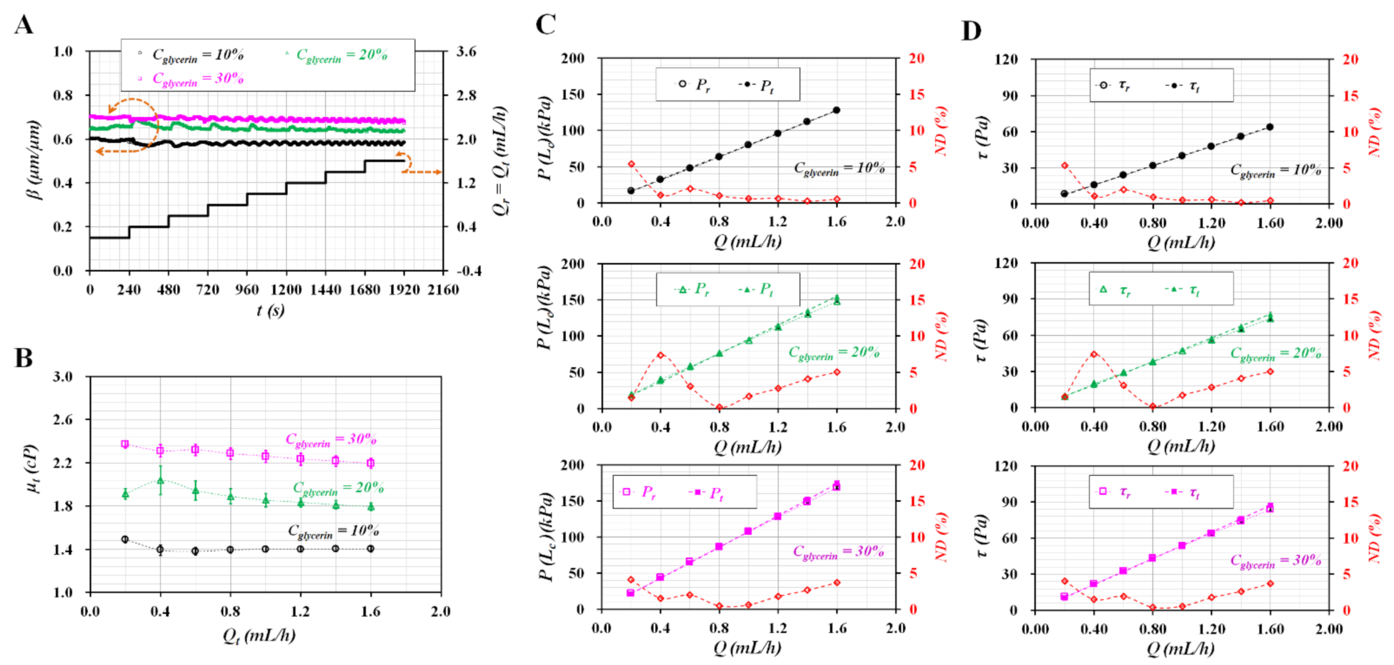
First, while the flow rate of each fluid increased stepwise from 0.2 mL/h to 1.6 mL/h at intervals of 0.2 mL/h, both fluids were supplied into the microfluidic device at the same flow rate (Q_r = Q_t). The variations in pressure and shear stress were obtained by increasing the flow rate of the test fluid. Figure 3A showed the temporal variation of β as well as the flow rate (Q_r or Q_t) with respect to glycerin. The results showed that β tended to increase at higher concentrations of the glycerin solution. Above 0.4 mL/h, it remained unchanged with respect to Q_t. Using Equation (3), the viscosity of each concentration of the glycerin solution was obtained with respect to the flow rate (Q_t). Figure 3B showed the variations in the viscosity of the glycerin solution with respect to Q_t. At lower flow rates (i.e., Q_t ≤ 0.4 mL/h), the viscosity of the glycerin solution exhibited fluctuations with respect to Q_t because the syringe pump induced unstable fluid flows at sufficiently low pressure (i.e., low flow rate or low fluidic viscosity) [58,59]. However, at higher flow rates (i.e., Q_t > 0.4 mL/h), the viscosity remained constant with respect to Q_t. The results indicated that the glycerin solution behaved as a Newtonian fluid. The viscosity of the test fluid was represented as the mean ± standard deviation from several viscosities obtained for each fluid rate. The corresponding viscosity of each glycerin solution was obtained as (a) µ_t = 1.408 ± 0.033 cP for C_glycerin = 10%, (b) µ_t = 1.885 ± 0.08 cP for C_glycerin = 20%, and (c) µ_t = 2.274 ± 0.059 cP for C_glycerin = 30%. When compared with the reference viscosity reported in a previous study [53], linear regression analysis yielded a higher value of correlation (R² = 0.94). In addition, the present method underestimated the values slightly. Based on the quantitative comparison, the viscosity of the test fluid obtained with the present method was used to evaluate the shear stress of the test fluid stream using Equation (5). As shown in Figure 3C, variations in P_r and P_t were obtained with respect to Q_t and C_glycerin. Variations in ND were also summarized with respect to Q_t as well as glycerin. From the results, the pressure of both streams (P_r, P_t) increased linearly with respect to Q_t. Above Q_t = 0.4 mL/h, the ND was less than 5%. Both streams had approximately the same pressure. P_t required two vital factors (i.e., flow rate, and viscosity) in advance. As P_r could be evaluated by measuring β, the pressure of the test fluid stream could be quantified by measuring P_r indirectly. Figure 3D showed the variations in τ_r and τ_t with respect to Q_t and C_glycerin. Variations in ND were also obtained with respect to Q_t and glycerin. Similar to the variations in pressure (P_r, P_t), both the shear stresses (τ_r, τ_t) increased linearly with respect to Q_t. The ND was less than 5% above Q_t = 0.4 mL/h. Thus, the shear stress of the test fluid stream (τ_t) could be obtained indirectly by measuring τ_r.

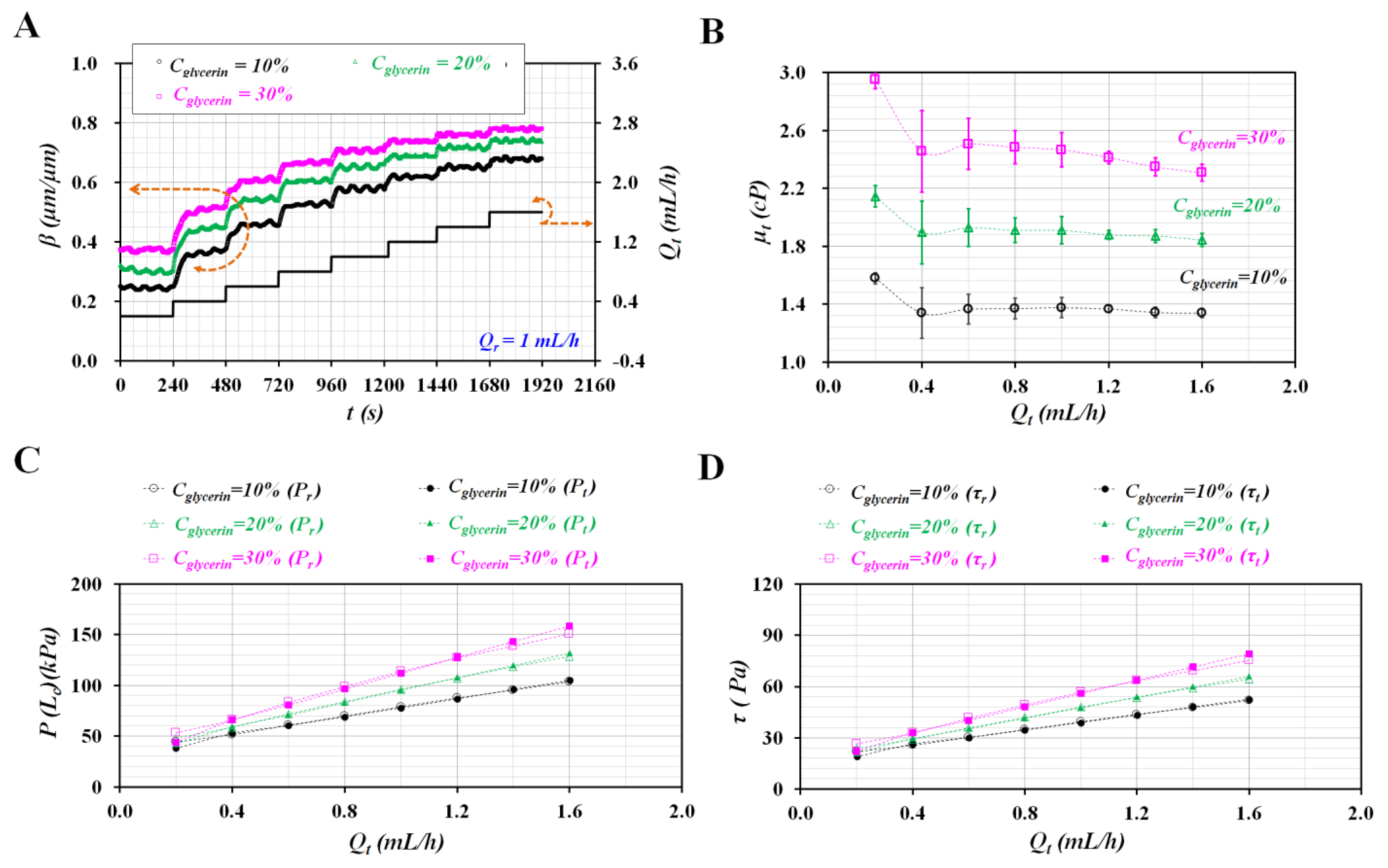
Second, 1× PBS was supplied to the microfluidic device at a constant flow rate of 1 mL/h (Q_r = 1 mL/h). The flow rate of the test fluid increased stepwise from 0.2 mL/h to 1.6 mL/h at intervals of 0.2 mL/h. As shown in Figure 4A, the temporal variations in β were obtained with respect to glycerin and Q_t. The value of β increased gradually at higher flow rates and higher concentrations of the glycerin solution. The viscosity of the glycerin solution was then calculated by substituting β and Q_t into Equation (3). Figure 4B showed the viscosity of the glycerin solution with respect to Q_t as well as C_glycerin. Above Q_t = 0.4 mL/h, the viscosity of the test fluid remained constant with respect to Q_t. The corresponding viscosity of each glycerin solution was obtained as (a) µ_t = 1.357 ± 0.016 cP for C_glycerin = 10%, (b) µ_t = 1.891 ± 0.029 cP for glycerin = 20%, and (c) µ_t = 2.425 ± 0.074 cP for glycerin = 30%. When compared with the viscosities obtained under the same flow rate condition (Q_r = Q_t), the viscosity of the test fluid showed substantially similar values with respect to C_glycerin. To determine the correlation of viscosities obtained under two different flow rate conditions, a linear regression analysis was conducted using experimental data as shown in Figure 3B and Figure 4B. As a result, the linear regression was obtained as µ (Q_r ≠ Q_t) = 1.026 × µ (Q_r = Q_t) (R² = 0.9685). From the quantitative study, the present method quantified the viscosity of the test fluid consistently, without respect to flow rate condition (i.e., Q_r = Q_t, Q_r ≠ Q_t). Figure 4C showed the variations of P_r and P_t with respect to glycerin concentration and Q_t. Both pressures tended to increase linearly with respect to Q_t. In addition, there was little difference between P_r and P_t (P_r ≈ P_t). Figure 4D showed the variations in τ_r and τ_t with respect to glycerin concentration and Q_t. Both shear stresses tended to increase linearly with respect to Q_t. Namely, higher concentrations of glycerin solution resulted in higher shear stress values. Furthermore, there was little difference between τ_r and τ_t with respect to Q_t. On the other hand, when compared with the pressure and shear stress as shown in Figure 3C,D, the shear stress and pressure which are represented in Figure 4C,D decreased substantially because the flow rate of the reference fluid remained constant at 1 mL/h.

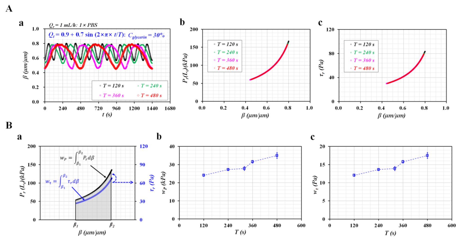
Third, to induce a sinusoidal flow in the test fluid, glycerin solution (C_glycerin = 30%) as test fluid was supplied at a flow rate of Q_t = 0.9 + 0.7 sin (2 × π × t/T) mL/h. Here, the period (T) set to T = 120, 240, 360, and 480 s. The reference fluid was supplied at a constant flow rate of 1 mL/h. Variations in the pressure and shear stress (i.e., P_r and τ_r) were obtained with respect to T. Here, it was impossible to obtain the flow rate (Q_t) and viscosity (µ_t) of the test fluid in advance. In the coflowing channel, it was already validated that both streams had the same pressure and shear stress (i.e., P_r ≈ P_t, τ_r ≈ τ_t). Both properties of the test fluid could be then obtained indirectly by quantifying the pressure (P_r) and shear stress (τ_r) of the reference fluid because three vital properties (i.e., µ_r, Q_r, and 1 − β) of the reference fluid were obtained over time.

Figure 5A(a) showed the temporal variations of β with respect to T. As T increased, the maximum value of β remained unchanged with respect to T. The minimum value of β decreased substantially when T increased from T = 120 s to T = 360 s. The minimum value of β did not show a difference between T = 360 s and T= 480 s. Based on temporal variations in β over time as shown in Figure 5A(a), variations in P_r (L_c) were obtained with respect to T and β. As shown in Figure 5A(b), P_r tended to increase gradually with respect to β. Four trajectories (i.e., P_r vs. β) overlapped well with respect to T. The minimum values of P_r and β tended to decrease with decreasing T. Figure 5A(c) showed the variations in τ_r with respect to T and β. τ_r showed remarkably similar behaviors to P_r with respect to T. According to Equations (2) and (4), P_r and τ_r were proportional to (1 − β)⁻¹. From Figure 5A(b,c), it was impossible to determine the relationship between P_r and β with respect to T. To quantify the contribution of T to P_r or τ_r, the other parameter (i.e., work = pressure × volume or shear stress × volume) was proposed by analyzing P_r or τ_r with respect to β for each period. As shown in Figure 5B(a), to construct the X-Y plot, P_r (or τ_r) and β were graphically represented on the Y-axis and X-axis, respectively. According to the definition of work, the pressure-volume work (W_P) was calculated as W_P $={{\displaystyle \int }}_{V_1}^{V_2}{P}_{r}dV$. The infinitesimal volume (dV) becomes dV = L × h × (W dβ) as shown in Figure 1C. The W_P was then calculated as W_P = $V\times {{\displaystyle \int }}_{{\beta }_1}^{{\beta }_2}{P}_{r}d\beta$. As the volume of the coflowing channel (V = L × h × W) remained constant, the pressure unit volume work (i.e., w_p = W_P/V) was then calculated as w_p $={{\displaystyle \int }}_{{\beta }_1}^{{\beta }_2}{P}_{r}d\beta$. Here, β₁ and β₂ represent the minimum and maximum values of β obtained for a single period, respectively. Similarly, using the same procedure for calculating w_P as above, the shear stress-volume work (W_t) was derived as W_t = $V\times {{\displaystyle \int }}_{{\beta }_1}^{{\beta }_2}{\tau }_{rs}d\beta$. The shear stress-unit volume work (i.e., w_τ = W_t/V) was calculated as w_τ = ${{\displaystyle \int }}_{{\beta }_1}^{{\beta }_2}{\tau }_{r}d\beta$. As shown in the inset of Figure 5B(a), w_P and w_τ are represented graphically by means of an X-Y plot (i.e., P_r vs. β, τ_r vs. β). Figure 5B(b,c) showed variations in w_P and w_τ with respect to T. w_P tended to increase with respect to T. As shown in Figure 5A(a), the minimum value of β (i.e., β₁) decreased at higher values of T. Integration of P_r from β₁ to β₂ increased at higher values of T. Similarly, w_τ tended to increase with respect to T. The variations in w_τ were remarkably similar to w_P with increasing T.

From the experimental results, the present method was effectively applied to monitor the flow of glycerin solution as a test fluid under constant flow rates as well as sinusoidal flow rates. As both streams in the coflowing channel had the same pressure and shear stress (i.e., P_r ≈ P_t, τ_r ≈ τ_t), the pressure and shear stress of the test fluid were estimated in terms of the pressure and shear stress of the reference fluid. Thus, four properties of the test fluid (i.e., P_r, τ_r, w_P, and w_τ) were calculated consistently by monitoring the interface between the two fluids under various flow rate conditions.

3.3. Sinusoidal Flow Rates of Blood Controlled with Syringe Pump

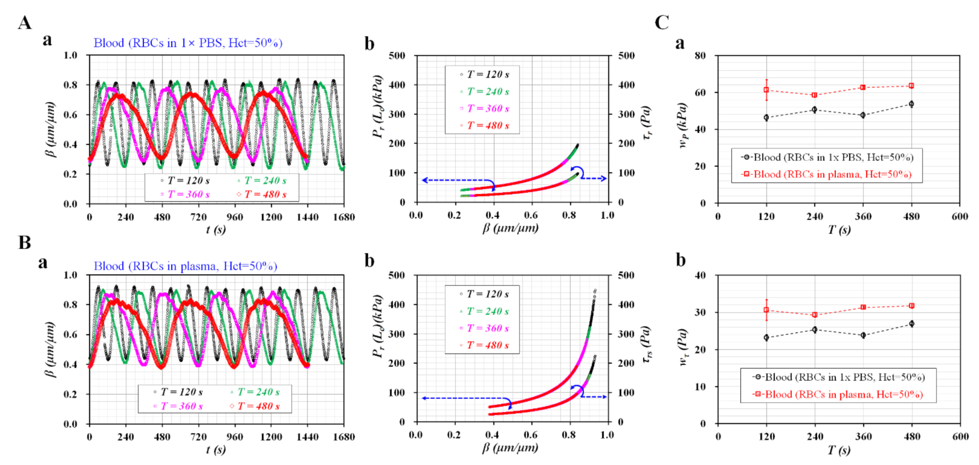
Instead of glycerin solutions as the test fluid, the present method was applied to quantify four properties of blood flows (i.e., pressure, shear stress, pressure unit volume work, and shear stress unit volume work) under sinusoidal flow rates. To clearly detect the interface in the coflowing channel, a glycerin solution (20%) was supplied as a reference fluid. The flow of the reference fluid was set to 0.5 mL/h. Blood (Hct = 50%) as the test fluid was prepared by adding normal RBCs into a diluent (1× PBS, plasma). The blood flow rate set to Q_t = 0.9 + 0.7 sin (2 × π × t/T) mL/h. The period (T) set to T = 120, 240, 360, and 480 s. The contributions of the period to P_r (L_c) and τ_r were evaluated for normal RBCs suspended in 1× PBS and plasma. Figure 6A(a) showed the temporal variations of β with respect to T. When T increased from 120 s to 480 s, the alternating amplitude of β (Δβ) (i.e., Δβ = maximum value of β—minimum value of β) tended to decrease gradually. Figure 6A(b) showed the variations of P_r (L_c) and τ_r with respect to β and T. Four trajectories represented between P_r and β overlapped nearly with respect to T. τ_r showed similar trends to P_r with respect to T. On the other hand, while replacing 1× PBS with plasma as a diluent, contributions of T to P_r (L_c) and τ_r were obtained for normal RBCs suspended in plasma. Figure 6B(a) showed the temporal variations of β with respect to T. When compared with 1× PBS as diluent, plasma as diluent contributed substantially to increasing β. The Δβ tended to decrease at higher values of T. Figure 6B(b) showed variations in P_r (L_c) and τ_r with respect to β and T. When compared with Figure 6A(b), the pressure (P_r) and shear stress (τ_r) increased substantially. However, P_r and τ_r did not show substantial differences in trajectories (i.e., P_r vs. β, τ_r vs. β). Furthermore, two works (w_P, w_τ) were obtained by analyzing P_r and τ_r with respect to β. Figure 6C(a) showed variations in w_P with respect to T and diluent (1× PBS, plasma). Plasma as a diluent caused a significant increase in w_P when compared with 1× PBS as a diluent. Additionally, w_P increased potentially with respect to T. Figure 6C(b) showed variations of w_τ with respect to T and diluent. The variation of w_τ was like that of w_P with respect to T and the diluent. From the experimental results, the difference in the diluent (i.e., 1× PBS, plasma) could be detected by calculating w_P or w_τ. T had a considerable influence on w_P and w_τ. Thus, it was necessary to fix the period of sinusoidal blood flow to effectively evaluate the difference in blood flow using w_P or w_τ.

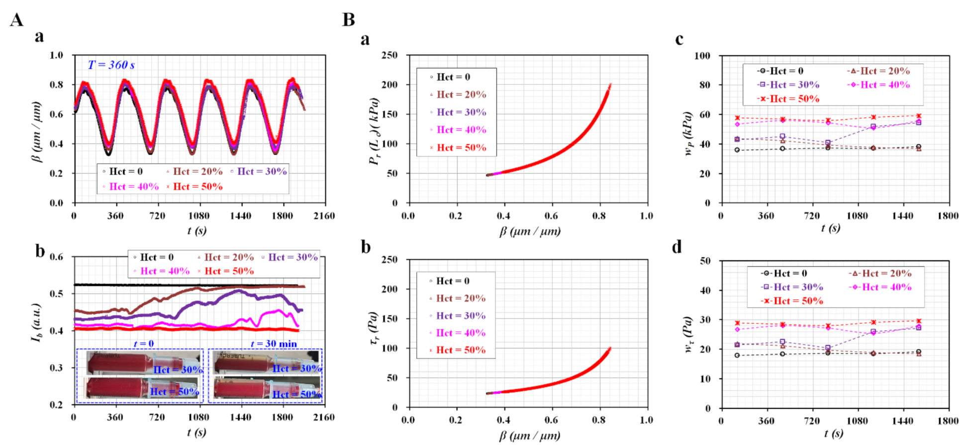
As the hematocrit of blood had a strong influence on blood flow, the four properties of blood flow (i.e., P_r, τ_r, w_P, and w_τ) were obtained by setting Hct = 0, 20%, 30%, 40%, and 50%. Hct = 0 indicates no RBC inclusion. Each hematocrit value was adjusted by adding normal RBCs into the plasma. A driving syringe filled with blood was installed horizontally, as shown in the inset of Figure 7A(b). The period (T) of the sinusoidal blood flow was fixed at T = 360 s. As shown in Figure 7A(a), temporal variations in β were obtained with respect to Hct. β tends to increase significantly with increasing hematocrit. Figure 7A(b) showed the temporal variations of I_b with respect to Hct. The inset of Figure 7A(b) showed snapshots of a driving syringe filled with blood (Hct = 30%, and 50%) captured at t = 0 and t = 30 min. At lower hematocrit levels ranging from 20% to 40%, the I_b increased significantly over time. Due to RBC sedimentation in the driving syringe, the hematocrit of blood flowing in the guide channel for blood decreased substantially after a certain time. A decrease in hematocrit caused an increase in the I_b. The time (t_b), when I_b started to increase substantially, tended to increase with increasing hematocrit (i.e., [a] t_b = 480 s for Hct = 20%, [b] t_b = 870 s for Hct = 30%, and [c] t_b = 1560 s for Hct = 40%). However, at the highest level of Hct = 50, the I_b remained constant over time. Figure 7B(a,b) showed variations in P_r (L_c) and τ_r with respect to Hct and β. P_r and τ_r tended to increase at higher hematocrit levels. In addition, β tended to increase with increasing hematocrit levels. Based on the variations of P_r and τ_r with respect to β, temporal variations in w_P and w_τ were obtained with respect to Hct. Figure 7B(c) showed the temporal variations of w_P with respect to Hct. Plasma (Hct = 0) did not contribute to the variation in w_P over time. For blood with Hct = 20%, w_P decreased gradually over time. Blood with Hct = 30% exhibited an increase in w_P after t = 720 s. The higher hematocrit level (Hct = 40–50%) did not significantly contribute to varying w_P over time. The w_P tended to increase with increasing Hct. Figure 7B(d) showed the temporal variations of w_τ with respect to Hct. The variation in w_τ was remarkably like that of w_P with respect to Hct. Above Hct = 40%, w_τ remained constant over time. Thus, either w_P or w_τ could be used to monitor the hematocrit in blood flow.

From the experimental results, the present method can evaluate blood flows with sinusoidal patterns controlled by a syringe pump. As our properties of blood flow (i.e., P_r, τ_r, w_P, and w_τ) were influenced by period (T), it was necessary to maintain a constant period during the experiment. They were used effectively to evaluate variations in hematocrit in blood flow.

3.4. Blood Flows Controlled with Peristaltic Pump

To supply the blood with a peristaltic flow pattern, the syringe pump was replaced by a peristaltic pump. Quantitative information on blood flow controlled by the peristaltic pump was not specified. Based on a flow stabilizer [58], unstable blood flow was stabilized with an air compliance effect. By adjusting the air cavity secured inside the flow stabilizer, variations in the four properties of blood flow (i.e., P_r [L_c], τ_r, w_P, and w_τ) were evaluated. Thereafter, by supplying aggregation-enhanced blood into a microfluidic channel, the four properties were obtained over time.

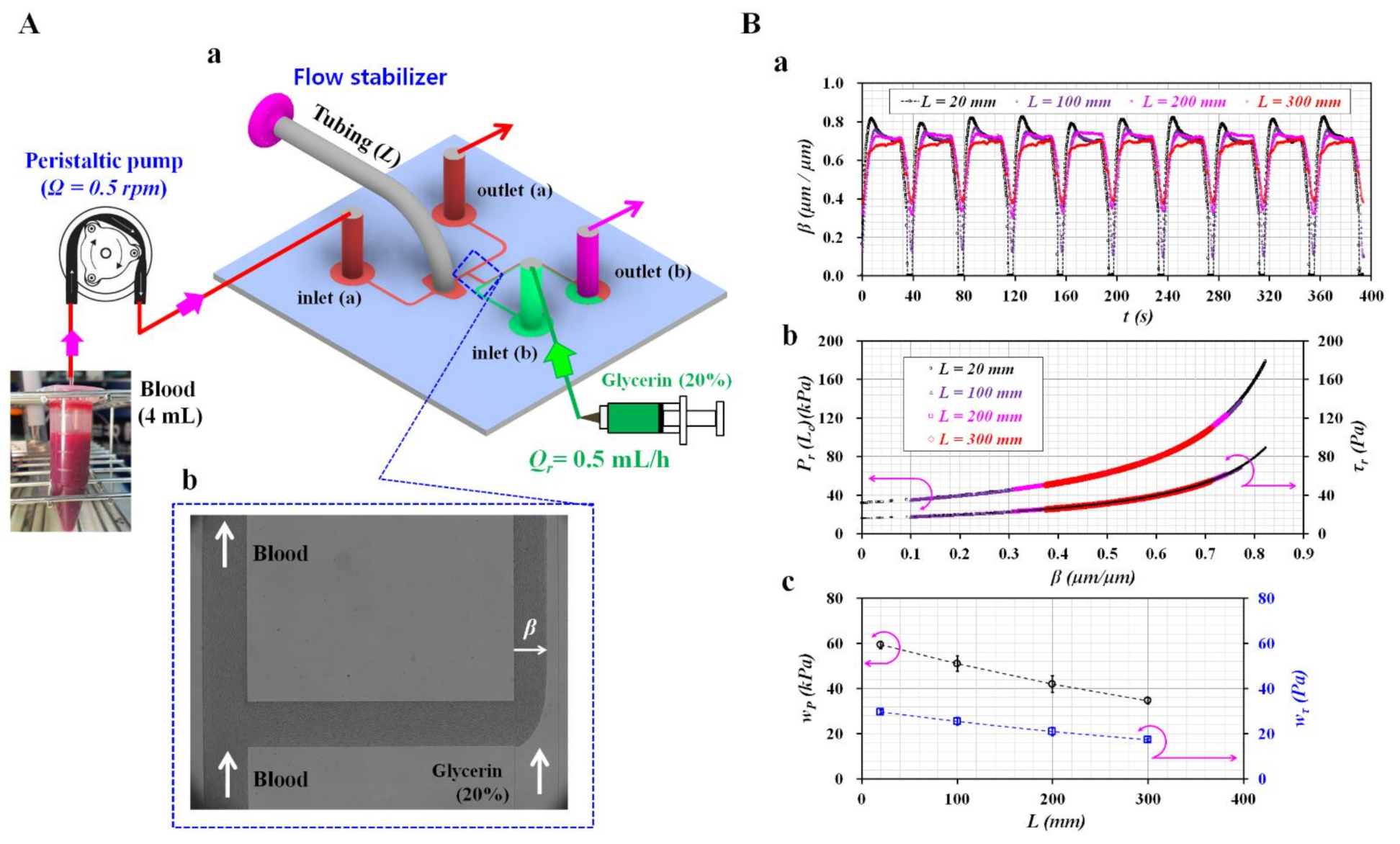
Figure 8A(a) showed a schematic diagram of the in vitro fluidic system. The experimental setup was composed of a microfluidic device integrated with a flow stabilizer, a peristaltic pump (Techpre pump, Jeniwell, Seoul, Korea) for blood, and a syringe pump for glycerin solution (20%). The microfluidic device consisted of two inlets (a, b), two outlets (a, b), two guide channels for two fluids, a coflowing channel, and a large channel for connecting the flow stabilizer. To stabilize unstable pulsatile blood flow by means of the air compliance effect, the air cavity inside the fluidic stabilizer was secured by adjusting the tubing length (L) (L = 20, 100, 200, and 300 mm), and closing one side end with a drawing pin. A tube (~5 mL) was filled with blood (i.e., normal RBCs in plasma, Hct = 50%, and blood volume = 4 mL). A peristaltic pump set to Ω = 0.5 rpm. The syringe pump set to 0.5 mL/h to supply the glycerin solution (20%). Figure 8A(b) showed a microscopic image of microfluidic channels filled with the blood as well as glycerin solution (20%). As blood flow had a higher pressure than the glycerin solution, blood moved from the inlet (a) to the outlet (a). In addition, blood flowed from the connecting channel to the upper right channel (i.e., the coflowing channel). The glycerin solution flowed from the right lower channel to the right upper channel. Blood and glycerin solutions met in the right upper channel (i.e., coflowing channel). The interface (β) was determined by the dynamic flow of the two fluids. Using the present method, it was possible to monitor blood flow in the coflowing channel by means of four blood flow properties (i.e., P_r, τ_r, w_P, and w_τ).

As shown in Figure 8B, the contributions of the flow stabilizer to flow stabilization were quantified by adjusting the length of the tubing size (L). Figure 8B(a) showed the temporal variations of β with respect to L. According to a previous study [58], an air cavity secured inside a disposable syringe caused a substantial increase in air compliance. Without the flow stabilizer, blood did not enter the coflowing channel for a certain duration (i.e., β = 0). Blood flow exhibited peristaltic instability over time. To invade blood into the right upper channel (i.e., coflowing channel) continuously, it was necessary to minimize unstable blood flow by adjusting L. By installing a flow stabilizer into the microfluidic device, blood was filled in the coflowing channels and flowed continuously over time. At L = 20 mm, blood did not invade the right upper channel for a certain duration. When L was increased from 100 mm to 300 mm, the alternating amplitude of β (i.e., the maximum value of β—minimum value of β) tended to decrease over time. As air compliance increased substantially with respect to L, it contributed to stabilizing the unstable blood flow considerably. Figure 8B(b) showed variations in P_r (L_c) and τ_r with respect to β and L. When L was increased from 20 mm to 300 mm, the variation range of P_r and τ_r decreased significantly. The variation range of β also tended to decrease with respect to L. Figure 8B(c) showed variations of w_P and w_τ with respect to L. As the area enclosed between P_r (or τ_r) and β decreased with increasing L, as shown in Figure 8B(b), w_P and w_τ tended to decrease substantially with respect to L. Two properties related to the work (i.e., w_P, w_τ) tended to decrease owing to the flow stabilizer. Thus, four properties estimated by analyzing blood flow could be considered as quantitative factors for analyzing blood flow. P_r and τ_r exhibited similar trends with respect to L. In addition, w_P and w_τ exhibited similar variations with increasing L. Among the four properties, two properties (i.e., P_r, w_P) could be used to monitor blood flow.

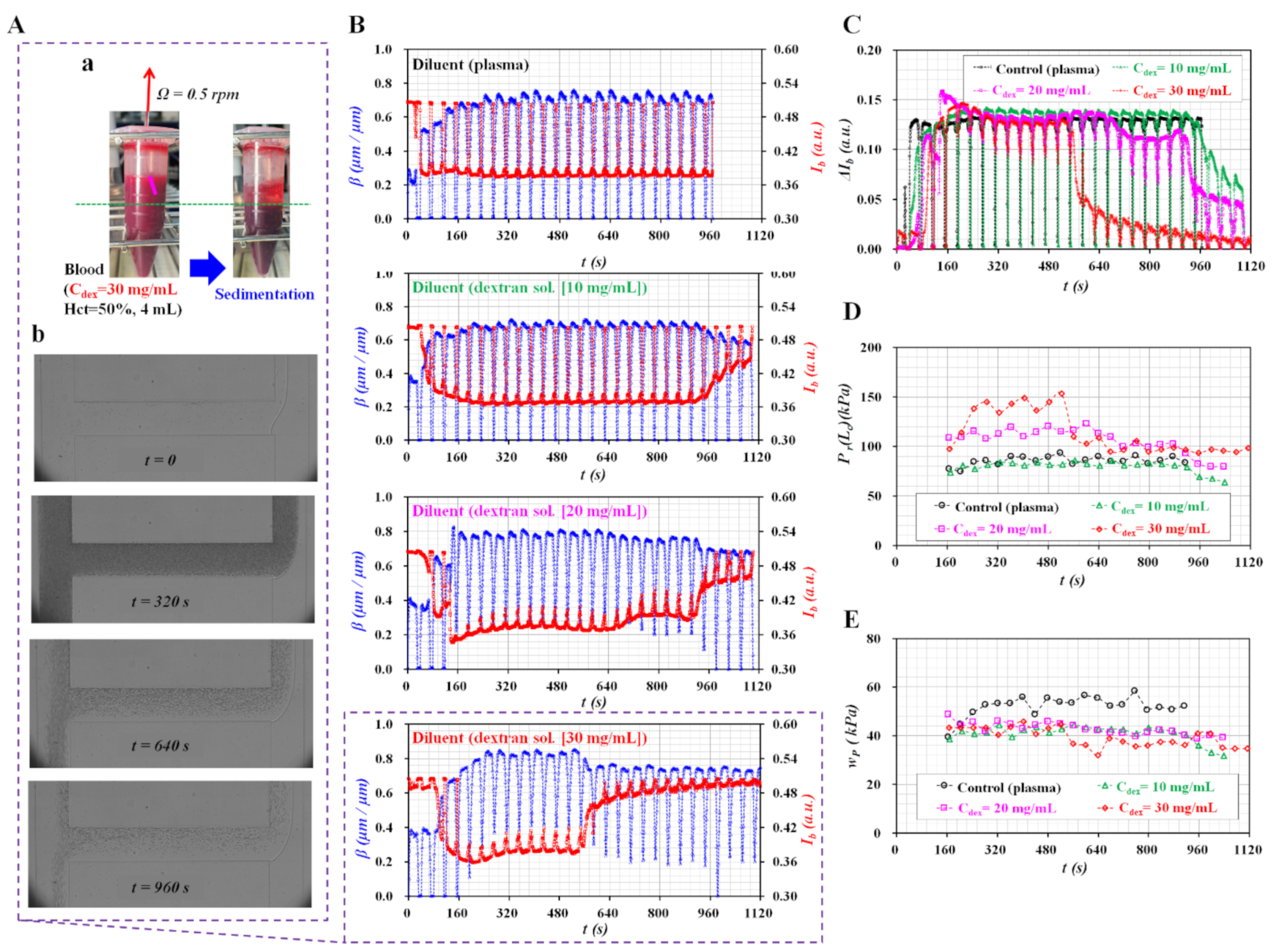
During the demonstration, aggregation-enhanced blood was used to change the hematocrit inside the blood flow. RBC sedimentation in the reservoir caused variations in the hematocrit of blood over time [30]. With respect to the degree of RBC aggregation, the image intensity (I_b) and interface (β) were obtained. Thereafter, two properties of blood flow (P_r, w_P) were obtained by analyzing the temporal variations in β. To enhance RBC aggregation or RBC sedimentation in a tube, aggregation-enhanced blood (Hct = 50%) was prepared by adding normal RBCs into a dextran solution at several concentrations (C_dex = 10, 20, and 30 mg/mL). Control blood (C_dex = 0) was prepared by adding normal RBCs to the plasma. The tube was filled with aggregation-enhanced blood (~4 mL). The tube length (L) of the flow stabilizer was fixed at 200 mm. Figure 9A showed RBC sedimentation in the tube as well as blood flow in microfluidic channels for highly aggregated blood (C_dex = 30 mg/mL). As shown in Figure 9A(a), the dextran solution accelerated RBC sedimentation in the tube. The end of the suction tube was fixed inside the tube. Blood was suctioned through the tube, and RBCs were sedimented continuously. Blood was separated into two layers (i.e., diluent in the upper layer and RBCs in the lower layer) after a certain time.

As shown in Figure 9A(b), microscopic images of blood flow were obtained at specific times (t = 0, 320, 640, and 960 s). Initially (t = 0), blood did not invade the microfluidic channel. At t = 320 s, blood flowed into the microfluidic channel. The right upper channel (i.e., the coflowing channel) was partially filled with a blood and glycerin solution. However, due to RBC sedimentation in the tube, the hematocrit of blood flows (i.e., RBCs distributed in the channel) decreased significantly from t = 640 s to t = 960 s. Figure 9B showed temporal variations in β and I_b with respect to C_dex. The control blood showed consistent variation in I_b and β over time. However, when the concentration of the dextran solution increased from C_dex = 10 mg/mL to C_dex = 30 mg/mL, I_b varied largely over time due to RBC sedimentation in the tube. RBC sedimentation causes a decrease in β over time. In other words, I_b and β varied largely from the specific time when the hematocrit of blood flow began to decrease. Figure 9C showed the temporal variations of ΔI_b with respect to C_dex. ΔI_b was calculated as ΔI_b = I_b (t = 0)—I_b (t). When the hematocrit of blood flow began to decrease, it tended to decrease at higher concentrations of dextran solution. Figure 9D showed the temporal variations of the averaged pressure (P_r [L_c]) calculated for each period with respect to C_dex. Control blood (C_dex = 0) and aggregation-enhanced blood (C_dex = 10 mg/mL) exhibited remarkably similar trends in P_r (L_c) over time. Above C_dex = 10 mg/mL, the dextran solution contributed significantly to increasing P_r (L_c). Furthermore, it tended to decrease gradually after the hematocrit of the blood flow began to decrease. Figure 9E showed the temporal variations of w_P with respect to C_dex. As the pressure-unit volume work (w_P) was calculated using P_r (L_c), w_P exhibited similar variations in P_r. The w_P of the control blood remained constant over time. As shown in Figure 9B, the alternating amplitude of β tended to decrease at higher concentrations of the dextran solution. Thus, aggregation-enhanced blood contributed to decreasing the pressure-unit volume work (w_P) substantially from the specific time when the hematocrit of blood flows began to decrease.

From the demonstration, the present method was used effectively to quantify blood flow when the hematocrit of blood varied continuously over time. For the conventional micro-PIV technique, to obtain consistent velocity fields of blood flow, it is necessary to maintain the uniform distribution of RBCs within blood flows. However, as hematocrit varies greatly over time, it might be difficult to get consistent monitoring of blood flow with the micro-PIV technique. Throughout the demonstration, the present method is better than the micro-PIV technique. As a limitation, the present method was demonstrated using a syringe pump that supplied the reference fluid. To extend the application of the present method, it will be necessary to devise a miniaturized delivery system for supplying the reference fluid at a constant flow rate. The delivery system should be equipped with two vital functions, such as fluid delivery with a micropump [60,61,62] and flow stabilization with a compliance mechanism [58,63,64]. Furthermore, instead of a microscopic image, a laser polarization technique could be used to characterize properties of RBCs (i.e., orientation, osmotic pressure, oxygenation, and equivalent volume) under shear blood flows [65,66]. Shortly, ultimately, the present method might be used for quantifying blood flows in vascularized microfluidic platforms, which contribute to understanding biochemical and biophysical behaviors of micro vasculatures [67,68,69]. Additionally, as blood flow monitoring is considered as one of the key issues in microfluidic platforms, it will be necessary to be integrated into blood-on-a-chip for evaluating physical functions of single cells or separating cells or plasma from patients’ blood [70,71].

4. Conclusions

In this study, a coflowing channel was suggested as a sensorless approach to monitoring blood flow. Information on the blood (i.e., hematocrit, flow rate, and viscosity) was not provided in advance. However, information on the reference fluid (i.e., flow rate, and viscosity) was specified in advance. The dynamic properties of blood flows were then obtained by detecting the interface between two fluids in the coflowing streams. After constructing a discrete circuit model for the coflowing streams, the analytical formulas of pressure and shear stress were derived from the fact that both streams had the same pressure in the straight coflowing channel. Based on CFD simulations, both analytical expressions of pressure and shear stress for each stream were corrected by inserting a pressure correction factor into the expressions. Two types of work related to blood flow (i.e., pressure-unit volume work and shear stress-unit volume work) were derived from the relationship between pressure (or shear stress) and interface. Four properties of blood flow (i.e., pressure, shear stress, and two types of work) were calculated to quantify the flow of the test fluid. In the present method, the four properties were obtained by varying the flow patterns (i.e., constant flow rate or sinusoidal flow rate) or test fluids (i.e., glycerin solutions and blood). The present method was then applied to quantify dynamic flows of aggregation-enhanced blood circulated with a peristaltic pump, where any information regarding the blood was not specified. From the experimental results, the present method has been validated to have the ability to consistently quantify dynamic blood flows, where the hematocrit changed continuously over time.

References

- Popel, A.S.; Johnson, P.C. Microcirculation and hemorheology. Annu. Rev. Fluid Mech. 2005, 37, 43–69. [Google Scholar] [CrossRef] [PubMed] [Green Version]
- Tomaiuolo, G.; Carciati, A.; Caserta, S.; Guido, S. Blood linear viscoelasticity by small amplitude oscillatory flow. Rheol. Acta 2016, 55, 485–495. [Google Scholar] [CrossRef] [Green Version]
- Ahn, C.B.; Kang, Y.J.; Kim, M.G.; Yang, S.; Lim, C.H.; Son, H.S.; Kim, J.S.; Lee, S.Y.; Son, K.H.; Sun, K. The effect of pulsatile versus nonpulsatile blood flow on viscoelasticity and red blood cell aggregation in extracorporeal circulation. Korean J. Thorac. Cardiovasc. Surg. 2016, 49, 145–150. [Google Scholar] [CrossRef]
- Pop, G.A.; Chang, Z.-Y.; Slager, C.J.; Kooij, B.-J.; Deel, E.D.V.; Moraru, L.; Quak, J.; Meijer, G.C.; Duncker, D.J. Catheter-based impedance measurements in the right atrium for continuously monitoring hematocrit and estimating blood viscosity changes; an in vivo feasibility study in swine. Biosens. Bioelectron. 2004, 19, 1685–1693. [Google Scholar] [CrossRef] [PubMed]
- Lima, R.; Ishikawa, T.; Imai, Y.; Takeda, M.; Wada, S.; Yamaguchi, T. Radial dispersion of red blood cells in blood flowing through glass capillaries: The role of hematocrit and geometry. J. Biomech. 2008, 41, 2188–2197. [Google Scholar] [CrossRef] [PubMed] [Green Version]
- Shevkoplyas, S.S.; Yoshida, T.; Gifford, S.C.; Bitensky, M.W. Direct measurement of the impact of impaired erythrocyte deformability on microvascular network perfusion in a microfluidic device. Lab. Chip 2006, 6, 914–920. [Google Scholar] [CrossRef] [PubMed]
- Chien, S. Red cell deformability and its relavance to blood flow. Ann. Rev. Physiol. 1987, 49, 177–192. [Google Scholar] [CrossRef]
- Ermolinskiy, P.; Lugovtsov, A.; Yaya, F.; Lee, K.; Kaestner, L.; Wagner, C.; Priezzhev, A. Eect of red blood cell aging in vivo on their aggregation properties in vitro: Measurements with laser tweezers. Appl. Sci. 2020, 10, 7581. [Google Scholar] [CrossRef]
- Wen, J.; Wan, N.; Bao, H.; Li, J. Quantitative measurement and evaluation of red blood cell aggregation in normal blood based on a modified hanai equation. Sensors 2019, 19, 1095. [Google Scholar] [CrossRef] [Green Version]
- Cho, Y.-I.; Cho, D.J. Hemorheology and Microvascular Disorders. Korean Cir. J. 2011, 41, 287–295. [Google Scholar] [CrossRef] [PubMed] [Green Version]
- Sebastian, B.; Dittrich, P.S. Microfluidics to mimic blood flow in health and disease. Annu. Rev. Fluid Mech. 2018, 50, 483–504. [Google Scholar] [CrossRef]
- Whittaker, S.R.F.; Winton, F.R. The apparent viscosity of blood flowing in the isolated hindlimb of the dog and its variation with corpuscular concentration. J. Physiol. 1933, 78, 339–369. [Google Scholar] [CrossRef] [PubMed] [Green Version]
- Lipowsky, H.H. Microvascular Rheology and Hemodynamics. Microcirculation 2005, 12, 5–15. [Google Scholar] [CrossRef]
- Tomaiuolo, G.; Barra, M.; Preziosi, V.; Cassinese, A.; Rotoli, B.; Guido, S. Microfluidics analysis of red blood cell membrane viscoelasticity. Lab. Chip 2011, 11, 449–454. [Google Scholar] [CrossRef] [PubMed]
- Campo-Deano, L.; Dullens, R.P.A.; Aarts, D.G.A.L.; Pinho, F.T.; Oliveira, M.S.N. Viscoelasticity of blood and viscoelastic blood analogues for use in polydymethylsiloxane in vitro models of the circulatory system. Biomicrofluidics 2013, 7, 034102. [Google Scholar] [CrossRef] [PubMed] [Green Version]
- Kang, Y.J.; Lee, S.-J. Blood viscoelasticity measurement using steady and transient flow controls of blood in a microfluidic analogue of Wheastone-bridge channel. Biomicrofluidics 2013, 7, 054122. [Google Scholar] [CrossRef] [Green Version]
- Kim, M.; Kim, A.; Kim, S.; Yang, S. Improvement of electrical blood hematocrit measurements under various plasma conditions using a novel hematocrit estimation parameter. Biosens. Bioelectron. 2012, 35, 416–420. [Google Scholar] [CrossRef] [PubMed]
- Kim, M.; Yang, S. Improvement of the accuracy of continuous hematocrit measurement under various blood flow conditions. Appl. Phys. Lett. 2014, 104, 153508. [Google Scholar] [CrossRef]
- Lee, H.Y.; Barber, C.; Rogers, J.A.; Minerick, A.R. Electrochemical hematocrit determination in a direct current microfluidic device. Electrophoresis 2015, 36, 978–985. [Google Scholar] [CrossRef]
- Berry, S.B.; Fernandes, S.C.; Rajaratnam, A.; De Chiara, N.S.; Mace, C.R. Measurement of the hematocrit using paper-based microfluidic devices. Lab. Chip 2016, 16, 3689–3694. [Google Scholar] [CrossRef]
- Kim, B.J.; Lee, Y.S.; Zhbanov, A.; Yang, S. A physiometer for simultaneous measurement of whole blood viscosity and its determinants: Hematocrit and red blood cell deformability. Analyst 2019, 144, 3144–3157. [Google Scholar] [CrossRef]
- Jalal, U.M.; Kim, S.C.; Shim, J.S. Histogram analysis for smartphone-based rapid hematocrit determination. Biomed. Opt. Express 2017, 8, 3317–3328. [Google Scholar] [CrossRef] [PubMed] [Green Version]
- Boas, L.V.; Faustino, V.; Lima, R.; Miranda, J.M.; Minas, G.; Fernandes, C.S.V.; Catarino, S.O. Assessment of the deformability and velocity of healthy and artificially impaired red blood cells in narrow polydimethylsiloxane (PDMS) microchannels. Micromachines 2018, 9, 384. [Google Scholar] [CrossRef] [PubMed] [Green Version]
- Zeng, N.F.; Mancuso, J.E.; Zivkovic, A.M.; Smilowitz, J.T.; Ristenpart, W.D. Red blood cells from individuals with abdominal obesity or metabolic abnormalities exhibit less deformability upon entering a constriction. PLoS ONE 2016, 11, e0156070. [Google Scholar] [CrossRef] [Green Version]
- Liu, L.; Huang, S.; Xu, X.; Han, J. Study of individual erythrocyte deformability susceptibility to INFeD and ethanol using a microfluidic chip. Sci. Rep. 2016, 6, 22929. [Google Scholar] [CrossRef] [PubMed] [Green Version]
- Namgung, B.; Lee, T.; Tan, J.K.S.; Poh, D.K.H.; Park, S.; Chng, K.Z.; Agrawal, R.; Park, S.-Y.; Leo, H.L.; Kim, S. Vibration motor-integrated low-cost, miniaturized system for rapid quantification of red blood cell aggregation. Lab. Chip 2020, 20, 3930–3937. [Google Scholar] [CrossRef] [PubMed]
- Reinhart, W.H.; Piety, N.Z.; Shevkoplyas, S.S. Influence of red blood cell aggregation on perfusion of an artificial microvascular network. Microcirculation 2017, 24, e12317. [Google Scholar] [CrossRef] [PubMed]
- Kang, Y.J.; Yeom, E.; Lee, S.-J. Microfluidic biosensor for monitoring temporal variations of hemorheological and hemodynamic properties using an extracorporeal rat bypass loop. Anal. Chem. 2013, 85, 10503–10511. [Google Scholar] [CrossRef]
- Yeom, E.; Kang, Y.J.; Lee, S.J. Hybrid system for ex-vivo hemorheological and hemodynamic analysis: A feasibility study. Sci. Rep. 2015, 5, 11064. [Google Scholar] [CrossRef] [PubMed] [Green Version]
- Kang, Y.J. Periodic and simultaneous quantification of blood viscosity and red blood cell aggregation using a microfluidic platform under in-vitro closed-loop circulation. Biomicrofluidics 2018, 12, 024116. [Google Scholar] [CrossRef]
- Arjmandi, N.; Liu, C.; Roy, W.V.; Lagae, L.; Borghs, G. Method for flow measurement in microfluidic channels based on electrical impedance spectroscopy. Microfluid. Nanofluid. 2012, 12, 17–23. [Google Scholar] [CrossRef] [Green Version]
- Stern, L.; Bakal, A.; Tzur, M.; Veinguer, M.; Mazurski, N.; Cohen, N.; Levy, U. Doppler-based flow rate sensing in microfluidic channels. Sensors 2014, 14, 16799–16807. [Google Scholar] [CrossRef] [PubMed] [Green Version]
- Lucchetta, D.E.; Vita, F.; Francescangeli, D.; Francescangeli, O.; Simoni, F. Optical measurement of flow rate in a microfluidic channel. Microfluid. Nanofluid. 2016, 20, 9. [Google Scholar] [CrossRef]
- Cheri, M.S.; Latifi, H.; Sadeghi, J.; Moghaddam, M.S.; Shahraki, H.; Hajghassem, H. Real-time measurement of flow rate in microfluidic devices using a cantilever-based optofluidic sensor. Anayst 2014, 139, 431–438. [Google Scholar]
- Mohd, O.; Sotoudegan, M.S.; Ligler, F.S.; Walker, G.M. A simple cantilever system for measurement of flow rates in paper microfluidic devices. Eng. Res. Express 2019, 1, 025019. [Google Scholar] [CrossRef]
- Carroll, N.J.; Jensen, K.H.; Parsa, S.; Holbrook, N.M.; Weitz, D.A. Measurement of flow velocity and inference of liquid viscosity in a microfluidic channel by fluorescence photobleaching. Langmuir 2014, 30, 4868–4874. [Google Scholar] [CrossRef]
- Zarifi, M.H.; Sadabadi, H.; Hejazi, S.H.; Daneshmand, M.; Sanati-Nezhad, A. Noncontact and nonintrusive microwave-microfluidic flow sensor for energy and biomedical engineering. Sci. Rep. 2018, 8, 139. [Google Scholar] [CrossRef] [PubMed] [Green Version]
- Zhao, P.-J.; Gan, R.; Huang, L. A microfluidic flow meter with micromachined thermal sensing elements. Rev. Sci. Instrum. 2020, 91, 105006. [Google Scholar] [CrossRef]
- Delaneya, C.; McCluskey, P.; Coleman, S.; Whyte, J.; Kent, N.; Diamond, D. Precision control of flow rate in microfluidic channels using photoresponsive soft polymer actuators. Lab. Chip 2017, 17, 2013–2021. [Google Scholar] [CrossRef]
- Pitts, K.L.; Mehri, R.; Mavriplis, C.; Fenech, M. Micro-particle image velocimetry measurement of blood flow: Validation and analysis of data pre-processing and processing methods. Meas. Sci. Technol. 2012, 23, 105302. [Google Scholar] [CrossRef]
- Kang, Y.J. Microfluidic-Based Biosensor for Blood Viscosity and Erythrocyte Sedimentation Rate Using Disposable Fluid Delivery System. Micromachines 2020, 11, 215. [Google Scholar] [CrossRef] [PubMed] [Green Version]
- Kang, Y.J.; Ha, Y.-R.; Lee, S.-J. Microfluidic-based measurement of erythrocyte sedimentation rate for biophysical assessment of blood in an in vivo malaria-infected mouse. Biomicrofluidics 2014, 8, 044114. [Google Scholar] [CrossRef] [Green Version]
- Srivastava, N.; Burns, M.A. Microfluidic pressure sensing using trapped air compression. Lab. Chip 2007, 7, 633–637. [Google Scholar] [CrossRef] [PubMed] [Green Version]
- Shen, F.; Ai, M.; Ma, J.; Li, Z.; Xue, S. An easy method for pressure measurement in microchannels using trapped air compression in a one-end-sealed capillary. Micromachines 2020, 11, 914. [Google Scholar] [CrossRef]
- Chen, Y.; Chan, H.N.; Michael, S.A.; Shen, Y.; Chen, Y.; Tian, Q.; Huang, L.; Wu, H. A microfluidic circulatory system integrated with capillary-assisted pressure sensors. Lab. Chip 2017, 17, 653–662. [Google Scholar] [CrossRef]
- Tsai, C.-H.D.; Kaneko, M. On-chip pressure sensor using single-layer concentric chambers. Biomicrofluidics 2016, 10, 024116. [Google Scholar] [CrossRef] [Green Version]
- Jung, T.; Yang, S. Highly stable liquid metal-based pressure sensor integrated with a microfludic channel. Sensors 2015, 15, 11823–11835. [Google Scholar] [CrossRef] [PubMed] [Green Version]
- Kang, Y.J. Microfluidic-based measurement of RBC aggregation and the ESR using a driving syringe system. Anal. Methods 2018, 10, 1805–1816. [Google Scholar] [CrossRef]
- Lee, J.; Tripathi, A. Intrinsic Viscosity of Polymers and Biopolymers Measured by Microchip. Anal. Chem. 2005, 77, 7137–7147. [Google Scholar] [CrossRef]
- Lan, W.J.; Li, S.W.; Xu, J.H.; Luo, G.S. Rapid measurement of fluid viscosity using co-flowing in a co-axial microfluidic device. Microfluid. Nanofluid. 2010, 8, 687–693. [Google Scholar] [CrossRef]
- Vanapalli, S.A.; Ende, D.V.D.; Duits, M.H.G.; Mugele, F. Scaling of interface displacement in a microfluidic comparator. Appl. Phys. Lett. 2007, 90, 114109. [Google Scholar] [CrossRef]
- Kim, G.; Jeong, S.; Kang, Y.J. Ultrasound standing wave-based cell-to-liquid separation for measuring viscosity and aggregation of blood sample. Sensors 2020, 20, 2284. [Google Scholar] [CrossRef] [PubMed] [Green Version]
- Kang, Y.J.; Ryu, J.; Lee, S.-J. Label-free viscosity measurement of complex fluids using reversal flow switching manipulation in a microfluidic channel. Biomicrofluidics 2013, 7, 044106. [Google Scholar] [CrossRef] [PubMed] [Green Version]
- Otsu, N. A threshold selection method from gray-level histograms. IEEE Trans. Syst. Man. Cybern. 1979, 9, 62–66. [Google Scholar] [CrossRef] [Green Version]
- Solomon, D.E.; Vanapalli, S.A. Multiplexed microfluidic viscometer for high-throughput complex fluid rheology. Microfluid. Nanofluid. 2014, 16, 677–690. [Google Scholar] [CrossRef]
- Hintermüller, M.A.; Offenzeller, C.; Jakoby, B. A microfluidic viscometer with capcative readout using screen-printed electrodes. IEEE Sensors J. 2021, 21, 2565–2572. [Google Scholar] [CrossRef]
- Kang, Y.J.; Ha, Y.-R.; Lee, S.-J. High-throughput and label-free blood-on-a-chip for malaria diagnosis. Anal. Chem. 2016, 88, 2912–2922. [Google Scholar] [CrossRef] [PubMed] [Green Version]
- Kang, Y.J.; Yang, S. Fluidic low pass filter for hydrodynamic flow stabilization in microfluidic environments. Lab. Chip 2012, 12, 1881–1889. [Google Scholar] [CrossRef]
- Zhou, Y.; Liu, J.; Yan, J.; Zhu, T.; Guo, S.; Li, S.; Li, T. Standing air bubble-based micro-hydraulic capacitors for flow stabilization in syringe pump-driven systems. Micromachines 2020, 11, 396. [Google Scholar] [CrossRef]
- Inman, W.; Domansky, K.; Serdy, J.; Owens, B.; Trumper, D.; Griffith, L.G. Design, modeling and fabrication of a constant flow pneumatic micropump. J. Micromech. Microeng. 2007, 17, 891–899. [Google Scholar] [CrossRef]
- Kim, J.; Kang, M.; Jensen, E.C.; Mathies, R.A. Lifting gate PDMS microvalves and pumps for microfluidic control. Anal. Chem. 2012, 84, 2067–2071. [Google Scholar] [CrossRef] [Green Version]
- Kim, B.H.; Kim, I.C.; Kang, Y.J.; Ryu, J.; Lee, S.J. Effect of phase shift on optimal operation of serial-connected valveless micropumps. Sens. Actuator A Phys. 2014, 209, 133–139. [Google Scholar] [CrossRef]
- Yang, B.; Lin, Q. A Compliance-Based Microflow Stabilizer. J. Microelectromech. Syst. 2009, 18, 539–546. [Google Scholar] [CrossRef]
- Veenstra, T.T.; Sharma, N.R.; Forster, F.K.; Gardeniers, J.G.E.; Elwenspoek, M.C.; van den Berg, A. The design of an in-plane compliance structure for microfluidical systems. Sens. Actuator B Chem. 2002, 81, 377–383. [Google Scholar] [CrossRef]
- Nilsson, A.M.K.; Alsholm, P.; Karlsson, A.; Andersson-Engels, S. T-matrix computations of light scattering by red blood cells. Appl. Opt. 1998, 37, 2735–2748. [Google Scholar]
- Mroczka, J.; Wysoczanski, D. Optical parameters and scattering properties of red blood cells. Opt. Appl. 2002, 32, 691–700. [Google Scholar]
- Myers, D.R.; Lam, W.A. Vascularized microfluidics and their untapped potential for discovery in diseases of the microvasculature. Annu. Rev. Biomed. Eng. 2021, 23, 407–432. [Google Scholar] [CrossRef]
- Hesh, C.A.; Qiu, Y.; Lam, W.A. Vascularized microfluidics and the blood–endothelium interface. Micromachines 2020, 11, 18. [Google Scholar] [CrossRef] [Green Version]
- Islam, M.M.; Beverung, S.; Steward, R., Jr. Bio-inspired microdevices that mimic the human vasculature. Micromachines 2017, 8, 299. [Google Scholar] [CrossRef] [Green Version]
- Yu, Z.T.F.; Yong, K.M.A.; Fu, J. Microfl uidic blood cell sorting: Now and beyond. Small 2013, 10, 1687–1703. [Google Scholar] [CrossRef] [Green Version]
- Toner, M.; Irimia, D. Blood-on-a-chip. Annu. Rev. Biomed. Eng. 2005, 7, 77–103. [Google Scholar] [CrossRef] [PubMed] [Green Version]
Figure 1.
Proposed method for monitoring blood flows with several parameters (i.e., blood pressure, blood shear stress, blood pressure-driven work, and blood shear stress-driven work) using coflowing streams. (A) A microfluidic device for monitoring blood flows. The microfluidic device consists of two inlets (a, b), one outlet, guide channels for two fluids, and coflowing channels (width [W] = 250 µm, and depth [h] = 20 µm). Test fluid (i.e., flow rate [Qt] and viscosity [µt]: unknown) was supplied into the inlet (a). Reference fluid (i.e., flow rate [Qr] and viscosity [µr]: known) was injected into the inlet (b) with a syringe pump. (B) Quantification of image intensity of blood flow and interface in the coflowing channel. (a) Two regions of interest (ROIS) were selected for quantifying image intensity (Ib) and interface (β). (b) Image conversion from gray-scale image to binary-scale image for detecting the interface (β). β was defined as blood-filled width (Wb) in relation to channel width (W) (i.e., β = Wb/W). (C) Mathematical representation of coflowing streams. (a) A simple mathematical model for two streams (i.e., reference fluid stream [r] and test fluid stream [t]) using a discrete circuit model. (b) The relationship between shear stress (τ) and pressure (P) for each compartment is decoupled with a virtual wall. (D) As a preliminary demonstration, glycerin (20%) was selected as a reference fluid. Blood (Hct = 30%) as test fluid was prepared by adding normal RBCs into autologous plasma. Flow rates of reference fluid (Qr) and test fluid (Qt) were controlled as Qr = 0.5 mL/h and Qt = 0.7 + 0.5 sin (2 π t/360) mL/h. (a) Microscopic images captured over time (t = 84, 434, 793, 1166, 1526, and 1898 s). (b) Temporal variations of β and Ib over time.
Figure 2.
Quantitative validation of pressure and shear stress. (A) Distribution of pressure and interface obtained with CFD simulation results with respect to flow rate of test fluid. The flow rate of the reference fluid was fixed at Qr = 1 mL/h. Both fluids had the same viscosity (i.e., µr = µt = 1 cP). The corresponding interface for each flow rate of test fluid was obtained at (a) β = 0.095 for Qt = 0.1 mL/h, (b) β = 0.5 for Qt = 1 mL/h, and (c) β = 0.897 for Qt = 10 mL/h. The right-side panel showed distributions of pressure along the coflowing channel with respect to Qt. (B) Quantitative comparison of pressure between CFD simulation and analytical formula. (a) Variations of pressure obtained with CFD simulation with respect to β = 0.095, 0.5, 0.743, 0.847, and 0.897. (b) Variations of pressure obtained with both methods and ND (normalized difference) between two pressures with respect to interface (β). (C) Correction factor (CP) for correcting the same pressure of both streams in the coflowing channel. (a) Variations of the pressure of Pr and Pt with respect to β. (b) Variations of a correction factor of pressure (CP) with respect to β. Based on CP = (Qt/Qr) × (1 − β)/β, the CP was obtained as CP = 2.7378 β4 − 4.3067 β3 + 2.1783 β2 − 0.2644 β + 0.9592 (R2 = 0.9918). (D) Variations of shear stress of τr and τt and ND between two shear stresses with respect to β. The right-side panel showed shear stress expression for each stream.
Figure 3.
Quantitative comparison of pressure and shear stress for both streams at the same flow rate of two fluids. 1× PBS was selected as reference fluid. While the flow rate of each fluid increased stepwise from 0.2 mL/h to 1.6 mL/h, both fluids were supplied into the microfluidic device at the same flow rate (Qr = Qt). (A) Temporal variation of β as well as flow rate (Qr, Qt) with respect to Cglycerin = 10%, 20%, and 30%. (B) Variation of viscosity of test fluid (i.e., Cglycerin = 10%, 20%, and 30%) with respect to Qt. (C) Variations of Pr and Pt and ND between both pressures with respect to Cglycerin. (D) Variations of τr and τt for each stream and ND between both shear stresses with respect to Cglycerin.
Figure 4.
Quantitative comparison of pressure and shear stress for both streams under the stepwise increase in flow rates. 1× PBS as reference fluid was supplied at the flow rate of 1 mL/h. Flow rate of glycerin solution as test fluid (i.e., Cglycerin = 10%, 20%, and 30%) increased stepwise from 0.2 mL/h to 1.6 mL/h. (A) Temporal variation of β as well as Qt with respect to Cglycerin. (B) Variation of viscosity of test fluid with respect to Qt. (C) Variation of pressure Pr and Pt with respect to Cglycerin and Qt. (D) Variation of τr and τt with respect to Cglycerin and Qt.
Figure 5.
Quantitative evaluations of four parameters (i.e., pressure, shear stress, pressure-unit volume work, and shear stress-unit volume work) under the sinusoidal fluid flow of test fluid. 1× PBS as reference fluid was supplied at the flow rate of 1 mL/h. Glycerin solution (Cglycerin = 30%) as test fluid was supplied at the flow rate of Qt = 0.9 + 0.7 sin (2 × π × t/T) mL/h. (A) Variations of Pr and τr with respect to T = 120, 240, 360, and 480 s. (a) Temporal variation of β with respect to T. (b) Variation of Prs (Lc) with respect to T and β. (c) Variations of τr with respect to T and β. (B) Definition of work per unit volume (wP, and wτ) obtained from Pr and τr during a single period. (a) Variations of Pr (Lc) and τr with respect to β. Based on variations of Pr and τr, pressure-unit volume work (wP) and shear stress-unit volume work (wτ) were calculated as wP = and wτ =, respectively. (b) Variations of wP with respect to T. (c) Variations of wτ with respect to T.
Figure 6.
Quantitative evaluation of four parameters (i.e., Pr, τr, wP, and wτ) under sinusoidal flow patterns. Glycerin solution (20%) as reference fluid was supplied at the flow rate of 0.5 mL/h. Blood (Hct = 50%) was prepared by adding normal RBCs into diluent (1× PBS, plasma). Blood was delivered at the flow rate of Qt = 0.9 + 0.7 sin (2 × π × t/T) mL/h. Here, period (T) was set to T = 120, 240, 360, and 480 s. (A) Contribution of T to Pr (Lc) and τr for normal RBCs suspended into 1× PBS. (a) Temporal variations of β with respect to T. (b) Variations of Pr (Lc) and τr with respect to β and T. (B) Contribution of T to Pr (Lc) and τr for normal RBCs suspended into plasma. (a) Temporal variations of β with respect to T. (b) Variations of Prs (L = 7 mm) and τr with respect to β and T. (C) Contribution of diluent (1× PBS, plasma) and T to work (wP, wτ). (a) Variations of wP with respect to T and diluent (1× PBS, plasma). (b) Variations of wτ with respect to T and diluent.
Figure 7.
Contribution of hematocrit to four parameters (i.e., Pr, τr, wP, and wτ) under sinusoidal blood flow. Glycerin solution (20%) as the reference fluid was supplied at the flow rate of 0.5 mL/h. Hematocrit of blood was adjusted to Hct = 0, 20%, 30%, 40%, and 50% by adding normal RBCs into plasma. After a disposable syringe filled with blood was installed horizontally, blood as test fluid was delivered at the flow rate of Qt = 0.9 + 0.7 sin (2 × π × t/360) mL/h. (A) Temporal variations of β and Ib with respect to Hct. (a) Temporal variations of β with respect to Hct. (b) Temporal variations of Ib with respect to Hct. Inset showed image of a driving syringe filled with blood (Hct = 30%, and 50%) captured at t = 0 and t = 30 min. (B) Variations of four factors (Prs [Lc], τr, wP, and wτ) with respect to Hct and β. (a) Variations of Pr (Lc) with respect to Hct and β. (b) Variation of τr with respect to Hct and β. (c) Temporal variations of wP with respect to Hct. (d) Temporal variations of wτ with respect to Hct.
Figure 8.
Contribution of flow stabilizer to four parameters (i.e., Pr [Lc], τr, wP, and wτ) of blood flowing under in vitro circulation. (A) Schematic diagram of the experimental setup for monitoring blood flow in vitro fluidic circuit. (a) The experimental setup was composed of a microfluidic device equipped with a flow stabilizer, peristaltic pump for delivering blood, and syringe pump for supplying glycerin solution (20%). The cavity of a flow stabilizer was secured by adjusting tubing length (L = 20, 100, 200, and 300 mm), and closing one-side end with a drawing pin. A tube (~5 mL) was filled with blood (Hct = 50%, and blood volume = 4 mL). The peristaltic pump set to Ω = 0.5 rpm. The syringe pump is set to 0.5 mL/h. (b) Microscopic image of microfluidic channels filled with blood and glycerin solution (20%). (B) Quantifications of four parameters of blood with respect to tubing length (L). (a) Temporal variations of β with respect to L. (b) Variations of Pr (Lc) and τr with respect to β and L. (c) Variations of wP and wτ with respect to L.
Figure 9.
Quantitative evaluation of two properties (Pr, wP) of blood flow for aggregation-enhanced blood. To enhance RBC aggregation or sedimentation in a tube, blood (Hct = 50%) was prepared by adding normal RBCs into dextran solutions of differing concentrations (Cdex = 10, 20, and 30 mg/mL). Control blood was prepared by adding normal RBCs into plasma. A tube was filled with aggregation-enhanced blood (~4 mL). (A) Variations of image intensity due to RBCs sedimentation. (a) diluent and RBCs were segregated because of continuous RBCs sedimentation after a certain time. (b) Microscopic images with an elapse of time (t = 0, 320, 640, and 960 s). (B) Temporal variations of β and Ib with respect to Cdex. (C) Temporal variations of ΔIb with respect to Cdex. The ΔIb was calculated as ΔIb = Ib (t = 0)—Ib (t). (D) Temporal variations of Pr (Lc) obtained for each period with respect to Cdex. (E) Temporal variations of wP with respect to Cdex.
Publisher’s Note: MDPI stays neutral with regard to jurisdictional claims in published maps and institutional affiliations. |
© 2021 by the author. Licensee MDPI, Basel, Switzerland. This article is an open access article distributed under the terms and conditions of the Creative Commons Attribution (CC BY) license (https://creativecommons.org/licenses/by/4.0/).
Share and Cite
MDPI and ACS Style
Kang, Y.J. Quantitative Monitoring of Dynamic Blood Flows Using Coflowing Laminar Streams in a Sensorless Approach. Appl. Sci. 2021, 11, 7260. https://0-doi-org.brum.beds.ac.uk/10.3390/app11167260
AMA Style
Kang YJ. Quantitative Monitoring of Dynamic Blood Flows Using Coflowing Laminar Streams in a Sensorless Approach. Applied Sciences. 2021; 11(16):7260. https://0-doi-org.brum.beds.ac.uk/10.3390/app11167260
Chicago/Turabian StyleKang, Yang Jun. 2021. "Quantitative Monitoring of Dynamic Blood Flows Using Coflowing Laminar Streams in a Sensorless Approach" Applied Sciences 11, no. 16: 7260. https://0-doi-org.brum.beds.ac.uk/10.3390/app11167260
Note that from the first issue of 2016, this journal uses article numbers instead of page numbers. See further details here.