1. Introduction
The fee that electric energy consumers pay for being able to make use of it, commonly known as electricity access rate, is split into two terms in the majority of European countries: a variable term and a fixed term [
1]. The variable term is associated with the energy consumed by the user (kWh), while the fixed term corresponds to the contracted power (kW), defined as the maximum power that the user can consume before the power-limit switch is triggered.
Commonly, the fixed term is over-dimensioned, meaning that the usual consumption along a day is considerably lower than the power consumption limit, the latter being reached only during a few instants per day. This behaviour is specially representative of industrial consumption, forcing them to contract a high fixed electricity term due to very few high power consumption peaks [
2].
Modifying this electrical consumption pattern could lead to a more intelligent use of the energy in industrial buildings, to the fostering of the “prosumer” behaviour among industrial consumers, and to the improvement of the efficiency of transmission and distribution of the electricity across the power grid. Among the different solutions proposed in the literature for achieving this goal, the inclusion of photovoltaic panels is presented as a feasible solution in [
3,
4], although the vast majority of studies opt for implementing an energy storage system (ESS) so that the joint consumption profile of the ESS and the industrial building is modified, as in [
5,
6,
7] among other studies.
Battery energy storage systems (BESS) arise as the most promising ESS candidates for their connection in buildings and infrastructures, both industrial and residential, considering that this is one of their most prominent and leading uses [
8]. The benefits of including BESS encompass the majority of the electricity value chain, including peak shaving and continuity of supply for residential and industrial customers, ancillary and power quality services for transmission and distribution system operators, and flexibility and curtailment minimization for renewable generation companies [
9].
Nevertheless, selecting a BESS for its connection to an industrial consumption for reducing the peak power consumption is not straightforward. A wide variety of solutions is offered by battery manufacturers, so a dimensioning process based on a techno-economic assessment is required in order to help decision makers. This techno-economic assessment will incorporate the load characteristics, the BESS technical features and its cost.
In this regard, BESS dimensioning for reducing the electricity access fee in industrial buildings has been studied together with photovoltaic in [
10,
11], where a dimensioning process is proposed for a BESS and photovoltaic installation by using a brute force methodology, and applied to peak shaving and prosumer purposes, and for working isolated from the grid. In addition, the authors in [
12] analyse the economic viability of BESS integration under different tariff structures and systems configurations, although a generalized and simplified ageing for the Li-ion BESS has been assumed for the yearly cost calculations. Thus, the importance of the BESS charge/discharge profile has not been taken into account properly. A similar approach is proposed in [
13,
14] for residential consumption. Both papers assess the economic viability of integrating BESS at a residential level with and without subsidies. However, these studies lack a detailed analysis of the BESS lifespan, since they neglect its influence in the overall yearly costs. Further studies, such as [
15], analyse the peak shaving of decentralised residential BESS for load peak shaving. The proposed BESS model includes the battery efficiency and SoC estimation, but an over-simplified battery ageing assumption is made, where the payback period of the battery varies linearly with the battery size.
Regarding alternative dimensioning methodologies, stochastic models for improving the decision making are developed in [
16], where the methodologies are applied to reach the optimal BESS investment for industrial buildings. As identified in the previously mentioned papers, there is no detailed battery ageing analysis, so the influence of this variable is underestimated.
The BESS dimensioning studies mentioned above employ different selection criteria. Those criteria are based only on technical issues, or on techno-economic issues but using generic ageing data to calculate the BESS lifespan. Moreover, they analyse the complete compensation of technical issues under study, e.g., feed an isolated load with a combination of a BESS together with photovoltaic or eliminate the consumption peaks via smart charging of electric vehicles, which may not be the most feasible scenario faced by residential or industrial consumers. As a main contribution and further development, this paper proposes a BESS dimensioning methodology for diminishing the fixed term of the electricity access rate in real industrial consumption, employing a techno-economic criterion for selecting the optimum solution. The proposed methodology includes a detailed evaluation of the BESS ageing, which is included in the cost–benefit analysis as a key component. This improved BESS ageing assessment highly influences the time for a BESS replacement and, hence, the yearly cost (BESS cost and fixed electricity access fee).
Hence, the applicability of this methodology encompasses industrial consumers with an irregular consumption accounting for several peaks of consumption, as well as BESS manufacturers aiming for specific developments for industrial consumption. The applicability of the developed methodology is exemplified in this paper for an existing industrial consumption and on a typical day in summer and in winter, considering a commercial battery and standard prices for the economic analysis.
The paper is organized as follows: the BESS dimensioning methodology is described in
Section 2, including a series of steps to be followed. The different simulation models used along the different steps determined by methodology are detailed in
Section 3, including a power grid model, an industrial consumption model, a power converter model, and a battery model. At last, a case example with real industrial consumption data, commercial BESS and standard prices is presented in
Section 4, while conclusions are drawn in
Section 5.
2. BESS Dimensioning Methodology
The BESS dimensioning methodology described in this section aims at reducing the fixed term of the electricity access rate by introducing a BESS that deals with the peaks of the industrial consumption. A few assumptions made by the authors in the development of the BESS dimensioning methodology are presented in the following.
Firstly, both the BESS (
) and the electrical grid (
) must cover the customers’ demand (
) and the losses (
):
Moreover, the BESS must account for enough energy to cover the energy to fulfill the extra energy demand not supplied/covered by the grid. Besides, a BESS must be able to fully recharge the same amount of energy as dispatched in a specific scenario. If not, the mean SoC will be decaying as the scenario repeats over time, being eventually unable to fulfil the load power demand.
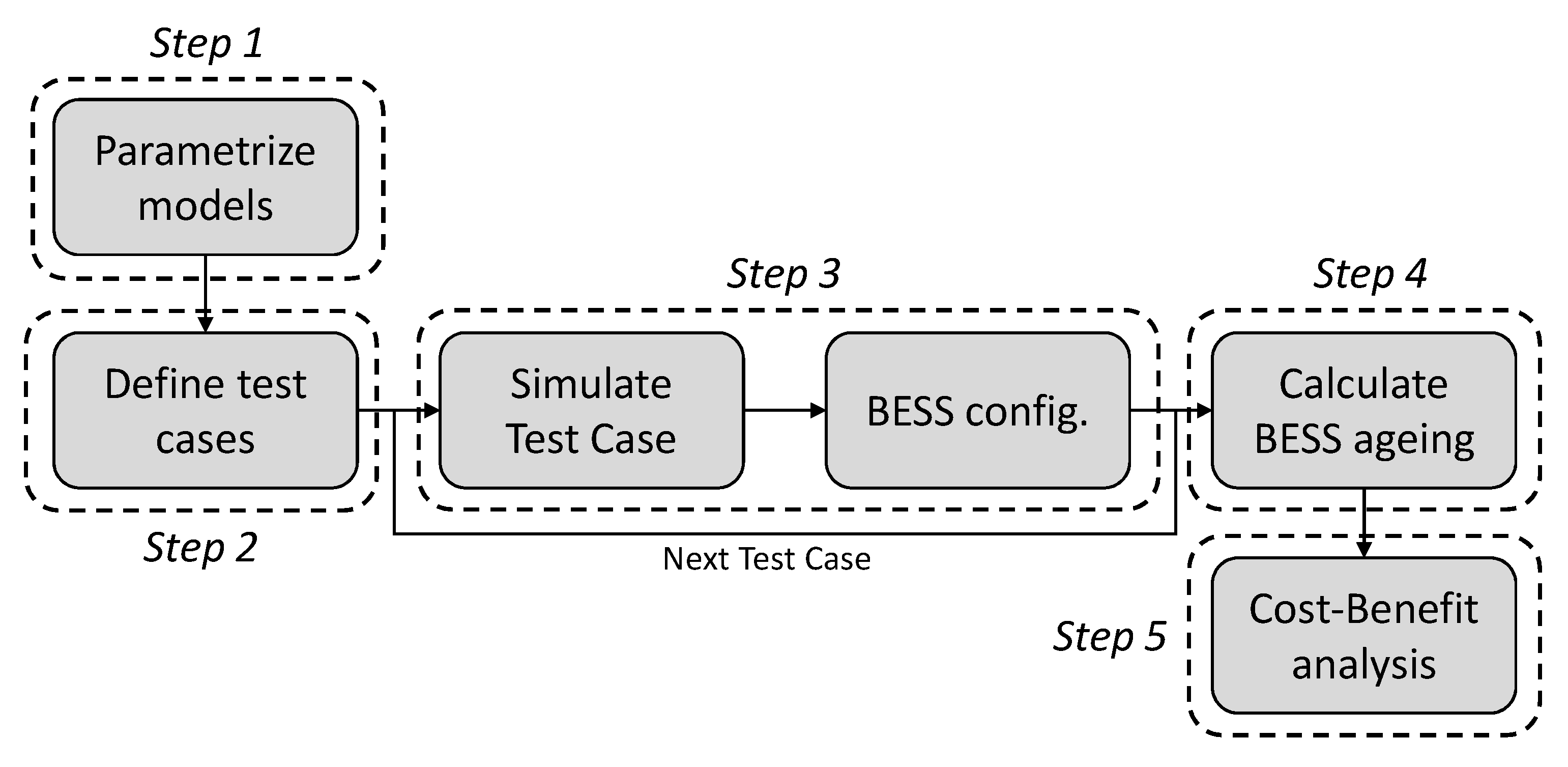
The methodology comprises a set of steps, as seen in the flow chart of
Figure 1.
Step 1: Models parameterizations. The different models, which are mathematical representations of physical systems or devices, account for variables (inputs and outputs) and parameters. In order to particularize the models (grid, BESS, and industrial consumption) to a specific system or device, those parameters must be adjusted to a fixed value.
Step 2: Define test cases. The variable that defines the test cases is the maximum fixed power that the grid can deliver (). Reducing this power limit implies adding a greater contribution from the BESS, which yields to the different scenarios, which consequently will result in different BESS configurations and different BESS ageing.
Step 3: Simulate test case, calculate BESS requirements, and BESS configuration. Once the scenarios have been defined, a simulation is performed for every value of . Each scenario implies different necessities from the BESS, regarding power and energy. This requirements give different BESS configurations, in terms of number of cells in series and in parallel. The charge/discharge profile for the BESS is also obtained from the simulation. If the energy available for charging is unable to match the amount of energy dispatched by a BESS in a specific scenario, that scenario will not be considered for the dimensioning process. As previously noted, this situation will force the BESS to, eventually, not being able to feed the load when the scenario repeats over time.
Step 4: Calculate BESS ageing. Once the minimum BESS configuration that satisfies the power and energy requirements is selected for each scenario, a BESS ageing analysis is performed, based on the BESS model and configuration, and on the charge/discharge profile for each specific scenario. As a result of this step, the number of days until the BESS loses a 20% of capacity retention is obtained.
Step 5: Cost–benefit analysis. Prices and fees for both a BESS (as a function of the kW and kWh of the system) and the fixed access power are needed for their incorporation into a cost function. BESS standard prices as well as Spanish fixed access rates are provided in
Section 4, with a case example. The cost can be computed yearly, taking into account the net present cost, and the capital recovery factor. The base scenario, i.e., when there is no BESS, is then compared to the rest of scenarios in terms of cost, and the final solution can be chosen.
3. Industrial Consumption, BESS, and Grid Modelling
The mathematical and simulation models used in
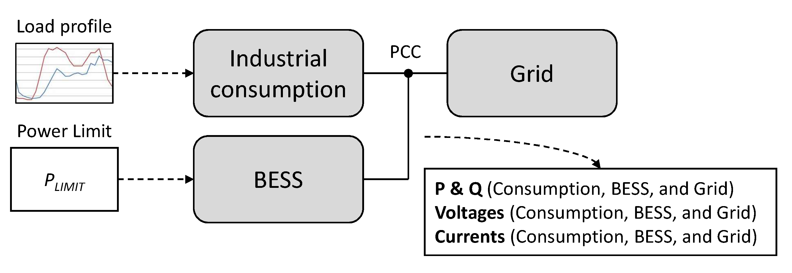
Section 4 for performing a case example of the aforementioned methodology are described in this section. Three main models are considered: an industrial consumption, a BESS, and a power grid. The BESS is connected to the same point as the industrial consumption, the point of common coupling (PCC), and both of them are connected to the grid, as it can be seen in the general model diagram in
Figure 2. The complete model outputs several electrical-variables time series (P, Q, V, and I) for the three main components. Additional electrical variables such as frequency or harmonic distortion are also evaluated and calculated by the model, but the authors decided not to output them since they are not relevant for the purpose of this paper.
The models are developed with MATLAB Simulink, under the Simscape Electrical environment. When developing simulation models, a higher complexity and completeness usually implies a higher accuracy [
17,
18]. However, complex models tend to require a substantial computational effort to run them, and a huge amount of information to parametrize them. Moreover, they are commonly valid only for a specific device, making them non-generalizable [
19,
20].
On the other hand, simplified models, usually composed by combination of resistors, inductors, and capacitors, are easily parametrized, they require low computational effort, and are valid for several devices with similar characteristics. Furthermore, even though they are not as accurate as complex models, they can mimic the behaviour of the device with sufficient precision, allowing for the extraction of general conclusions [
21,
22].
Hence, given the objective of this paper, the approach taken by the authors was to develop simplified models, that are generalizable and easily parametrized, which is sufficient for obtaining accurate general conclusions when dimensioning BESS.
3.1. Industrial Consumption Model
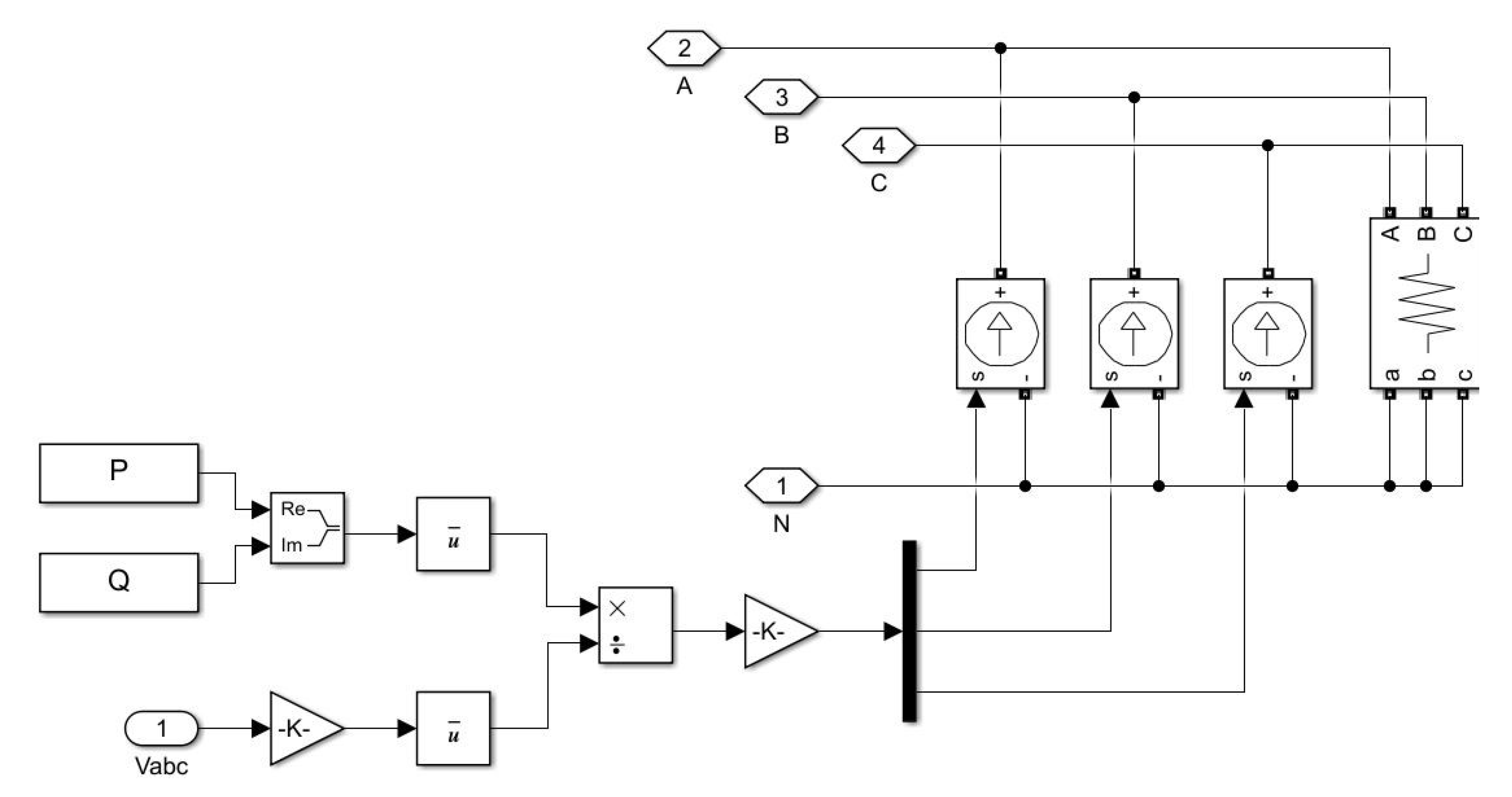
The industrial consumption is modelled as a PQ load, i.e., it consumes the desired active and reactive power independently of the voltage at the PCC. Hence, it needs to be modelled as a controlled current source, as depicted in
Figure 3. The inputs of the model, named as P and Q in
Figure 3, correspond to the 24-hour active and reactive power profile on a 1-second basis.
The Simulink diagram in
Figure 3 shows, from left to right, the inputs of the model P and Q together with the measured voltage (Vabc). From those inputs, the complex values of the phase currents are calculated, and then redirected to the corresponding current controlled source. A resistor with a very high value is also connected in parallel, which acts as a snubber. At last, the industrial consumption model is linked to the rest of the model via connectors A, B, C, and N.
3.2. BESS Model
The BESS model includes both a battery model and a power electronic converter model, the latter being necessary to manage the battery behaviour and to connect the battery to the AC grid.
3.2.1. Electronic Converter Model
For the purpose of this work, there is no need to model the power electronic converter in detail, since neither efficiency nor power converter ageing are incorporated into the economic evaluation of the methodology. Thus, an ideal voltage source converter (VSC) has been selected, with no conduction or switching losses and no power limitations, so the battery can dispatch as much power as required. As a result, the VSC is modelled as a controlled three-phase voltage source whose reference voltage is given by the converter control, which manages the power that flows in and out of the battery.
The control of a VSC can be modelled as explained in [
23], consisting of two levels: a high-level control and a low-level control. The high-level control is in charge of selecting, based on a specific strategy, the power dispatched or consumed by the battery. Several strategies have been proposed in the literature, from those based on rules [
24] to more complex strategies [
25,
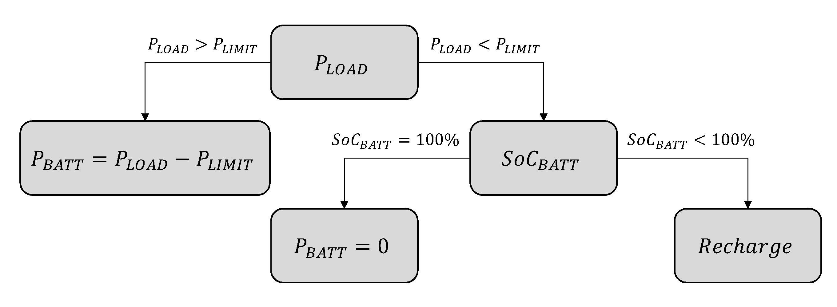
26]. For this paper, a simple strategy based on rules has been selected, which sets the reference power for the battery (
) based on the maximum power that the industrial consumption can absorb from the grid (
), the actual power that the industrial load is demanding (
), and the battery state of charge (
). The flow diagram for the high-level control is shown in
Figure 4.
The BESS recharge profile has been defined as the minimum current that allows the BESS to recharge the same amount of energy that it has provided to the load along the day. Moreover, reactive power reference for the battery has been set to zero, so no contribution is expected from it.
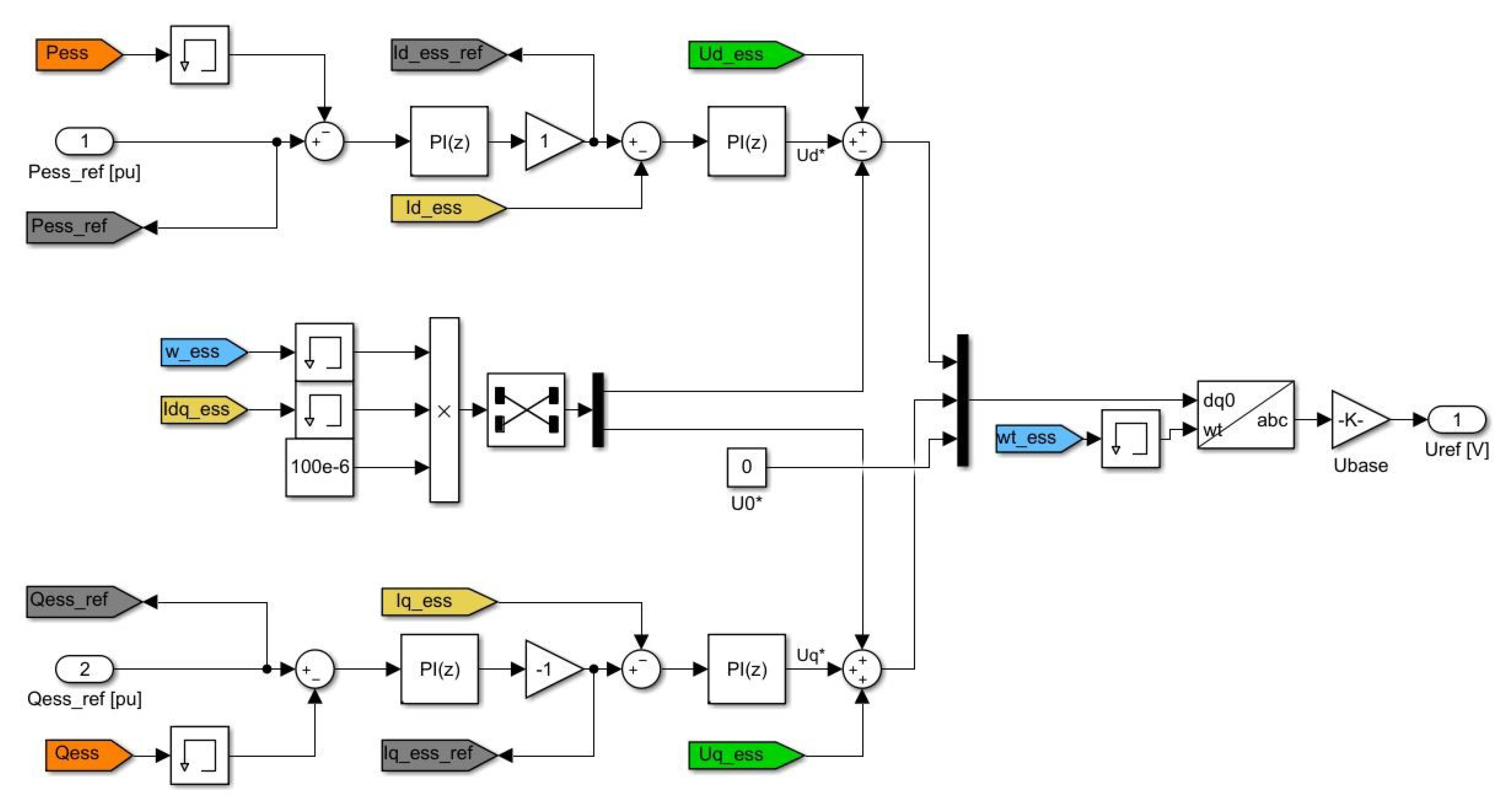
On the other hand, the low-level control is in charge of setting the voltage at the VSC terminals so that the power management commanded by the high-level control can be performed. The low-level control is a dq axis control, shown in
Figure 5, which has been developed building on [
27]. The control is duplicated for P and Q, with minor variations. Each branch accounts for an outer PI loop control, which sets the battery power equal to the reference power coming from the high-level control, outputting a reference current. Then, there is an inner PI loop control that adjusts the current flow through the VSC with the reference current, so a reference voltage is outputted. This voltage is finally regulated so that it corresponds to the VSC voltage at its terminals. In order to properly control the VSC, the inner control must be considerably faster than the outer control. Detailed explanation about the implemented dq axis control for a VSC can be found in [
23,
27].
3.2.2. Battery Model
The battery model controlled by the VSC is represented as an equivalent circuit model which, as mentioned above, sacrifices accuracy in favour of generality. Nevertheless, equivalent circuit models account for errors lower than 5% [
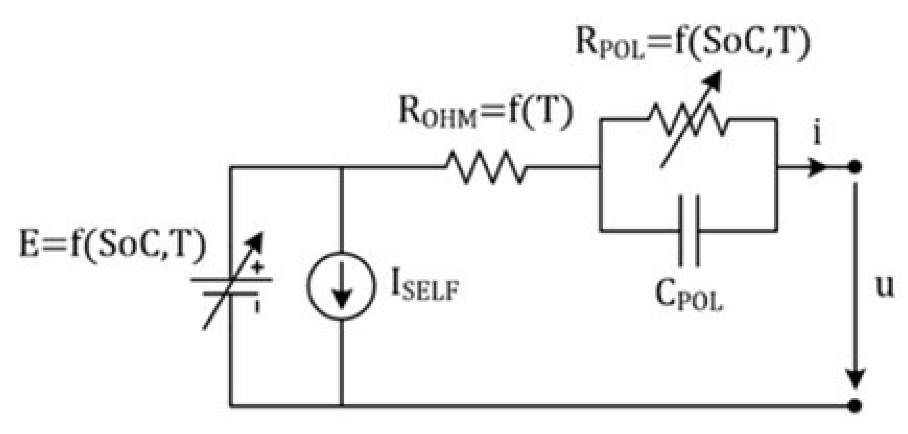
28], sufficient for obtaining general conclusions. The battery equivalent circuit is depicted in
Figure 6, where
u is the instantaneous battery voltage [V],
i is the battery current [A] (
i > 0 discharging;
i < 0 charging),
is the self-discharge current,
is the ohmic internal resistance [
],
is the polarization internal resistance [
], and
is the polarization capacitor [F].
The selected battery model has been developed and validated by the authors in [
18,
29]. The model comprises three parts: a voltage/runtime model, a thermal model, and an ageing model.
Battery Voltage/Runtime and Thermal Model
The lithium-ion battery model used in this paper is a modification of the MATLAB Simulink model in [
30]. The battery equivalent circuit is based on the Shepherd equation [
31], which was experimentally validated later in [
32]. The Shepherd model keeps the error between 1% and 5% and it can be parametrizable without testing the battery in the laboratory: it suffices with the manufacturer datasheet information. For the work developed in this paper, both voltage/runtime and thermal models have been parametrized via a least-square method. Data can be obtained from typical manufacturer’s curves: voltage-capacity curve as a function of different C rates (with constant temperature), and voltage-capacity curve at different temperatures (with constant C rate). The detailed parametrization process is described in [
33]. The voltage/runtime equations that govern the model, considering thermal dependencies, can be written as follows:
where
E is the open-circuit nonlinear voltage (V),
is the open-circuit constant voltage (V),
K is the polarization parameter (Ah
),
is the maximum capacity (Ah),
A is the exponential voltage constant (V),
B is the exponential capacity constant (Ah
),
T is the temperature (K),
is the parameter reference temperature (K), and
is the state of charge (%).
The thermal model comprises two different parts: a heat generation model and a heat evacuation model. The heat generation model can be expressed as follows [
34]:
where
H is the generated heat (W), and
the change of the equilibrium potential with temperature (V·K
).
The heat evacuation model occurs due to convection and radiation mechanisms, the latter being negligible [
35]. Assuming that the temperature in the battery is uniform (reasonable approximation according to [
36]), the following expression is obtained [
35]:
where
m is the mass of the battery (kg),
is the specific heat capacity (J·kg
K
),
h is the convective heat transfer coefficient (W·m
K
),
is the external surface area (m
), and
is the equivalent thermal resistance with the ambient (K·W
).
Hence, the temperature variation can be calculated as:
where
is the thermal time constant (s), and
s is the Laplace complex frequency parameter.
Battery Ageing Model
The ageing estimator implemented in the battery model comprises two parts: a cycling ageing model and a calendar ageing model. In order to parametrize both models, a least-square method has been applied, so the error between the model output and the real battery data is minimized. The data for parametrizing the models need to be obtained from experimental tests. The complete parametrization process is detailed in [
33]. A minimum set of 4 tests at different SoC and temperature are needed for the calendar ageing, and a minimum of 5 tests with different combinations of C rate, DoD and temperature are needed for the cycling model. Cycling ageing is related to the capacity fade when the battery is subject to charging and discharging cycles, i.e., when the current is flowing through the battery. It depends on several factors, among which
, temperature, and DoD are the most relevant [
37]. The cycling ageing model published in [
38] for lithium-ion batteries has been implemented:
where
is the cycling loss capacity (Ah),
the Ah that have flown through the battery (in or out), and
a,
b,
c,
d, and
e are constants depending on the battery chemistry.
On the other hand, calendar ageing is related to the capacity fade in the battery because of the time passed from the moment it was manufactured. It is dependent on the
of the battery, the temperature, and the time [
37]. The calendar ageing model published in [
39] has been implemented:
where
a,
b, and
c are constants that depend on the battery chemistry, and
z can take values between 0.5 and 1 and depends on the chemistry as well.
Apart from the ageing factors previously mentioned, additional ageing factors such as DoD or mean SoC along a cycle are indirectly considered by the model. The Ah dependency included in the cycling ageing is indirectly considering the DoD, since the higher the DoD the higher the Ah that flow through the battery. Moreover, the mean SoC along a cycle is considered in the calendar ageing equation, since the latter is constantly computing the battery SoC contribution.
3.3. Grid Model
The grid is modelled as an infinite power grid, so both the frequency and voltage at the PCC are kept constant. A Three-Phase Source model has been selected for this purpose, with a swing generator type, high short-circuit power, and low X/R ratio.
4. Case Example
In order to illustrate how the described methodology could be implemented, a case example is analysed. The models developed in
Section 3 are used for performing the simulations. The same structure of steps defined in
Section 2 is applied:
4.1. Step 1. Parametrize Models
At first, the simulations models need to be parametrized. For the grid model, the following parameters have been selected, so an almost infinite power grid is implemented (
Table 1).
The battery model can be parametrized following the methodology defined in [
29,
32,
33]. A commercial lithium polymer battery cell from Kokam, model SLPB100255255HR2, has been selected for this case study, which is a standard lithium-ion pouch cell [
40]. The experimental data for calculating the ageing model parameters have been obtained from [
40] and [
33], where the complete theoretical and experimental validation for the selected battery cell has been performed. The battery ageing model performs with an error below 5%, as detailed in [
33]. The selected battery cell main parameters are shown in
Table 2.
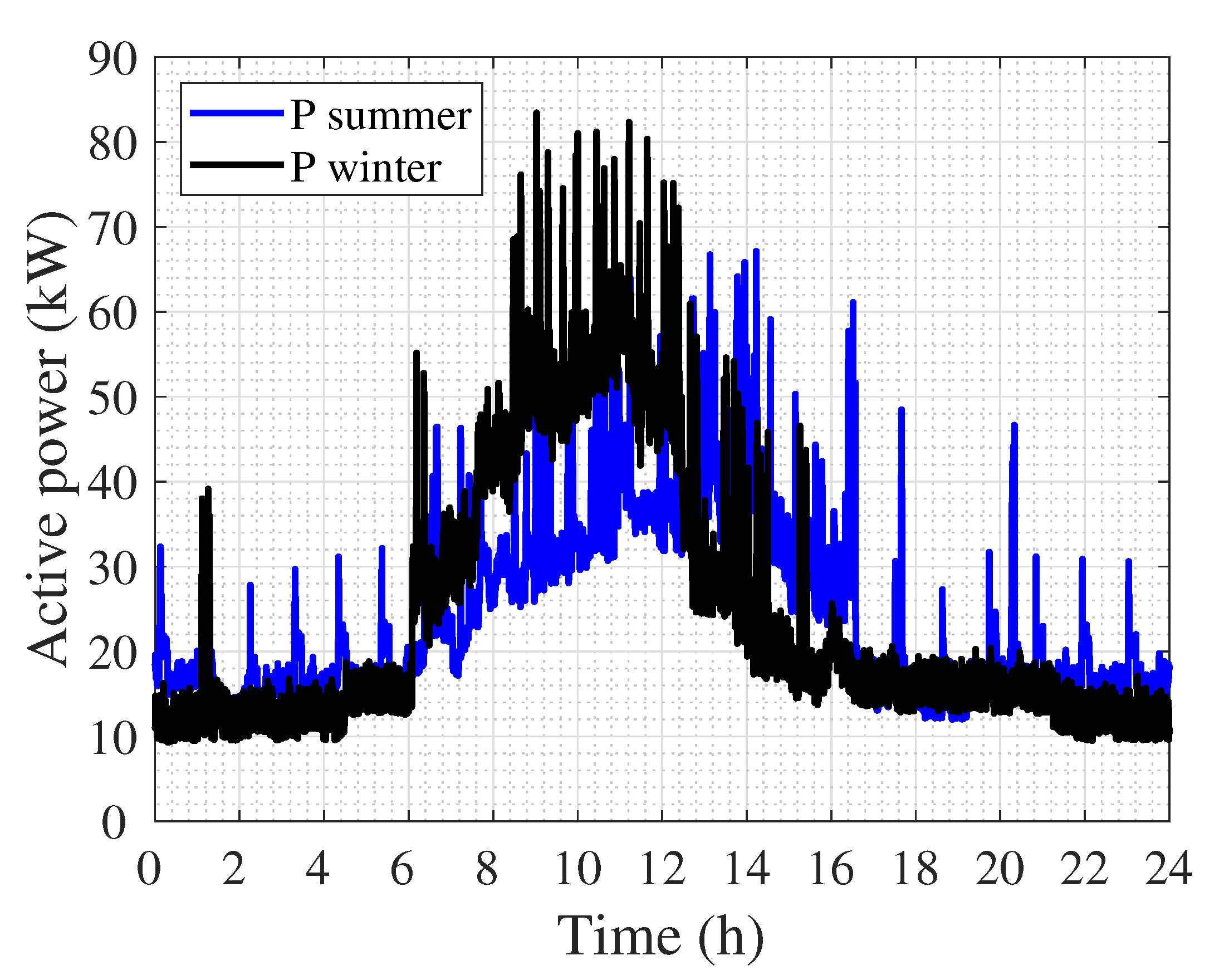
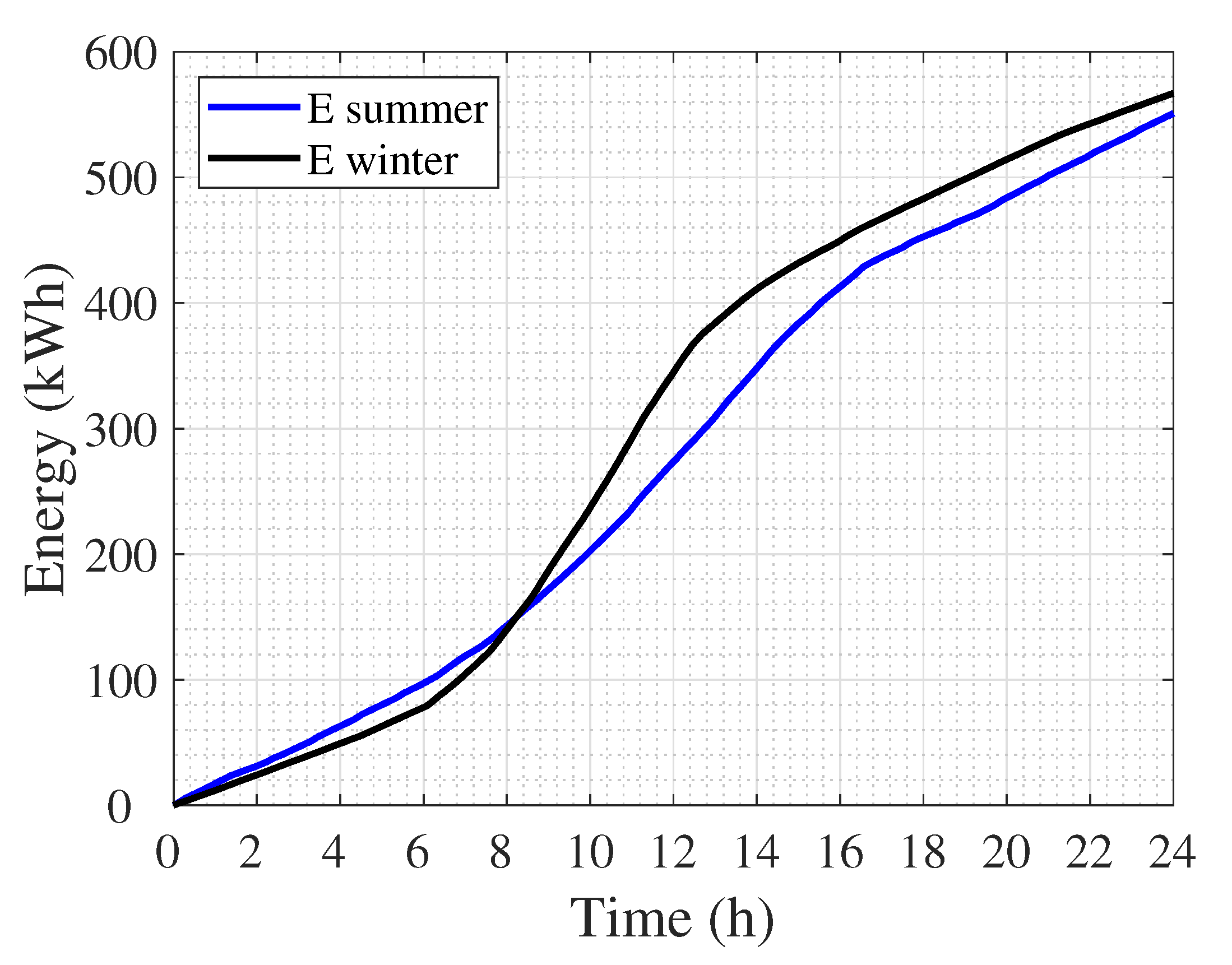
The load needs a power consumption profile as input. For this case example, two 24-h profile on a 1-second basis have been selected, corresponding to a typical day in summer and a typical day in winter in an industrial building. The selected building is the CEDEX facility in Madrid, located at Julián Camarillo 30, 28037 Madrid (Spain). For the analysis performed in this paper, the load corresponds to a three-phase load with no unbalance between phases, whose active power profiles are shown in
Figure 7 for both summer and winter. The cumulative energy consumed by the load for each typical day is also shown in
Figure 8.
4.2. Step 2. Define Test Cases
Test cases are defined by the BESS control parameter, which is the power limit that the load is allowed to consume from the grid (
). Hence, as
decreases, the battery will increase its contribution. Scenarios are divided between summer scenarios (S) and winter scenarios (W). SB and WB correspond to the base case scenario for each season, which is the current scenario at the real world facility, with a contracted power of 90 kW. Steps of 10 kW have been selected, so the different scenarios are defined in
Table 3.
4.3. Step 3. Simulate Scenarios and Obtain BESS Requirements and Configuration
As previously explained in
Section 2 and
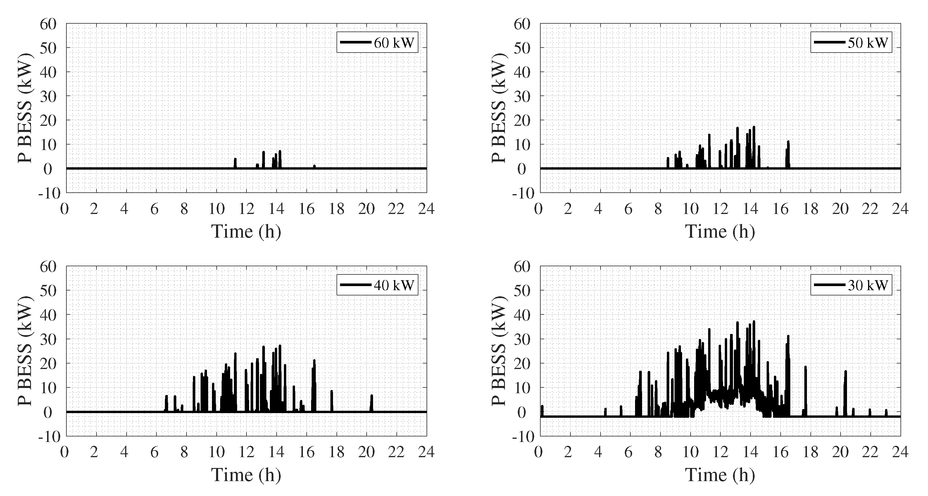
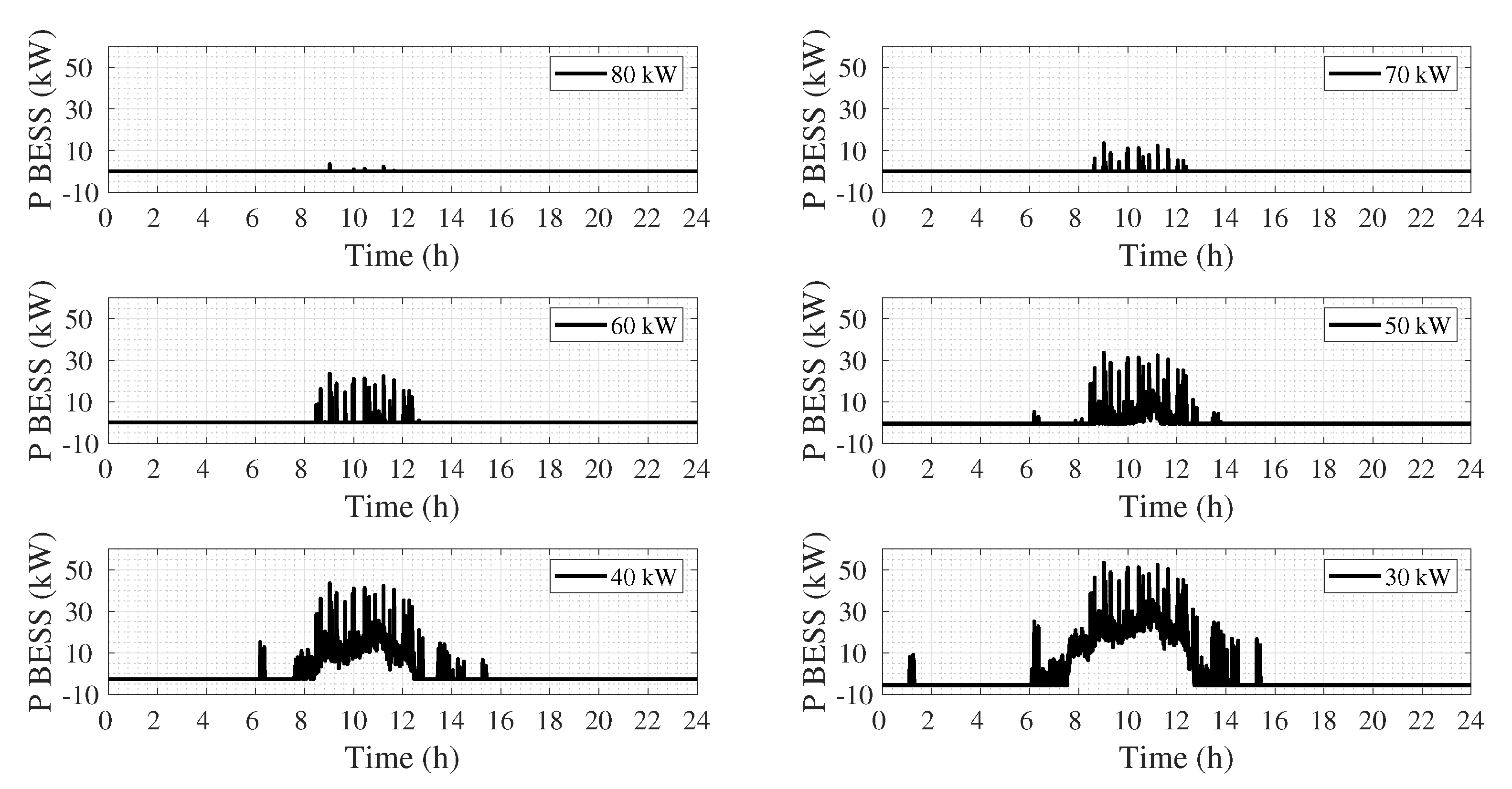
Section 3, BESSs that are not able to recharge as much energy as they have delivered along the day, are considered as not valid. Once the simulations are performed, BESS power profiles for the valid configurations are obtained. For the case example presented in this paper, valid BESS power profiles are shown in
Figure 9 and
Figure 10.
As expected, the lower the , the higher the contribution from the BESS. Since the BESS deals with high demand peaks, it follows a similar distribution as the top part of the industrial load profile for the corresponding scenario. Scenarios SB and WB, i.e., when the grid delivers as much power as demanded by the load, implies no contribution from the BESS.
For values below 30 kW, BESSs are not able to recharge the same amount of energy delivered during the high-demand period, both for summer and winter scenarios. It must be noticed that also affects the maximum power available for recharging, i.e., for a value of 20 kW, the maximum power available for recharging is 20 kW since that recharging power is coming from the grid, which is not sufficient for the case with values below 30 kW.
Based on the BESS power profiles, the power and energy requirements (
and
) for the valid scenarios are shown in
Table 4.
Once the requirements are calculated, the most suitable BESS configuration must be selected for each scenario (number of cells connected in series and in parallel). Commercial three-phase inverters for 400 V grids demand 48 V in the DC side. Hence, based on the standard cell parameters, the number of cells in series so the DC side voltage reaches 48 V equals:
The number of cells in parallel depends on the BESS energy requirements. Given that one branch of 13 cells accounts for:
The following table can be filled:
Table 4.
BESS requirements for the different scenarios.
Table 4.
BESS requirements for the different scenarios.
| Scenario | | | | Min. BESS Config. | |
|---|
| - | [kW] | [kW] | [kWh] | - | [kWh] |
|---|
| SB | 70 | - | - | - | |
| S6 | 60 | 7.13 | 0.015 | 13s1p | 2.64 |
| S5 | 50 | 17.13 | 0.12 | 13s1p | 2.64 |
| S4 | 40 | 27.13 | 2.07 | 13s1p | 2.64 |
| S3 | 30 | 37.13 | 34.79 | 13s14p | 36.96 |
| WB | 90 | - | - | - | |
| W8 | 80 | 3.45 | 0.01 | 13s1p | 2.64 |
| W7 | 70 | 13.45 | 0.05 | 13s1p | 2.64 |
| W6 | 60 | 23.45 | 0.43 | 13s1p | 2.64 |
| W5 | 50 | 33.45 | 11.51 | 13s5p | 13.2 |
| W4 | 40 | 43.45 | 49.78 | 13s19p | 50.16 |
| W3 | 30 | 53.45 | 101.14 | 13s39p | 102.96 |
Scenarios S6 to S4 and W8 to W6 can satisfy their energy requirements with just one BESS branch in parallel. It must be noticed that, given the BESS configuration and the power demand shown in
Table 4, the BESS in scenario S4 will be more demanded than in scenarios S5 and S6, and the BESS in scenario W6 will also be more demanded than scenarios W7 and W8, i.e., it will work with higher C rates.
4.4. Step 4. Calculate BESS Ageing
BESS ageing is closely related to its C rate and temperature (among other factors), as previously explained in
Section 3. The higher the C rate, the higher the temperature augmentation in the battery. Hence, the BESS configuration has a huge influence on the BESS ageing, since batteries with a higher number of cells in parallel work with lower C rates, i.e., with less stress. This implies that “bigger” BESSs may last longer than “smaller” BESSs, which may be beneficial from a cost–benefit point of view.
Four configurations have been tested for each BESS: the minimum number of cells so that the energy requirements are satisfied, and three more configurations increasing one extra branch each time, so that the C rate is decreased.
Commonly, a BESS is considered as aged when it loses 20% of its capacity retention.
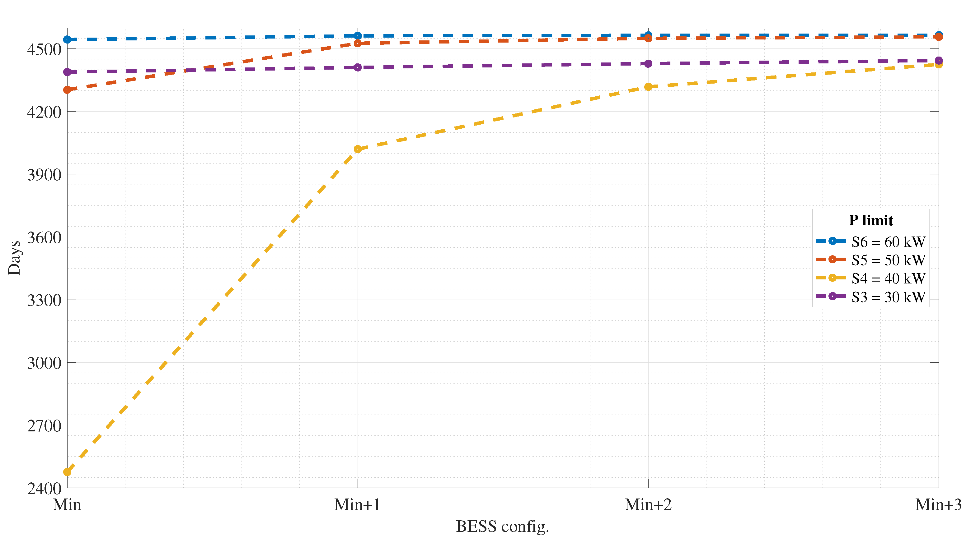
As seen in
Figure 11, Scenario S4 presents a very different behaviour from the minimum configuration to the minimum plus one. This happens because the C rate is diminished to a half when the branches in parallel are increased by one (from 1 to 2), which is a big difference according to the ageing model. A higher number of branches in parallel do not improve that much the behaviour, although the ageing is further reduced, as expected.
Scenario S3, which is the summer scenario with more energetic demand from the BESS, does not present a high ageing. This happens because the highest C rates are close to 1C, and there are few moments where those C rates are reached, even though the BESS is dispatching power during longer periods along a day. However, ageing for Scenario S3 is higher than Scenario S6, the BESS is working with a less intermittent profile, implying that temperature is higher during a cycle. Scenario S5 presents a higher ageing that Scenario S3 for the minimum BESS configuration, given that the C rate is higher (close to 3C), although it works for shorter times with that C rate. In any case, a low ageing is expected for every scenario except for Scenario S4.
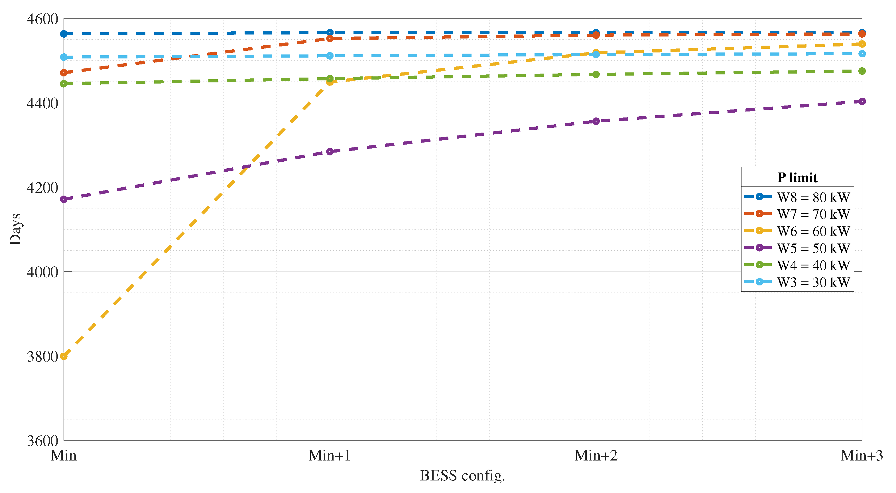
For winter scenarios, as seen in
Figure 12, Scenarios W8 and W7 present a low ageing due to the few periods of time under which the BESS is dispatching power, even though the C rate for W7 and the minimum BESS configuration reaches 5C. Besides, a low ageing is expected for Scenarios W3 and W4 which, being the most energetic form the point of view of the BESS, are hugely over-dimensioned in terms of power (very low C rates).
Scenario W6 presents a similar behaviour as S4, where increasing the number of branches in parallel from 1 to 2 prevents from an excessive ageing, which is produced as a consequence of working with C rates higher than 8C for a few moments along a day. Scenario W5 steadily improves its ageing as the branches in parallel increase, although it suffers from the highest ageing except for the minimum BESS configuration.
4.5. Step 5. Cost–Benefit Analysis
Once the BESS ageing for different configurations and scenarios has been calculated, a cost–benefit analysis must be performed, considering both the BESS cost and fixed term energy cost. Among the different reports found in the literature that analyse energy storage costs, the one published in [
41] has been selected as the most reliable study.
Moreover, electricity access fees for industrial consumption for the regulated market in Spain can be found in [
42]. The fixed term of the access fee considers three time periods of time-discrimination (P1, P2, and P3). For further information about the Spanish regulated market, and time discrimination periods, the authors recommend the work published in [
42].
The variable term of energy is kept constant for every scenario, i.e., the BESS is re-charged from the grid, and the BESS energy recharged form the grid plus the industrial load demand matches the total energy consumed by the industrial load in scenarios SB and WB, so the overall energy consumption remains constant. Hence, it is not included in the cost. Costs are summarized in
Table 5 [
42].
Considering this, the cost equation can be written as:
The contracted power () is considered constant for the three time-discrimination periods (as is requested to industrial consumption).
The yearly BESS project cost has been calculated based on [
43,
44,
45]. The annualized cost of the BESS project has been defined as:
where
is the annualized cost,
is the net present cost, and
is the capital recovery factor, which depends on the annual real discount rate (
i) and on the project lifetime (
).
is calculated as the present value of all the costs of installing and operating the battery over the project lifetime, minus the present value of all the revenues earned over the project lifetime.
Hence, the total yearly cost is calculated as follows: -4.6cm0cm
The constants for calculating the BESS project cost are listed in
Table 6 [
41,
43],
Table 6.
Summarized costs for the BESS project.
Table 6.
Summarized costs for the BESS project.
| Item | Value [Unit] |
|---|
| BESS cost (€/kW) | 1876 €/kW |
| BESS cost (€/kWh) | 469 €/kWh |
| 10 €/kW and year |
| i | 3.41% |
| 25 years |
where
is the operation and maintenance cost, and
is the number of years over which the cost is annualized. The total cost for each scenario is shown in
Table 7 and
Table 8, where:
As it can be seen in
Table 7 and
Table 8, results indicate that introducing a BESS into an industrial consumption for diminishing the fixed term of the electricity fee, can reduce the overall yearly cost. Moreover, this reduction can enhance an intelligent use of the energy in industrial buildings, as well as the improvement of the energy efficiency along the electric power grid, since consumption peaks are eliminated.
Table 7 and
Table 8 show that the minimum reduction in the fixed power limit is the best solution for this particular case example, both for summer and winter, from the point of view of the industrial consumer. Every configuration in scenario S6, and two of them in Scenario S5, reduce the yearly price of having a higher contracted power in summer. A similar behaviour is obtained in
Table 8 for Scenarios W8, W7 and W6. The rest of the scenarios do not improve the yearly cost for this case example, although some interesting conclusions can be drawn.
Scenario S4 shows that the minimum configuration might not be the optimal solution, since configuration 13s2p provides a higher cost reduction than the minimum BESS configuration. A higher number of branches in parallel allows for a reduced C-rate, DoD, and temperature in each scenario. Hence, the BESS lifespan is extended and a higher cost reduction is achieved. A similar result would be expected for Scenario W6, given the ageing behaviour shown in
Figure 12. However, in this case, the ageing is sufficiently low with the minimum BESS configuration, so the extra benefit of the further reduction in ageing does not improve that much the yearly cost.
Costs are not reduced in scenarios S4, S3, W5, W4, and W3 with respect to the base case scenario, since the BESS is dedicated not only to reducing the peak consumption, but to dealing with an important part of the load demand. This forces an over-dimensioning in the BESS’s number of cells in parallel (given that the number of cells in series is fixed), and indicates that those BESS configurations may not be the best option for feeding an industrial infrastructure by themselves since, even though technically viable, it is costly.
5. Conclusions
This paper presents a BESS dimensioning methodology for reducing the fixed term of the electricity access fee for industrial consumption, considering battery ageing and the cost of the BESS and electricity access fees. By connecting a BESS together with a consumption, the power demand peaks can be reduced, so there is no need for contracting a high fixed term power to cover the high demand peaks.
A five-step dimensioning methodology is described, finishing with a cost–benefit analysis to facilitate the final decision making. The methodology is easily implemented and can be adapted to different electricity market conditions, as well as particularized to different BESS or load conditions. The parameter that defines the different scenarios of the methodology is the power contracted from the grid, being the decision variable the combined cost of the BESS and the fixed electricity fee.
Results drawn from the two case examples show that implementing a small battery to limit the consumption peaks can lead to considerable cost reduction for the industrial consumer. In fact, the best techno-economical solution corresponds to a small BESS that limits the peak consumption. The low C rate, DoD, and steady temperature experienced by a BESS that only limits the top part of the peak consumption, guarantees a long lifespan that highly reduces the overall yearly costs. Given that BESS are over-dimensioned in energy in several scenarios (S6, S5, W8, W7, and W6), a higher contribution from the BESS could be imposed in order to reduce the fixed power contracted from the grid, achieving a higher peak reduction. However, this leads to an increased ageing (higher C rate, DoD, and temperature profile) that has an impact on the techno-economical decision, turning those solutions into non-optimum.
Apart from the previous conclusion, depending on the case example and scenario under study, it could be beneficial from the economical point of view to increase the size of the BESS with more cells in parallel. This situation occurs when the BESS energy is suited to the BESS energy requirements (scenario S4). This forces the BESS to work with a high DoD and high C rates, deriving in a premature ageing. Thus, increasing the BESS size will allow it to work under less stress, extending the time needed to a BESS replacement and reducing the overall yearly costs.
One important conclusion drawn form the case examples results is that the optimum BESS is over-dimensioned in both power and energy. This may indicate that other energy storage technologies different than Li-ion batteries could be more beneficial from the techno-economic point of view. Supercapacitors, which can last millions of cycles until they need a replacement, or flow batteries, which can dissociate energy and power, may be suitable for their inclusion in a further study. In addition, if the industrial consumption is facing a scenario with low consumption peaks, the optimum solution could be discarding the usage of an energy storage system at all. As previously stated, the presence of high consumption peaks is the reason that justifies the inclusion of a BESS together with the industrial consumption.
Consequently, the proposed methodology is of potential interest for industrial consumers, since the cost-benefit analysis may reduce the yearly cost of their infrastructure, and also for TSOs and DSOs, since the peak reduction improves the efficiency of the transmission and distribution of the energy along the electric power grid. Moreover, BESS manufacturers could also find benefits in this methodology for the development of specific products related to this industrial demand peak and fixed term fee reduction.
Suggested future works include the parametrizations of the grid with frequency and voltage variations, so that further analysis considering BESS contributions to the grid in terms of frequency and voltage regulation can be performed. Moreover, time discrimination pricing can be added to electricity energy prices, so that the BESS can recharge during low price periods, providing an even higher reduction than the one shown in this work. At last, a techno-economic evaluation considering other energy storage technologies such as supercapacitors or flow batteries may result in interesting conclusions.


 ,
, 


