Modulation Linearization Technique for FM/CW SAR Image Processing Using Range Migration

Featured Application

The technique described herein is a method for linearizing the frequency modulation error of a Frequency-Modulated/Continuous Wave (FMCW) radar as part of range migration processing when forming SAR images that results in no additional computation cost.

Abstract

Linear FMCW radar suffers from impairments in range and range rate if there are errors in the modulation rate or phase discontinuities. Often, this is a result of a nonlinearity of the voltage-controlled oscillator that is in the source of the transmit and receive local oscillator. The nonlinearity can be corrected at the source by using a nonlinear control voltage or by processing the received beat frequency. Any signal processing using the later method leads to computation time and energy costs, which can be considerable in some applications. When the range migration algorithm using the Stolt Transform is used for Synthetic Aperture Radar (SAR) image processing, the autofocus linearization technique described here costs nothing in additional hardware or computation time.

1. Introduction

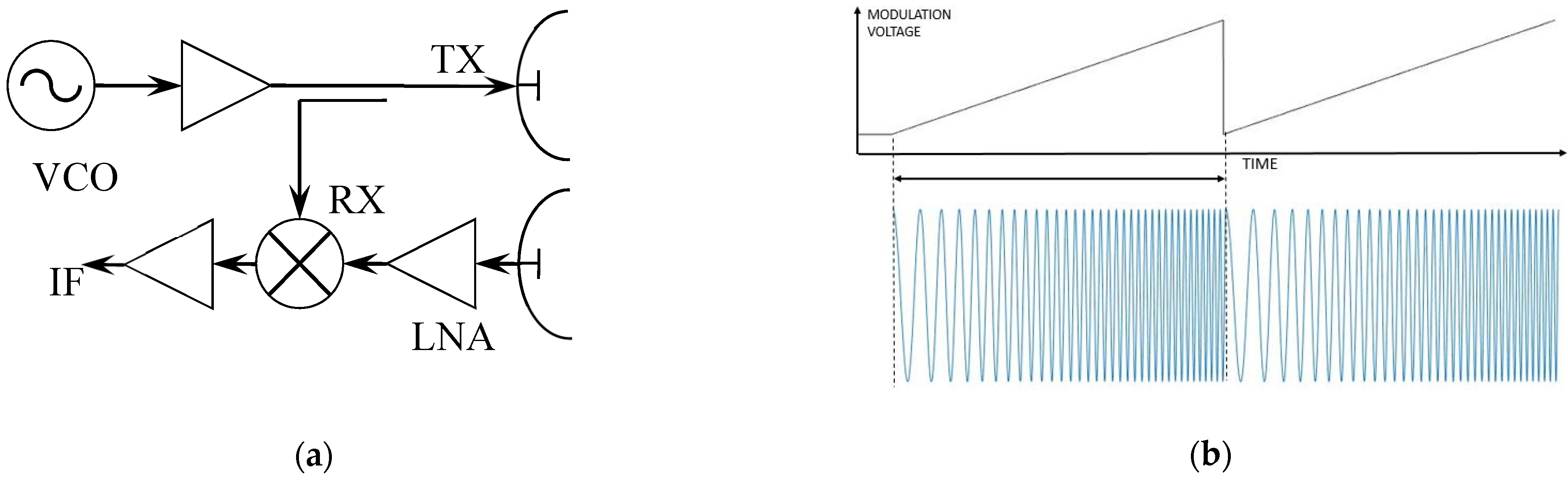
Much has been written about FMCW radar, especially using linear modulation [1,2,3,4]. These can be seen in block diagram Figure 1a, and in Figure 1b, which shows an example waveform where the desired modulation is a linear ramp from 400 MHz to 800 MHz

The transmitted frequency during a single linear sweep is

$${\omega }_t\left(t\right)=\frac{d}{dt}{\theta }_t\left(t\right)=2\pi m_{o}t+{\omega }_o$$

(1)

where

$${\theta }_t\left(t\right)=\pi m_o{t}^2+{\omega }_{o}t+\phi$$

is the instantaneous transmit phase, m_o is the modulation slope in Hz/s, t is time, ω_o is the frequency offset at the beginning of the ramp in rad/s, and φ is a constant phase angle in radians.

The phase of the received signal from a single point scatterer at a delay θr, is

$${\theta }_t\left(t\right)=\pi m_o{(t+\tau )}^2+{\omega }_o(t+\tau )+\phi$$

(2)

where θr(t) is the transmit or receive phase as a function of time, and τ is the round-trip time delay for a single point target. The received signal is a time delayed version of the transmit signal due to a radar scattering object. The transmit and receive signals are mixed and the baseband difference signal is kept for further processing.

$${\theta }_{\delta }\left(t\right)={\theta }_r\left(t\right)-{\theta }_t\left(t\right)=\left(\pi m_o{\tau }^2+{\omega }_o\tau \right)+2\pi m_{o}t\tau +{\omega }_o\pi$$

(3)

The discrete phase as sampled as In phase and Quadrature phase baseband signals can be expressed as

$${\theta }_{\delta }\left(n\right)=2\pi m_{o}nT\tau +{\omega }_o\left(\pi m_o{\tau }^2+{\omega }_o\tau \right)+\pi$$

(4)

where T is the sample period and n is the sample number. The frequency of the baseband signal is

$${\omega }_{\delta }=\frac{d}{dt}{\theta }_{\delta }\left(t\right)=2\pi m_o\tau$$

(5)

which would show up as a peak after taking the Fourier Transform of the sampled data.

It is also known that nonlinearity in the modulation, i.e., replacing m_o with m(t), results in a baseband frequency that is not constant over the modulation ramp. This is a common problem in FMCW radar where the signal source is a voltage-controlled oscillator (VCO), and does not have a linear voltage to frequency characteristic. If left uncorrected, defocusing in Synthetic Aperture Radar (SAR) images becomes worse, especially at large squint angles and wide bandwidths.

Solutions have been proposed and proven to compensate or correct for nonlinearities. These solutions require additional hardware such as a delay line [5,6], a Phase-Locked Loop [7,8,9], or Surface Acoustic Wave filter reference path delay [10,11]. Some methods require additional digital signal processing of the Intermediate Frequency (IF) [12,13,14]. The method described here utilizes phase resampling and integrates this with the Stolt interpolation in the Range Migration Algorithm.

2. Linearization Method

2.1. Linearization Using Resampling

Some promising solutions to correct single pulse data are time resampling [15,16] and phase resampling [17]. In terms of discrete samples, the phase of the baseband signal is given by Equation (4) above. If there were no modulation error, the change in the baseband phase would be only due to round-trip delay of a single point-target and the modulation slope

$$\Delta \theta =2\pi m_{o}T\tau$$

(6)

When there is modulation error, phase differs from sample-to-sample. The nth sample is given by:

$$\Delta \theta +{\phi }_n=2\pi (m_o+{ϵ}_n)T\tau$$

(7)

where ${ϵ}_n$ is the error in modulation slope at the time of the nth sample and φ_n is the phase error at the nth sample. The error term is

$${\phi }_n=2\pi \left({ϵ}_{n}T\right)\tau$$

(8)

which reduces to one error vector, (ε_nT), that can be expressed as a modulation error or a sample time error.

Time resampling, by interpolation, of each range profile effectively compensates for the phase error for at the cost of computation time [15,16]. Time resampling ratio can be fixed or optimized using phase error and the largest range of interest [17] by the least squares fit at calibration time.

Autofocus method as described by Middleton et al. [18] is accomplished by a measurement of a calibration target at a known range. The baseband signal should be a sinusoid, and the phase error is extracted. Note that the phase error is a function of time delay. Objects will be more out of focus the farther they are from the calibration range. Scatterers at different ranges would need a scaled version of this phase correction. A different matched filter can be applied to each range bin, but is not effective for practical scenes that include clutter and multiple objects.

2.2. Range Migration Algorithm in SAR Imagery

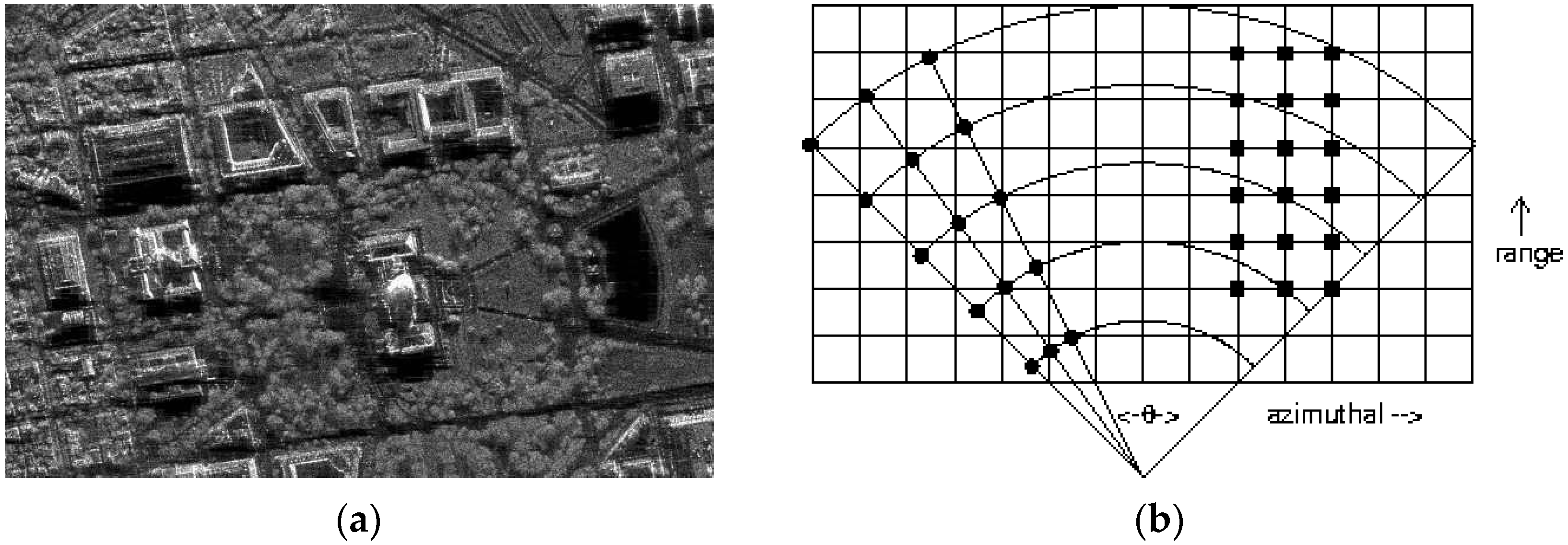
The Range Migration Algorithm (RMA) here has been previously described [19,20]. Consider an ideal SAR image and geometry in Figure 2 with the following properties: (1) the aperture is a straight line; (2) radar data are sampled at uniform intervals; (3) the image scene is broadside and centered on the aperture; (4) the radar antenna illumination is a constant amplitude plane wave.

At the beginning of RMA processing, the collected SAR signal history is range compressed, match filtered, and compensated for range skew if the data are from a pulse radar. This is not necessary for FMCW radar data. Then, range curvature is removed for scatterers at the center of the scene. This range curvature is recognized in the range profile as an arc with a quadratic phase characteristic.

The RMA operates on the two-dimensional complex phase space S(k_x,k_r) where k_r is the range phase space and k_x is the along-track phase space, if range compressed pulse data would require transformation to the phase domain by a Fourier Transform (FT) on the pulse-by-pulse data. The sampled data of an FMCW radar are already in terms of sampled phase, k_r, but should be windowed for a suitable method such as a Hamming window. If these data represent real only phase history, it is necessary to transform this into complex data by techniques such as a Hilbert transform or by an Inverse Fourier Transform (IFT) on the one-sided result of a Fourier Transform (FT). Finally, a one-dimensional FT taken in cross-range will yield the k_x along-track phase space.

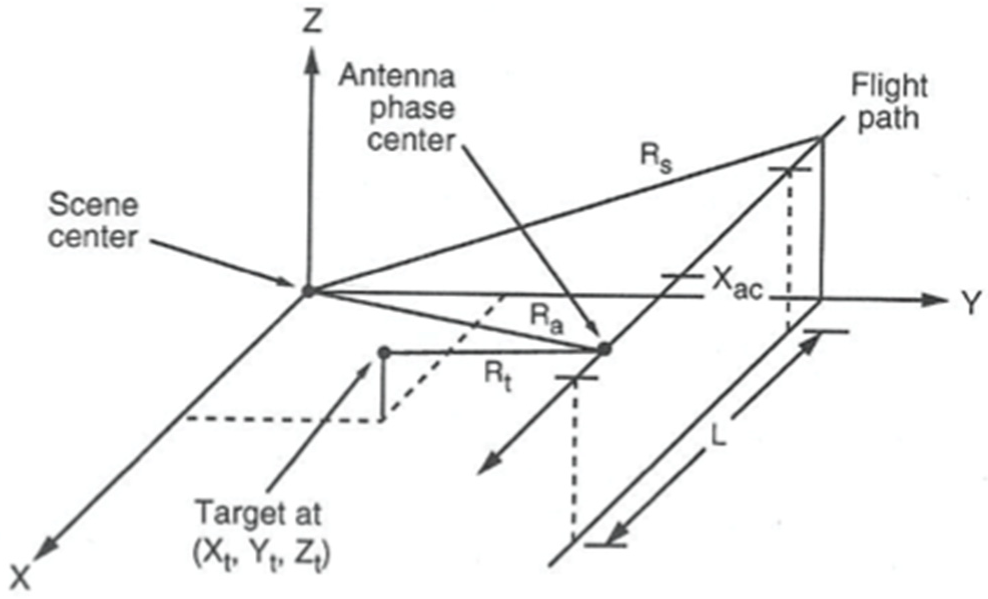
The second step is the application of a two-dimensional matched filter. This operation corrects for range curvature of all scatterers at the same range as the scene center. The phase of this two-dimensional matched filter is given by:

$${\mathsf{\Phi }}_{mf}\left(k_r,k_x\right)=-R_s{k}_r+R_s\sqrt{k_r^2-k_x^2}$$

(9)

where R_s is the slant-range to the center of the scene as shown in Figure 3 above. For scatterers at slant-ranges other than Rs, some curvature will remain.

For an ideal linear FM/CW radar, a point scatterer on the center line of the scene at R_s is a sinusoid in the k_r coordinate at every point along track corrodent k_x in the (k_x,k_r) domain. However, point scatterers at other ranges would have some residual curvature, i.e., the sinusoid stretches (in cases where the target slant-range is less than R_s), or compresses (if the slant-range is greater that R_s) as the user traverses in the k_x direction. On top of this curvature is the phase-error caused by a nonlinear VCO in the FMCW radar considered here.

The Stoltz transformation corrects this their residual curvature described above [21,22]. This transform is a convenient mechanism to also correct for phase-error. The Stoltz transform is a one dimensional mapping of (k_x,k_r) domain space into (k_x,k_γ) space by

$$k_{\gamma }=\sqrt{k_r^2-k_x^2}$$

(10)

This is implemented by interpolation, so the result is uniformly spaced samples k_r remain uniformly spaced in k_γ. If not, the resultant pixel size would vary in range across the image.

The final step in Range Migration Algorithm (RMA) is a two-dimensional Fourier transform that result in an image in range and cross-range. This would result in a well-focused image for an ideal radar.

2.3. Linearization in RMA SAR Processing

In practice, the phase error in Equation (8) above, as determined by a calibration target, only applies to scatterers in a Synthetic Aperture Radar (SAR) scene at the same slant range. The RMA process offers an opportunity to correct for the range-dependent phase error: in calculation and application of the matched filer Equation (9) or in the Stolt transform and subsequent interpolation of k_γ. By realizing that k_r is:

$$k_{\gamma }=\sqrt{k_r^2-k_x^2}-k_e$$

(11)

where k_e is the phase correction factor measured with a calibration target in Equation (8) and equal to

$$k_e=\frac{2 \left(\Delta r\right) }{R_c}{\phi }_n$$

(12)

The interpolation operation expressed by Equation (10) must be performed in the RMA image formation process, the addition of the phase correction term Equation (12) results in little to no cost in computation time or memory.

The calibration target at a distance R_c from the radar and Δr is the range resolution. The term k_e can be interpreted as the incremental phase error imposed by each range cell in turn and correcting for the roundtrip propagation. Keep in mind that the terms k_γ, k_x, and k_e are 1 by N arrays, where N is the number of data samples for each ramp (i.e., fast time).

3. Experimental Results

This technique was applied to 2.4 GHz FWCW SAR data taken with a low-cost radar and platform constructed by the authors in the same way as the previously published coffee-can radar [23]. The radar Voltage Controlled Oscillator (VCO) was purposefully driven over a bandwidth of 1.1 GHz, well outside its linear region. The radar was mounted on a cart and pushed along a straight line at a constant speed. Data were collected by a laptop and saved as a wave file.

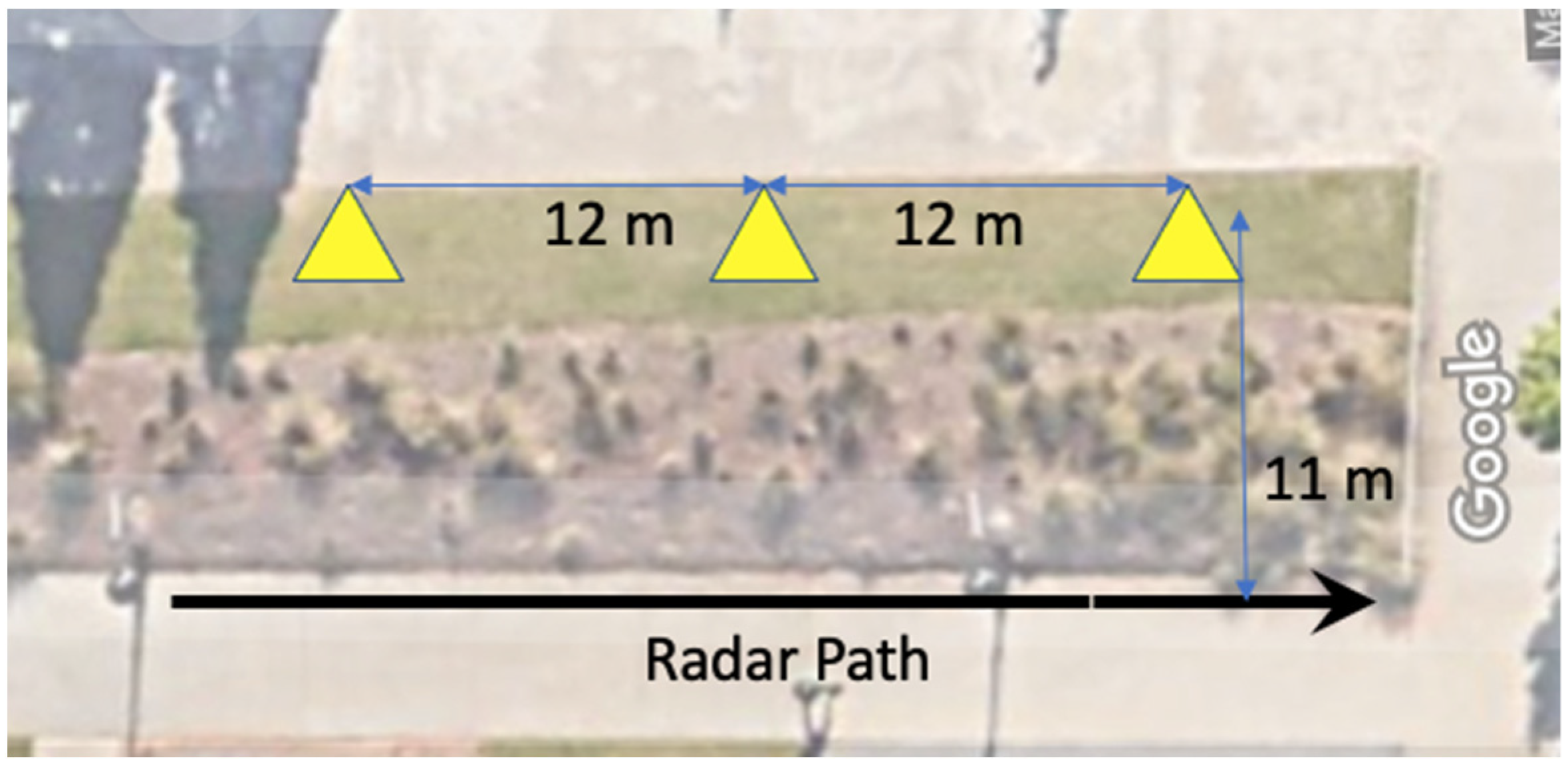
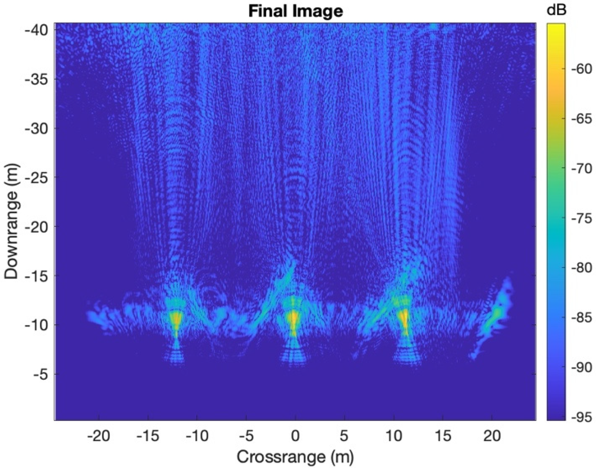
In the first experiment presented here, three corner reflectors were placed approximately 12 m apart, 5.5 m from the broadside track of the radar, as shown in Figure 4. SAR images were formed by taking the sampled data of one pass along a 50-m-long track marked ‘Radar Path’ in Figure 4. Data were stored and post-processed to form the SAR images shown here.

The sampled ‘IF’ voltage from one modulation ramp every 3.5 cm along the synthetic aperture was windowed with a Hanning window. Next a cross track Fast Fourier Transform (FFT) was calculated that resulted in the S(k_x,k_r) space. The RMA algorithm was used on that data without attempting to correct for modulation error. Figure 5 below shows the resultant image. The three corner reflectors stand out as the three bright returns but show considerable broadening in range due to the nonlinearity of the modulation.

To use the technique described here, using Equation (11) in the RMA, the phase error k_e can be found by autofocusing on one of the corner reflectors in the image by the same technique as described by phase resampling [21].

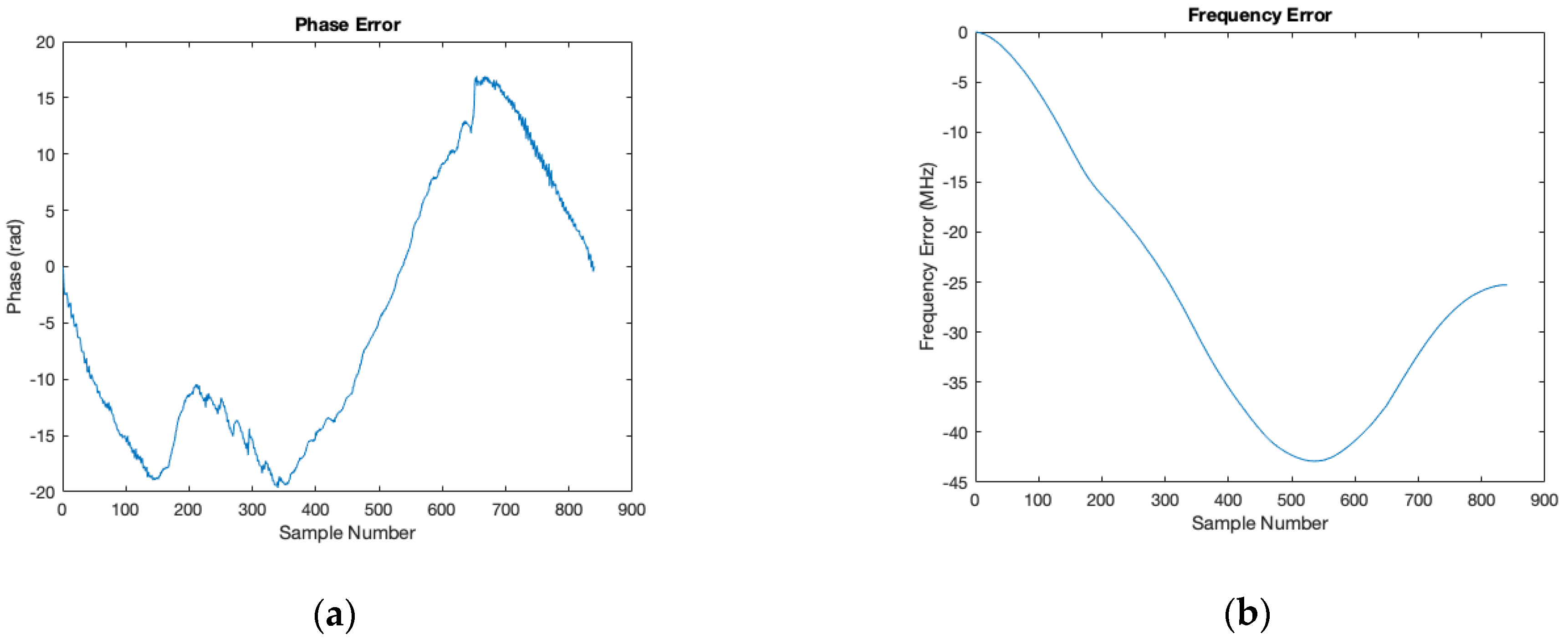
The corner reflector labeled as number 1 in Figure 4 was used as the calibration target to find the frequency and phase error shown in Figure 6. This phase error φ_n is used in Equation (12) to find k_e. This was then used as Equation (11) was substituted for Equation (10) in the Range Migration algorithm and Stolt Transform.

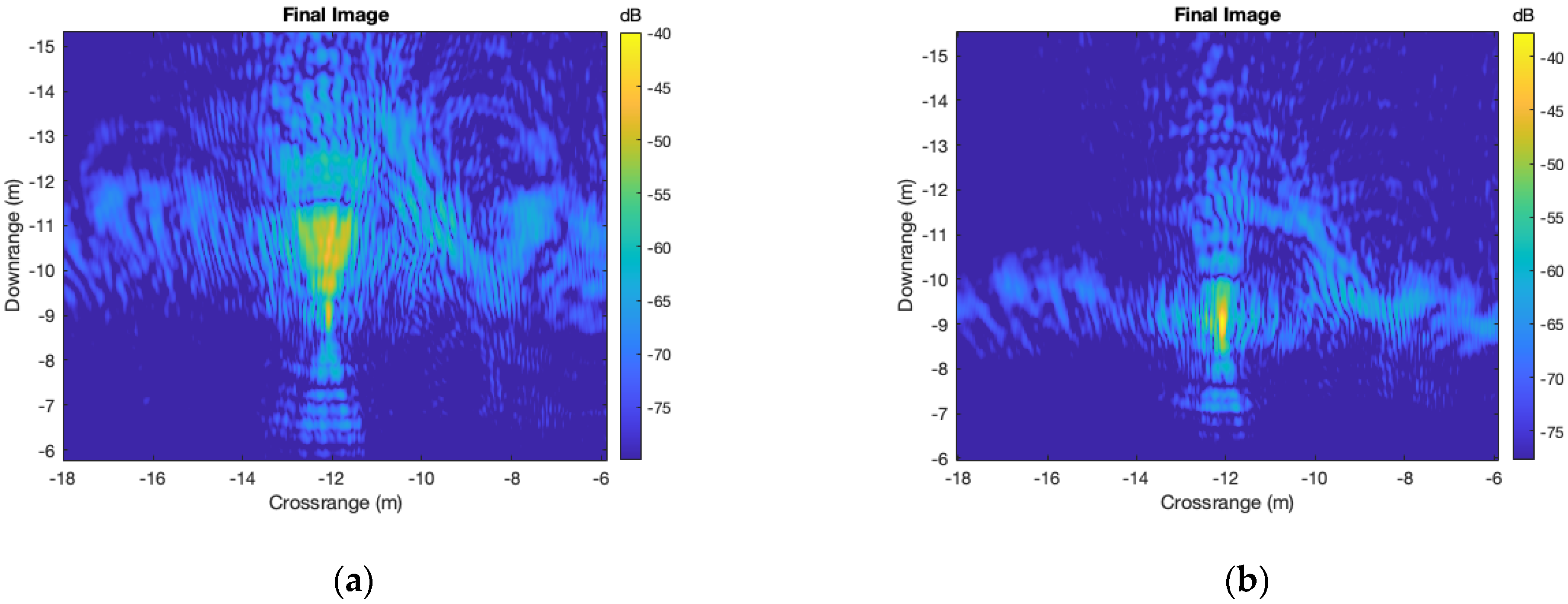
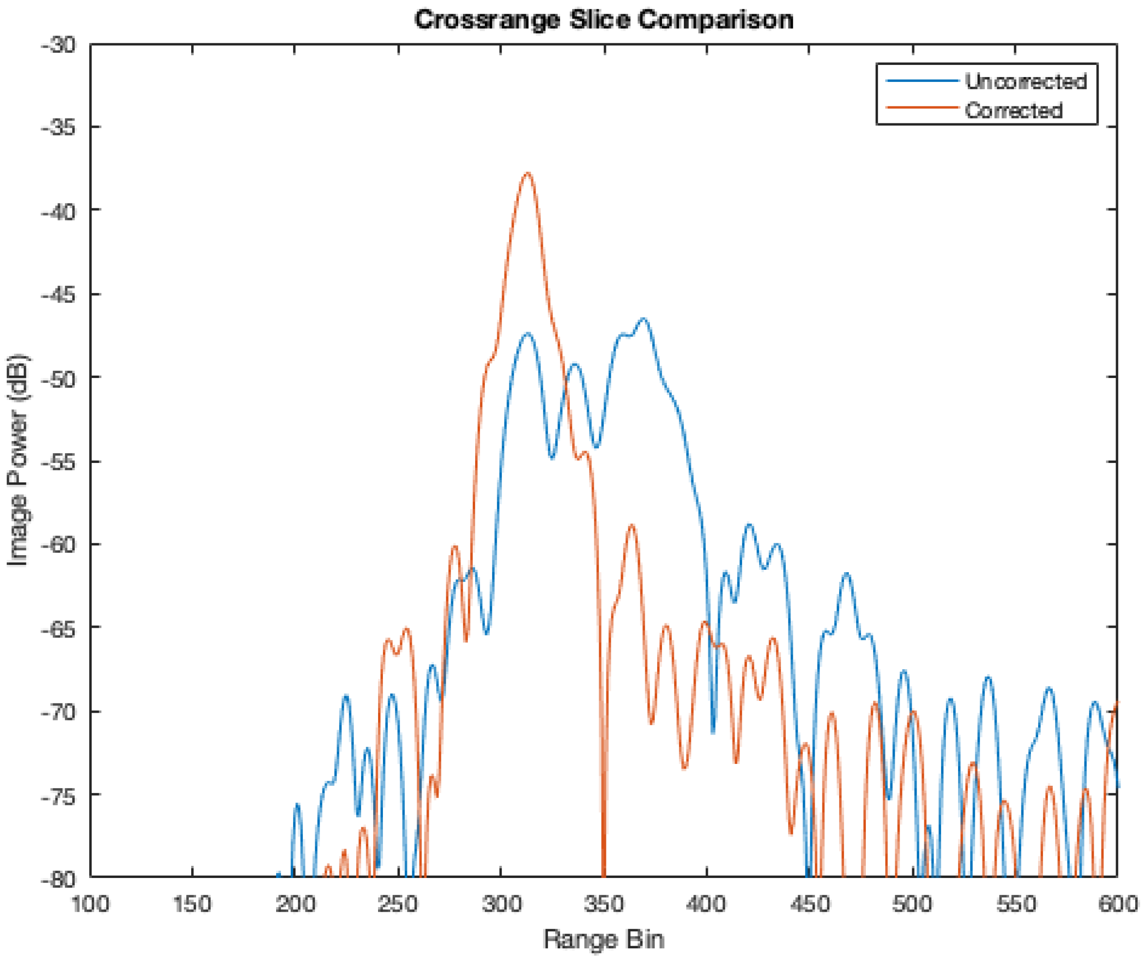
Figure 7a below shows a close up of the calibration reflector before error correction and Figure 7b shows two SAR images of one corner reflector before and after phase error correction using the technique described here. Figure 5 shows the image power of a range slice through the center of the peak.

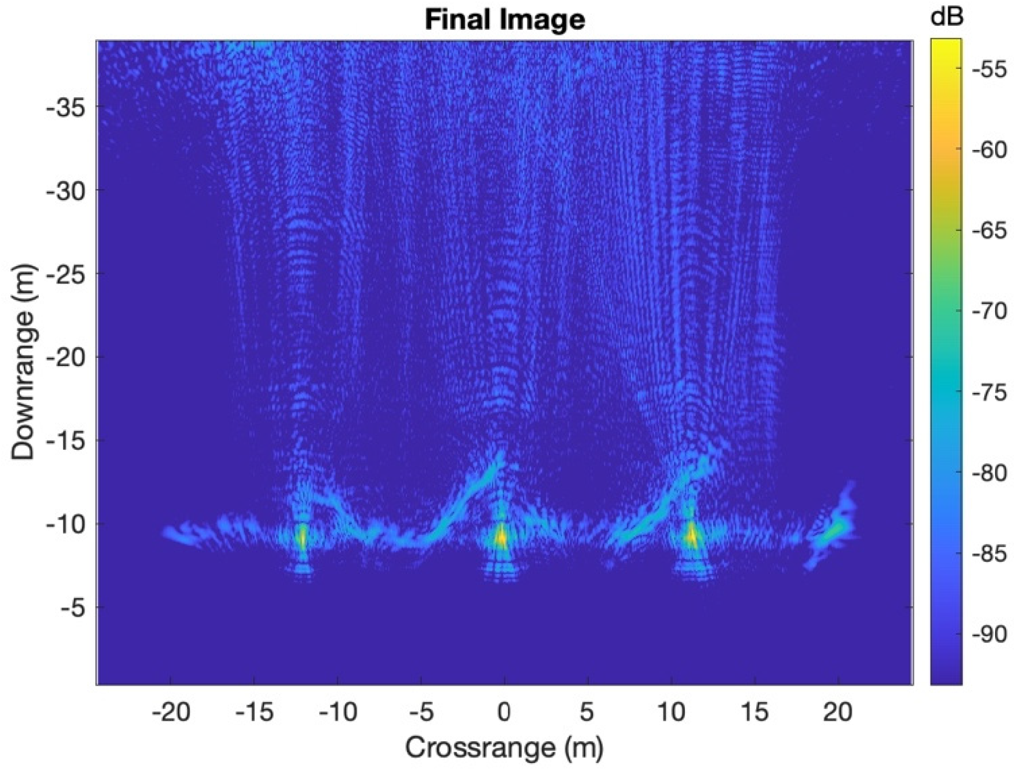
Figure 8 below shows the range profiles as a slice of the images through the peak at approximately 12 m from the center of the image. The uncorrected range profile is wide and contains multiple sidelobes. After the correction, the theoretical range resolution is achieved. Figure 9 shows the whole corrected image of all three corner reflectors showing that all have benefited from phase correction.

4. Conclusions

FMCW radars often suffer from nonlinear frequency modulation, which reduces the range resolution and image quality when used in a synthetic aperture radar. Previously reported methods of linearizing the modulation for SAR applications resulted in: (1) additional hardware; (2) an increase in the computational load; and (3) are only effective over a limited range extent.

The technique presented here results in little to no computational cost when the Range Migration Algorithm is used because the correction is a simple sum before the interpolation process needed by the Stolt transform. Once found, the phase correction applies to the full range extent that is expected from the Stolt transform. Given the fact that the phase error is found from experimental data using a calibration target, the anytime the modulation characteristics of the VCO, such as temperature or power supply voltage, the calibration will no longer be valid. The extent of the degradation will depend on the VCO’s response to these changes and the severity of the modulation error.

References

- Stove, G. Linear FMCW radar techniques. IEE Proceed. F 1992, 139, 342–350. [Google Scholar] [CrossRef]
- Piper, S.O. Homodyne FMCW Radar Range Resolution Effects with Sinusoidal Nonlinearities in the Frequency Sweep. In Proceedings of the 1995 IEEE International Radar Conference, Alexandria, VA, USA, 8–11 May 1995; pp. 563–567. [Google Scholar]
- Chen, W.; Xu, S.; Wang, D.; Liu, F. Range Performance Analysis in Linear FMCW Radar. In Proceedings of the 2nd International Conference on Microwave and Millimeter Wave Technology Proceedings, Chengdu, China, 14–16 September 2000; pp. 654–657. [Google Scholar]
- Brennan, P.V.; Huang, Y.; Ash, M.; Chetty, K. Determination of Sweep Linearity Requirements in FMCW Radar Systems Based on Simple Voltage-Controlled Oscillator Sources. IEEE Trans. Aerosp. Electr. Syst. 2011, 47, 1594–1603. [Google Scholar] [CrossRef]
- Fuchs, J.; Ward, K.D.; Tulin, M.P.; York, R.A. Simple techniques to correct for VCO nonlinearities in short range FMCW radars. In Proceedings of the 1996 IEEE MTT-S International Microwave Symposium Digest, San Franscisco, CA, USA, 17–21 June 1996; Volume 2, pp. 1175–1178. [Google Scholar] [CrossRef]
- Kang, B.K.; Kwon, H.J.; Mheen, B.K.; Yoo, H.J.; Kim, Y.H. Nonlinearity compensation circuit for voltage-controlled oscillator operating in linear frequency sweep mode. IEEE Microw. Guided Wave Lett. 2000, 10, 537–539. [Google Scholar] [CrossRef]
- Pichler, M.; Stelzer, A.; Gulden, P.; Seisenberger, C.; Vossiek, M. Phase-Error Measurement and Compensation in PLL Frequency Synthesizers for FMCW Sensors—I: Context and Application. IEEE Trans. Circuits Syst. I Regul. Pap. 2007, 54, 1006–1017. [Google Scholar] [CrossRef]
- Park, J.D.; Kim, W.J.; Lee, C.W. A novel method for beat frequency error correction for low cost FMCW radar using VCO sweep characteristics. In Proceedings of the 2005 European Microwave Conference, Paris, France, 4–6 October 2005; pp. 4–2098. [Google Scholar] [CrossRef]
- Burke, P.J. Ultra-linear chirp generation via VCO tuning predistortion. In Proceedings of the 1994 IEEE MTT-S International Microwave Symposium Digest (Cat. No.94CH3389-4), San Diego, CA, USA, 23–27 May 1994; Volume 2, pp. 957–960. [Google Scholar] [CrossRef]
- Christmann, M.; Vossiek, M.; Smith, M.; Rodet, G. SAW based Delay Locked Loop concept for VCO linearization in FMCW Radar sensors. In Proceedings of the 2003 33rd European Microwave Conference, Munich, Germany, 7 October 2003; pp. 1135–1138. [Google Scholar] [CrossRef]
- Vossiek, M.; Heide, P.; Nalezinski, M.; Magori, V. Novel FMCW radar system concept with adaptive compensation of phase errors. In Proceedings of the 1996 26th European Microwave Conference, Prague, Czech Republic, 9–12 September 1996; pp. 135–139. [Google Scholar] [CrossRef]
- Cantrell, B.; Faust, H.; Caul, A.; O’Brien, A. New Ranging Algorithm for FMCW Radars. In Proceedings of the 2001 IEEE Radar Conference, (Cat. No.01CH37200), Atlanta, GA, USA, 3 May 2001; pp. 421–425. [Google Scholar] [CrossRef] [Green Version]
- Kulpa, K.S. Focusing range image in VCO based FMCW radar. In Proceedings of the 2003 Proceedings of the International Conference on Radar (IEEE Cat. No.03EX695); Adelaide, SA, Australia, 3–5 September 2003, pp. 235–238. [CrossRef]
- Li, L.; Yu, J.; Krolik, J. Software-defined calibration for FMCW phased-array radar. In Proceedings of the 2010 IEEE Radar Conference, Washington, DC, USA, 10–14 May 2010; pp. 877–881. [Google Scholar] [CrossRef]
- Anghel, A.; Vasile, G.; Cacoveanu, R.; Ioana, C.; Ciochină, S. FMCW Transceiver Wideband Sweep Nonlinearity Software Correction. In Proceedings of the 2013 IEEE Radar Conference (RadarCon13), Ottawa, ON, Canada, 29 April–3 May 2013; pp. 1–5. [Google Scholar] [CrossRef] [Green Version]
- Ghosh, A.; Chakravarty, D. Non-Linearity Compensation Algorithm for FMCW SAR. In Proceedings of the 2020 International Symposium on Antennas & Propagation (APSYM), Cochin, India, 14–16 December 2020; pp. 75–78. [Google Scholar] [CrossRef]
- Toker, O.; Brinkmann, M. A Novel Nonlinearity Correction Algorithm for FMCW Radar Systems for Optimal Range Accuracy and Improved Multitarget Detection Capability. Electronics 2019, 8, 1290. [Google Scholar] [CrossRef] [Green Version]
- Middleton, R.; Macfarlane, D.; Robertson, D. Range autofocus for linearly frequency-modulated continuous wave radar. IET Radar Sonar Navig. 2011, 5, 288–295. [Google Scholar] [CrossRef]
- Carrara, Goodman, and Majewski, Spotlight Synthetic Aperture Radar Signal Processing Algorithms; Artech House: Boston, MA, USA, 1995; pp. 401–438. ISBN 978-0890067284.
- Meta, A.; Hoogeboom, P. Development of signal processing algorithms for high resolution airborne millimeter wave FMCW SAR. In Proceedings of the 2005 IEEE International Radar Conference, Arlington, VA, USA, 9–12 May 2005; pp. 326–331. [Google Scholar] [CrossRef]
- Ibrahim, A.; Sacchi, M.D. Fast simultaneous seismic source separation using Stolt migration and demigration operators. Geophysics 2015, 80, WD27–WD36. [Google Scholar] [CrossRef]
- Cristofani, E.; Vandewal, M.; Matheis, C.; Jonuscheit, J. In-depth high-resolution SAR imaging using Omega-k applied to FMCW systems. In Proceedings of the 2012 IEEE Radar Conference, Atlanta, GA, USA, 7–11 May 2012; pp. 725–730. [Google Scholar] [CrossRef]
- Charvat, G.L. The MIT IAP radar course: Build a small radar system capable of sensing range, Doppler, and synthetic aperture (SAR) imaging. In Proceedings of the IEEE Radar Conference (RADAR), Atlanta, GA, USA, 7–11 May 2012. [Google Scholar]
Figure 1.
(a) FMCW radar block diagram and (b) example waveforms.
Figure 2.
SAR Imagery and scene geometry (a) SAR image processing (Purdue), (b) SAR image processing (sandia.gov, accessed on 20 October 2020).
Figure 3.
SAR geometry details (asf.alaska.edu, accessed on 20 October 2020).
Figure 4.
Diagram of the test setup of three corner reflectors and the radar synthetic aperture superimposed on a satellite photo of the location.
Figure 5.
Radar image before correction.
Figure 6.
(a) Phase error vs. sample number (time) and (b) frequency error.
Figure 7.
SAR image of first corner reflector (a) before phase correction and (b) after phase correction.
Figure 8.
Range compressed data of a point target before and after correction.
Figure 9.
Radar image after correction.
Publisher’s Note: MDPI stays neutral with regard to jurisdictional claims in published maps and institutional affiliations. |
© 2021 by the authors. Licensee MDPI, Basel, Switzerland. This article is an open access article distributed under the terms and conditions of the Creative Commons Attribution (CC BY) license (https://creativecommons.org/licenses/by/4.0/).
Share and Cite
MDPI and ACS Style
Grosch, T.; Okhio, C. Modulation Linearization Technique for FM/CW SAR Image Processing Using Range Migration. Appl. Sci. 2021, 11, 7410. https://0-doi-org.brum.beds.ac.uk/10.3390/app11167410
AMA Style
Grosch T, Okhio C. Modulation Linearization Technique for FM/CW SAR Image Processing Using Range Migration. Applied Sciences. 2021; 11(16):7410. https://0-doi-org.brum.beds.ac.uk/10.3390/app11167410
Chicago/Turabian StyleGrosch, Theodore, and Cyril Okhio. 2021. "Modulation Linearization Technique for FM/CW SAR Image Processing Using Range Migration" Applied Sciences 11, no. 16: 7410. https://0-doi-org.brum.beds.ac.uk/10.3390/app11167410
Note that from the first issue of 2016, this journal uses article numbers instead of page numbers. See further details here.