DOA Estimation in Low SNR Environment through Coprime Antenna Arrays: An Innovative Approach by Applying Flower Pollination Algorithm

Abstract

The design of the modern computing paradigm of heuristics is an innovative development for parameter estimation of direction of arrival (DOA) using sparse antenna arrays. In this study, the optimization strength of the flower pollination algorithm (FPA) is exploited for the DOA estimation in a low signal to noise ratio (SNR) regime by applying coprime sensor arrays (CSA). The enhanced degree of freedom (DOF) is achieved with FPA by investigating the global minima of highly nonlinear cost function with multiple local minimas. The sparse structure of CSA demonstrates that the DOF up to $O\left(MN\right)$ is achieved by employing $M+N$ CSA elements, where M and N are the numbers of antenna elements used to construct the CSA. Performance analysis is conducted for estimation accuracy, robustness against noise, robustness against snapshots, frequency distribution of root mean square error (RMSE), variability analysis of RMSE, cumulative distribution function (CDF) of RMSE over Monte Carlo runs and the comparative studies of particle swarm optimization (PSO). These reveal the worth of the proposed methodology for estimating DOA.

1. Introduction

Accurate estimation of target locations in array signal processing has been received a great acclaim in military and commercial applications like radar [1,2] sonar [3], seismology [4] and mobile communications [5,6]. Direction of arrival estimation and spatial filtering are becoming two important hotspots in the field of array signal processing. In accordance with literature, DOA estimation can be categorized into two important aspects with respect to estimation:the first is distribution array structures and the second one is estimation algorithms. The array structure is divided into two major groups depending upon the distance between the antenna elements. First are the uniform linear arrays ULA [7] and second is the sparse arrays structure [8,9,10]. A vast amount of literature is available on ULAs. In ULAs, all antenna elements are equispaced and furthermore, distance between each antenna element is equal to a fraction of wavelength of the received signal. To detect more targets using ULA, more antenna elements will be needed, which will increase the cost of hardware and computing complexity. This limitation in ULAs leads us to the world of sparse arrays.

Minimum redundancy array (MRA) [11], nested array (NA) [12,13] and coprime sensor arrays (CSA) [14,15] are the most popular types of the sparse arrays. These spare arrays are used to attain more number of degree of freedom rather than N-1 targets with N sensors. In sparse arrays, distance between each antenna elements is not same. MRA has maximum $N(N-1)+1$ DOF but it has no closed form expression for its array structure. A nested array has $O\left(N^2\right)$ DOF but it has more mutual coupling issue than MRA and coprime due to a dense ULA in its physical structure. Although, CSA has more holes in its co-array structure but it has less mutual coupling and additionally, $O\left(MN\right)$ is the DOF for this array structure. The past decade has been shown a huge growth in CSAs. Consequently, CSA is used in this paper due to enhanced DOF and reduced mutual coupling effect for efficient detection of targets in far field. CSA is obtained from union of two ULAs of coprime numbers.

The second aspect of the DOA estimation is categorized into two further parts. First are the deterministic algorithms and the second part is the heuristic algorithms. Deterministic algorithms are sub-space based and consist of multiple signal classification(MUSIC) [16], root MUSIC [17], estimation of signal parameters via rotational invariance techniques (ESPRIT) [18], minimum variance distortionless response (MVDR) [19], maximum Likelihood (ML) [20], etc. Although, these sub-space methods perform well and provide better resolution [21,22] in terms of computational complexity, solving a problem quickly and increasing robustness to also increase efficiency, the degree of freedom heuristic algorithms are employed. In consonance with the literature, sub-space based methods are eligible to estimate $N-1$ targets by configuring N antenna elements. Therefore, heuristic algorithms are used to subdue this issue. Numerous algorithms are included under heuristic algorithms, such as Genetic Algorithm (GA) [23], flower pollination algorithm (FPA) [24], particle swarm optimization (PSO) [25,26], ant colony optimization (ACO) [27], bee colony optimization (BCO) [28], simulated annealing (SA) [29], differential evolution (DE) [30], etc. For far-field narrow-band signal DOA estimation, so far, a set of algorithms have been proposed, such as Estimation of Signal Parameters via Rotational Invariance Techniques (ESPRIT), Multiple Signal Classification (MUSIC), Maximum Likelihood (ML, including Deterministic ML (DML) and Stochastic ML (SML), compressed sensing, and Weighted Subspace Fitting (WSF). Among these algorithms, it is well known that ML and WSF have the highest accuracy of DOA estimation. However, it is also well demonstrated that the computational complexity of them is also the highest because their criteria are nonlinear multi-dimensional optimization [31]. In this research work, we exploit the features of Flower Pollination Algorithm and estimate the direction of arrival. FPA is a biological-inspired soft computing algorithm, which is associated with the transformation of pollens by pollinators like bees, birds and other insects. There are two basic procedures for transformation of pollens. The first one is biotic and the other is an abiotic process. Biotic or cross-pollination is also known as global search pollination and abiotic or self- pollination is also known as local search pollination. In FPA the major objective is to deduce the best reproduction of plants by surviving the fittest flower in the flowering plants [32]. The aim of our research is to estimate DOA through novel computing paradigm using coprime sensor array with the help of meta heuristic technique. We analyze the performance of the proposed scheme in term of estimation accuracy, robustness against noise, robustness against snapshots, frequency distribution of RMSE, variability analysis of RMSE and CDF of RMSE over Monte Carlo runs.

Organization and Notation of Paper

The rest of the paper is organized as follows. A mathematical model of the proposed scheme is derived in Section 2, Section 3 elaborates on the frame work of the FPA and PSO, results and discussion are explained in Section 4 and finally, the conclusion of the presented model is concluded in Section 5.

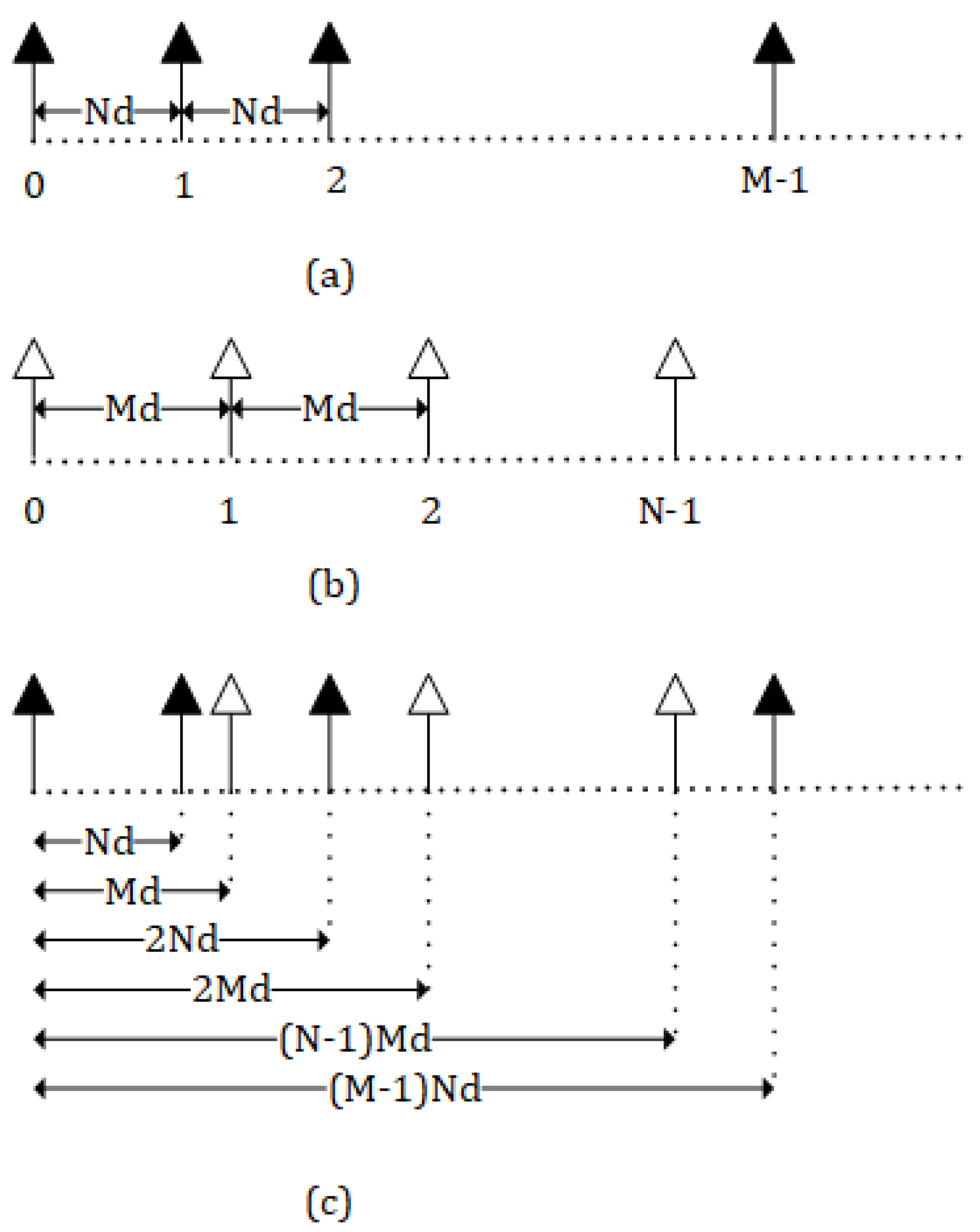
2. Mathematical Modeling

Suppose signals of L narrowband uncorrelated targets are impinging on CSA consisting of two sub ULAs. Sub-array 1 contains M antenna elements having $Nd$ space among each antenna element as shown in Figure 1a while sub-array 2 has N antenna elements $Md$ apart from each other as shown in Figure 1b. M and N are coprime integers and d is equal to the half of the wave length $(\lambda /2)$. By combining these two sub arrays, we get a generalized coprime antenna array having $M+N-1$ elements, as seen in Figure 1c. The first antenna element is shared with both sub-ULAs and physical location of each antenna element of CSA is enclosed in Equation (1).

$$I=\{0,Nd,Md,2Nd,2Md,...,(N-1)Md,(M-1\left)Nd\right\}$$

(1)

Direction of arrival of L uncorrelated signals is summarized in vector $\theta$

$$\theta =[{\theta }_1,{\theta }_2,{\theta }_3,...,{\theta }_L]$$

(2)

Hence, the received signal of L uncorrelated targets impinging on coprime array is given by

$$x\left(t\right)=\sum _{l=1}^L{a}_l\left(\theta \right)s_l\left(t\right)+n\left(t\right)=A\left(\theta \right)s\left(t\right)+n\left(t\right)$$

(3)

where

$$A\left(\theta \right)=[a_1\left(\theta \right),a_2\left(\theta \right),...,a_L\left(\theta \right)]$$

(4)

$$a_l\left(\theta \right)=[1,e^{\pi Nsin{\theta }_l},e^{\pi Msin{\theta }_l},e^{\pi 2Nsin{\theta }_l},e^{\pi 2Msin{\theta }_l},...,e^{\pi (N-1)Mdsin{\theta }_l},e^{\pi (M-1)Ndsin{\theta }_l}]$$

(5)

$$s_l\left(t\right)={[s_1\left(t\right),s_2\left(t\right),...,s_L\left(t\right)]}^T$$

(6)

and $n\left(t\right)$ is the iid and complex additive white Gaussian noise (AWGN) with variance $\sigma I^2$ and zero mean.

$$n\left(t\right)=[n_1\left(t\right),n_2\left(t\right),...n_{M+N-1}\left(t\right)]$$

(7)

Based on this coprime array structure, we can be performed the computation of covariance matrix by taking expectation of the received signal as presented in following equation

$$Rxx=E\left[x\left(t\right)x^H\left(t\right)\right]$$

(8)

By solving this equation we will get

$$Rxx=ARss{A}^H+{\sigma }^{2}I$$

(9)

$Rss$ is the amplitude covariance matrix of received signal as shown in following Equation (9)

$$Rss=E\left[s\left(t\right)s^H\left(t\right)\right]$$

(10)

Now virtual uniform linear array can be obtained by performing vectorization on covariance matrix $\left(Rxx\right)$ as expressed in the following equation

$$z=vec\left(Rxx\right)=vec(ARss{A}^H+{\sigma }^{2}I)=D{\sigma }^2+{\sigma }^{2}I$$

(11)

where D is the Kronecker product and the elements in D are expressed in the form of following equation

$$e^{jK(I_i-I_j)sin{\theta }_{l}wherei,j=0,1,2,...,M+N-1}.$$

(12)

In the process of vectorization, all columns of correlation matrix are placed one by one under the first column. After performing vectorization, the correlation matrix become a column vector $z^{{(M+N-1)}^2\times 1}$. This column vector z is sorted out in accordance with exponent term of the received signal. After sorting, redundant terms of this sorted vector are being skipped. In [33], this can be assessed as continuous virtual uniform linear array (vULA)

$$I_c=\{(Mnd-Nmd)\cup (Nmd-Mnd)\},where0<m<M-1and0<n<N-1$$

(13)

Locations of this vULA elements can be expressed as

$$I_v=\{(I_i-I_j)i,j=0,1,2,...,M+N-1\}$$

(14)

We concentrate on the continuous part of vULA of CSA for application of our proposed algorithms. Due to this continuous part of the vULA, we get a higher degree of freedom and this DOF is directly proportional to the length of continuous vULA.

3. Proposed Methodology

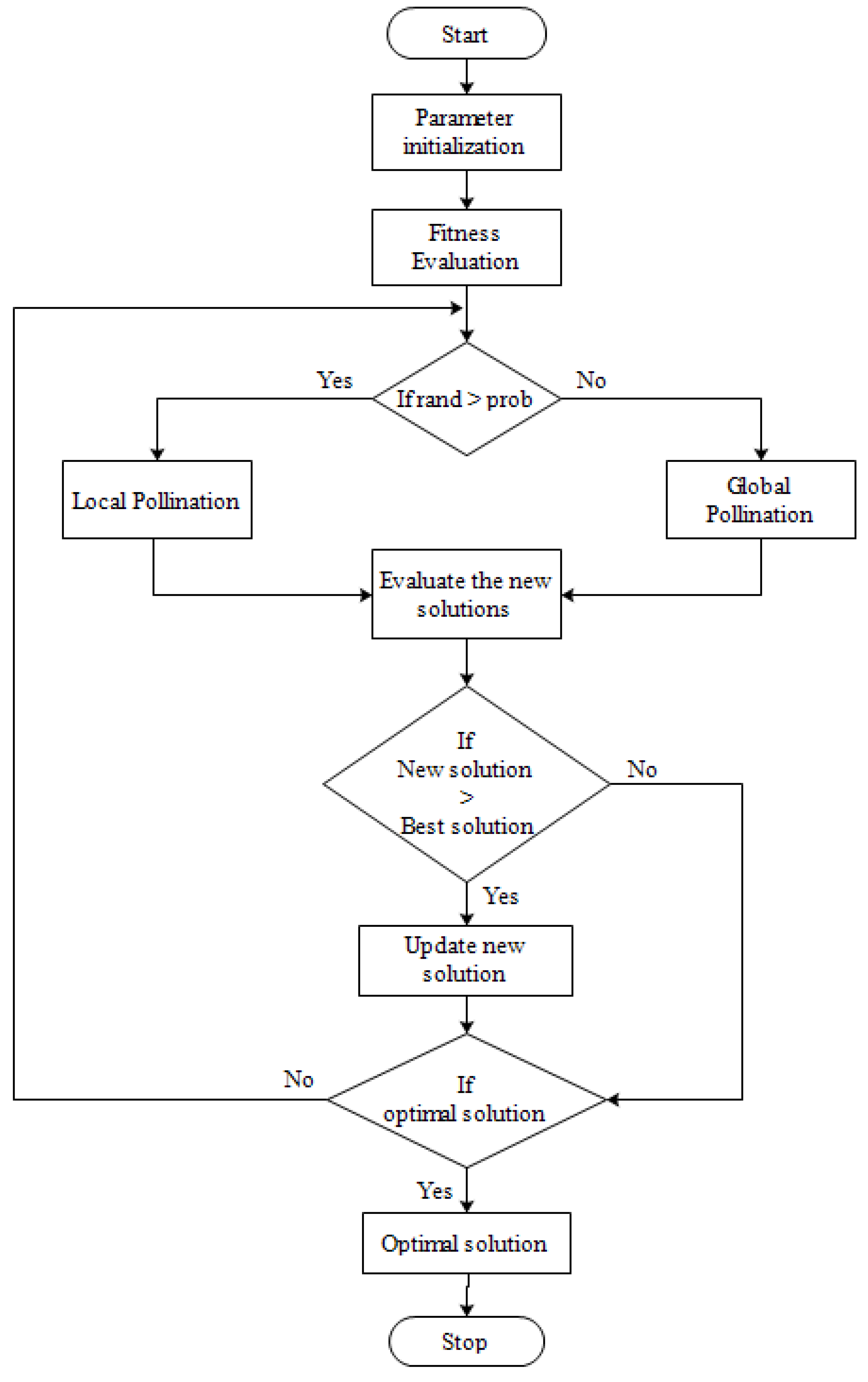
3.1. Flower Pollination Algorithm

In this research article, a flower pollination algorithm is designed to optimize the received signal at coprime antenna arrays. In Figure 2, a flow chart of FPA is illustrated to describe the complete function of FPA. Briefly, the flower pollination algorithm is described in following steps.

Step 1: Population Generation

 

Randomly generate the initial population $x_i$.

Then evaluate the whole population by the help of fitness function $f\left(x_i\right)$.

Step 2: Global pollination process

 

By using Levy distribution, global pollination process is done by executing the following equation

$$x_i^{(t+1)}=x_i^t+L(g^{\ast }-x_i^t)$$

(15)

Step 3: Local pollination process

 

Choose two solutions i and j randomly and generate the parameter $ϵ$ for exploration process by executing following equation

$$x_i^{(t+1)}=x_i^t+ϵ(x_j^t-x_k^t)$$

(16)

Step 4: Update solution

 

At the end we check that if new solution is better than the older one, then set

$$x_i^{t+1}=x_i^{t+1}$$

(17)

otherwise set

$$x_i^{t+1}=x_i^t$$

(18)

This process is repeated until the best solution is achieved.

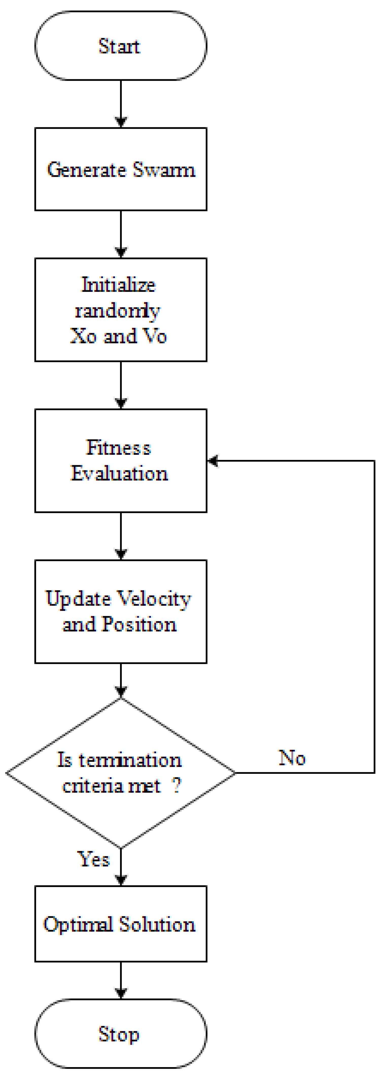
3.2. Particle Swarm Optimization

Particle swarm optimization is a nature inspired robust stochastic optimization technique. The workings of PSO can be explained in following six steps as illustrated in Figure 3

Step 1: Initialization:

 

The PSO algorithm is initialized by a group of random particles and each particle is a solution.

Ater Initializing parameters $\left(x_i\right)$ and velocities $\left(v_i\right)$. Each particle searches for the optimal value by updating the generation.

In each iteration every particle is updated. The first best one is the best solution. After finding the best value particle, update its velocity and position again.

Particle updates its position by

$$x_i^{(t+1)}=x_i^{\left(t\right)}+v_i^{\left(t\right)}\ast t$$

(19)

Particle updates its velocity through following equation

$$x_i^{(t+1)}=w\ast v_i^{\left(t\right)}+c_1\ast v_1(xbest{i}^t-x_i^t)+c_2\ast r_2(gbest{i}^t-x_i^t)$$

(20)

where

$c_1$ is the constant parameter;

$r_1$ is the random parameter;

Xbest is the best particle position;

Gbest is the group best position.

Step 2: Evaluate Fitness:

 

Calculate fitness value for each particle. If fitness value is greater than the gbest then set new value as gbest and choose particle with the best fitness value.

Step 3: For each particle calculate velocity and position from Equations (1) and (2).

 

Step 4: Evaluate Fitness $f\left(x_i^t\right)$ and find current best.

 

Step 5: Update t = t + 1.

 

Step 6: Output gbest and $x_i\left(t\right)$.

 

The process will be continued until the condition is met.

3.3. Fitness Function

Fitness function plays an important role in optimization problems. This is a fundamental tool for the evaluation of the population. This evaluation is performed in each iteration of the algorithm. Fitness function is the difference between the actual and estimated value and it is defined in the following equation

$$f\left(x_i\right)={|x_{a_i}\left(t\right)-x_{e_i}\left(t\right)|}^2$$

(21)

In both methodologies, this fitness function is used for evaluation of pollens and particles.

4. Results, Discussions and Achievements

This section contains various simulated results to validate the potential of FPA and PSO. This analysis is done in term of estimation accuracy, robustness against noise, RMSE vs. snapshots, variation analysis of RMSE, frequency distribution of RMSE, cumulative distribution function of RMSE and box plot analysis under different varying parameters of far field sources. In all of these simulations, Additive White Gaussian Noise (AWGN) channel is assumed with zero mean and variance ${\sigma }^2$ while physical coprime antenna elements are 6 and 200 snapshots are taken for each simulation. All simulated results are compared by estimating seven, nine and eleven targets which are located at $[{20}^0,{40}^0,{60}^0,{80}^0,{100}^0,{120}^0,{140}^0]$,$[{20}^0,{40}^0,{60}^0,{80}^0,{100}^0,{120}^0,{140}^0,{160}^0.{170}^0]$ and $[{20}^0,{35}^0,{50}^0,{65}^0,{80}^0,{95}^0,{110}^0,{120}^0,{135}^0,{150}^0,{165}^0]$ simultaneously.

4.1. Estimation Accuracy

Estimation accuracy of FPA and PSO is looked into by varying the number of sources and their positions. This analysis is set out by best, worst and mean values of the angles estimated by proposed methods to validate their performance along with statistical analysis. In the case of seven targets, we clearly monitored that angles estimated by FPA are accurate than PSO at 0dB, −5 dB and −10 dB SNRs as depicted in

Table 1. Estimation accuracy and STD for seven targets at SNR = 0 dB.

Actual Angles		${\mathit{\theta }}_1=20$	${\mathit{\theta }}_2=40$	${\mathit{\theta }}_3=60$	${\mathit{\theta }}_4=80$	${\mathit{\theta }}_5=100$	${\mathit{\theta }}_6=120$	${\mathit{\theta }}_7=140$
FPA	Best	20.554	39.328	59.914	79.794	100.400	120.194	139.941
	Mean	20.184	36.820	58.325	78.922	102.355	121.292	142.981
	Worst	180.000	37.021	59.478	80.592	100.762	119.896	139.453
	STD	8.0112	7.6306	7.3363	7.2551	7.076	6.7608	13.0759
PSO	Best	22.585	37.755	59.198	79.539	96.225	106.215	120.000
	Mean	23.146	34.461	52.488	63.898	80.206	100.494	119.387
	Worst	0.000	36.178	37.319	58.481	58.711	78.657	98.202
	STD	8.8477	5.3369	10.351	15.299	19.8711	21.992	23.3032

,

Table 2. Estimation accuracy and STD for seven targets at SNR = −5 dB.

Actual Angles		${\mathit{\theta }}_1=20$	${\mathit{\theta }}_2=40$	${\mathit{\theta }}_3=60$	${\mathit{\theta }}_4=80$	${\mathit{\theta }}_5=100$	${\mathit{\theta }}_6=120$	${\mathit{\theta }}_7=140$
FPA	Best	20.554	39.328	59.914	79.794	100.400	120.194	139.941
	Mean	14.697	38.478	59.783	80.211	98.590	121.139	141.271
	Worst	180.000	34.132	60.093	78.950	101.367	119.340	139.785
	STD	8.5051	8.1359	7.6892	7.8932	7.6953	7.3345	13.8623
PSO	Best	24.320	39.690	59.613	79.500	98.327	110.181	120.000
	Mean	24.777	32.753	51.729	63.982	80.608	100.351	119.243
	Worst	0.261	35.533	36.028	55.937	60.200	78.614	98.036
	STD	9.7167	5.8089	11.1897	15.428	19.3838	20.5064	21.6453

and

Table 3. Estimation accuracy and STD for seven targets at SNR = −10 dB.

Actual Angles		${\mathit{\theta }}_1=20$	${\mathit{\theta }}_2=40$	${\mathit{\theta }}_3=60$	${\mathit{\theta }}_4=80$	${\mathit{\theta }}_5=100$	${\mathit{\theta }}_6=120$	${\mathit{\theta }}_7=140$
FPA	Best	21.034	39.874	59.772	80.466	99.778	120.534	139.494
	Mean	25.846	34.286	58.860	76.878	102.507	120.626	144.842
	Worst	179.201	31.046	58.433	76.493	103.240	121.604	145.273
	STD	7.3575	7.0672	5.51	6.1898	5.5168	5.5472	10.4078
PSO	Best	16.144	34.875	57.315	78.143	102.429	120.000	120.000
	Mean	29.010	36.222	52.800	62.549	77.717	101.883	120.000
	Worst	0.000	32.768	33.258	40.144	58.502	78.027	99.566
	STD	12.9084	6.3004	15.559	17.1445	20.1051	19.7943	21.6932

. Furthermore, Table 1, Table 2 and Table 3 includes the standard deviation (STD) analysis for the FPA and PSO models, which clearly define that the proposed model has optimized outcomes.

The statistical analysis including STD for nine targets are declared in

Table 4. Estimation accuracy and STD for nine targets at SNR = 0 dB.

Actual Angles		${\mathit{\theta }}_1=20$	${\mathit{\theta }}_2=40$	${\mathit{\theta }}_3=60$	${\mathit{\theta }}_4=80$	${\mathit{\theta }}_5=100$	${\mathit{\theta }}_6=120$	${\mathit{\theta }}_7=140$	${\mathit{\theta }}_8=160$	${\mathit{\theta }}_9=170$
FPA	Best	21.006	38.750	60.502	79.982	100.441	119.939	140.742	160.451	170.148
	Mean	0.215	39.874	60.583	79.703	100.416	119.783	142.500	179.858	179.915
	Worst	0.000	38.758	58.943	80.572	100.388	120.260	142.292	1.398	0.000
	STD	14.2678	18.1622	14.7291	14.3368	14.2258	13.776	13.9762	13.5198	9.3947
PSO	Best	1.186	37.058	59.335	82.653	96.478	120.000	104.940	75.794	0.000
	Mean	31.074	41.587	55.661	80.701	100.348	118.800	65.155	0.000	0.000
	Worst	38.524	38.120	56.432	79.084	98.278	0.339	0.000	62.001	0.000
	STD	19.9584	39.6766	41.721	38.3223	44.4625	50.1277	56.1085	59.8789	52.0099

,

Table 5. Estimation accuracy and STD for nine targets at SNR = −5 dB.

Actual Angles		${\mathit{\theta }}_1=20$	${\mathit{\theta }}_2=40$	${\mathit{\theta }}_3=60$	${\mathit{\theta }}_4=80$	${\mathit{\theta }}_5=100$	${\mathit{\theta }}_6=120$	${\mathit{\theta }}_7=140$	${\mathit{\theta }}_8=160$	${\mathit{\theta }}_9=170$
FPA	Best	20.063	40.167	59.702	79.861	100.205	120.889	140.965	162.774	171.189
	Mean	23.035	34.792	57.209	80.132	100.174	116.792	129.355	154.086	156.307
	Worst	11.371	36.931	59.788	78.922	99.862	120.054	134.764	151.199	0.250
	STD	10.8943	14.1462	13.4699	13.8556	14.1729	13.4184	13.5677	13.3974	9.9573
PSO	Best	0.885	36.881	59.177	79.224	97.356	120.000	120.000	105.922	0.000
	Mean	31.074	41.587	55.661	80.701	100.348	118.800	65.155	0.000	0.000
	Worst	38.524	38.120	56.432	79.084	98.278	0.339	0.000	62.001	0.000
	STD	19.9206	39.5109	31.5467	36.5097	42.1808	48.2541	54.0918	57.903	50.7356

and

Table 6. Estimation accuracy and STD for nine targets at SNR = −10 dB.

Actual Angles		${\mathit{\theta }}_1=20$	${\mathit{\theta }}_2=40$	${\mathit{\theta }}_3=60$	${\mathit{\theta }}_4=80$	${\mathit{\theta }}_5=100$	${\mathit{\theta }}_6=120$	${\mathit{\theta }}_7=140$	${\mathit{\theta }}_8=160$	${\mathit{\theta }}_9=170$
FPA	Best	18.168	38.385	59.174	79.491	101.673	119.234	140.863	158.025	170.230
	Mean	0.000	32.733	58.255	77.206	101.260	117.178	127.036	148.510	169.016
	Worst	11.230	38.897	61.967	79.402	100.536	119.506	143.753	2.138	0.000
	STD	11.5865	15.2439	15.913	15.1088	15.3368	13.0878	13.8784	12.2759	11.0899
PSO	Best	0.371	36.758	59.827	79.031	97.880	120.000	120.000	106.209	0.000
	Mean	29.041	41.913	59.563	80.782	102.079	119.840	73.947	0.000	0.000
	Worst	37.783	37.524	59.243	78.662	99.615	58.886	0.000	0.000	0.000
	STD	19.9239	39.508	40.2039	36.9535	42.1866	48.3715	55.2631	58.0799	51.2382

, comparing the performance of FPA and PSO algorithms. The outcomes prove that the computation analysis of FPA is more optimized than PSO.

Table 7. Estimation accuracy and STD for eleven targets at SNR = 0 dB.

Actual Angles		${\mathit{\theta }}_1=20$	${\mathit{\theta }}_2=35$	${\mathit{\theta }}_3=50$	${\mathit{\theta }}_4=65$	${\mathit{\theta }}_5=80$	${\mathit{\theta }}_6=95$	${\mathit{\theta }}_7=110$	${\mathit{\theta }}_8=120$	${\mathit{\theta }}_9=135$	${\mathit{\theta }}_{10}=150$	${\mathit{\theta }}_{11}=165$
FPA	Best	20.399	34.092	50.469	66.942	80.878	95.569	109.970	118.790	134.319	150.301	160.555
	Mean	17.832	20.145	40.542	55.367	73.083	89.377	104.883	115.665	124.661	145.335	149.661
	Worst	2.486	28.774	44.332	58.798	74.446	89.797	103.624	118.702	136.652	148.535	0.257
	STD	12.8879	13.0721	9.6502	10.2882	10.2654	10.3802	10.0996	8.9518	9.696	9.9422	12.3896
PSO	Best	33.810	45.343	60.019	73.433	82.736	92.641	112.055	120.000	101.111	0.000	0.000
	Mean	1.489	32.933	54.975	65.939	75.908	97.667	110.797	119.215	85.444	42.657	0.000
	Worst	0.653	38.887	39.501	63.090	83.131	74.659	96.677	114.281	55.525	0.489	0.276
	STD	19.8683	34.3679	23.1016	23.4132	27.2577	30.5871	34.19	33.4794	37.3056	39.7499	45.8505

,

Table 8. Estimation accuracy and STD for eleven targets at SNR = −5 dB.

Actual Angles		${\mathit{\theta }}_1=20$	${\mathit{\theta }}_2=35$	${\mathit{\theta }}_3=50$	${\mathit{\theta }}_4=65$	${\mathit{\theta }}_5=80$	${\mathit{\theta }}_6=95$	${\mathit{\theta }}_7=110$	${\mathit{\theta }}_8=120$	${\mathit{\theta }}_9=135$	${\mathit{\theta }}_{10}=150$	${\mathit{\theta }}_{11}=165$
FPA	Best	23.21	34.09	51.73	66.56	80.511	94.689	109.868	121.81	136.79	150.969	165.004
	Mean	2.178	31.737	48.094	67.517	83.290	98.378	112.733	121.49	137.75	143.524	180
	Worst	2.998	34.678	40.895	60.643	76.488	93.857	107.342	115.7	127.69	143.557	0.603
	STD	11.2746	10.9455	9.9859	9.763	9.5543	9.17	7.709	6.8242	8.9132	10.3684	11.8853
PSO	Best	0.000	32.31	41.51	68.749	80.010	94.0313	106.08	120	114.28	57.657	0.977
	Mean	0.601	32.904	55.206	66.032	77.191	90.0479	112.28	119.11	101.44	40.682	0.703
	Worst	38.766	38.310	57.192	64.507	82.03	96.142	114.12	73.873	2.232	1.491	0.000
	STD	19.7599	34.0793	18.3588	25.726	25.3566	29.5459	33.0406	29.977	33.9386	37.9637	45.2615

and

Table 9. Estimation accuracy and STD for eleven targets at SNR = −10 dB.

Actual Angles		${\mathit{\theta }}_1=20$	${\mathit{\theta }}_2=35$	${\mathit{\theta }}_3=50$	${\mathit{\theta }}_4=65$	${\mathit{\theta }}_5=80$	${\mathit{\theta }}_6=95$	${\mathit{\theta }}_7=110$	${\mathit{\theta }}_8=120$	${\mathit{\theta }}_9=135$	${\mathit{\theta }}_{10}=150$	${\mathit{\theta }}_{11}=165$
FPA	Best	19.25	36.78	51.86	64.31	79.67	96.18	110.49	120.45	135.79	153.02	166.20
	Mean	28.37	34.49	55.83	72.93	88.82	104.98	116.67	125.51	144.95	153.74	179.04
	Worst	29.76	37.34	55.15	72.85	89.77	106.00	0.25	121.24	143.21	146.09	0.000
	STD	12.1514	11.0382	10.2101	10.6042	11.3763	11.875	7.0773	7.7574	9.3693	10.463	11.8565
PSO	Best	0.00	30.76	40.60	65.41	83.42	95.62	106.44	120	114.23	74.80	55.77
	Mean	0.00	34.07	39.52	64.19	84.78	99.33	111.87	117.29	73.77	53.86	0.00
	Worst	38.82	38.12	38.20	60.94	75.77	58.90	111.06	117.28	0.13	0.26	0.41
	STD	19.7866	33.973	21.9043	25.7832	28.1443	31.7251	36.0186	33.9977	34.4507	38.2707	46.2669

illustrate the analysis of different angles in terms of best, mean, worst and STD for FPA and PSO algorithms. By keeping in view the analysis of STD, it clearly observed that the achievements of FPA are much better than PSO.

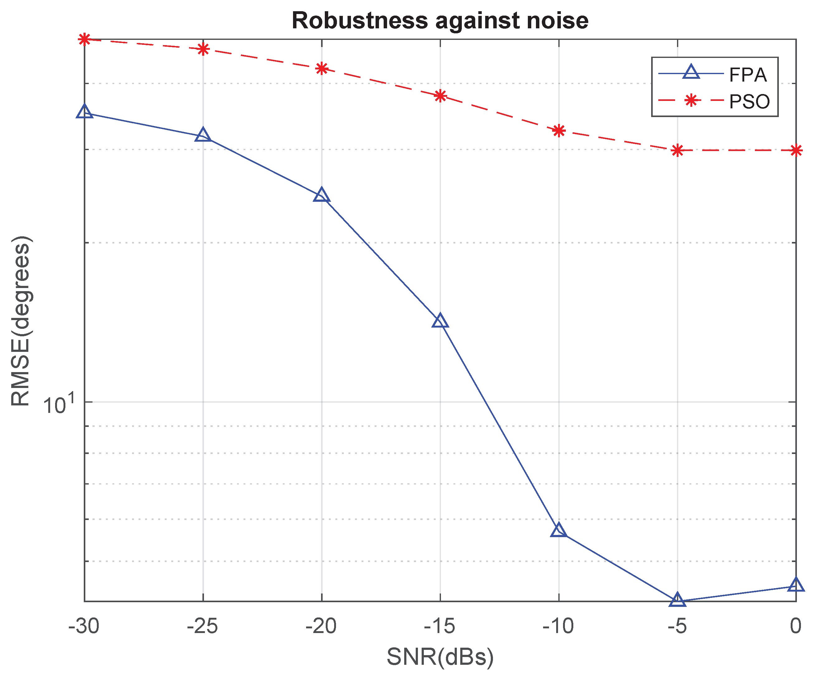
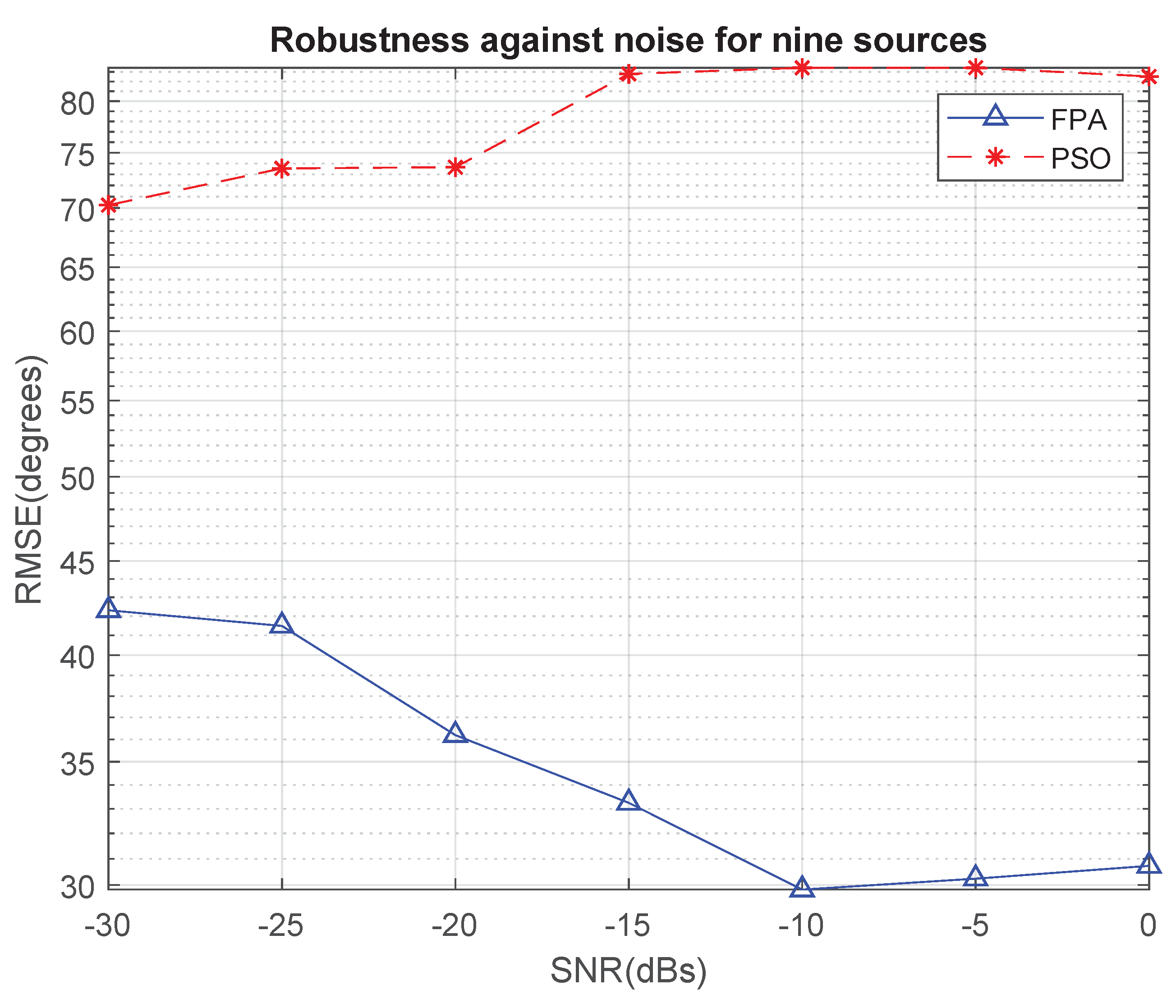
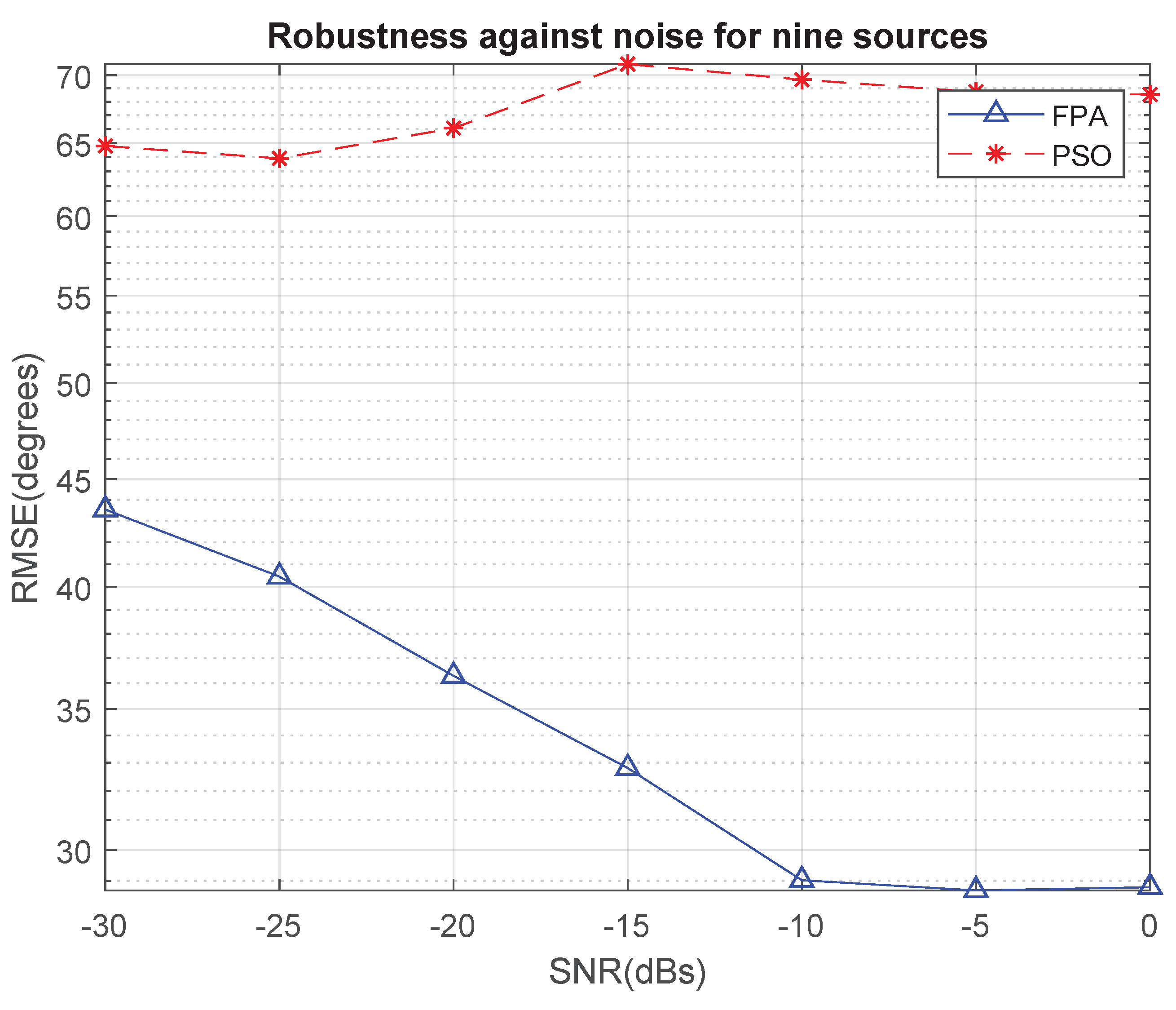
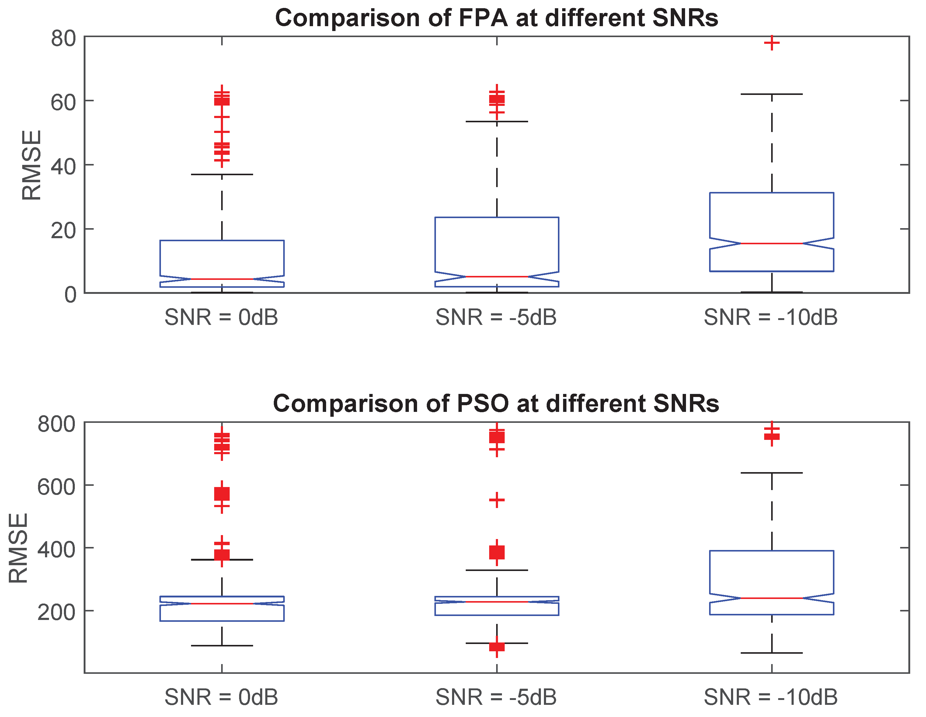
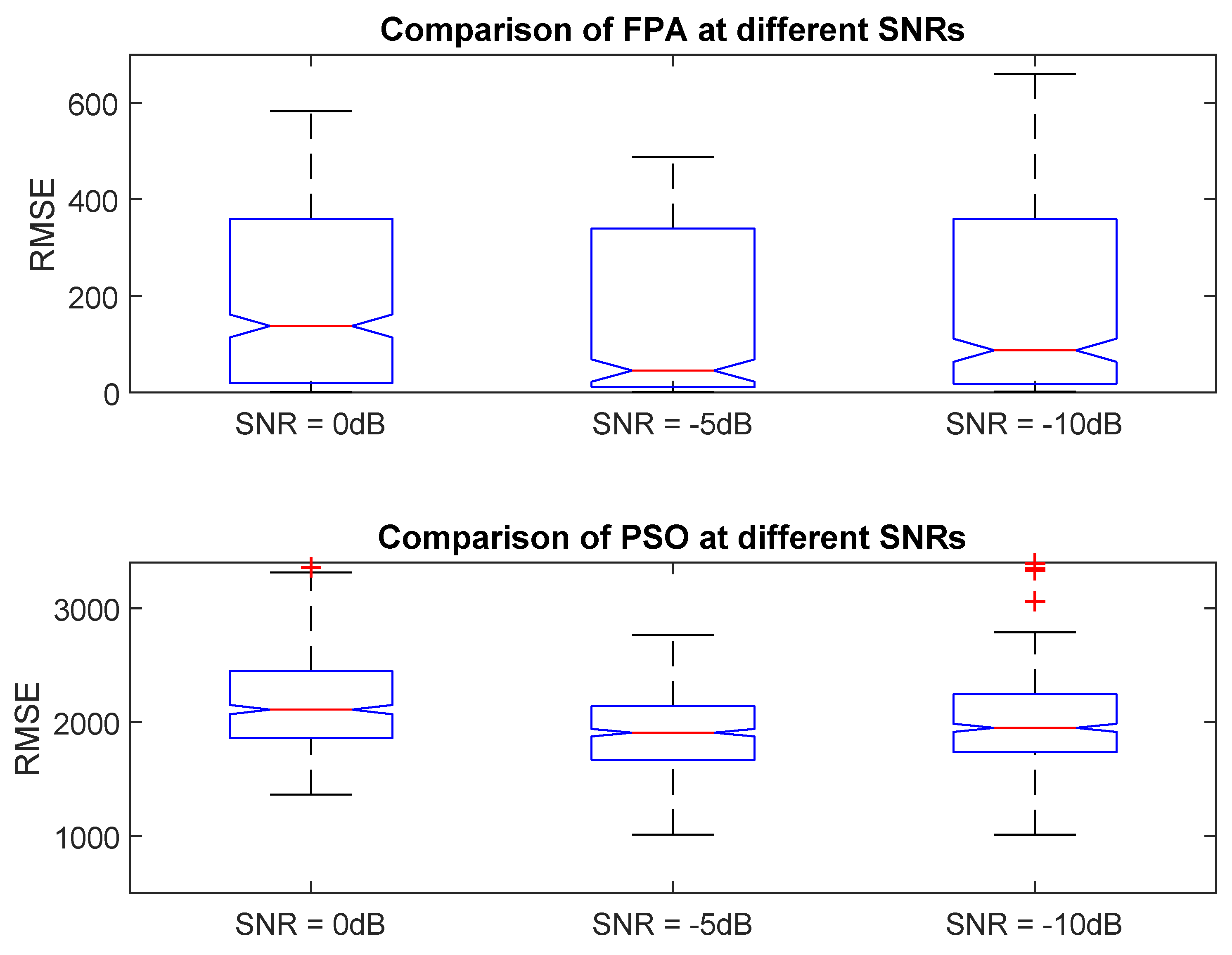
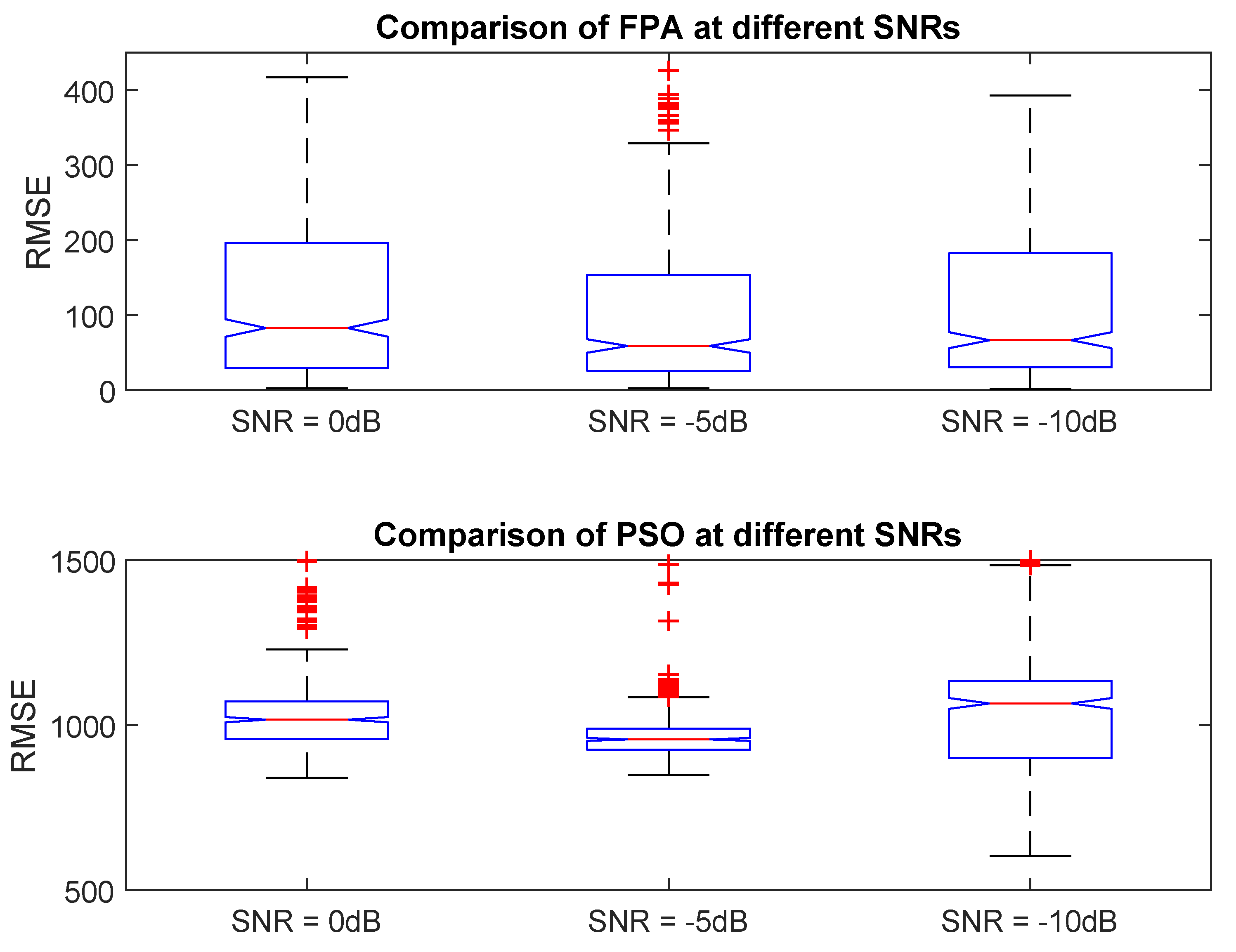
4.2. Robustness against Noise

Robustness against noise is one of the best analysis to measure the performance of algorithms used for DOA estimation. In this analysis, as signal to noise ratio increases, the value of RMSE decreases. RMSE is the performance indicator against different numbers of SNR in this analysis. In all three cases, FPA shows much robustness against noise than PSO as shown in Figure 4, Figure 5 and Figure 6.

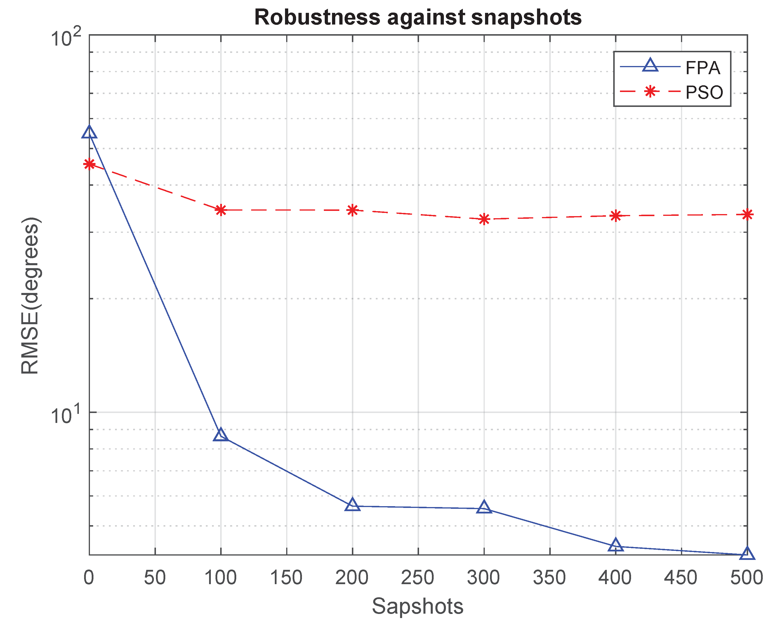
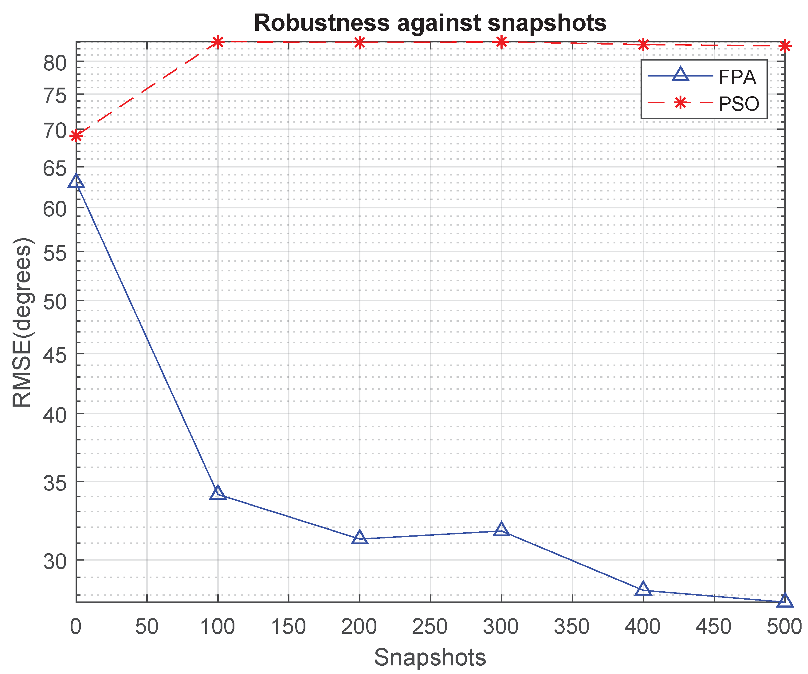
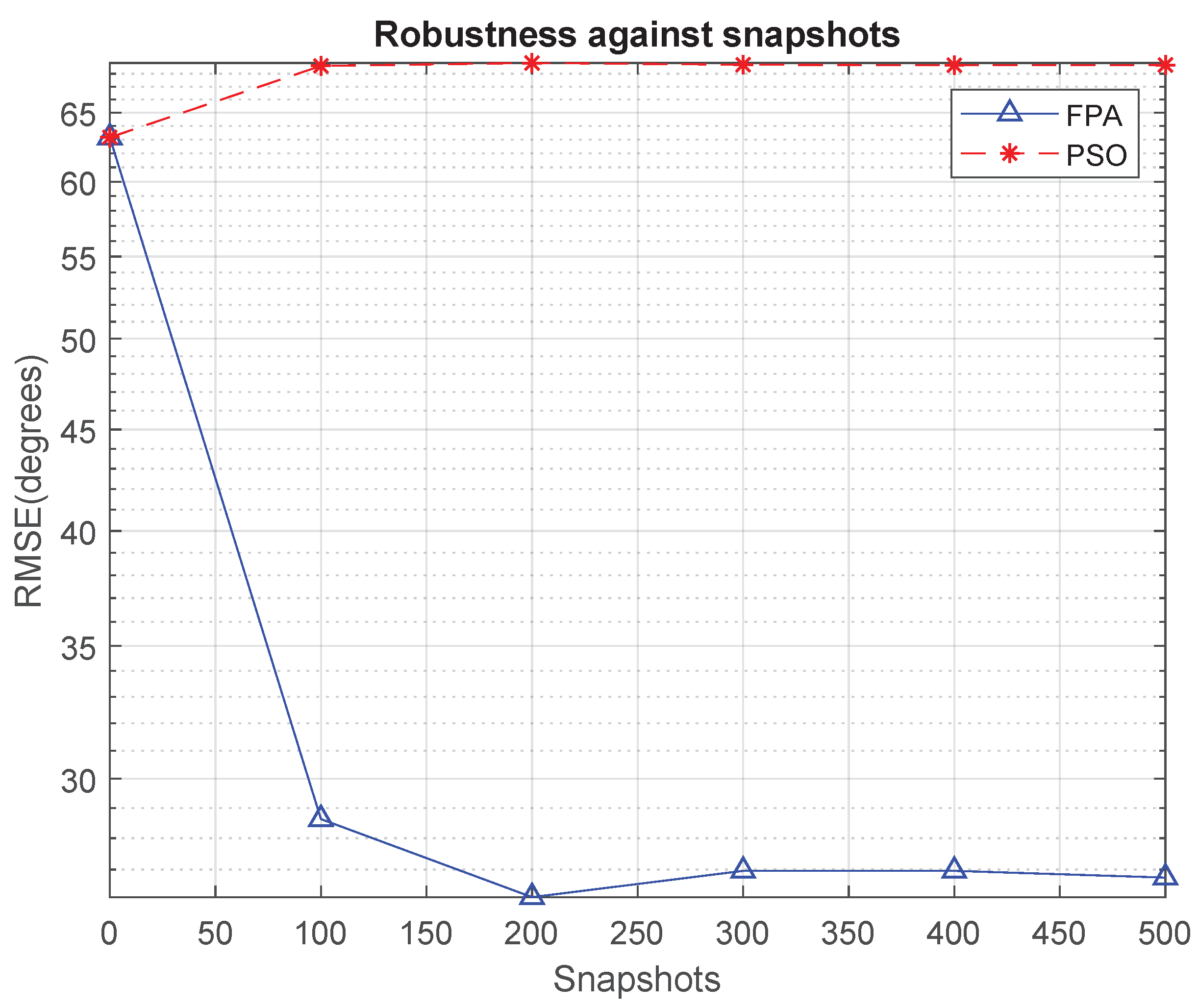
4.3. RMSE Analysis against Multiple Snapshots

Based on Figure 4, Figure 5 and Figure 6, the value of Root Mean Square Error (RMSE) is observed by increasing the Signal to Noise Ratio (SNR) from −30 dB to 0 dB while in Figure 7, Figure 8 and Figure 9 comparison of RMSE for FPA and PSO is performed with respect to a number of snapshots. In array signal processing, when direction of arrival estimation is performed multiple snapshots of the received signal are taken while we simulate the problem. If value of error reduced gradually when increasing the number of snapshots, it means that our algorithm works properly. Therefore, we perform the comparison of RMSE vs. snapshots for FPA and PSO in Figure 7, Figure 8 and Figure 9 to explore the superiority of the algorithms. It can be clearly observed in Figure 7, Figure 8 and Figure 9, that FPA is more effective for DOA estimation with enhanced degree of freedom than PSO. Moreover, as number of snapshots increases, RMSE decreases gradually.

4.4. Variation Analysis of RMSE

A box-plot is a standard way to demonstrate the distribution of error in accordance with $Q_1$,$Q_2$,$Q_3$, min and max value of data. We distinguish the min and max values on the basis of outlier and in conformity with outlier, we easily identify the performance of the proposed methodologies. In Figure 10 maximum RMSE of FPA is 40, 55 and 60 at 0 dB, −5 dB and −10 dB, respectively. Whereas at 0 dB, −5 dB and −10 dB the relative maximum RMSE is below 400 and 600. These plots showed that FPA performed vastly superior than PSO.

In the case of nine targets, it can be easily observed that spread of RMSE of FPA is far less than PSO at 0dB, −5 dB and −10 dB as depicted in Figure 11. In the case of eleven targets detection, again the performance of FPA is outclassed, as illustrated in Figure 12. In accordance with this diagram RMSE spread of FPA is below 200 at 0 dB, −5 dB and −10 dB while this spread is more than 1300 in case of PSO.

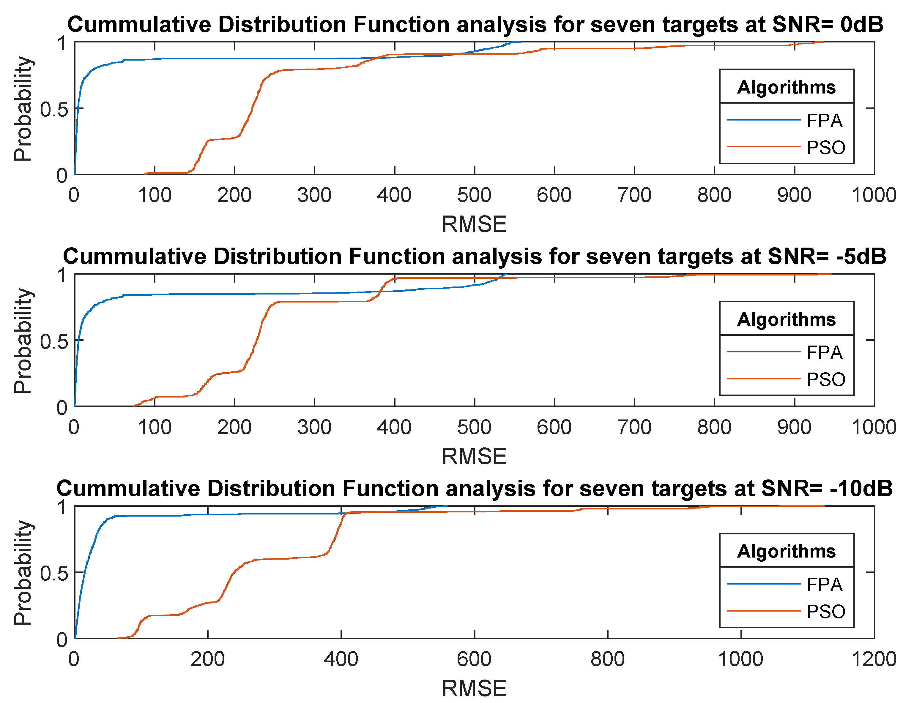
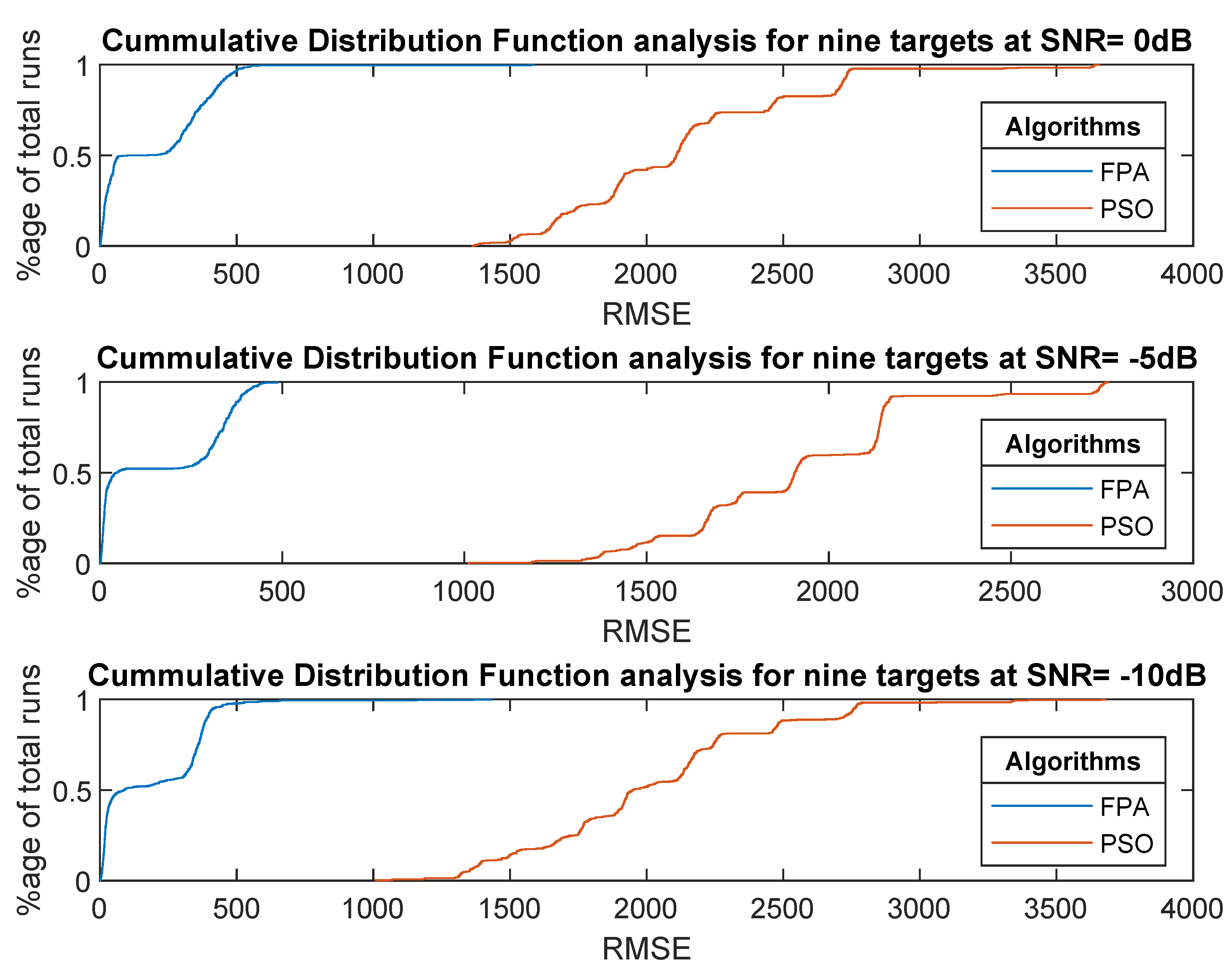
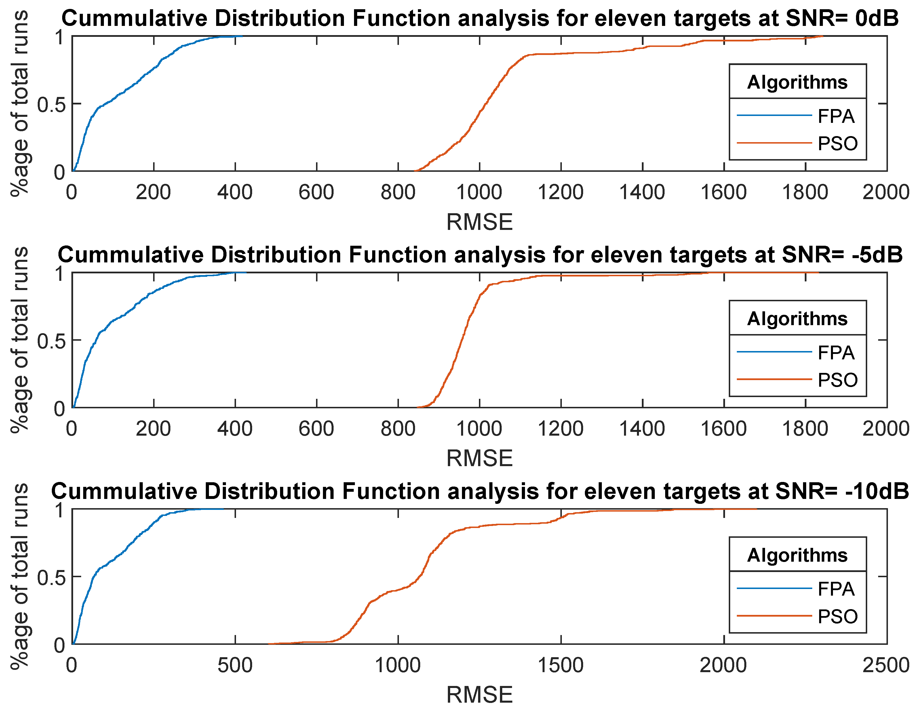
4.5. Cumulative Distribution Function of RMSE

CDF is a non decreasing function and in this subsection, it is applied to specify the persistence and failure times of optimization techniques in respect with Monte Carlo runs. CDF is the part of probability density function and it is presented in the form of probability. Figure 13 shows that FPA performs very well as compared to PSO in respect with RMSE. In case of FPA, RMSE has been occurred around zero at 80% of MC runs at 0 dB, −5 dB and −10 dB while RMSE is exceeded up to 150 at 25% of MC runs of PSO algorithm.

In case of nine targets estimation, again FPA performs superbly. The value of RMSE is near to zero at 50% of MC runs while it exceed up to 1500 in the scenario of PSO at 0 dB, −5 dB and −10 dB as depicted in Figure 14.

In case of eleven targets estimation, the performance of FPA is remarkable. In this case, the RMSE value is near to 50 at 50% of MC runs in FPA algorithm while it exceed 1000 in the scenario of PSO at 0 dB, −5 dB and −10 dB as shown in Figure 15.

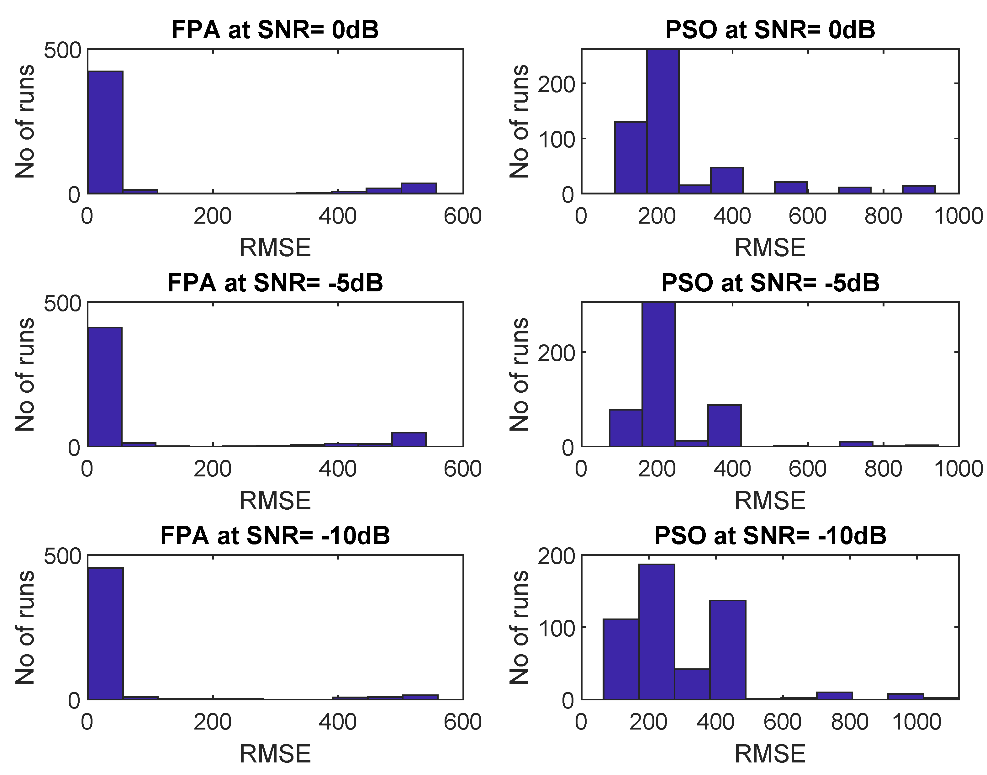
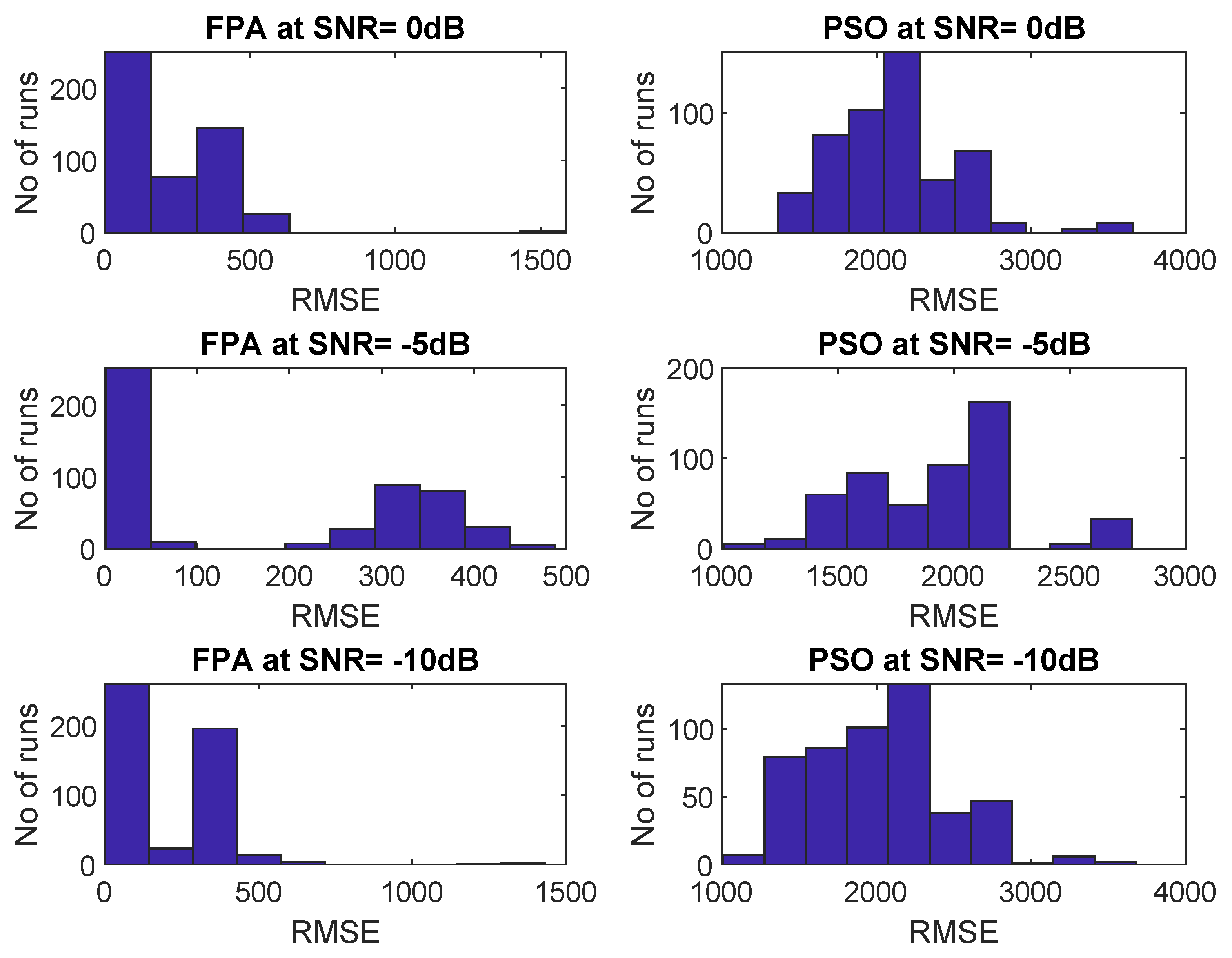
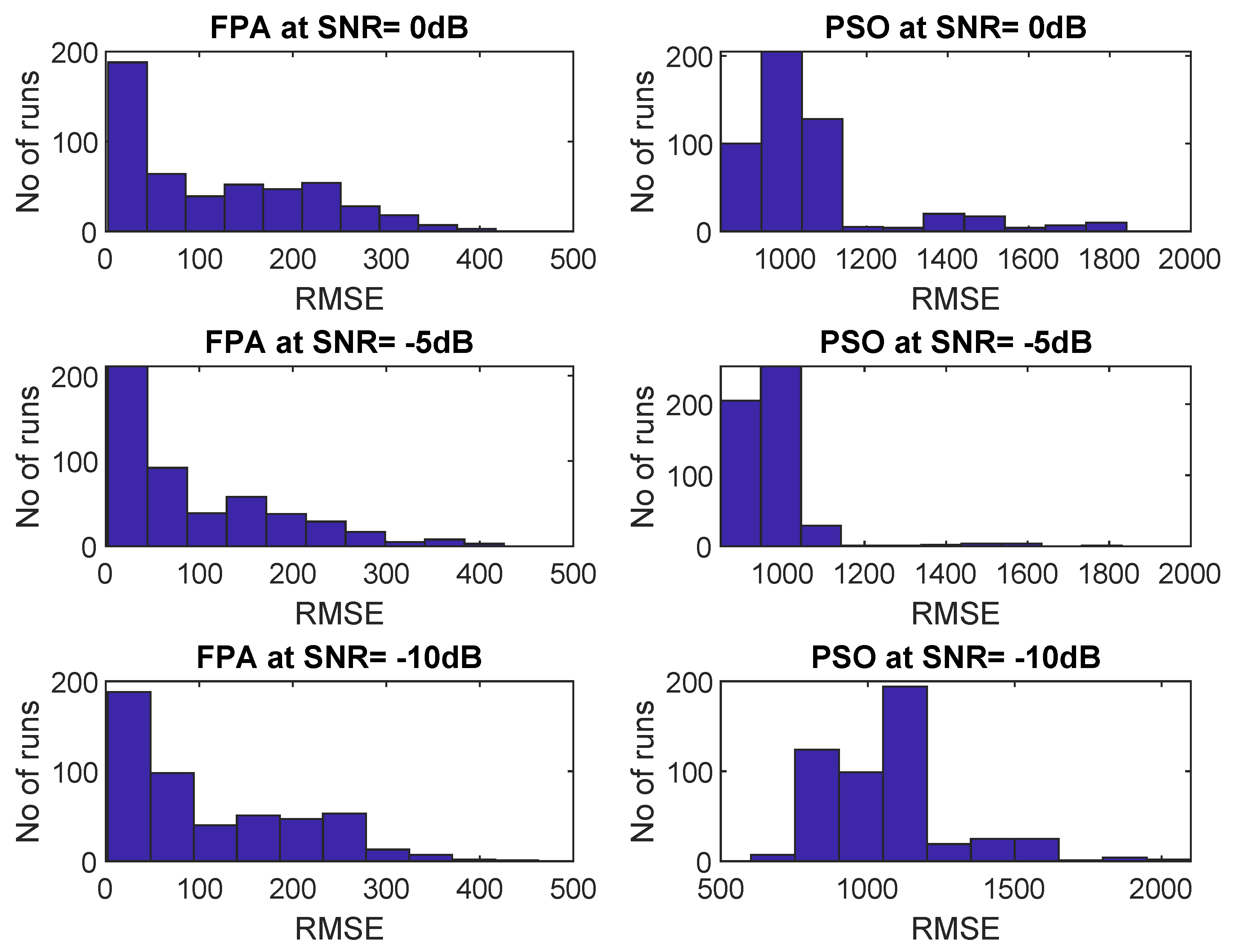
4.6. Histogram Analysis of RMSE

In histogram representation, bars are in the form of continuous grouping. In this analysis, we check how much RMSE occurred against Monte Carlo runs. On the basis of this analysis, we checked the performance of algorithms. In Figure 16 RMSE of FPA is very low at 0dB, −5 dB and −10 dB SNR over 500 iterations. In the same scenario, RMSE of PSO increases gradually as SNR decreases. Thus, we clearly observed that FPA performed very well as compared to PSO on the basis of RMSE distribution.

In Figure 17, RMSE spread of FPA is very low at 0dB, −5 dB and −10 dB SNR in accordance with 500 iterations while spread of RMSE of PSO is very wide. Thus, it can be noticed clearly that performance of is much better as compared to PSO on the basis of RMSE distribution.

As per Figure 18, RMSE spread of FPA is very small at 0 dB, −5 dB and −10 dB SNR with respect to 500 iterations while RMSE spread of PSO more wider. Thus, it can be examine easily that performance of FPA is much better as compared to PSO on the basis of RMSE distribution.

5. Conclusions

In this paper, we estimate DOA of electromagnetic waves received at coprime arrays through the Flower Pollination Algorithm. In DOA estimation, enhanced degree of freedom and estimation accuracy are the main challenges in a low SNR environment. Deterministic algorithms provide high resolution, but performance of these algorithms is degraded when we need higher DOF in a low SNR regime. However, meta heuristic algorithm, as we implement FPA in this paper, provides higher DOF and resolution ability at low SNR. In the future, we will expand the span of this study by estimating other parameters like frequency and amplitude of the impinging waves by exploring advance meta heuristic techniques.

References

1. Zhang, Y.; Hu, G.; Zhu, M.; Zhan, C.; Zhao, F.; Zhou, H.; Zhao, F.; Yue, S. DOA estimation based on average processing of redundant virtual array elements for coprime MIMO RADAR. J. Phys. Conf. Ser. 2021, 1894, 012092. [Google Scholar] [CrossRef]
2. Wen, F.; Mao, C.; Zhang, G. Direction finding in MIMO RADAR with large antenna arrays and non-orthogonal waveforms. Digit. Signal Process. 2019, 94, 75–83. [Google Scholar] [CrossRef]
3. Jing, H.; Wang, H.; Liu, Z.; Shen, X. DOA estimation for underwater target by active detection on virtual time reversal using a uniform linear array. Sensors 2018, 18, 2458. [Google Scholar] [CrossRef] [Green Version]
4. Straser, V.; Cataldi, D.; Cataldi, G. Radio direction finding system, a new perspective for global crust diagnosis. New Concepts Glob. Tectonics J. 2018, 6, 203–211. [Google Scholar]
5. Wang, J.J.-M.; Liu, J.; Pare, T.E., Jr.; Wu, T.; Bajko, G.; Hsu, Y.-P. Direction Finding and Ftm Positioning in Wireless Local Area Networks. U.S. Patent 10,484,814, 19 November 2019. [Google Scholar]
6. Suryavanshi, N.B.; Reddy, K.V.; Chandrika, V.R. Direction finding capability in bluetooth 5.1 standard. In International Conference on Ubiquitous Communications and Network Computing; Springer: Berlin/Heidelberg, Germany, 2019; pp. 53–65. [Google Scholar]
7. Qin, S.; Zhang, Y.D.; Amin, M.G.; Himed, B. DOA estimation exploiting a uniform linear array with multiple co-prime frequencies. Signal Process. 2017, 130, 37–46. [Google Scholar] [CrossRef] [Green Version]
8. Guo, M.; Zhang, Y.D.; Chen, T. DOA estimation using compressed sparse array. IEEE Trans. Signal Process. 2018, 66, 4133–4146. [Google Scholar] [CrossRef]
9. Elbir, A.M. Two-dimensional DOA estimation via shifted sparse arrays with higher degrees of freedom. Circuits Syst. Signal Process. 2019, 38, 5549–5575. [Google Scholar] [CrossRef]
10. Liu, K.; Zhang, Y.D. Coprime array-based DOA estimation in unknown nonuniform noise environment. Digit. Signal Process. 2018, 79, 66–74. [Google Scholar] [CrossRef]
11. Chen, C.-Y.; Vaidyanathan, P.P. Minimum redundancy mimo radars. In Proceedings of the 2008 IEEE International Symposium on Circuits and Systems, Seattle, WA, USA, 18–21 May 2008; pp. 45–48. [Google Scholar]
12. Pal, P.; Vaidyanathan, P.P. Nested arrays: A novel approach to array processing with enhanced degrees of freedom. IEEE Trans. Signal Process. 2010, 58, 4167–4181. [Google Scholar] [CrossRef] [Green Version]
13. Liu, J.; Zhang, Y.; Lu, Y.; Ren, S.; Cao, S. Augmented nested arrays with enhanced DOF and reduced mutual coupling. IEEE Trans. Signal Process. 2017, 65, 5549–5563. [Google Scholar] [CrossRef]
14. Vaidyanathan, P.P.; Pal, P. Sparse sensing with coprime arrays. In Proceedings of the 2010 Conference Record of the forty Fourth Asilomar Conference on Signals, Systems and Computers, Pacific Grove, CA, USA, 7–10 November 2010; pp. 1405–1409. [Google Scholar]
15. Zheng, Z.; Huang, Y.; Wang, W.; So, H.C. Direction-of-arrival estimation of coherent signals via coprime array interpolation. IEEE Signal Process. Lett. 2020, 27, 585–589. [Google Scholar] [CrossRef]
16. Adhikari, K.; Drozdenko, B. Symmetry-imposed rectangular coprime and nested arrays for direction of arrival estimation with multiple signal classification. IEEE Access 2019, 7, 153217–153229. [Google Scholar] [CrossRef]
17. Muhammad, M.; Li, M.; Abbasi, Q.H.; Goh, C.; Imran, M. Direction of arrival estimation using hybrid spatial cross-cumulants and root-music. In Proceedings of the 2020 14th European Conference on Antennas and Propagation (EuCAP), Copenhagen, Denmark, 15–20 March 2020; pp. 1–5. [Google Scholar]
18. Ning, Y.; Ma, S.; Meng, F.; Wu, Q. DOA estimation based on ESPRIT algorithm method for frequency scanning LWA. IEEE Commun. Lett. 2020, 24, 1441–1445. [Google Scholar] [CrossRef]
19. Hakam, A.; Shubair, R.M.; Salahat, E. Enhanced DOA estimation algorithms using MVDR and MUSIC. In Proceedings of the 2013 International Conference on Current Trends in Information Technology (CTIT), Dubai, United Arab Emirates, 11–12 December 2013; pp. 172–176. [Google Scholar]
20. Wang, P.; Kong, Y.; He, X.; Zhang, M.; Tan, X. An improved squirrel search algorithm for maximum likelihood DOA estimation and application for MEMS vector hydrophone array. IEEE Access 2019, 7, 118343–118358. [Google Scholar] [CrossRef]
21. Jaafer, Z.; Goli, S.; Elameer, A.S. Best performance analysis of DOA estimation algorithms. In Proceedings of the 2018 1st Annual International Conference on Information and Sciences (AiCIS), Fallujah, Iraq, 20–21 November 2018; pp. 235–239. [Google Scholar]
22. Vikas, B.; Vakula, D. Performance comparision of MUSIC and ESPRIT algorithms in presence of coherent signals for DOA estimation. In Proceedings of the 2017 International conference of Electronics, Communication and Aerospace Technology (ICECA), Coimbatore, India, 20–22 April 2017; Volume 2, pp. 403–405. [Google Scholar]
23. Ahmed, N.; Wang, H.; Raja, M.A.Z.; Ali, W.; Zaman, F.; Khan, W.U.; He, Y. Performance analysis of efficient computing techniques for direction of arrival estimation of underwater multi targets. IEEE Access 2021, 9, 33284–33298. [Google Scholar] [CrossRef]
24. Yang, X.-S. Flower pollination algorithm for global optimization. In International Conference on Unconventional Computing and Natural Computation; Springer: Berlin/Heidelberg, Germany, 2012; pp. 240–249. [Google Scholar]
25. Qamar, M.S.; Tu, S.; Ali, F.; Armghan, A.; Munir, M.F.; Alenezi, F.; Muhammad, F.; Ali, A.; Alnaim, N. Improvement of Traveling Salesman Problem Solution Using Hybrid Algorithm Based on Best-Worst Ant System and Particle Swarm Optimization. Appl. Sci. 2021, 11, 4780. [Google Scholar] [CrossRef]
26. Hammed, K.; Ghauri, S.A.; Qamar, M.S. Biological inspired stochastic optimization technique (pso) for DOA and amplitude estimation of antenna arrays signal processing in RADAR communication system. J. Sens. 2016, 2016. [Google Scholar] [CrossRef] [Green Version]
27. Zhao, H.; Hou, Y.; Mao, X. A synthetic layout method for distributed Nested Circular Array based on Ant colony algorithm. In Proceedings of the IET International RADAR Conference (IET IRC 2020), Chongqing, China, 4–6 November 2020; pp. 955–959. [Google Scholar]
28. Parsa, S.A.H.; Zadeh, A.E.; Kazemitabar, S.J. A novel modified artificial bee colony for doa estimation. Int. J. Sens. Wirel. Commun. Control 2021, 11, 96–106. [Google Scholar] [CrossRef]
29. Jia, W.; Liu, S. Application of Simulated Annealing Genetic Algorithm in DOA estimation technique. Comput. Eng. Appl. 2014, 12, 266–270. [Google Scholar]
30. Das, S.; Suganthan, P.N. Differential Evolution: A survey of the state-of-the-art. IEEE Trans. Evol. Comput. 2010, 15, 4–31. [Google Scholar] [CrossRef]
31. Chen, H.; Li, H.; Yang, M.; Xiang, C.; Suzuki, M. General Improvements of Heuristic Algorithms for Low Complexity DOA Estimation. Int. J. Antennas Propag. 2019, 2019, 3858794. [Google Scholar] [CrossRef]
32. Sallam, T.A.R.; Abdel-Rahman, A.B.; Alghoniemy, M.; Kawasaki, Z. Flower Pollination Algorithm for Adaptive Beamforming of Phased Array Antennas. J. Mach. Intell. 2017, 2, 1–5. [Google Scholar] [CrossRef]
33. Pal, P.; Vaidyanathan, P.P. Coprime sampling and the MUSIC algorithm. In Proceedings of the 2011 Digital Signal Processing and Signal Processing Education Meeting (DSP/SPE), Sedona, AZ, USA, 4–7 January 2011; IEEE: Piscataway, NJ, USA, 2011; pp. 289–294. [Google Scholar]
Figure 1. Coprime antenna array configuration: (a) sub antenna array 1; (b) sub antenna array 2; (c) generalize coprime antenna array.
Applsci 11 07985 g001
Figure 2. Flow diagram for Flower Pollination Algorithm.
Applsci 11 07985 g002
Figure 3. Flow diagram for Particle Swarm Optimization.
Applsci 11 07985 g003
Figure 4. Robustness against noise for seven targets.
Applsci 11 07985 g004
Figure 5. Robustness against noise for nine targets.
Applsci 11 07985 g005
Figure 6. Robustness against noise for eleven targets.
Applsci 11 07985 g006
Figure 7. Robustness against snapshots for seven targets.
Applsci 11 07985 g007
Figure 8. Robustness against snapshots for nine targets.
Applsci 11 07985 g008
Figure 9. Robustness against snapshots for eleven targets.
Applsci 11 07985 g009
Figure 10. Variation analysis of RMSE for seven targets.
Applsci 11 07985 g010
Figure 11. Variation analysis of RMSE for nine targets.
Applsci 11 07985 g011
Figure 12. Variation analysis of RMSE for eleven targets.
Applsci 11 07985 g012
Figure 13. CDF analysis of RMSE for seven targets at different SNRs.
Applsci 11 07985 g013
Figure 14. CDF analysis of RMSE for nine targets at different SNRs.
Applsci 11 07985 g014
Figure 15. CDF analysis of RMSE for eleven targets at different SNRs.
Applsci 11 07985 g015
Figure 16. Histogram analysis of RMSE for seven targets.
Applsci 11 07985 g016
Figure 17. Histogram analysis of RMSE for nine targets.
Applsci 11 07985 g017
Figure 18. Histogram analysis of RMSE for eleven targets.
Applsci 11 07985 g018