Repetitive Learning Sliding Mode Stabilization Control for a Flexible-Base, Flexible-Link and Flexible-Joint Space Robot Capturing a Satellite

Abstract

During the process of satellite capture by a flexible base–link–joint space robot, the base, joints, and links vibrate easily and also rotate in a disorderly manner owing to the impact torque. To address this problem, a repetitive learning sliding mode stabilization control is proposed to stabilize the system. First, the dynamic models of the fully flexible space robot and the captured satellite are established, respectively, and the impact effect is calculated according to the motion and force transfer relationships. Based on this, a dynamic model of the system after capturing is established. Subsequently, the system is decomposed into slow and fast subsystems using the singular perturbation theory. To ensure that the base attitude and the joints of the slow subsystem reach the desired trajectories, link vibrations are suppressed simultaneously, and a repetitive learning sliding mode controller based on the concept of the virtual force is designed. Moreover, a multilinear optimal controller is proposed for the fast subsystem to suppress the vibration of the base and joints. Two sub-controllers constitute the repetitive learning sliding mode stabilization control for the system. This ensures that the base attitude and joints of the system reach the desired trajectories in a limited time after capturing, obtain better control quality, and suppress the multiple flexible vibrations of the base, links and joints. Finally, the simulation results verify the effectiveness of the designed control strategy.

1. Introduction

The use of robotic systems to carry out on-orbit operations is highly desirable because it limits the need for astronaut intervention in extreme environments, meaning missions can be executed within shortened timescales and with higher levels of human safety. Therefore, the study of related theories and technologies has received considerable attention [1,2,3,4,5,6], etc. The first space robot is the “Canadian Arm” developed in Canada. In the early 1980s, it began to work in space. It is used for loading and unloading loads from the US space shuttle, capturing floating loads, inspecting the space shuttle’s insulating outer layer, and providing mobile platforms for astronauts. Until 2011, when the space robot retired and stopped working, five identical robotic arms completed 34 different tasks in space, including assisting astronauts in repairing the Hubble Telescope. In the 1990s, Canada developed two more space robots. One is the Canadian two-arm (also known as SSRMS or Canadarm2) mainly used to assemble the International Space Station, and the other is the Canadian dexterous arm (also known as SPDM or DEXTRE) for repairing the space station. With the gradual development of space manipulators, the structure and performance of space robots are also becoming mature. The space robot is mainly composed of a floating base and robotic links. To expand its working range and improve the work efficiency, a parallel guide rail is usually installed on the base of the space robot. The robotic links move on the guide rail, which vibrates easily [7]. To reduce the launch cost and improve the dexterity of work, the robotic link is usually designed into a lightweight, slender structure that is driven by harmonic flexible wheels. The slender link easily causes vibrations at the end effector [8]. The flexible driver causes asynchrony between the rotation angle of the motor rotor and the actual rotation angle of the joint, resulting in joint vibration [9]. Therefore, it is of practical significance to consider the flexibility of the base, joints and links of the space robot.

The application scope of space robots mainly includes repairing or recycling ineffective satellites, adding fuel to target satellites, building space stations, and cleaning orbital garbage. More and more space junk is being left as a result of space exploration. According to NASA statistics, there are about 500,000 spacecraft fragments larger than a marble, and about 20,000 larger than a baseball. At present, space junk is still being produced. For example, the collision between Iridium 33 and the Cosmos-2251 satellite in 2009 created another wave of hazardous waste. When performing the above tasks, which include capturing space junk, the end effector of the robotic link inevitably has to have a contact collision with the target. The impact effect causes the vibration of the base, joints, and links of the space robot, which causes instability in the base attitude and joint, and even damage to the structure of the space robot. The collision impact and post-capturing motion control of the system are complex processes. Das et al. [10] mainly studied the effect of collision distance before robot collision on the safe motion of robots, but did not explain the force transfer relationship during capture. Somov et al. [11] mainly discussed the guidance and control methods of space robots when approaching non-cooperative spacecraft, but did not analyze stable control after capturing. In this study, the process of capturing the satellite is broadly divided into three stages: the pre-capturing stage of robots and the satellite, the capturing persistence stage, and the system stage after capturing. The motion analysis of the space robot and satellite in the first two stages provides theoretical support for the modeling and motion control of the system after capturing.

Many control algorithms have been proposed for the robot base attitude and joint trajectory tracking control. Wang et al. [12] presented the terminal sliding mode control of a robot sliding perturbation observer; however, the convergence rate was not considered. Madani et al. [13] presented a fast terminal sliding mode control without higher tracking quality for repetitive tasks. Verrelli [14] proposed an exponentially stable repetitive learning algorithm, and Califano et al. [15] demonstrated the repetitive control method for minimum phase nonlinear systems, which is complex and inapplicable in the aerospace field. In this study, the desired signal is a Fourier series approximated by combining the idea of repetitive control. Considering that most signals account for a large proportion of power in the middle and low frequency bands, the analytical periodic signals were finite-dimensional Fourier series, which, when combined with the exponential approach law sliding mode algorithm and finite-dimensional repetition learning algorithm, enable the design of a repetitive learning sliding mode controller applicable in the space industry. The model uncertainty and its disturbance in the structural estimation system connected parallel to the N linear oscillators and an integrator differed from the traditional internal model-based repetitive controller [16,17]. The repetitive learning sliding mode controller can effectively avoid strict stability conditions and slow convergence problems with simple control law, because it is not completely dependent on model information, has high control accuracy, and is easy to realize.

The base attitude and joints of the system can reach the desired position after capturing using a repetitive learning sliding mode controller; however, in the capture operation, the collision easily leads to the vibration of the base, joints, and links of the space robot with different amplitudes. Particularly, in an undamped space environment, the attenuation is slow, and the vibration of each component may cause instability in the system after capturing. Thus, it is necessary to restrain the vibration of all flexible members of the system. Yang et al. [18] discussed the motion control problem of ground flexible base robots and verified the effectiveness of the augmented method in the design of adaptive output feedback control. Yu et al. [19] discussed the problem of the robust control of flexible joint space robots, and Pradhan et al. [20] discussed the problem of the adaptive control of flexible link robots. The above studies provide a theoretical basis for the study of flexible robots; however, they only consider the influence of the single structural flexibility of the base, joint, or links. Zhang et al. [21] considered the flexibility of the joint and introduced flexible links into the system for analysis, and Yu [22] considered the influence of a flexible vibration of the base and joints when analyzing the motion control of a space robot. However, the above studies did not involve the capture operation. Wu et al. [23] discussed the dynamics and control of the robot capture of tumbling satellites, Zhao et al. [24] discussed the minimum base disturbance control of the visual servo pre-capture process of free-floating space robots, and Liu et al. [25] studied the trajectory planning and coordinated control of space robots in the post-capture stage. Although various problems of space robot capture have been addressed, the effect of flexible vibration has not been considered.

In this study, the process of satellite capture by a fully flexible space robot is analyzed by considering the influence of the flexibility of the base, joints, and links of the space robot, and a dynamic model of the system after capturing is established. To address the problems of disordered movement, tumbling, and multiple vibration coupling in the system after capturing, this study designed a repetitive learning sliding mode controller to stabilize the base attitude and joint motion, proposed the linear quadratic optimal controller to inhibit the flexible vibration of the base and the joint, and used the hybrid trajectory method based on the virtual force concept to inhibit the vibration of the links. Three algorithms constituted the repetitive learning sliding mode stabilization controller (RSSC) to realize the stabilization control of the movement and vibration of the system. The numerical simulation shows that the proposed control scheme can suppress combination base vibration within 0.5 mm, combination joint 1 vibration within 0.05 rad, combination joint 2 vibration within 0.05 rad, combination B₁ link first mode within 0.05 mm, combination B₁ link second mode within 0.05 mm, combination B₂ link first mode within 0.2 mm, and combination B₂ link second mode within 0.02 mm. At the same time, the controller can make the system move according to the desired trajectory within 10 s.

The paper is organized as follows: In Section 2, the kinematic relationships of the flexible space robot and satellite are established. In Section 3, the dynamic models of the flexible space robot and satellite are established. On this basis, the dynamic model of the system is established. In Section 4, the system is decomposed into slow and fast subsystems by using the singular perturbation method. In Section 5, a repetitive learning sliding mode stabilization control is proposed to achieve the stabilization control of motion vibration. In Section 6, numerical simulations are carried out to validate the control strategy. Finally, the conclusions are given in Section 7.

2. System Kinematics Analysis

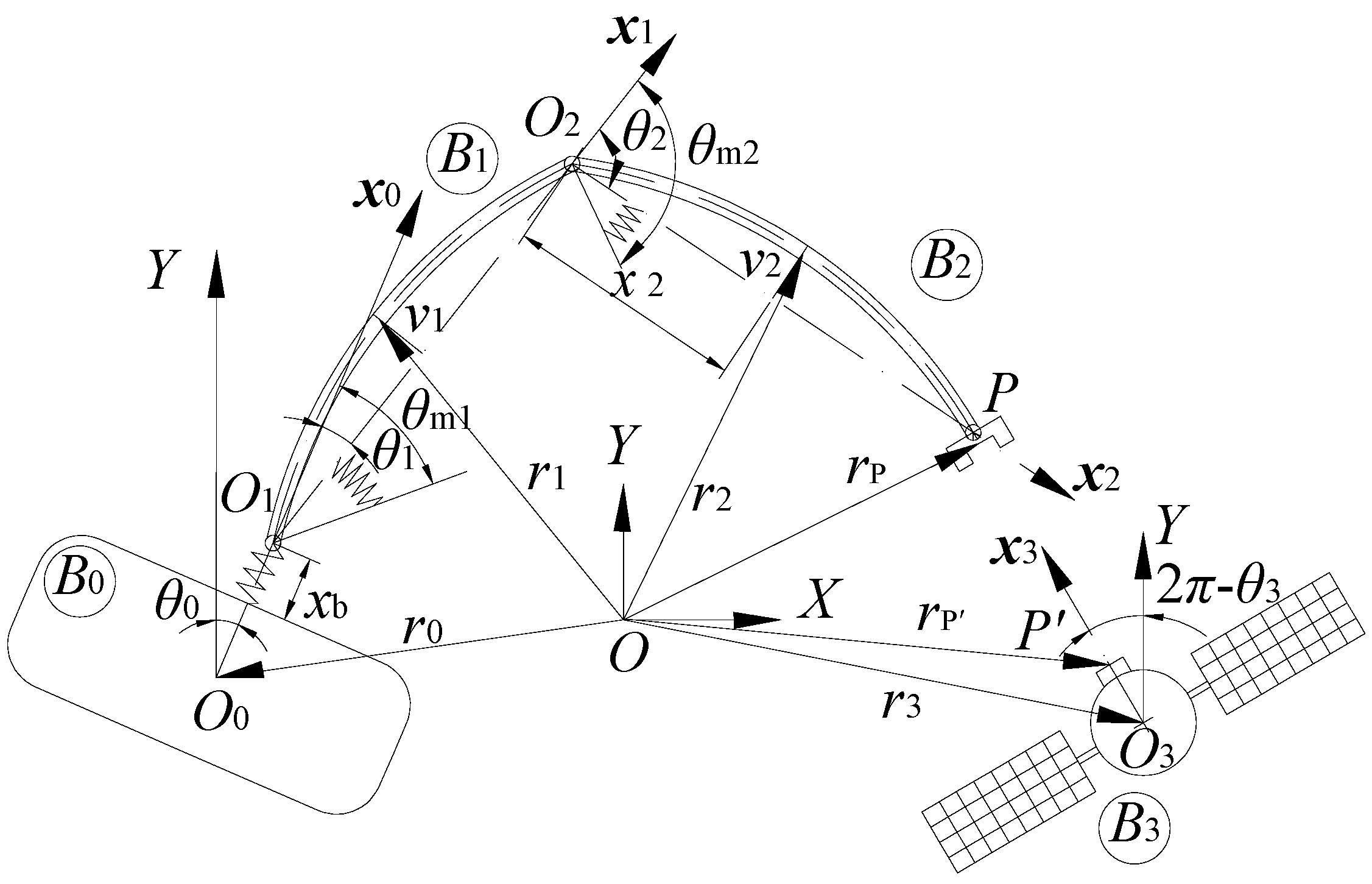
The structure of the flexible-base flexible-link and flexible-joint space robot and the satellite are shown in Figure 1. The space robot comprises a base $B_0$, a flexible link $B_1$ near the base, and a flexible link $B_2$ away from the base. The center of mass of the base is $O_0$, the center of the hinge connecting the base and link $B_1$ is $O_1$, the center of the hinge connecting link $B_1$ and $B_2$ is $O_2$, and the center of mass of the captured satellite is $O_3$. $XOY$ is the inertial coordinate system, and $x_i{O}_i{y}_i$$\left(i=0,1,2,3\right)$ is the local coordinate system of $B_i$. ${\theta }_0$ is the attitude angle of the base, and ${\theta }_j$$\left(j=1,2\right)$ is the rotation angle of link $B_j$. ${\theta }_{m1}$ and ${\theta }_{m2}$ are the rotor angles of the motor, and ${\theta }_3$ is the attitude angle of the satellite. P and P’ are the capture points of the space robot end effector and satellite, respectively. $r_0$, $r_P$, $r_{P^{\prime }}$ and $r_3$ represent the position vectors of the mass center of the base, the capture point of the space robot end effector, the captured point of the satellite and the mass center of the satellite in the inertial coordinate system, respectively. $r_j$ is the position vector of any point on link $B_j$ in the inertial coordinate system. Let $x_j$ be any distance in the symmetry axis direction of the link $B_j$, and let $v_j$$\left(j=1,2\right)$ be the elastic deformation of link $B_j$ at time t.

According to the hypothesis of Spong [26], the flexible base and joint are assumed to be a massless linear telescopic spring and linear torsion spring, respectively. The flexible links are equivalent to the Euler Bernoulli simply supported beam. The elastic coefficients of the base, joints and bending rigidity of the links are fixed, which are expressed as $k_{\mathrm{b}}$, $k_{\mathrm{m}\mathrm{j}}$ and $E{I}_j$$(j=1,2)$, respectively. The deformation of link $B_j$ is $v_j\left(x_j,\mathrm{T}\right)={\displaystyle \sum _{k=1}^n{\varphi }_{jk}\left(x_j\right){\delta }_{jk}\left(t\right)}$, where ${\varphi }_{jk}$ and ${\delta }_{jk}$ represent the kth-order modal function and coordinates of link $B_j$, respectively, and $n$ is the number of reserved modes ($n=2$ in the paper).

The captured satellite is assumed to be a single rigid body system. According to the geometric position relationship of the system, the position vectors ${\mathit{r}}_0$, ${\mathit{r}}_1$, ${\mathit{r}}_2$, ${\mathit{r}}_{\mathrm{P}}$, ${\mathit{r}}_3$ and ${\mathit{r}}_{{\mathrm{P}}^{\prime }}$ are:

$$\{\begin{array}{l}{\mathit{r}}_0={\left(x_0,y_0\right)}^{\mathrm{T}}\\ {\mathit{r}}_1={\mathit{r}}_0+\left(l_0+x_{\mathrm{b}}\right){\mathit{e}}_0+x_1{\mathit{e}}_1+v_1{\mathit{e}}_1^{\prime }, 0 \le x_1\le l_1\\ {\mathit{r}}_2={\mathit{r}}_0+\left(l_0+x_{\mathrm{b}}\right){\mathit{e}}_0+l_1{\mathit{e}}_1+x_2{\mathit{e}}_2+v_2{\mathit{e}}_2^{\prime }, 0 \le x_2\le l_2\\ {\mathit{r}}_{\mathrm{p}}={\mathit{r}}_0+\left(l_0+x_{\mathrm{b}}\right){\mathit{e}}_0+l_1{\mathit{e}}_1+l_2{\mathit{e}}_2\\ {\mathit{r}}_3={\left(x_3,y_3\right)}^{\mathrm{T}}\\ {\mathit{r}}_{{\mathrm{P}}^{\prime }}={\mathit{r}}_3+l_3{\mathit{e}}_3\end{array}$$

(1)

where $\left(x_0,y_0\right)$ are the base centroid coordinate, $l_0$ is the distance between the rotation centers $O_0$ and $O_1$, $x_{\mathrm{b}}$ is the base flexible deformation, $\left(x_3,y_3\right)$ are the satellite centroid coordinate, $l_3$ is the distance between the rotation centers $O_3$ and $P^{\prime }$, ${\mathit{e}}_0$, ${\mathit{e}}_j$, ${\mathit{e}}_j^{\prime }$ $(j=1,2)$ and ${\mathit{e}}_3$ are base vectors.

Taking the differentiation of Equation (1) with respected to time t leads to:

$$\{\begin{array}{l}{\dot{\mathit{r}}}_0={\left({\dot{x}}_0,{\dot{y}}_0\right)}^{\mathrm{T}}\\ {\dot{\mathit{r}}}_1={\dot{\mathit{r}}}_0+{\dot{x}}_{\mathrm{b}}{\mathit{e}}_0+\left(l_0+x_{\mathrm{b}}\right){\dot{\mathit{e}}}_0+x_1{\dot{\mathit{e}}}_1+{\dot{v}}_1{\mathit{e}}_1^{\prime }+v_1{\dot{\mathit{e}}}_1^{\prime }\\ {\dot{\mathit{r}}}_2={\dot{\mathit{r}}}_0+{\dot{x}}_{\mathrm{b}}{\mathit{e}}_0+\left(l_0+x_{\mathrm{b}}\right){\dot{\mathit{e}}}_0+l_1{\dot{\mathit{e}}}_1+x_2{\dot{\mathit{e}}}_2+{\dot{v}}_2{\mathit{e}}_2^{\prime }+v_2{\dot{\mathit{e}}}_2^{\prime }\\ {\dot{\mathit{r}}}_{\mathrm{p}}={\dot{\mathit{r}}}_0+{\dot{x}}_{\mathrm{b}}{\mathit{e}}_0+\left(l_0+x_{\mathrm{b}}\right){\dot{\mathit{e}}}_0+l_1{\dot{\mathit{e}}}_1+l_2{\dot{\mathit{e}}}_2\\ {\dot{\mathit{r}}}_3={\left({\dot{x}}_3,{\dot{y}}_3\right)}^{\mathrm{T}}\\ {\dot{\mathit{r}}}_{{\mathrm{P}}^{\prime }}={\dot{\mathit{r}}}_3+l_3{\dot{\mathit{e}}}_3\end{array}$$

(2)

According to the 4th and 6th equations of Equation (2), the kinematic expressions of the space robot and satellite are as follows:

$$\{\begin{array}{l}{\mathit{V}}_{\mathrm{p}}=\mathit{J}{\dot{\mathit{q}}}_{\mathrm{z}}\\ {\mathit{V}}_{{\mathrm{P}}^{\prime }}={\mathit{J}}_3{\dot{\mathit{q}}}_3\end{array}$$

(3)

where ${\mathit{V}}_{\mathrm{p}}={\left[{\dot{x}}_{\mathrm{p}},{\dot{y}}_{\mathrm{p}},{\omega }_{\mathrm{p}}\right]}^{\mathrm{T}}$, ${\omega }_{\mathrm{p}}={\dot{\theta }}_0+{\dot{\theta }}_1+{\dot{\theta }}_2$, and $\mathit{J}\in {\mathbf{R}}^{3\times 12}$ is the Jacobian matrix of the flexible space robot. ${\dot{\mathit{q}}}_{\mathrm{z}}={\left[{\dot{\mathit{q}}}_{\mathrm{b}},{\dot{x}}_{\mathrm{b}},\dot{\mathit{q}},\dot{\mathit{\delta }},{\dot{\mathit{q}}}_{\mathrm{m}}\right]}^{\mathrm{T}}$, ${\mathit{q}}_{\mathrm{b}}={\left[x_0,y_0\right]}^{\mathrm{T}}$, $\mathit{q}={\left[{\theta }_0,{\theta }_1,{\theta }_2\right]}^{\mathrm{T}}$, $\mathit{\delta }={\left[{\delta }_{11},{\delta }_{12},{\delta }_{21},{\delta }_{22}\right]}^{\mathrm{T}}$

, and ${\mathit{q}}_{\mathrm{m}}={\left[{\theta }_{\mathrm{m}1},{\theta }_{\mathrm{m}2}\right]}^{\mathrm{T}}$. ${\mathit{J}}_3\in {\mathbf{R}}^{3\times 3}$ is the Jacobian matrix of the satellite. ${\mathit{V}}_{{\mathrm{p}}^{\prime }}={\left[{\dot{x}}_{{\mathrm{p}}^{\prime }},{\dot{y}}_{{\mathrm{p}}^{\prime }},{\omega }_{{\mathrm{p}}^{\prime }}\right]}^{\mathrm{T}}$ and ${\omega }_{{\mathrm{p}}^{\prime }}={\dot{\theta }}_3$, ${\dot{\mathit{q}}}_3={\left[{\dot{x}}_3,{\dot{y}}_3,{\dot{\theta }}_3\right]}^{\mathrm{T}}$.

3. System Dynamics Analysis

3.1. Flexible Space Robot and Satellite Dynamics Modeling

The kinetic energy of the flexible space robot is mainly composed of the kinetic energy of the base, links and motor rotors [27], as follows:

$$T=\frac{1}{2}{m}_0{\dot{\mathit{r}}}_0^2+\frac{1}{2}{J}_0{\dot{\theta }}_0^2+{\displaystyle \sum _{j=1}^2\frac{1}{2}{\displaystyle {\int }_0^{l_j}{\rho }_j{\dot{\mathit{r}}}_j^2\mathrm{d}{x}_j}}+{\displaystyle \sum _{j=1}^2\frac{1}{2}{J}_{mj}{\dot{\theta }}_{mj}^2}$$

(4)

where $J_0$ and $J_{mj}$ are the inertia moment of the base and the j-th motor rotor, respectively, and ${\rho }_j$ is the linear density of link $B_j$$(j=1,2)$.

The potential energy of a flexible space robot is mainly composed of a flexible base, flexible joints, and flexible links, as follows:

$$U=\frac{1}{2}{k}_{\mathrm{b}}{x}_{\mathrm{b}}^2+\frac{1}{2}{\displaystyle \sum _{j=1}^2{\displaystyle \sum _{k=1}^2{k}_{\delta jk}{\delta }_{jk}^2}}+{\displaystyle \sum _{j=1}^2\frac{1}{2}{k}_{mj}{\left({\theta }_{mj}-{\theta }_j\right)}^2}$$

(5)

where $k_{\delta jk}=E{I}_j{\displaystyle {\int }_0^{l_j}\left({\ddot{\varphi }}_{jk}^2\left(x_j\right)\right)\mathrm{d}{x}_j},(j,k=1,2)$.

Substituting Equations (4) and (5) into the Lagrange equation yields the space robot dynamic model first equation of Equation (6). Using the Newton–Euler method to calculate the satellite dynamics model the second equation of Equation (6), we have:

$$\{\begin{array}{l}{\mathit{D}}_N{\ddot{\mathit{q}}}_z+{\mathit{H}}_N{\dot{\mathit{q}}}_z+\left[\begin{array}{c}{\mathbf{0}}_{2\times 1}\\ k_{\mathrm{b}}{x}_{\mathrm{b}}\\ 0\\ -{\mathit{K}}_{\mathrm{m}}\mathit{\sigma }\\ {\mathit{K}}_{\mathsf{\delta }}\mathit{\delta }\\ {\mathit{K}}_{\mathrm{m}}\mathit{\sigma }\end{array}\right]=\left[\begin{array}{c}\begin{array}{c}{\mathbf{0}}_{3\times 1}\\ {\tau }_0\\ {\mathbf{0}}_{6\times 1}\end{array}\\ {\mathit{\tau }}_{\mathrm{m}}\end{array}\right]+{\mathit{J}}^{\mathrm{T}}{\mathit{F}}_{\mathrm{P}}\\ {\mathit{D}}_3{\ddot{\mathit{q}}}_3={\mathit{J}}_3^{\mathrm{T}}{\mathit{F}}_{{\mathrm{P}}^{\prime }}\end{array}$$

(6)

where ${\mathit{K}}_{\mathrm{m}}=\mathrm{diag}(k_{\mathrm{m}1},k_{\mathrm{m}2})$, $\mathit{\sigma }={\mathit{q}}_{\mathrm{m}}-{\mathit{q}}_{\mathrm{j}}$, $q_{\mathrm{j}}={\left[{\theta }_1,{\theta }_2\right]}^{\mathrm{T}}$, ${\mathit{q}}_{\mathrm{m}}={\left[q_{\mathrm{m}1},q_{\mathrm{m}2}\right]}^{\mathrm{T}}$, ${\mathit{K}}_{\mathsf{\delta }}=\mathrm{diag}(k_{\mathsf{\delta }11},k_{\mathsf{\delta }12},k_{\mathsf{\delta }21},k_{\mathsf{\delta }22})$, $\mathit{\delta }=[{\delta }_{11},{\delta }_{12},{\delta }_{21},{{\delta }_{22}]}^{\mathrm{T}}$, ${\mathit{D}}_N=\left[\begin{array}{cc}{\mathit{D}}_{10\times 10}& {\mathbf{0}}_{10\times 2}\\ {\mathbf{0}}_{2\times 10}& {\mathit{J}}_{\mathrm{m}}\end{array}\right]$, $\mathit{D}$ is a symmetric positive definite mass matrix, ${\mathit{J}}_{\mathrm{m}}=\mathrm{diag}\left(J_{\mathrm{m}1},J_{\mathrm{m}2}\right)$, ${\mathit{H}}_N=\left[\begin{array}{cc}{\mathit{H}}_{10\times 10}& {\mathbf{0}}_{10\times 2}\\ {\mathbf{0}}_{2\times 10}& {\mathbf{0}}_{2\times 2}\end{array}\right]$, $\mathit{H}$ is the matrix of centrifugal force and Coriolis force, ${\tau }_0$ and ${\mathit{\tau }}_{\mathrm{m}}$ are the control torque of the base and motor rotor, ${\mathit{F}}_{\mathrm{P}}\in {\mathbf{R}}^{3\times 1}$ is the force on the end point $P$ of the robot, ${\mathit{F}}_{{\mathrm{P}}^{\prime }}\in {\mathbf{R}}^{3\times 1}$ is the force on the satellite point $P^{\prime }$, and ${\mathit{D}}_3=\mathrm{diag}\left(m_3,m_3,J_3\right)$.

3.2. Analysis of the Impact Response of the Flexible Space Robot and Satellite

When capturing the satellite, we ignore the effects of other external forces and only consider the impact of the collision. The forces at point $P$ of the space robot end and point $P^{\prime }$ of the satellite are opposite to each other, that is, ${\mathit{F}}_{\mathrm{P}}=-{\mathit{F}}_{{\mathrm{P}}^{\prime }}$. When solving the system dynamics model in a collision process from Equation (6), one obtains:

$${\mathit{D}}_N{\ddot{\mathit{q}}}_z+{\mathit{H}}_N{\dot{\mathit{q}}}_z+\left[\begin{array}{c}{\mathbf{0}}_{2\times 1}\\ k_{\mathrm{b}}{x}_{\mathrm{b}}\\ 0\\ -{\mathit{K}}_{\mathrm{m}}\mathit{\sigma }\\ {\mathit{K}}_{\mathsf{\delta }}\mathit{\delta }\\ {\mathit{K}}_{\mathrm{m}}\mathit{\sigma }\end{array}\right]=\left[\begin{array}{c}\begin{array}{c}{\mathbf{0}}_{3\times 1}\\ {\tau }_0\\ {\mathbf{0}}_{6\times 1}\end{array}\\ {\mathit{\tau }}_{\mathrm{m}}\end{array}\right]-{\mathit{J}}^{\mathrm{T}}{\left({\mathit{J}}_3^{\mathrm{T}}\right)}^{-1}{\mathit{D}}_3{\ddot{\mathit{q}}}_3$$

(7)

During the capture process, the space robot collides with the satellite at time $t_0$, and the capture is completed in a very short time $\Delta t$. Then, the end effector of the space robot tightly connects to the satellite capture point, and the two constitute a system. Because the contact and collision occur instantaneously, the generalized coordinates of the space robot and the satellite do not change significantly in time $\left[t_0,t_0+\Delta t\right]$, but the collision impact causes a sudden change in the generalized velocity and acceleration. According to the analysis above, Equation (7) is integrated in the period $\left[t_0,t_0+\Delta t\right]$ that leads to:

$${\mathit{D}}_N\left[{\dot{\mathit{q}}}_z\left(t_0+\Delta t\right)-{\dot{\mathit{q}}}_z\left(t_0\right)\right]+{\mathit{J}}^{\mathrm{T}}{\left({\mathit{J}}_3^{\mathrm{T}}\right)}^{-1}{\mathit{D}}_3\left[{\dot{\mathit{q}}}_3\left(t_0+\Delta t\right)-{\dot{\mathit{q}}}_3\left(t_{\mathbf{0}}\right)\right]={\mathbf{0}}_{12\times 1}$$

(8)

After capturing, the end effector of the robot will have the same speed as the target capture point. Based on Equation (3), we have:

$${\dot{\mathit{q}}}_3\left(t_0+\Delta t\right)={\mathit{J}}_3^{-1}\mathit{J}{\dot{\mathit{q}}}_z\left(t_0+\Delta t\right)$$

(9)

Substituting Equation (9) into Equation (8) yields:

$${\dot{\mathit{q}}}_z\left(t_0+\Delta t\right)={\left[{\mathit{D}}_N+{\mathit{J}}^{\mathrm{T}}{\left({\mathit{J}}_3^{\mathrm{T}}\right)}^{-1}{\mathit{D}}_3{\mathit{J}}_3^{-1}\mathit{J}\right]}^{-1}\left[{\dot{\mathit{q}}}_z\left(t_0\right)+{\mathit{J}}^{\mathrm{T}}{\left({\mathit{J}}_3^{\mathrm{T}}\right)}^{-1}{\mathit{D}}_3{\dot{\mathit{q}}}_3\left(t_0\right)\right]$$

(10)

The above equations represent the impact effect of the space robot in the process of capturing the satellite. The analysis shows that the generalized speed of the space robot at time $t_0+\Delta t$ can be obtained only by contacting the motion state of the space robot and the satellite before the collision.

3.3. System Dynamics Modeling

After the flexible space robot captures the satellite, it will form a system, and the speed of the space robot end effector and the satellite are equal, that is, ${\mathit{V}}_{\mathrm{p}}={\mathit{V}}_{{\mathrm{P}}^{\prime }}$. Taking the differentiation of that equation, we have:

$${\ddot{\mathit{q}}}_3={\mathit{J}}_3^{-1}\mathit{J}{\ddot{\mathit{q}}}_z+{\mathit{J}}_3^{-1}\left(\dot{\mathit{J}}-{\dot{\mathit{J}}}_3{\mathit{J}}_3^{-1}\mathit{J}\right){\dot{\mathit{q}}}_z$$

(11)

Substituting Equation (11) into the second equation of Equation (6), we have ${\mathit{F}}_{{\mathrm{P}}^{\prime }}$. ${\mathit{F}}_{\mathrm{P}}={\mathit{F}}_{{\mathrm{P}}^{\prime }}$. Substituting ${\mathit{F}}_{\mathrm{P}}$ into first equation of Equation (6), we have:

$${\mathit{D}}_z{\ddot{\mathit{q}}}_z+{\mathit{H}}_z{\dot{\mathit{q}}}_z+\left[\begin{array}{c}{\mathbf{0}}_{2\times 1}\\ k_{\mathrm{b}}{x}_{\mathrm{b}}\\ 0\\ -{\mathit{K}}_{\mathrm{m}}\mathit{\sigma }\\ {\mathit{K}}_{\mathsf{\delta }}\mathit{\delta }\\ {\mathit{K}}_{\mathrm{m}}\mathit{\sigma }\end{array}\right]=\left[\begin{array}{c}\begin{array}{c}{\mathbf{0}}_{3\times 1}\\ {\tau }_0\\ {\mathbf{0}}_{6\times 1}\end{array}\\ {\mathit{\tau }}_{\mathrm{m}}\end{array}\right]$$

(12)

where ${\mathit{D}}_z={\mathit{D}}_N+{\mathit{J}}^{\mathrm{T}}{\left({\mathit{J}}_3^{\mathrm{T}}\right)}^{-1}{\mathit{D}}_3{\mathit{J}}_3^{-1}\mathit{J}$ and ${\mathit{H}}_z={\mathit{H}}_N+{\mathit{J}}^{\mathrm{T}}{\left({\mathit{J}}_3^{\mathrm{T}}\right)}^{-1}{\mathit{D}}_3{\mathit{J}}_3^{-1}\left(\dot{\mathit{J}}-{\dot{\mathit{J}}}_3{\mathit{J}}_3^{-1}\mathit{J}\right)$. For the convenience of later analysis, ${\mathit{D}}_z$ and ${\mathit{H}}_z$ are written in the form of a block matrix, as follows:

$${\mathit{D}}_z=\left[\begin{array}{ccc}{\mathit{D}}_{z11}& {\mathit{D}}_{z12}& {\mathbf{0}}_{2\times 2}\\ {\mathit{D}}_{z21}& {\mathit{D}}_{z22}& {\mathbf{0}}_{8\times 2}\\ {\mathbf{0}}_{2\times 2}& {\mathbf{0}}_{2\times 8}& {\mathit{J}}_{\mathrm{m}}\end{array}\right],{\mathit{H}}_z=\left[\begin{array}{ccc}{\mathbf{0}}_{2\times 2}& {\mathit{H}}_{z12}& {\mathbf{0}}_{2\times 2}\\ {\mathbf{0}}_{8\times 2}& {\mathit{H}}_{z22}& {\mathbf{0}}_{8\times 2}\\ {\mathbf{0}}_{2\times 2}& {\mathbf{0}}_{2\times 8}& {\mathbf{0}}_{2\times 2}\end{array}\right].$$

Based on controller design needs, Equation (12) is rewritten as:

$$\left[\begin{array}{cc}{\mathit{D}}_{z11}& {\mathit{D}}_{z12}\\ {\mathit{D}}_{z21}& {\mathit{D}}_{z22}\end{array}\right]\left[\begin{array}{c}{\ddot{\mathit{q}}}_{\mathrm{b}}\\ {\ddot{x}}_{\mathrm{b}}\\ \ddot{\mathit{q}}\\ \ddot{\mathit{\delta }}\end{array}\right]+\left[\begin{array}{cc}{\mathbf{0}}_{2\times 2}& {\mathit{H}}_{\mathrm{z}12}\\ {\mathbf{0}}_{8\times 2}& {\mathit{H}}_{\mathrm{z}22}\end{array}\right]\left[\begin{array}{c}{\dot{\mathit{q}}}_{\mathrm{b}}\\ {\dot{x}}_{\mathrm{b}}\\ \dot{\mathit{q}}\\ \dot{\mathit{\delta }}\end{array}\right]+\left[\begin{array}{c}{\mathbf{0}}_{2\times 1}\\ k_{\mathrm{b}}{x}_{\mathrm{b}}\\ 0\\ -\mathit{\tau }\\ {\mathit{K}}_{\mathsf{\delta }}\mathit{\delta }\end{array}\right]=\left[\begin{array}{c}{\mathbf{0}}_{3\times 1}\\ {\tau }_0\\ {\mathbf{0}}_{6\times 1}\end{array}\right]$$

(13)

$${\mathit{J}}_{\mathrm{m}}{\ddot{\mathit{q}}}_{\mathrm{m}}+{\mathit{K}}_{\mathrm{m}} \mathit{\sigma }={\mathit{\tau }}_{\mathrm{m}}$$

(14)

$$\mathit{\tau }={\mathit{K}}_{\mathrm{m}}\mathit{\sigma }$$

(15)

After calculating ${\ddot{\mathit{q}}}_{\mathrm{b}}$ from the first formula of Equation (13) and substituting it into the second formula, we have:

$${\mathit{D}}_{\mathrm{M}}\left[\begin{array}{c}{\ddot{x}}_{\mathrm{b}}\\ \ddot{\mathit{q}}\\ \ddot{\mathit{\delta }}\end{array}\right]+{\mathit{H}}_{\mathrm{M}}\left[\begin{array}{c}{\dot{x}}_{\mathrm{b}}\\ \dot{\mathit{q}}\\ \dot{\mathit{\delta }}\end{array}\right]+\left[\begin{array}{c}{k}_{\mathrm{b}}{x}_{\mathrm{b}}\\ {\mathbf{0}}_{3\times 1}\\ {\mathit{K}}_{\mathsf{\delta }}\mathit{\delta }\end{array}\right]=\left[\begin{array}{c}0\\ {\tau }_0\\ \mathit{\tau }\\ {\mathbf{0}}_{4\times 1}\end{array}\right]$$

(16)

where ${\mathit{D}}_{\mathrm{M}}={\mathit{D}}_{\mathrm{z}22}-{\mathit{D}}_{\mathrm{z}21}{({\mathit{D}}_{\mathrm{z}11})}^{-1}{\mathit{D}}_{\mathrm{z}12}$, ${\mathit{H}}_{\mathrm{M}}={\mathit{H}}_{\mathrm{z}22}-{\mathit{D}}_{\mathrm{z}21}{({\mathit{D}}_{\mathrm{z}11})}^{-1}{\mathit{H}}_{\mathrm{z}12}$, and ${\mathit{D}}_{\mathrm{M}}$ and ${\mathit{H}}_{\mathrm{M}}$ are written in the form of a block matrix, as follows:

$${\mathit{D}}_{\mathrm{M}}=\left[\begin{array}{cc}{\mathit{D}}_{\mathrm{M}11}& {\mathit{D}}_{\mathrm{M}12}\\ {\mathit{D}}_{\mathrm{M}21}& {\mathit{D}}_{\mathrm{M}22}\end{array}\right],{\mathit{H}}_{\mathrm{M}}=\left[\begin{array}{cc}{\mathit{H}}_{\mathrm{M}11}& {\mathit{H}}_{\mathrm{M}12}\\ {\mathit{H}}_{\mathrm{M}21}& {\mathit{H}}_{\mathrm{M}22}\end{array}\right]$$

4. Singular Perturbation Decomposition of the System

The flexible space robot after capturing the satellite is a complex nonlinear rigid-flexible coupling system. Using the singular perturbation method, the system is decomposed into a slow subsystem including a base, joint motion, and link vibration. The fast subsystem involves base vibration and joint vibration. The control torque of the joint motor is designed as follows:

$${\mathit{\tau }}_m=\left(\mathit{I}+{\mathit{K}}_c\right){\mathit{\tau }}_n-{\mathit{K}}_c\mathit{\tau }$$

(17)

where ${\mathit{K}}_c$ is a joint flexibility compensator and ${\mathit{\tau }}_n$ is composed of a slow sub-controller ${\mathit{\tau }}_{ns}$ and a fast sub-controller ${\mathit{\tau }}_{nf}$.

Let $\mathit{N}=\left[\begin{array}{cc}{\mathit{N}}_{11}& {\mathit{N}}_{12}\\ {\mathit{N}}_{21}& {\mathit{N}}_{22}\end{array}\right]={\left[\begin{array}{cc}{\mathit{D}}_{M11}& {\mathit{D}}_{M12}\\ {\mathit{D}}_{M21}& {\mathit{D}}_{M22}\end{array}\right]}^{-1}$. We define ${\mathrm{T}}_f=\mathrm{T}/\sqrt{\mu }$ as the fast-changing timescale, and $\mu =1/\min \left(k_{\mathrm{b}},k_{\mathrm{m}1},k_{\mathrm{m}2}\right)$ as the singular perturbation factor. The state variables of the system under a fast timescale are ${\mathit{q}}_f=[q_{f1},q_{f2},{{\mathit{q}}_{f3}^{\mathrm{T}},{\mathit{q}}_{f4}^{\mathrm{T}}]}^{\mathrm{T}}$, where $q_{f1}=x_{bf}-{\overline{x}}_{bf}$, $q_{f2}=\sqrt{\mu }{\overline{x}}_{bf}$, ${\mathit{q}}_{f3}={\mathit{\sigma }}_f-{\overline{\mathit{\sigma }}}_f$, and ${\mathit{q}}_{f4}=\sqrt{\mu }{\dot{\mathit{\sigma }}}_f$. $\overline{\ast }$ is a new expression of $\ast$ when $\mu$ tends to zero, and ${\ast }_f$ is a new variable of $\ast$ under a fast timescale. From the above variables and Equations (14)–(17), the slow subsystem of the system is obtained as follows:

$$\left[\begin{array}{cc}{\mathit{Q}}_{11}& {\mathit{Q}}_{12}\\ {\mathit{Q}}_{21}& {\mathit{Q}}_{22}\end{array}\right]\left[\begin{array}{c}\ddot{\mathit{q}}\\ \ddot{\mathit{\delta }}\end{array}\right]+\left[\begin{array}{cc}{\mathit{R}}_{11}& {\mathit{R}}_{12}\\ {\mathit{R}}_{21}& {\mathit{R}}_{22}\end{array}\right]\left[\begin{array}{c}\dot{\mathit{q}}\\ \dot{\mathit{\delta }}\end{array}\right]+\left[\begin{array}{c}\mathbf{0}\\ {\mathbf{0}}_{2\times 1}\\ {\mathit{K}}_{\mathsf{\delta }}\mathit{\delta }\end{array}\right]=\left[\begin{array}{c}{\tau }_0\\ {\mathit{\tau }}_{\mathrm{ns}}\\ {\mathbf{0}}_{4\times 1}\end{array}\right]$$

(18)

where ${\mathit{Q}}_{11}\in {\mathit{R}}^{3\times 3}$, ${\mathit{Q}}_{12}\in {\mathit{R}}^{3\times 4}$, ${\mathit{Q}}_{21}\in {\mathit{R}}^{4\times 3}$, ${\mathit{Q}}_{22}\in {\mathit{R}}^{4\times 4}$, ${\mathit{R}}_{11}\in {\mathit{R}}^{3\times 3}$, ${\mathit{R}}_{12}\in {\mathit{R}}^{3\times 4}$, ${\mathit{R}}_{21}\in {\mathit{R}}^{4\times 3}$, ${\mathit{R}}_{22}\in {\mathit{R}}^{4\times 4}$, $\left[\begin{array}{cc}{\mathit{Q}}_{11}& {\mathit{Q}}_{12}\\ {\mathit{Q}}_{21}& {\mathit{Q}}_{22}\end{array}\right]={\overline{\mathit{D}}}_{M22}+\left[\begin{array}{ccc}0& {\mathbf{0}}_{1\times 2}& {\mathbf{0}}_{1\times 4}\\ {\mathbf{0}}_{2\times 1}& {\left(\mathit{I}+{\mathit{K}}_c\right)}^{-1}{\mathit{J}}_m& {\mathbf{0}}_{2\times 4}\\ {\mathbf{0}}_{4\times 1}& {\mathbf{0}}_{4\times 2}& {\mathbf{0}}_{4\times 4}\end{array}\right]$, and $\left[\begin{array}{cc}{\mathit{R}}_{11}& {\mathit{R}}_{12}\\ {\mathit{R}}_{21}& {\mathit{R}}_{22}\end{array}\right]={\overline{\mathit{H}}}_{M22}$.

The fast subsystem of the system is as follows:

$$\mathrm{d}{\mathit{q}}_{\mathrm{f}}/\mathrm{d}{\mathit{t}}_{\mathrm{f}}={\mathit{A}}_{\mathrm{f}}{\mathit{q}}_{\mathrm{f}}+{\mathit{B}}_{\mathrm{f}}{\mathit{\tau }}_{\mathrm{nf}}$$

(19)

where ${\mathit{B}}_{\mathrm{f}}={\left[{\mathbf{0}}_{4\times 2}^{\mathrm{T}},{\left[{\mathit{J}}_{\mathrm{m}}^{-1}\left(\mathit{I}+{\mathit{K}}_{\mathrm{c}}\right)\right]}^{\mathrm{T}}\right]}^{\mathrm{T}}$ and ${\mathit{A}}_{\mathrm{f}}=\left[\begin{array}{cccc}0& 1& {\mathbf{0}}_{1\times 2}& {\mathbf{0}}_{1\times 2}\\ -{\overline{\mathit{N}}}_{11}{k}_{\mathrm{b}\mathrm{f}}& 0& {\mathit{N}}_{12}^{\ast }{\mathit{K}}_{\mathrm{mf}}& {\mathbf{0}}_{1\times 2}\\ {\mathbf{0}}_{2\times 1}& {\mathbf{0}}_{2\times 1}& {\mathbf{0}}_{2\times 2}& {\mathit{I}}_{2\times 2}\\ {\mathbf{0}}_{2\times 1}& {\mathbf{0}}_{2\times 1}& -{\mathit{J}}_{\mathrm{m}}^{-1}\left(\mathit{I}+{\mathit{K}}_{\mathrm{c}}\right){\mathit{K}}_{\mathrm{mf}}& {\mathbf{0}}_{2\times 2}\end{array}\right]$.

By introducing the second equation of Equation (18) into the first equation, the rigid model of the slow subsystem is obtained [28,29] as follows:

$$\mathit{M}(\mathit{q},\mathit{\delta })\ddot{\mathit{q}}+\mathit{C}(\mathit{q},\mathit{\delta },\dot{\mathit{q}},\dot{\mathit{\delta }})\dot{\mathit{q}}+\xi (\mathit{q},\mathit{\delta },\dot{\mathit{q}},\dot{\mathit{\delta }})=\mathit{u}$$

(20)

where $\mathit{M}={\mathit{Q}}_{11}-{\mathit{Q}}_{12}{\mathit{Q}}_{22}^{-1}{\mathit{Q}}_{21}$, $\mathit{C}={\mathit{R}}_{11}-{\mathit{Q}}_{12}{\mathit{Q}}_{22}^{-1}{\mathit{R}}_{21}$, $\xi =\left({\mathit{R}}_{12}-{\mathit{Q}}_{12}{\mathit{Q}}_{22}^{-1}{\mathit{R}}_{22}\right)\dot{\mathit{\delta }}-{\mathit{Q}}_{12}{\mathit{Q}}_{22}^{-1}{\mathit{K}}_{\delta }\mathit{\delta }$, $\mathit{u}={\left[{\tau }_0,{\mathit{\tau }}_{ns}^{\mathrm{T}}\right]}^{\mathrm{T}}$, and $\mathit{C}\left(\mathit{x},\mathit{y}\right)$ meet $\mathit{C}\left(\mathit{x},\mathit{y}\right)\mathit{z}=\mathit{C}\left(\mathit{x},\mathit{z}\right)\mathit{y}, \forall \mathit{y},\mathit{z}\in {\mathbf{R}}^{3\times 1}$.

5. Controller Design

5.1. Controller Design of the Slow Subsystem

5.1.1. Repetitive Learning Sliding Mode Control

For the slow subsystem rigid model Equation (20), define the continuous reference signal with period T as ${\mathit{q}}_{\mathrm{d}}={\left[{\theta }_{\mathrm{d}0},{\theta }_{\mathrm{d}1},{\theta }_{\mathrm{d}2}\right]}^{\mathrm{T}}$ and substitute it into Equation (20) to get:

$$\{\begin{array}{l}{\mathit{u}}_{\mathrm{d}}=\mathit{M}\left({\mathit{q}}_{\mathrm{d}}\right){\ddot{\mathit{q}}}_{\mathrm{d}}+\mathit{C}\left({\mathit{q}}_{\mathrm{d}},{\dot{\mathit{q}}}_{\mathrm{d}}\right){\dot{\mathit{q}}}_{\mathrm{d}}+\mathit{\xi }\left({\mathit{q}}_{\mathrm{d}},{\dot{\mathit{q}}}_{\mathrm{d}}\right)\\ {\mathit{u}}_{\mathrm{d}}\left(t\right)={\mathit{u}}_{\mathrm{d}}\left(t+T\right)\end{array}$$

(21)

Expand the periodic function ${\mathit{u}}_{\mathrm{d}}$ with an infinite-dimensional Fourier series as:

$${\mathit{u}}_{\mathrm{d}}={\overline{\mathit{\partial }}}_0+{\displaystyle \sum _{k=1}^{\infty }\left[{\overline{\mathit{\partial }}}_k\cos \left(k\omega t\right)+{\overline{\mathit{\beta }}}_k\sin \left(k\omega t\right)\right]}$$

(22)

where $\omega =2\pi /T$ is the fundamental frequency, and ${\overline{\mathit{\partial }}}_0$, ${\overline{\mathit{\partial }}}_k$ and ${\overline{\mathit{\beta }}}_k$ are the unknown constant vector.

After defining the trajectory tracking error $\mathit{e}={\mathit{q}}_{\mathrm{d}}-\mathit{q}$, the exponential approach law sliding mode vector $\mathit{s}\in {\mathbf{R}}^{3\times 1}$ is:

$$\mathit{s}=\dot{\mathit{e}}+a\mathit{e}+b{\mathit{e}}^{(q/p)}$$

(23)

where $a$, $b$, $p$ and $q$ are positive constants.

Equation (23) takes the derivative of time t to get:

$$\dot{\mathit{s}}=\ddot{\mathit{e}}+a\dot{\mathit{e}}+b\frac{q}{p}{\mathit{e}}^{\left(\frac{q}{p}-1\right)}$$

(24)

Multiply both sides of Equation (24) to the left by $\mathit{M}$ at the same time, and we obtain the error equation of the open loop system as follows:

$$\mathit{M}\dot{\mathit{s}}=-\mathit{C}\mathit{s}+\mathit{Y}+a\mathit{M}\dot{\mathit{e}}+b\frac{q}{p}\mathit{M}{\mathit{e}}^{\left(\frac{q}{p}-1\right)}+{\mathit{u}}_{\mathrm{d}}-\mathit{u}$$

(25)

$$\mathit{Y}=\mathit{M}{\ddot{\mathit{q}}}_{\mathrm{d}}+\mathit{C}\left({\dot{\mathit{q}}}_{\mathrm{d}}+a\mathit{e}+b{\mathit{e}}^{(q/p)}\right)+\xi -{\mathit{u}}_{\mathrm{d}}$$

(26)

From Equation (26), we have:

$$\mathit{Y}\le {\kappa }_1\Vert \mathit{h}\Vert +{\kappa }_2{\Vert \mathit{h}\Vert }^2$$

(27)

where ${\kappa }_1$ and ${\kappa }_2$ are positive constants, $\mathit{h}={\left[{\left(a\mathit{e}+b{\mathit{e}}^{(q/p)}\right)}^{\mathrm{T}},{\mathit{s}}^{\mathrm{T}}\right]}^{\mathrm{T}}$.

Design the repetitive learning sliding mode control algorithm as follows:

$$\mathit{u}={\mathit{Q}}_0{\mathit{z}}_0+{\displaystyle \sum _{k=1}^N{\mathit{Q}}_k{\dot{\mathit{z}}}_k }+{\mathit{{\rm K}}}_M\left(a\dot{\mathit{e}}+b\frac{q}{p}{\mathit{e}}^{\left(\frac{q}{p}-1\right)}\right)+\mathit{\eta }$$

(28)

$${\ddot{\mathit{z}}}_k={\mathit{Q}}_k\mathit{s}-k^2{\omega }^2{\mathit{z}}_k,k=1,\cdots N$$

(29)

$${\dot{\mathit{z}}}_0={\mathit{Q}}_0\mathit{s}$$

(30)

where $\mathit{S}\mathit{g}\mathit{n}\left(\mathit{s}\right)={\left[\mathrm{sgn}\left(s_1^{}\right),\mathrm{sgn}\left(s_2^{}\right),\mathrm{sgn}\left(s_3^{}\right)\right]}_{}^T$, $N$ is the number of harmonic oscillators, and $\mathit{\eta }=\left({\mathit{{\rm K}}}_1\Vert a\dot{\mathit{e}}+b\frac{q}{p}{\mathit{e}}^{\left(\frac{q}{p}-1\right)}\Vert +{\mathit{{\rm K}}}_2\Vert \mathit{h}\Vert +{\mathit{{\rm K}}}_3{\Vert \mathit{h}\Vert }^2+{\mathit{{\rm K}}}_d\right)\mathit{S}\mathit{g}\mathit{n}\left(\mathit{s}\right)$.

Define variables as follows:

$$\{\begin{array}{l}{\tilde{\mathit{z}}}_k={\mathit{z}}_k-{\mathit{z}}_k^{\ast }, k=0,1,\cdots N \\ {\mathit{z}}_0^{\ast }={\mathit{Q}}_0^{-1}{\overline{\mathit{\partial }}}_0\\ {\mathit{z}}_k^{\ast }={\left(k\omega \right)}^{-1}{\mathit{Q}}_k^{-1}\left[{\overline{\mathit{\beta }}}_k\cos \left(k\omega t\right)-{\overline{\mathit{\partial }}}_k\sin \left(k\omega t\right)\right]\end{array}$$

(31)

Substituting Equations (28)–(31) into Equation (25), we have:

$$\begin{gathered} \mathit{M}\dot{\mathit{s}}=-\mathit{C}\mathit{s}-{\mathit{Q}}_0{\tilde{\mathit{z}}}_0-{\displaystyle \sum _{k=1}^N{\mathit{Q}}_k{\dot{\tilde{\mathit{z}}}}_k +a\mathit{M}\dot{\mathit{e}}+b\frac{q}{p}\mathit{M}{\mathit{e}}^{\left(\frac{q}{p}-1\right)} +}\mathit{Y}-\mathit{\eta }- \\ {\mathit{{\rm K}}}_M\left(a\dot{\mathit{e}}+b\frac{q}{p}{\mathit{e}}^{\left(\frac{q}{p}-1\right)}\right)+{\displaystyle \sum _{k=N+1}^{\infty }\left[{\overline{\mathit{\partial }}}_k\cos \left(k\omega t\right)+{\overline{\mathit{\beta }}}_k\sin \left(k\omega t\right)\right]} \end{gathered}$$

(32)

$$\{\begin{array}{l}{\ddot{\tilde{\mathit{z}}}}_k={\mathit{Q}}_k\mathit{s}-k^2{\omega }^2{\tilde{\mathit{z}}}_k\\ {\dot{\tilde{\mathit{z}}}}_0={\mathit{Q}}_0\mathit{s}\\ {\mathit{k}}_0={\displaystyle \sum _{k=N+1}^{\infty }\left[{\overline{\mathit{\partial }}}_k\cos \left(k\omega t\right)+{\overline{\mathit{\beta }}}_k\sin \left(k\omega t\right)\right]}\end{array}$$

(33)

Theorem 1.

For the rigid model equation (Equation (20)) of the slow subsystem, if the controller gain satisfies the condition shown in the following equation (Equation (34)), the proposed repetitive learning sliding mode control can guarantee $\underset{t\to \infty }{\lim }\mathit{e}=\mathbf{0}$and$\underset{t\to \infty }{\lim }\dot{\mathit{e}}=\mathbf{0}$.

$$\Vert \mathit{M}-{\mathit{{\rm K}}}_M\Vert \le {\mathit{{\rm K}}}_1, {\kappa }_1\le {\mathit{{\rm K}}}_2, {\kappa }_2\le {\mathit{{\rm K}}}_3, \Vert \mathit{d}\Vert <{\lambda }_m\left({\mathit{{\rm K}}}_{\mathrm{d}}\right)$$

(34)

where $\mathit{d}={\displaystyle \sum _{k=N+1}^{\infty }\left[{\overline{\mathit{\partial }}}_k\cos \left(k\omega t\right)+{\overline{\mathit{\beta }}}_k\sin \left(k\omega t\right)\right]}$.

Proof.

Selecting Lyapunov function as:

$$V=\frac{1}{2}{\mathit{s}}^T\mathit{M}\mathit{s}+\frac{1}{2}{\displaystyle \sum _{k=1}^N{\dot{\tilde{\mathit{z}}}}_k^T{\dot{\tilde{\mathit{z}}}}_k}+\frac{1}{2}{\omega }^2{\displaystyle \sum _{k=1}^N{k}^2{\tilde{\mathit{z}}}_k^T{\tilde{\mathit{z}}}_k}+\frac{1}{2}{\tilde{\mathit{z}}}_0^T{\tilde{\mathit{z}}}_0$$

(35)

Taking the differentiation of Equation (35) with respected to time t, and substituting into Equations (27), (32) and (33) and $\mathit{\eta }$, we have:

$$\begin{gathered} \begin{array}{l}\dot{V}=s^T\left(a\mathit{M}\dot{\mathit{e}}+b\frac{q}{p}\mathit{M}{\mathit{e}}^{\left(\frac{q}{p}-1\right)}\right)-{\mathit{s}}^T{\mathit{{\rm K}}}_M\left(a\dot{\mathit{e}}+b\frac{q}{p}{\mathit{e}}^{\left(\frac{q}{p}-1\right)}\right)+\\ {\mathit{s}}^T{\displaystyle \sum _{k=N+1}^{\infty }\left[{\overline{\mathit{\partial }}}_k\cos \left(k\omega t\right)+{\overline{\mathit{\beta }}}_k\sin \left(k\omega t\right)\right]}+{\mathit{s}}^T\mathit{Y}-{\mathit{s}}^T\mathit{\eta }\\ \le -\Vert \mathit{s}\Vert \left({\mathit{{\rm K}}}_1-\Vert \mathit{M}-{\mathit{{\rm K}}}_M\Vert \right)\Vert a\dot{\mathit{e}}+b\frac{q}{p}{\mathit{e}}^{\left(\frac{q}{p}-1\right)}\Vert -\Vert \mathit{s}\Vert \left({\mathit{{\rm K}}}_2-{\kappa }_1\right)\Vert \mathit{h}\Vert -\end{array} \\ \Vert \mathit{s}\Vert \left({\mathit{{\rm K}}}_3-{\kappa }_2\right){\Vert \mathit{h}\Vert }^2-\left({\lambda }_m\left({\mathit{{\rm K}}}_d\right)-\Vert \mathit{d}\Vert \right)\Vert \mathit{s}\Vert \end{gathered}$$

(36)

when the controller parameters satisfy the stability condition Equation (34), $\dot{V}<0$ is obtained from Equation (36), so the system is stable. □

5.1.2. Repetitive Learning Sliding Mode Control based on the Concept of Virtual Force

The rigid model of the slow subsystem has the effect of link elasticity. This section uses the principle of virtual control force to improve the originally desired trajectory and generate a hybrid trajectory. The improved repetitive learning sliding mode control is designed to realize the dual functions of trajectory tracking and link elastic vibration suppression. The virtual force $\mathit{F}\in {\mathbf{R}}^{3\times 1}$ is defined by the second-order instruction generator ${\ddot{\mathit{e}}}_{\mathrm{h}}+\mathit{a}{\dot{\mathit{e}}}_{\mathrm{h}}+\mathit{b}{\mathit{e}}_{\mathrm{h}}=\mathit{F}$, where ${\mathit{e}}_{\mathrm{h}}={\mathit{q}}_{\mathrm{d}}-{\mathit{q}}_{\mathrm{h}}$ and ${\mathit{q}}_{\mathrm{h}}$ is the hybrid trajectory.

Define the hybrid error ${\mathit{e}}_{\mathrm{r}}={\mathit{q}}_{\mathrm{h}}-\mathit{q}$ and the hybrid exponential sliding mode variable as ${\mathit{s}}_{\mathrm{r}}={\dot{\mathit{e}}}_{\mathrm{r}}+a{\mathit{e}}_{\mathrm{r}}+b{\mathit{e}}_{\mathrm{r}}^{(q/p)}$, modify ${\mathit{q}}_{\mathrm{d}}$ in Equations (28)–(30) to ${\mathit{q}}_{\mathrm{h}}$, and design a repetitive learning sliding mode control based on the concept of virtual force as:

$${\mathit{u}}_{\mathrm{r}}={\mathit{Q}}_0{\mathit{z}}_{0\mathrm{r}}+{\displaystyle \sum _{k=1}^N{\mathit{Q}}_k{\dot{\mathit{z}}}_{k\mathrm{r}} }+{\mathit{{\rm K}}}_M\left(a{\dot{\mathit{e}}}_{\mathrm{r}}+b\frac{q}{p}{\mathit{e}}_{\mathrm{r}}^{\left(\frac{q}{p}-1\right)}\right)+{\mathit{\eta }}_{\mathrm{r}}$$

(37)

$${\ddot{\mathit{z}}}_k={\mathit{Q}}_k{\mathit{s}}_{\mathrm{r}}-k^2{\omega }^2{\mathit{z}}_{k\mathrm{r}},k=1,\cdots N$$

(38)

$${\dot{\mathit{z}}}_{0\mathrm{r}}={\mathit{Q}}_0{\mathit{s}}_{\mathrm{r}}$$

(39)

where ${\mathit{\eta }}_{\mathrm{r}}=\left({\mathit{{\rm K}}}_1\Vert a{\dot{\mathit{e}}}_{\mathrm{r}}+b\frac{q}{p}{\mathit{e}}_{\mathrm{r}}^{\left(\frac{q}{p}-1\right)}\Vert +{\mathit{{\rm K}}}_2\Vert {\mathit{h}}_{\mathrm{r}}\Vert +{\mathit{{\rm K}}}_3{\Vert {\mathit{h}}_{\mathrm{r}}\Vert }^2+{\mathit{{\rm K}}}_d\right)\mathit{S}\mathit{g}\mathit{n}\left({\mathit{s}}_{\mathrm{r}}\right)$.

Let ${\mathit{W}}_{\mathrm{s}}={\left[{\mathit{\delta }}^{\mathrm{T}},{\mathit{e}}^{\mathrm{T}},{\dot{\mathit{\delta }}}^{\mathrm{T}},{\dot{\mathit{e}}}^{\mathrm{T}}\right]}^{\mathrm{T}}$. After substituting the controller equations (Equations (37)–(39)) into Equation (20), and then taking the resulting equation into the derivative of ${\mathit{W}}_{\mathrm{s}}$, we have:

$${\dot{\mathit{W}}}_{\mathrm{s}}={\mathit{A}}_{\mathrm{s}}{\mathit{W}}_{\mathrm{s}}+{\mathit{B}}_{\mathrm{s}}\mathit{F}+{\mathit{L}}_{\mathrm{s}}$$

(40)

where ${\mathit{A}}_s=\left[\begin{array}{cccc}{\mathbf{0}}_{4\times 4}& {\mathbf{0}}_{4\times 3}& {\mathit{I}}_{4\times 4}& {\mathbf{0}}_{4\times 3}\\ {\mathbf{0}}_{3\times 4}& {\mathbf{0}}_{3\times 3}& {\mathbf{0}}_{3\times 4}& {\mathit{I}}_{3\times 3}\\ -{\mathit{Q}}_{22}^{-1}{\mathit{{\rm K}}}_{\mathsf{\delta }}& -{\mathit{Q}}_{22}^{-1}{\mathit{Q}}_{21}\mathit{b}& -{\mathit{Q}}_{22}^{-1}{\mathit{R}}_{22}& -{\mathit{Q}}_{22}^{-1}{\mathit{Q}}_{21}\mathit{a}\\ {\mathbf{0}}_{3\times 4}& -\mathit{b}& {\mathbf{0}}_{3\times 4}& -\mathit{a}\end{array}\right]$, ${\mathit{B}}_s=\left[\begin{array}{c}{\mathbf{0}}_{4\times 3}\\ {\mathbf{0}}_{3\times 3}\\ {\mathit{Q}}_{22}{\mathit{Q}}_{21}\\ {\mathit{I}}_{3\times 3}\end{array}\right]$, and ${\mathit{L}}_s=\left[\begin{array}{c}{\mathbf{0}}_{4\times 1}\\ {\mathbf{0}}_{3\times 1}\\ {\mathit{Q}}_{22}^{-1}{\mathit{Q}}_{21}\left(\mathit{G}-{\ddot{\mathit{q}}}_{\mathrm{d}}\right)-{\mathit{Q}}_{22}^{-1}{\mathit{R}}_{21}\dot{\mathit{q}}\\ \mathit{G}\end{array}\right]$.

Select virtual force $\mathit{F}$ as:

$$\mathit{F}=-{\mathit{Q}}_{\mathrm{s}}^{-1}{\mathit{B}}_{\mathrm{s}}^{\mathrm{T}}{\mathit{P}}_{\mathrm{s}} {\mathit{W}}_{\mathrm{s}}$$

(41)

where ${\mathit{P}}_{\mathrm{s}}$ is the solution of the Riccati equation.

When $\mathit{F}$ takes the value shown in Equation (41), Equation (40) is stable. Stability proof refers to Lee et al. [30].

5.2. Controller Design of the Fast Subsystem

The above two sections mainly design the controller for the slow subsystem. In this section, based on the fast subsystem, Equation (19), the control scheme to suppress the flexible vibration of the base and joint is designed. The performance index function is constructed as follows:

$$J_{\mathrm{q}\mathrm{f}}=\frac{1}{2}{\displaystyle {\int }_0^{\infty }\left({\mathit{q}}_{\mathrm{f}}^{\mathrm{T}}{\mathit{Q}}_{\mathrm{f}}{\mathit{q}}_{\mathrm{f}}+{\mathit{\tau }}_{\mathrm{n}\mathrm{f}}^{\mathrm{T}}{\mathit{R}}_{\mathrm{f}}{\mathit{\tau }}_{\mathrm{n}\mathrm{f}}\right)}\mathrm{d}{t}_{\mathrm{f}}$$

(42)

where ${\mathit{Q}}_{\mathrm{f}}\ge \mathbf{0}$ and ${\mathit{R}}_{\mathrm{f}}>\mathbf{0}$.

Design the linear quadratic optimal dual damping controller as:

$${\mathit{\tau }}_{\mathrm{n}\mathrm{f}}=-{\mathit{R}}_{\mathrm{f}}^{-1}{\mathit{B}}_{\mathrm{f}}^{\mathrm{T}}{\mathit{P}}_{\mathrm{f}}{\mathit{q}}_{\mathrm{f}}$$

(43)

where ${\mathit{P}}_{\mathrm{f}}$ is the solution of the following Riccati equation:

$${\mathit{P}}_{\mathrm{f}}{\mathit{A}}_{\mathrm{f}}+{\mathit{A}}_{\mathrm{f}}^{\mathrm{T}}{\mathit{P}}_{\mathrm{f}}-{\mathit{P}}_{\mathrm{f}}{\mathit{B}}_{\mathrm{f}}{\mathit{R}}_{\mathrm{f}}^{-1}{\mathit{B}}_{\mathrm{f}}^{\mathrm{T}}{\mathit{P}}_{\mathrm{f}}+{\mathit{Q}}_{\mathrm{f}}=\mathbf{0}$$

(44)

6. Simulation Results

Taking the process of a satellite captured by a flexible-base, flexible-link and flexible-joint space robot as an example, as shown in Figure 1, and $t_0$ as the initial time, the simulation studies are carried out. The physical parameters of the flexible-base, flexible-link and flexible-joint space robot system and satellite are: $l_0=l_1=l_2=1.5 \mathrm{m}$ and $l_3=1 \mathrm{m}$. The mass, moment of inertia, and linear density of the flexible link are selected as $m_0=40 \mathrm{kg}$, $m_3=3 \mathrm{kg}$, $J_0=30 \mathrm{kg}\cdot {\mathrm{m}}^2$, $J_{\mathrm{m}1}=J_{\mathrm{m}2}=J_3=0.1 \mathrm{kg}\cdot {\mathrm{m}}^2$, ${\rho }_1=3.5 \mathrm{kg}/\mathrm{m}$, and ${\rho }_2=1.1 \mathrm{kg}/\mathrm{m}$. The bending stiffness of the flexible link and the elastic coefficients of the base and joints are selected as $E{I}_1=E{I}_2=100 \mathrm{N}/{\mathrm{m}}^2$, $k_{\mathrm{b}}=500 \mathrm{N}/\mathrm{m}$, and $k_{\mathrm{m}1}=k_{\mathrm{m}2}=50 \mathrm{Nm}/\mathrm{rad}$. Before collision, the space robot is in a static waiting state, and its initial state is ${\mathit{q}}_z\left(t_0\right)=[0 \mathrm{m}, 0 \mathrm{m}, 0 \mathrm{m}, 2 \mathrm{rad}, 1 \mathrm{rad}, -2 \mathrm{rad}, 0 \mathrm{m}, 0 \mathrm{m}, 0 \mathrm{m}, 0 \mathrm{m},{ 1 \mathrm{rad}, -2 \mathrm{rad}]}^{\mathrm{T}}$. The satellite flies to the robot end effector with a movement speed of ${\dot{x}}_3=0.5 \mathrm{m}/\mathrm{s}$, ${\dot{y}}_3=0.5 \mathrm{m}/\mathrm{s}$ and roll speed ${\dot{\theta }}_3=0.5 \mathrm{rad}/\mathrm{s}$. The collision occurs at time $t_0$, lasts for a very short time $\Delta t$, and is tightly locked after time $t_0+\Delta t$ to form a system. Then, the controller is turned on to stabilize the base attitude and joints of the system in the following expected states:

$${\mathit{q}}_{\mathrm{d}}={\left[1.7\mathrm{rad},0.7\mathrm{rad}, -1.4\mathrm{rad} \right]}^{\mathrm{T}}$$

In order to compare and illustrate the stabilization control effect of the designed controller for the unstable system, this study carries out simulation analysis in two cases.

(1) After contact and collision, the motion control of the system is carried out without vibration suppression, that is, turning off the fast sub-controller and virtual control force. The repetitive learning sliding mode control without vibration suppression (RSC-NV) is composed of Equations (17) and (28)–(30). RSC-NV simulation is used to reveal the impact of collision on the vibration and motion of the base, joint and links of the space robot.

(2) After contact and collision, the stabilization control of the motion and vibration of the system is carried out, that is, turning on the fast sub-controller and virtual control force. The repetitive learning sliding mode stabilization control (RSSC) is composed of Equations (17), (37)–(39), (41) and (43). RSSC is used for simulation, to verify the effectiveness of the system stabilization control.

The relevant parameters of the controller are selected as $a=1$, $b=1$, $q/p=2$, ${\mathit{{\rm K}}}_1={\left[1000,0.1,1\right]}^{\mathrm{T}}$, ${\mathit{{\rm K}}}_2={\left[1,1,1\right]}^{\mathrm{T}}$, ${\mathit{{\rm K}}}_3={\left[1,1,1\right]}^{\mathrm{T}}$, ${\mathit{{\rm K}}}_d={\left[1,1,1\right]}^{\mathrm{T}}$, ${\mathit{{\rm K}}}_M={\left[1,1,100\right]}^{\mathrm{T}}$, ${\mathit{{\rm K}}}_c={\left[104,72\right]}^{\mathrm{T}}$, ${\mathit{Q}}_0={\left[1,1,1\right]}^{\mathrm{T}}$, ${\mathit{Q}}_k={\left[1,1,1\right]}^{\mathrm{T}}$, and $N=3$.

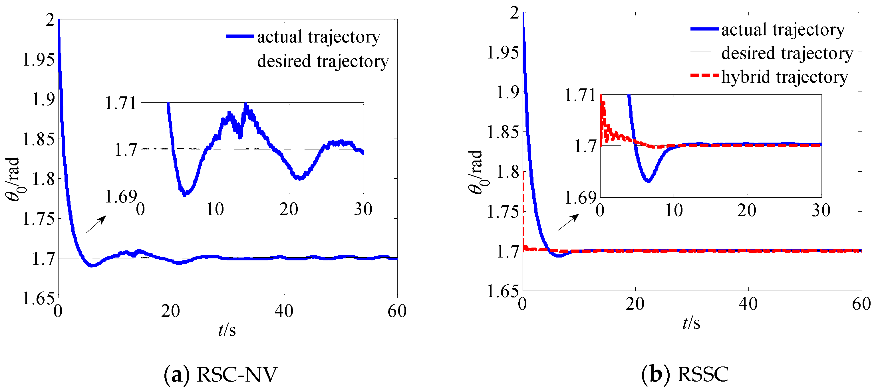
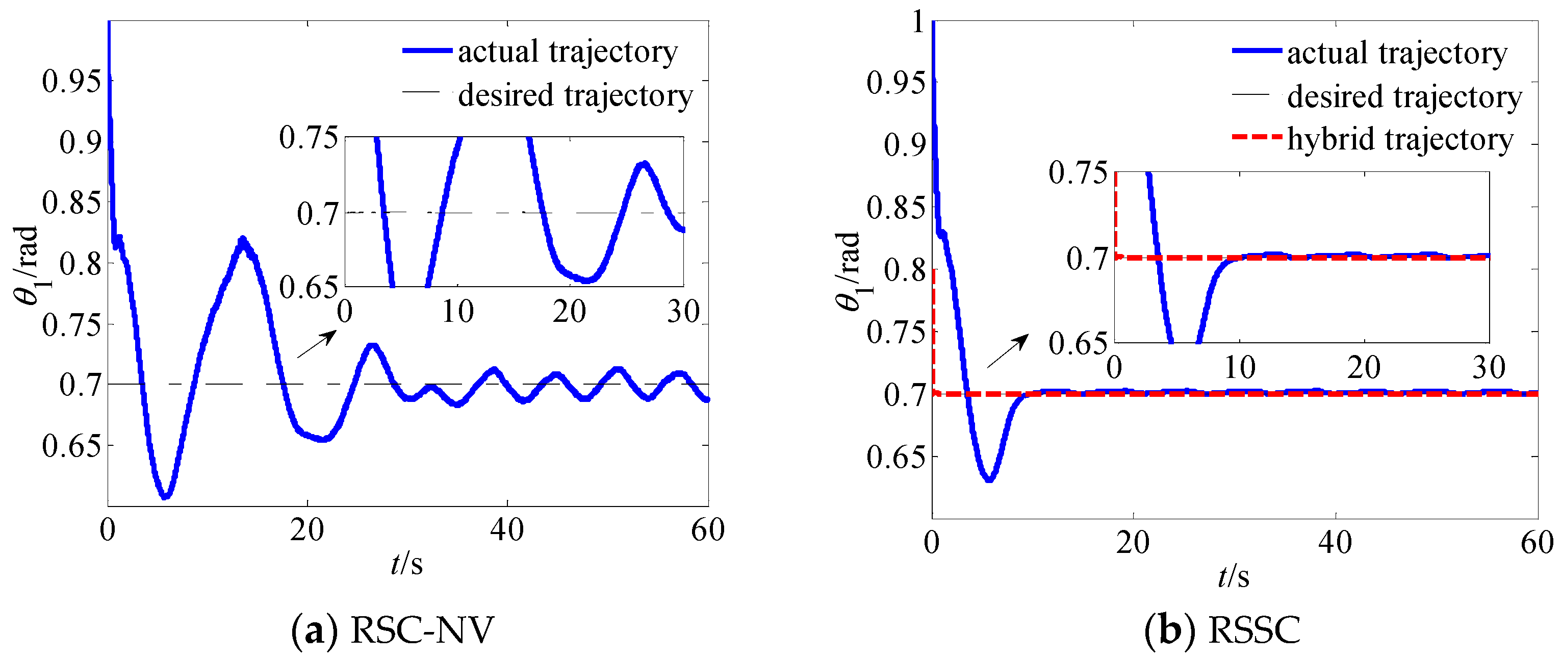
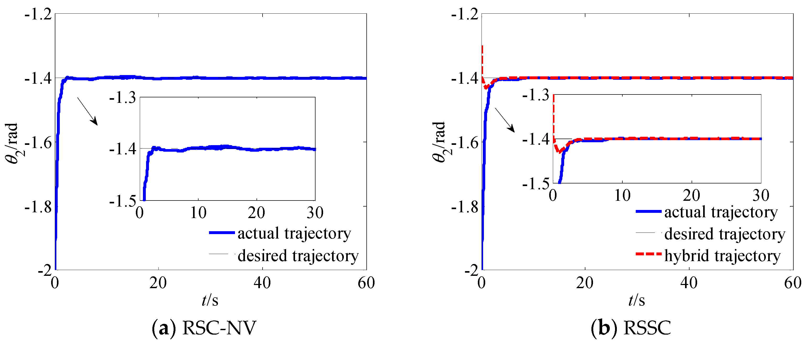
The trajectory tracking curves of the system base attitude under two control algorithms shown in Figure 2, Figure 3 and Figure 4 are the trajectory tracking curves of the system joint $O_1$ and joint $O_2$ under two control algorithms.

From Figure 2, Figure 3 and Figure 4, we can observe that the RSC-NV algorithm makes the base attitude and joint of the system stable in the desired trajectories. However, owing to the mutual coupling of the system motion and vibration, the uninhibited vibration of the base, links, and joints will lead to different amplitude vibrations of the base attitude and joint of the system, which will affect the control accuracy. Under the RSSC control algorithm, it can be seen that the convergence time of the base attitude stabilization and the tracking control of the joints is within 10 s. However, the convergence time under the RSC-NV algorithm is more than 30 s. The RSSC algorithm has a faster convergence speed than the RSC-NV algorithm. Therefore, the system has better control performance under the RSSC algorithm than the RSC-NV control method.

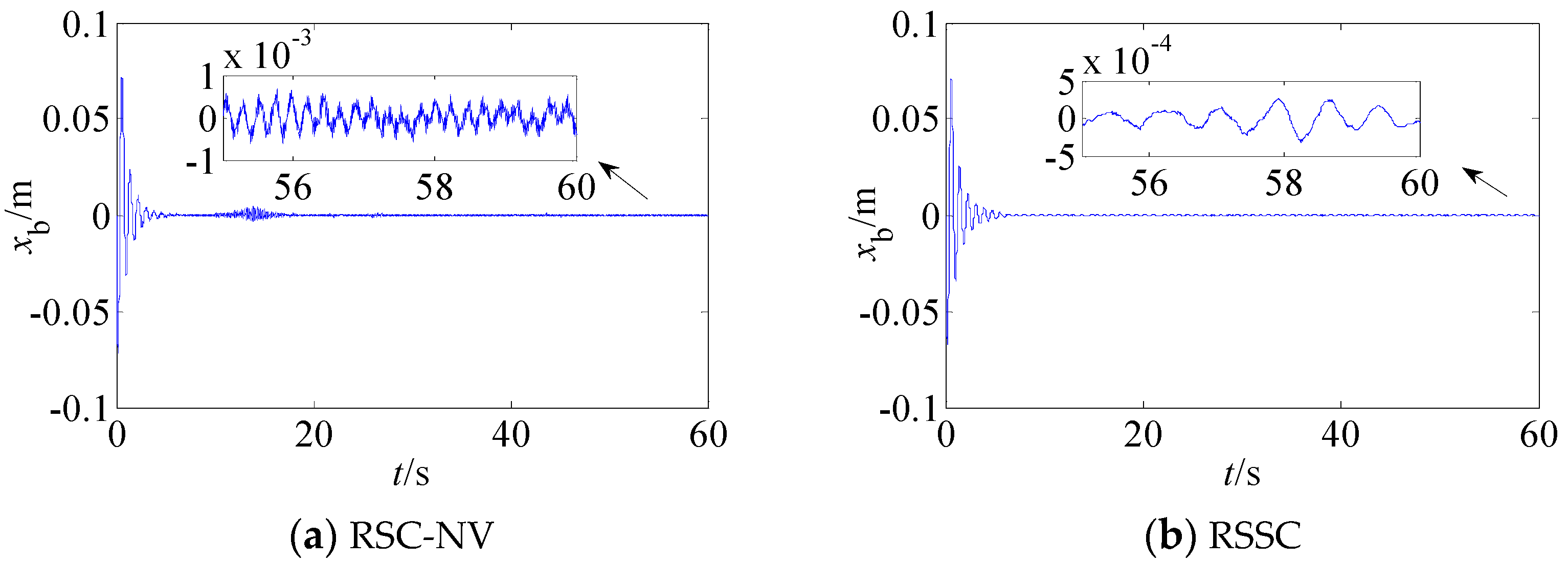
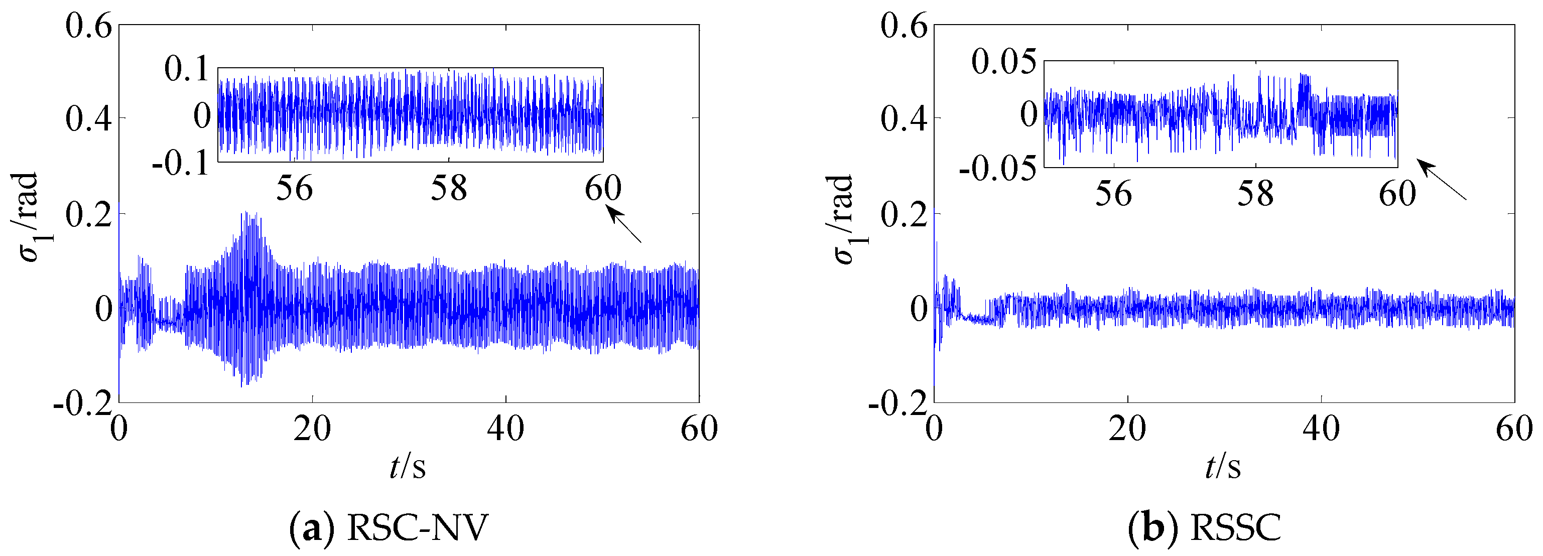
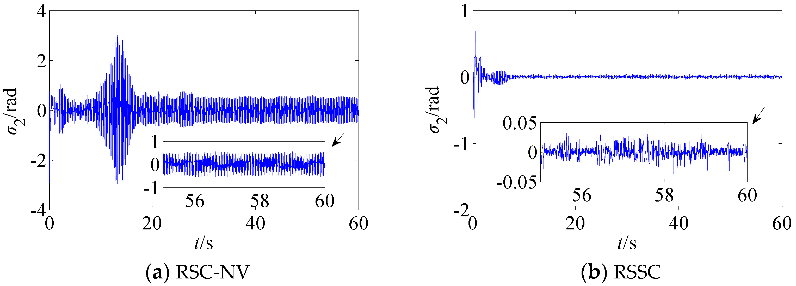
In order to show the effectiveness of the proposed algorithm for base and joint vibration suppression, the following simulation is carried out. Among them, Figure 5 shows the elastic vibration curves of the system base of under two control conditions, and Figure 6 and Figure 7 show the elastic vibration curves of joint $O_1$ and joint $O_2$ of the system under two control conditions.

From Figure 5, one can observe that the amplitude of the base is 1 mm under the RSC-NV algorithm. However, it can be seen that the base amplitude is 0.5 mm under the RSSC algorithm. The amplitude of joint $O_1$ is 0.1 rad under the RSC-NV algorithm, and the amplitude of joint $O_1$ is 0.05 rad under the RSSC algorithm, as show in Figure 6. Figure 7 shows that the amplitude of joint $O_2$ is 1 rad under the RSC-NV algorithm, the amplitude of joint $O_2$ is 0.05 rad under the RSSC algorithm. It is proved that the RSSC algorithm is effective at suppressing the vibration of the base and joints of the disturbed system.

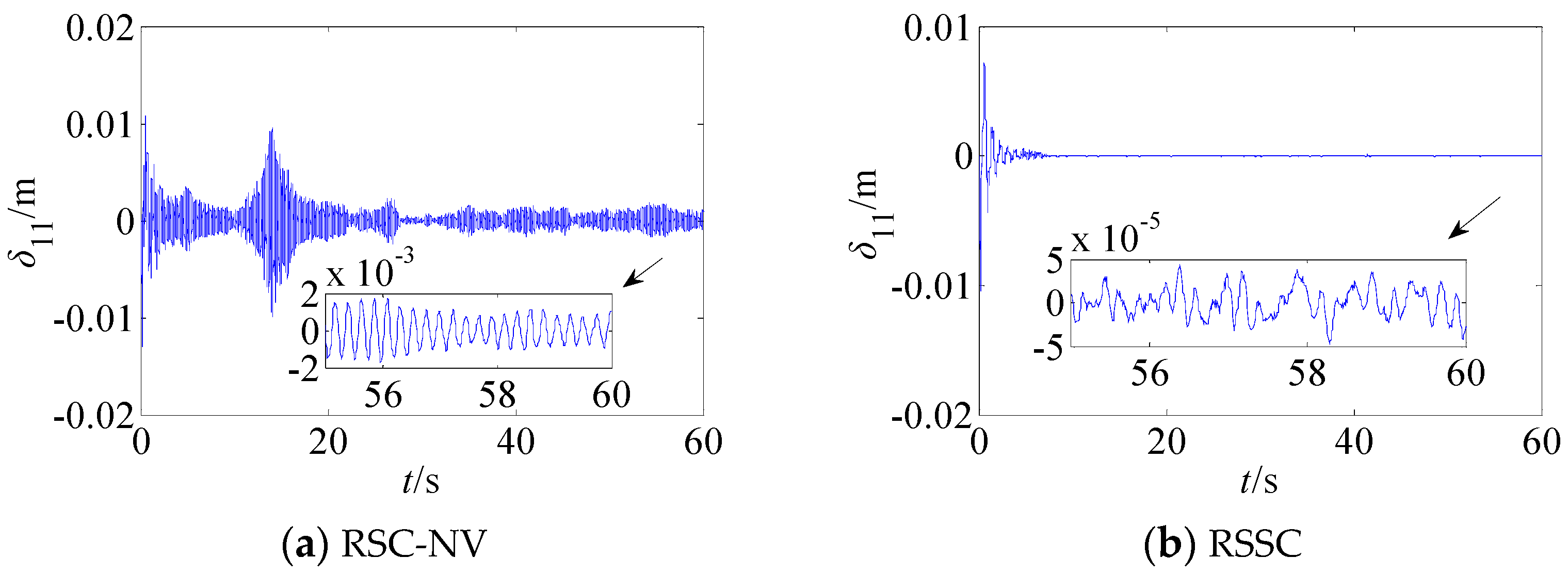
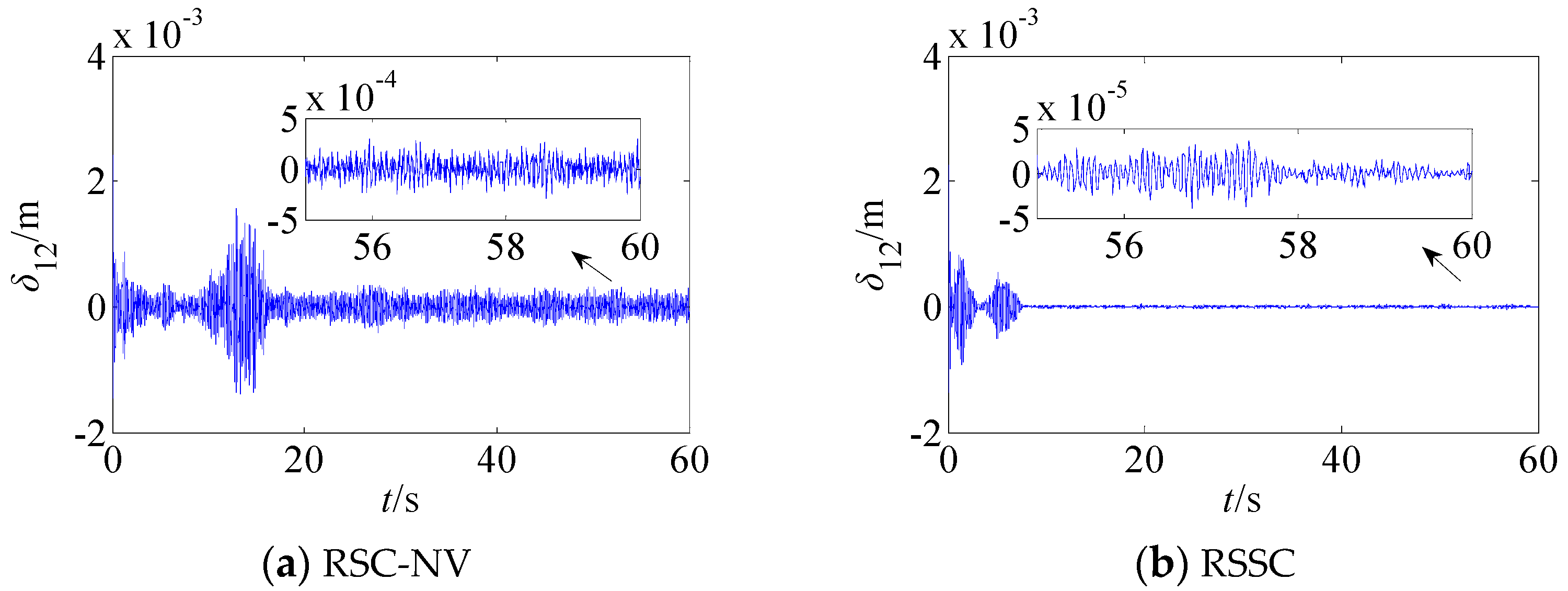
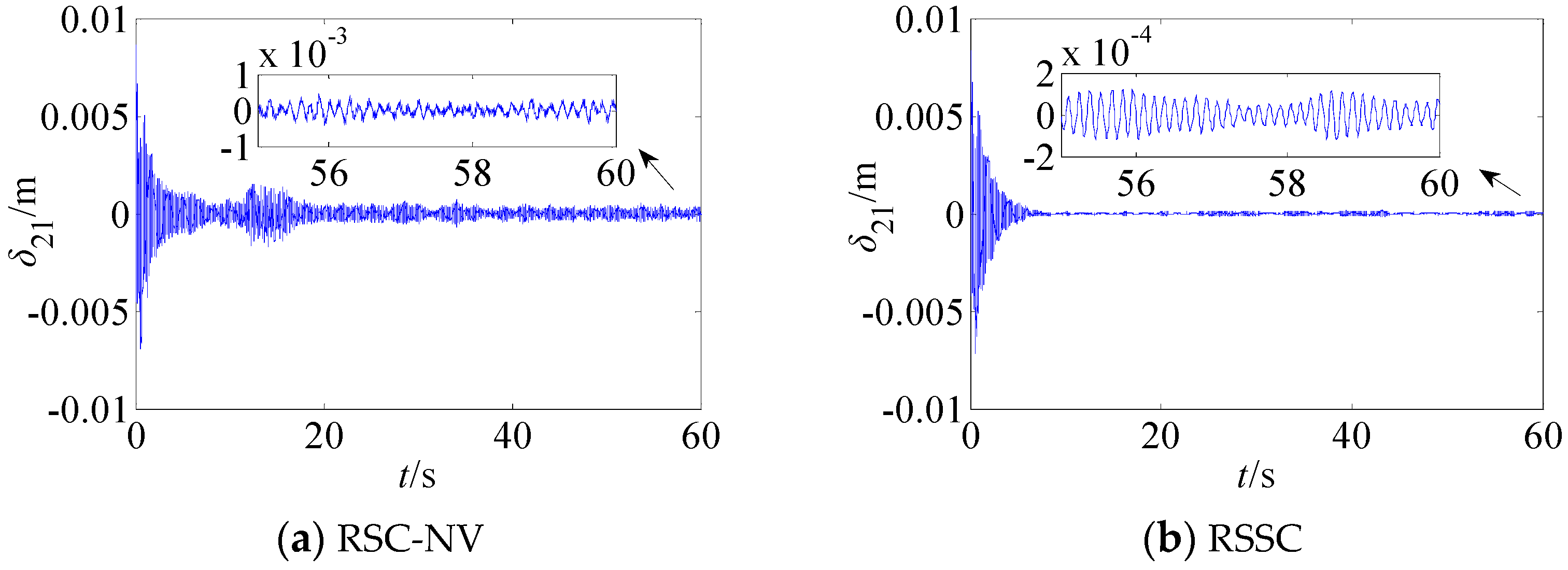
At the same time, the influence of the links vibration cannot be ignored. Figure 8 and Figure 9 show the first and second modal coordinates of flexible link $B_1$, respectively. Figure 10 and Figure 11 show the first and second modal coordinates of flexible link $B_2$.

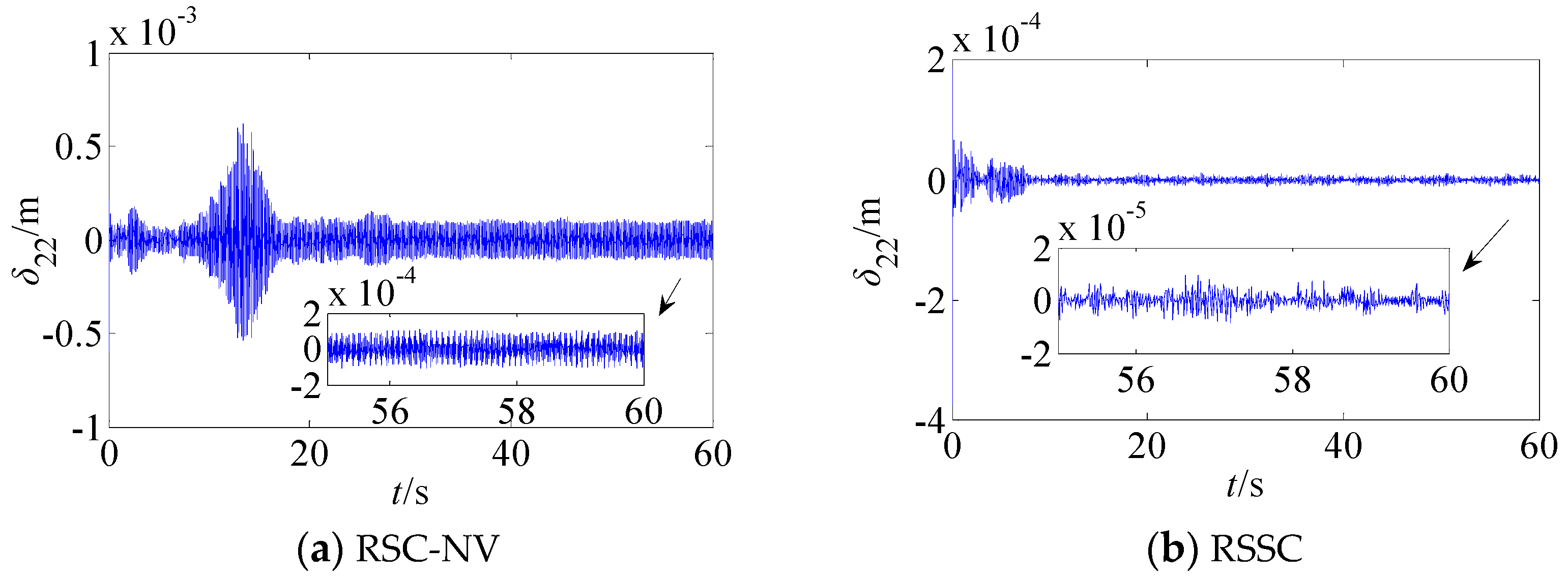
The first mode coordinates of the flexible link $B_1$ are 2 mm under the RSC-NV algorithm, and they are 0.05 mm under the RSSC algorithm, as depicted in Figure 8. Figure 9 shows that the second mode coordinates of the flexible link $B_1$ are 0.5 mm under the RSC-NV algorithm, and they are 0.05 mm under the RSSC algorithm. Meanwhile, from Figure 10, one can see that the first mode coordinates of the flexible link $B_2$ is 1 mm under the RSC-NV algorithm, and it is 0.2 mm under the RSSC algorithm. Figure 11 shows that the second mode coordinates of the flexible link $B_2$ is 0.2 mm under the RSC-NV algorithm, and it is 0.02 mm under the RSSC algorithm. All of the mode coordinates are obviously suppressed under the RSSC, which illustrates the effectiveness of the control schemes in the vibration suppression of system links.

7. Conclusions

The dynamic models of the fully flexible base–link–joint space robot and satellite were established by using the Lagrange equation and the Newton–Euler method, which provided the theoretical basis for the study of the capture process. With the help of the geometric position relationship and force transfer relationship between the contact points of the robot and the satellite, the impact effect on the collision was calculated, and the dynamic model of the system after capturing was established. Using the singular perturbation method, the system was decomposed into a slow subsystem (containing a base, joint rigid motion, and flexible link vibration) and a fast subsystem (containing a flexible base and joint vibration). A repetitive learning sliding mode controller based on the virtual force for the slow subsystem and an optimal controller for the fast subsystem were proposed. The simulation results show that the proposed control strategy can suppress the vibration of the disturbed system base attitude within 0.5 mm, the vibration of both joints within 0.05 rad, the first mode coordinates of both links within 0.2 mm, and the second mode coordinates of the two links within 0.05 and 0.02 mm, respectively. It can not only effectively suppress the elastic vibration of the base, joint and links of the system, but it can also realize the stable tracking of the desired signal through only one control input within 10 s.

References

1. Sands, T. Development of deterministic artificial intelligence for unmanned underwater vehicles (UUV). J. Mar. Sci. Eng. 2020, 8, 578. [Google Scholar] [CrossRef]
2. Ai, H.; Zhu, A.; Wang, J.; Yu, X.; Chen, L. Buffer compliance control of space robots capturing a non-cooperative spacecraft based on reinforcement learning. Appl. Sci. 2021, 11, 5783. [Google Scholar] [CrossRef]
3. Meng, Q.L.; Liang, J.X.; Ma, O. Identification of all the inertial parameters of a non-cooperative object in orbit. Aerosp. Sci. Technol. 2019, 91, 571–582. [Google Scholar] [CrossRef]
4. Cocuzza, S.; Pretto, I.; Debei, S. Least-Squares-Based Reaction Control of Space Manipulators. J. Guid. Control Dyn. 2012, 35, 976–986. [Google Scholar] [CrossRef]
5. Giordano, A.M.; Ott, C.; Albu, A. Coordinated control of spacecraft’s attitude and end-effector for space robots. IEEE Robot. Autom. Lett. 2019, 4, 2108–2115. [Google Scholar] [CrossRef]
6. Jin, R.; Rocco, P.; Geng, Y. Observer-based fixed-time tracking control for space robots in task space. Acta Astronaut. 2021, 184, 35–45. [Google Scholar] [CrossRef]
7. Evans, L. Canadian Space Robotics on Board the International Space. In Proceedings of the 2005 CCToMM Symposium on Mechanism, Machines, and Mechatronics, Montreal, QC, Canada, 26–27 May 2005; Canadian Space Agency: Montreal, QC, Canada, 2005; pp. 26–27. [Google Scholar]
8. Ramin, M.; Mojtaba, M. Maneuvering and vibrations control of a free-floating space robot with flexible arms. J. Dyn. Syst. Meas. Control 2011, 133, 051001. [Google Scholar]
9. Gorial, I. Sliding mode controller design for flexible joint robot. Eng. Technol. J. 2018, 36, 733–741. [Google Scholar]
10. Das, N.; Yip, M. Stochastic modeling of distance to collision for robot manipulators. IEEE Robot. Autom. Lett. 2021, 6, 207–214. [Google Scholar] [CrossRef]
11. Somov, Y.; Butyrin, S.; Somova, T.; Somov, S. Control of a free-flying robot at preparation for capturing a passive space vehicle. IFAC Pap. 2018, 51, 72–76. [Google Scholar] [CrossRef]
12. Wang, J.; Hyun, K.; Karam, D.; Lee, M.-C. Terminal sliding mode control with sliding perturbation observer for a hydraulic robot manipulator. IFAC-PapersOnLine 2018, 51, 7–12. [Google Scholar]
13. Madani, T.; Daachi, B.; Djouani, K. Modular-controller-design-based fast terminal sliding mode for articulated exoskeleton systems. IEEE Trans. Control Syst. Technol. 2017, 25, 1133–1140. [Google Scholar] [CrossRef]
14. Verrelli, C. A larger family of nonlinear systems for the repetitive learning control. Automatica 2016, 71, 38–43. [Google Scholar] [CrossRef]
15. Califano, F.; Bin, M.; Macchelli, A.; Melchiorri, C. Stability analysis of nonlinear repetitive control schemes. IEEE Control Syst. Lett. 2018, 2, 773–778. [Google Scholar] [CrossRef]
16. Kempf, C.; Messner, W.; Tornizuka, M.; Horowitz, R. Comparison of four discrete-time repetitive control algorithms. IEEE Control Syst. Mag. 1993, 13, 48–54. [Google Scholar]
17. Tomizuka, M.; Tsao, T.; Chew, I. Discrete-time domain analysis and synthesis of repetitive controllers. ASME J. Dyn. Syst. Meas. Contr. 1989, 3, 353–358. [Google Scholar] [CrossRef]
18. Yang, B.; Calise, A.; Craig, J. Adaptive output feedback control of a flexible base manipulator. J. Guid. Control Dyn. 2007, 30, 1068–1080. [Google Scholar] [CrossRef]
19. Yu, X.; Chen, L. Observer-based two-time scale robust control of free-flying flexible-joint space manipulators with external disturbances. Robotica 2017, 35, 2201–2217. [Google Scholar] [CrossRef]
20. Pradhan, S.K.; Subudhi, B. Real-time adaptive control of a flexible manipulator using reinforcement learning. IEEE Trans. Autom. Sci. Eng. 2012, 9, 237–249. [Google Scholar] [CrossRef]
21. Zhang, Q.; Liu, X.; Cai, G. Dynamics and control of a flexible-link flexible-joint space robot with joint friction. Int. J. Aeronaut. Space Sci. 2021, 22, 415–432. [Google Scholar] [CrossRef]
22. Yu, Y. Hybrid-trajectory based terminal sliding mode control of a flexible space manipulator with an elastic base. Robotica 2020, 38, 550–563. [Google Scholar] [CrossRef]
23. Wu, S.; Mou, F.; Liu, Q.; Cheng, J. Contact dynamics and control of a space robot capturing a tumbling object. Acta Astronaut. 2018, 151, 532–542. [Google Scholar] [CrossRef]
24. Zhao, X.; Xie, Z.; Yang, H.; Liu, J. Minimum base disturbance control of free-floating space robot during visual servoing pre-capturing process. Robotica 2020, 38, 652–668. [Google Scholar] [CrossRef]
25. Liu, Y.; Liu, X.; Cai, G.; Chen, J. Trajectory planning and coordination control of a space robot for detumbling a flexible tumbling target in post-capture phase. Multibody Syst. Dyn. 2021, 52, 281–311. [Google Scholar] [CrossRef]
26. Spong, M. Modeling and control of elastic joint robots. J. Dyn. Syst. Meas. Control 1987, 109, 310–319. [Google Scholar] [CrossRef]
27. Wang, M.; Sun, L.; Yin, W.; Dong, S.; Liu, J. Continuous robust control for series elastic actuator with unknown payload parameters and external disturbances. IEEE/CAA J. Autom. Sin. 2017, 4, 620–627. [Google Scholar] [CrossRef]
28. Kelly, R.; Santibanez, V.; Loria, A. Control of Robot Manipulators in Joint Space; Springer: London, UK, 2005. [Google Scholar]
29. Khalil, H. Nonlinear Systems, 3rd ed.; Prentice Hall: Englewood Cliffs, NJ, USA, 2002. [Google Scholar]
30. Lee, S.; Lee, C. Hybrid control scheme for robust tracking of two-link flexible manipulator. J. Intell. Robot. Syst. 2002, 34, 431–452. [Google Scholar] [CrossRef]
Figure 1. Structure of the flexible-base, flexible-joint and flexible-link space robot and the satellite.
Applsci 11 08077 g001
Figure 2. Trajectory tracking curve of the system base attitude.
Applsci 11 08077 g002
Figure 3. Trajectory tracking curve of the system joint O 1 .
Applsci 11 08077 g003
Figure 4. Trajectory tracking curve of the system joint O 2 .
Applsci 11 08077 g004
Figure 5. Elastic vibration curve of the system base.
Applsci 11 08077 g005
Figure 6. Elastic vibration curve of joint O 1 .
Applsci 11 08077 g006
Figure 7. Elastic vibration curve of joint O 2 .
Applsci 11 08077 g007
Figure 8. The first mode coordinates of the flexible link B 1 .
Applsci 11 08077 g008
Figure 9. The second mode coordinates of the flexible link B 1 .
Applsci 11 08077 g009
Figure 10. The first mode coordinates of the flexible link B 2 .
Applsci 11 08077 g010
Figure 11. The second mode coordinates of the flexible link B 2 .
Applsci 11 08077 g011
Publisher’s Note: MDPI stays neutral with regard to jurisdictional claims in published maps and institutional affiliations.