Frequency-Mixing Lasing Mode at European XFEL ^†

Abstract

We demonstrate generation of X-ray Free-Electron Laser (XFEL) pulses in frequency mixing mode at the SASE3 line of the European XFEL. The majority of the SASE3 FEL segments are tuned at two frequencies ${\omega }_1$ and ${\omega }_2$ following an alternate pattern. Leveraging on non-linearities generated through longitudinal dispersion in the system, we obtain electron bunching at a frequency difference ${\omega }_{FM}={\omega }_2-{\omega }_1$. FEL amplification at ${\omega }_{FM}$ follows in a few last radiator segments. We report on the generation of frequency mixing at photon energies between 500 eV and 1100 eV with pulse energies, depending on the length of the radiator, in the mJ level. This method allows generating low photon energies in cases where the FEL runs at high electron energy and the target photon energy cannot be reached in the main undulator, with the simple addition of a short, custom-made afterburner.

1. Introduction

Self-Amplified Spontaneous Emission (SASE) X-ray free-electron lasers (XFELs) generate beam energy and density modulation as well as output radiation by exploiting a narrow-bandwith FEL instability centered around a single resonant frequency. In other words, only a narrow spectral part of the input density modulation from the electron beam shot-noise is actually amplified around the resonant frequency.

As is well-known (see for example [1]), the FEL amplification process itself includes a non-linear regime, which follows the linear amplification down the undulator line. In the linear regime, different frequencies are treated fully independently. In the non-linear regime, this is no longer the case. This means that if the FEL amplification bandwidths were large enough, two separate frequencies ${\omega }_1$ and ${\omega }_2$ would also give rise to mixed frequency signals at ${\omega }_2\pm {\omega }_1$. In its standard configuration, the FEL bandwidth is very narrow and the relative spectrum is of order $2\rho$ at saturation, where $\rho$ indicates the efficiency parameter, so ${\omega }_1$ and ${\omega }_2$ are forced to be very near to each other, and the frequency mixing signals are outside of the amplification bandwith.

Nonetheless, a frequency mixing lasing mode can be obtained at facilities like the European XFEL where long, tunable undulators are available. In fact, if one tunes different undulator segments at two well-separated frequencies ${\omega }_1$ and ${\omega }_2$, both frequencies would be separately amplified in the linear regime, further yielding frequency mixing signals in the bunching at frequencies ${\omega }_2\pm {\omega }_1$, now within the reach in resonance frequency of a final radiator. The bunching at these two frequencies can be further optimized with the help of a downstream element adding longitudinal dispersion, which can be provided by a few detuned undulator segments. Pushing this scheme, the SASE FEL background from ${\omega }_1$ and ${\omega }_2$ can be kept at very low levels by keeping the first undulator segments (tuned at ${\omega }_1$ and ${\omega }_2$) in the linear regime, and relying on dispersion to obtain bunching at the mixed frequencies. Finally, as already anticipated above, the signal at the mixed frequencies can be picked up by a radiator tuned at the sum or at the difference frequency.

After a few introductory considerations in Section 2, in Section 3 we report about the generation of radiation in frequency mixing mode at the SASE3 undulator line of the European XFEL [2]. SASE3 [3] includes 21 undulator segments, each of them with a magnetic length of five meters, with tuneable K-parameter, and a period of 68 mm. In the experiments discussed here we focused on the generation of photon energies between 500 eV and 1100 eV, amplified by a few segments of SASE3. Frequency mixing is a well-known technique employed in radio- and laser-physics. It was considered for seeded FELs in [4,5], while in [6] frequency mixing of long-wavelength modulations of the electron beam induced by the laser heater and by the seed laser at FERMI was actually shown to generate FEL pulses in the Extreme ultraviolet (EUV) range. However, frequency mixing was never shown to work with SASE FELs, nor in the X-ray region. Besides constituting a novel method for the generation of XFEL radiation, as discussed in Section 4, frequency mixing may constitute a useful mode of operation, allowing to obtain target photon energies too low to be obtained in the main undulator, with the simple addition of a short afterburner with larger-than-baseline K parameter reach.

2. Theoretical Considerations about Frequency Mixing

As stated in the introduction, frequency mixing is enabled by nonlinearities in the FEL amplification process. As is well known, in the linear regime, bunching, energy modulation, and radiation at different frequencies evolve independently of each other, while in the non-linear regime this is no longer the case. However, pushing the FEL process to the non-linear regime to obtain frequency mixing has the disadvantage of a relatively large output at the initial frequencies ${\omega }_1$ and ${\omega }_2$, which spoils the electron beam. Moreover, ideally, one wants to control and keep the emission at ${\omega }_1$ and ${\omega }_2$ as small as possible because it constitutes usually unwanted background to the main pulse at the mixed frequency and, in particular, at the difference frequency ${\omega }_2-{\omega }_1$. This is achieved by keeping the FEL process at ${\omega }_1$ and ${\omega }_2$ in the linear regime, and mostly relying on a longitudinally dispersive region for creating non-linearities and optimizing the mixing process. Therefore, for the frequency-mixing setup at SASE3, we rely on configurations such as the one in Figure 1. The largest part of the setup is dedicated to the generation of electron energy modulation in the linear regime at two separate frequencies. This is obtained by using an alternating configuration where several undulator segments are tuned at frequency ${\omega }_1$, followed by others tuned at frequency ${\omega }_2$ (highlighted in green and yellow colors in the figure). In this way, diffraction effects are kept as small as possible and moreover, while one frequency is amplified, the beam energy modulation at the other can still benefit from the passage through a longitudinally dispersive medium. The exact sequence used in the configuration depends on the frequencies to be generated.

The first part of the undulator is followed by a second, consisting of a few segments that are detuned with respect to all the frequencies of interest. They act as a longitudinally dispersive region that further bunches the beam at the difference frequency ${\omega }_2-{\omega }_1$ (white region in Figure 1) by transforming energy modulation into density modulation. Finally, a few radiator segments are tuned to the difference frequency (orange region in Figure 1). Initially, the pre-bunched electron beam emits coherent radiation. However, if the radiator is longer than a gain length, FEL amplification takes place, resulting in an exponential increase of the frequency-mixed component of the radiation pulse.

We can describe the essence of the frequency mixing scheme outlined above for the simple case of vanishing small SASE bandwidths around ${\omega }_1$ and ${\omega }_2$ as a special subcase of the Echo Enable Harmonic Generation (EEHG) equation for the bunching factor [7]:

$$b_{n,m}=\left|e^{-(1/2){[n{B}_1+(Km+n)B_2]}^2}{J}_m[-(Km+n)A_2{B}_2]J_n\{-A_1[n{B}_1+(Km+n)B_2]\}\right|$$

(1)

Here, $b_{n,m}$ is the bunching at a harmonic with wave number $k_E=n{k}_1+m{k}_2$, with $k_{1,2}$ the wave numbers of the two EEHG lasers, $K=k_2/k_1$, $A_{1,2}=\Delta E_{1,2}/{\sigma }_E$, and $B_{1,2}=R_{56}^{1,2}{k}_1{\sigma }_E/E_0$. To describe the frequency-mixing mode, it is sufficient to consider a particularly simple case when $B_1=0$, i.e., the first chicane is turned off (the generalization to non-zero case is straightforward, and can be used to further optimize the performance). Moreover, our case of interest actually corresponds to $m=1$ and $n=-1$. Finally, setting $B=B_2$ we obtain the bunching factor at the mixed frequency [5].

$$b_{FM}=e^{-(1/2){\left[(K-1)B\right]}^2}{J}_1\left[(K-1)A_{2}B\right]J_1\left[(K-1)A_{1}B\right]$$

(2)

where we got rid of minus signs in the arguments and in the order of the Bessel functions since we consider modulus of the product. This bunching is then amplified in the output radiator. A thorough mathematical description of our system should actually include finite SASE bandwidths around the initial frequencies ${\omega }_1$ and ${\omega }_2$. However, such a description, as well as considerations on the statistics of the mixing process go beyond the scope of this paper, which is to report about experimental results instead. They will be developed in a separate, forthcoming work. Here we only limit ourselves to a few additional remarks.

First, we remind that in the linear regime, the SASE process can be modelled as a Gaussian process. Therefore, the arguments of the Bessel functions in Equation (2) must follow a Rayleigh distribution because they are proportional to the field amplitude through the energy modulations $A_1$ and $A_2$. As a result, $b_{FM}$ should be considered as a random variable too.

Second, we note that in the simple case of a cold beam, the exponential function in Equation (2) becomes unity. The probability density function for $b_{FM}$ can be easily obtained numerically by calculating the product of the Bessel functions in Equation (2). As their arguments, we use two large sets of independent random variates obtained from the Rayleigh distribution. The probability density function calculated in this way depends on the mean value (which we choose equal for both Rayleigh distributions). It is then straightforward to find the average value for $b_{FM}$ and to optimize it. We found that the maximum bunching amounts to about $20\%$ and is obtained for a mean value of $(K-1)A_{1,2}B\simeq 1.5$ slightly below the maximum of $J_1$, which is for $(K-1)A_{1,2}B\simeq 1.8$.

Finally, we note that while the SASE process in the linear regime follows Gaussian statistics, the frequency mixed signal obviously deviates from it, being the result of a non-linear operation.

3. Setup and Results

In the following, we report on several experimental results recently obtained at the SASE3 line of the European XFEL.

Table 1. Summary of the main parameters for four different freqeuncy mixing experiments (Exp. 1–4) at SASE3: photon energy of the target signal $E_{FM}$ and of the two frequencies $E_{2,1}$, electron energy $E_e$, radiation pulse energy after 1 up to n radiator segments $E_{r,1}\cdots E_{r,n}$. The values correspond to the actual signal $E_{FM}$, where the background due to the other colors has been substracted from the XGM reading. The comment (no) tap* means (no) tapering applied. Note that readings below 20–30 $\mathsf{\mu }$J are within the measurement uncertainty, and only serve as a rough estimation of the actual pulse energy.

Quantity	Exp. 1	Exp. 2	Exp. 3	Exp. 4
$E_{FM}$ (eV)	500	1100	700	500–600
$E_2$ (eV)	1200	2400	1600	1300–1400
$E_1$ (eV)	700	1300	900	800
$E_e$ (GeV)	11.5	16.5	14	11.5
$E_{r,1}$ ($\mathsf{\mu }$J)	-	10	-	-
$E_{r,2}$ ($\mathsf{\mu }$J)	30	40	40	20
$E_{r,3}$ ($\mathsf{\mu }$J)	150	180 (no tap*)	300	200
$E_{r,4}$ ($\mathsf{\mu }$J)	400	-	1100	1100
$E_{r,5}$ ($\mathsf{\mu }$J)	700 (no tap*)	-	2000 (no tap*)	2800
$E_{r,6}$ ($\mathsf{\mu }$J)	-	-	-	4500 (tap*)

summarizes the main parameters and output radiation pulse energy for the various experiments. In all cases, the bunch charge was 250 pC.

Since SASE3 has a period of 68 mm and consists of 21 variable-gap undulator segments, the total magnetic length amounts to 105 m [3]. After the 11th segment, a magnetic chicane for 2-color pump-probe (2CPP) experiments has been recently installed [8].

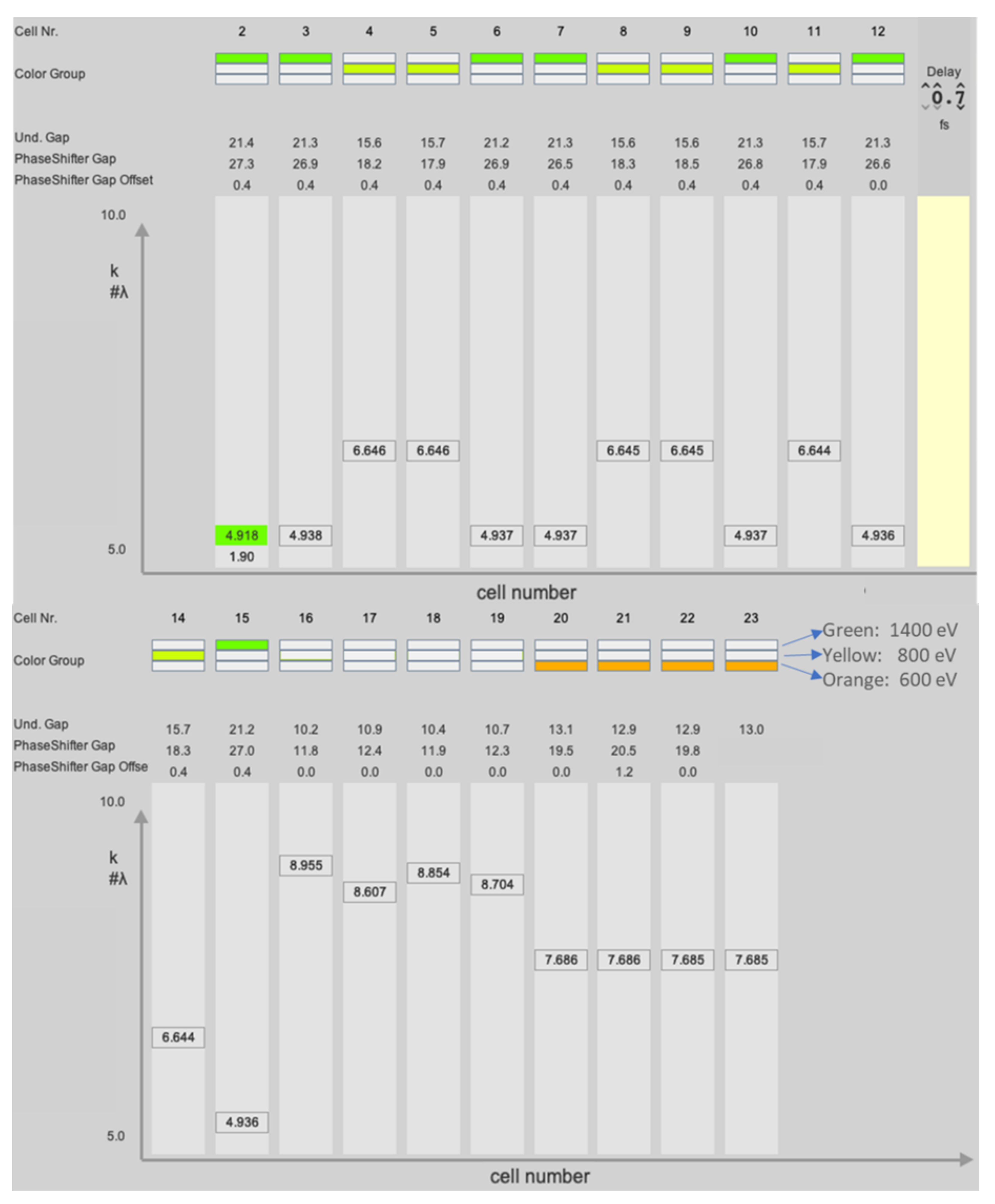
The undulator takes several hours to be configured and optimized for frequency mixing lasing, an operation that was carried out independently for the various experiments. However, once an optimal configuration file is saved, it can be loaded later on, within a few minutes. For the sake of illustration, Figure 1 shows one of the configurations used during the fourth experiment, Exp. 4 (see Table 1). The first part of the undulator comprises segments 2–15 (SASE3 begins from segment number 2 and segment number 13 corresponds to the 2CPP chicane) in an alternating sequence slightly favouring the second color at ${\omega }_2$ (equivalent to the photon energy $E_2=1400$ eV), as it corresponds to the shortest wavelength. Up to the present, it has not been not possible to keep the generation of ${\omega }_1$ and ${\omega }_2$ before the 2CPP chicane, which would have been optimal in terms of longitudinal dispersion control. However, we could still optimize the chicane to obtain some gain in the bunching. In the case shown in Figure 1, the optimum delay amounted to $0.7$ fs. Four segments (16–19) were used as dispersive elements with scrambled values of the K parameter optimized for optimum output, while the last four segments were tuned around 600 eV (the exact value was 604 for this case) with no taper applied. The actual values in the last line of Exp. 4 in Table 1 refer to a slightly different case of an optimum delay of $0.6$ fs, two segments (16–17) used as dispersive elements, and the last six segments, tapered, used as a radiator at the difference frequency.

A single X-ray Gas Monitor (XGM) device [9,10] could be used to investigate each color separately. This was achieved while suppressing the others by detuning or opening the relevant segments. We initially optimized the second color at 1400 eV in the first part of the undulator (up to segment 16) in normal SASE mode, removing every taper, and having care of avoiding saturation. After a first chicane delay optimization, which gave about a factor four increase in FEL output energy, we set the undulator segments into an alternating pattern configuration, taking care of obtaining a similar output from each separate color and keeping the output pulse energy level around a few tens of microjoules, to ensure that we were still in the linear regime. Later on, the configuration was tweaked a few times to optimize the output at ${\omega }_{FM}$ and to minimize the background colors at ${\omega }_{1,2}$. Figure 1 actually refers to an intermediate configuration. 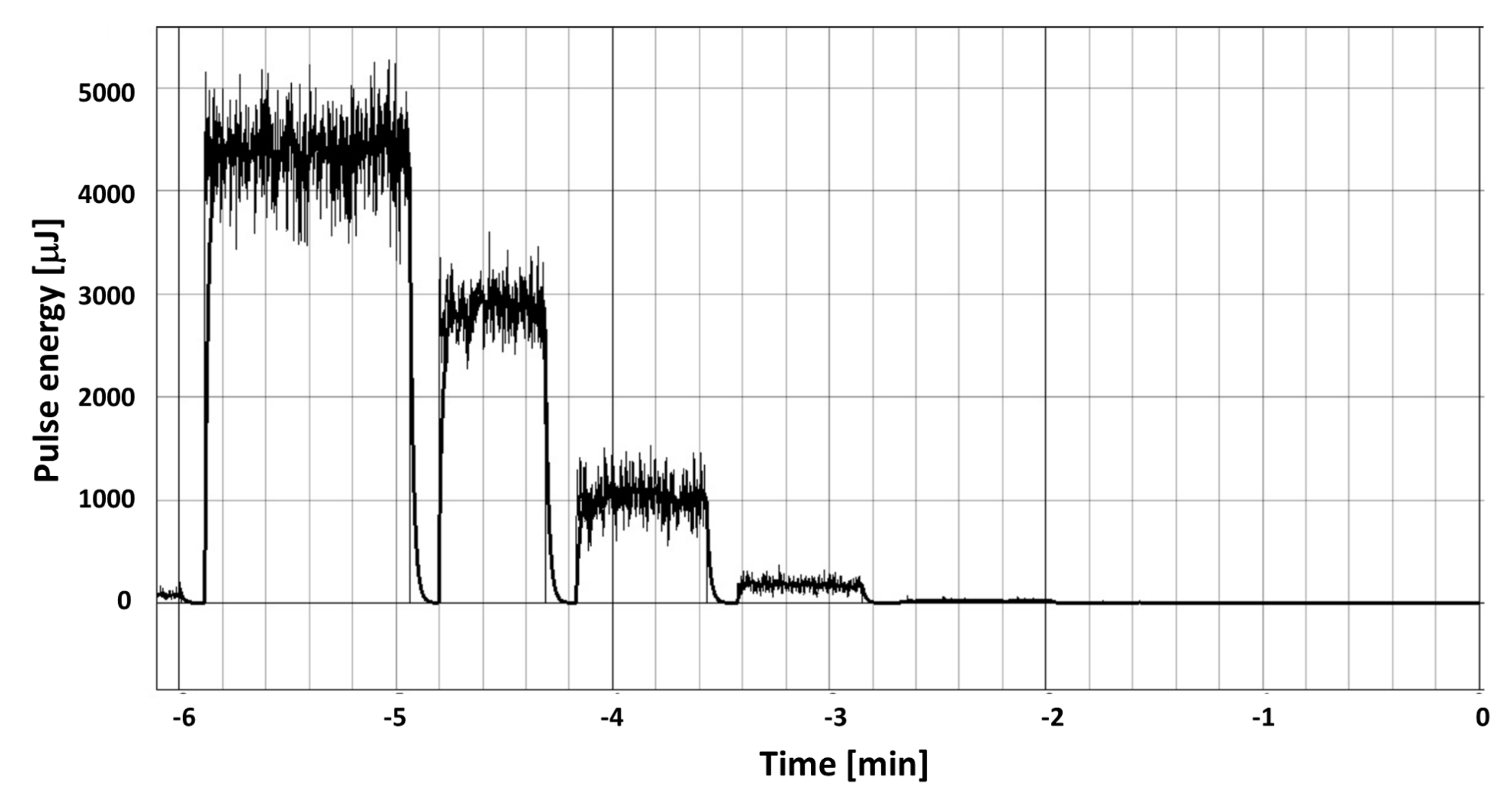At this point, calibrating the XGM for the difference frequency gives an unphysical background value from the colors at ${\omega }_1$ and ${\omega }_2$, but further closing a few segments (up to six) at the end of the undulator to the frequency difference ${\omega }_2-{\omega }_1$ (while keeping at least two segments detuned after segment 16 to create longitudnal dispersion), yields a variation in the XGM signal that corresponds directly to the pulse energy of the mixed frequency. Once the mixed frequency signal is found, one can follow up optimizing the configuration used and, subsequently, characterizing the output signal.

In Table 1, we report up to $4.5$ mJ with six radiator segments tuned at 600 eV. The segments in the radiator were tapered to an empirically found optimum valid for the six radiators. The XGM value of 4 $\mathsf{\mu }$J with one radiator segment closed was below the measurement uncertainty. Visually, it neared the background contribution of the two frequencies ${\omega }_{1,2}$ and since the XGM was set for ${\omega }_{FM}$ does not have physical meaning.

The backgrounds from each of the two colors ${\omega }_{1,2}$ were measured in the optimized configuration by detuning all other segments, and were found in the noise level (a few microjoules), which we ascertained separately by imparting a transverse kick to the electron trajectory prior to the entrance to SASE3. During the optimization, we were able to reduce the contribution of the two colors of about a factor ten (from the few tens of microjoules reported above), while providing an optimal bunching level at ${\omega }_{FM}$. 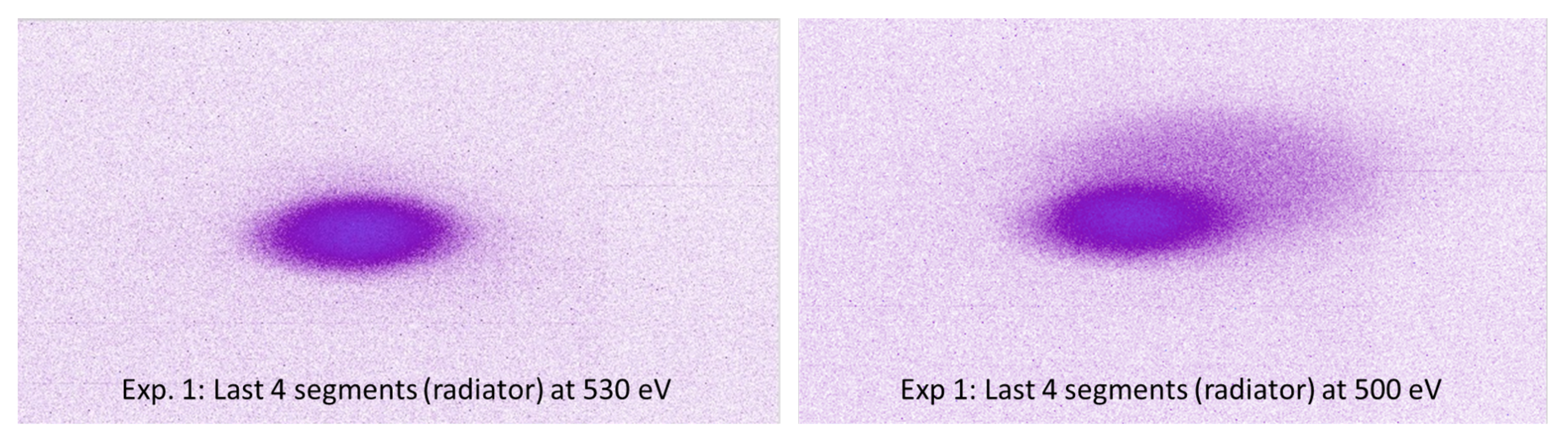In this respect, tuning the longitudinal dispersion by adjusting the K value of the segments out of resonance before the final radiator easily led to important changes during the tuning process (without performing a systematic study, we found a factor two improvement with four radiator segments). Note that the background level decreased substantially in time as we performed the various experiments. During the very first experiment, Exp. 1 (see Table 1), we imaged [11] the transverse FEL radiation pulse distribution with the help of a scintillator with the radiator segments detuned (left plot in Figure 2) or at resonance with the mixed frequency (right plot in Figure 2). The appearance of the freqeuncy mixed signal, with a slight pointing difference with respect to the background from the two initial colors at 1200 eV and 700 eV is evident. The estimated angular divergence at 500 eV is in the order of 20 $\mathsf{\mu }$rad.

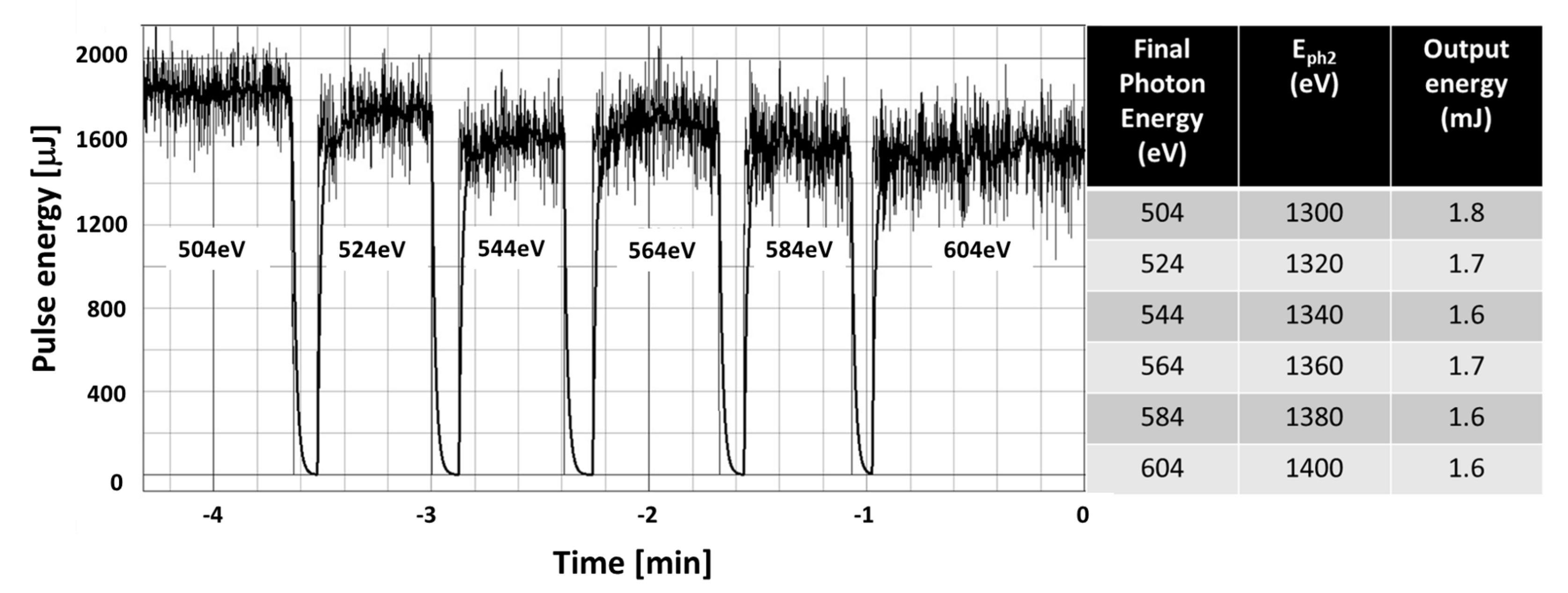
An important feature of the frequency mixed mode is that, despite the more involved setting procedure, it is easily tuneable in output photon energy. We showed this during the fourth experiment, by scanning the final photon energy from 504 eV to 604 eV in steps of 20 eV. This was done by adjusting the K parameter of the final radiator (and hence ${\omega }_{FM}$) and that of the color with highest photon energy, ${\omega }_2$. The scan was performed with four radiator segments tuned at resonance and without adjusting any other parameter. It took about four minutes to perform this scan manually and it could be easily automatized. Results are shown in Figure 3, which shows an average output pulse energy stability within about 200 $\mathsf{\mu }$J.

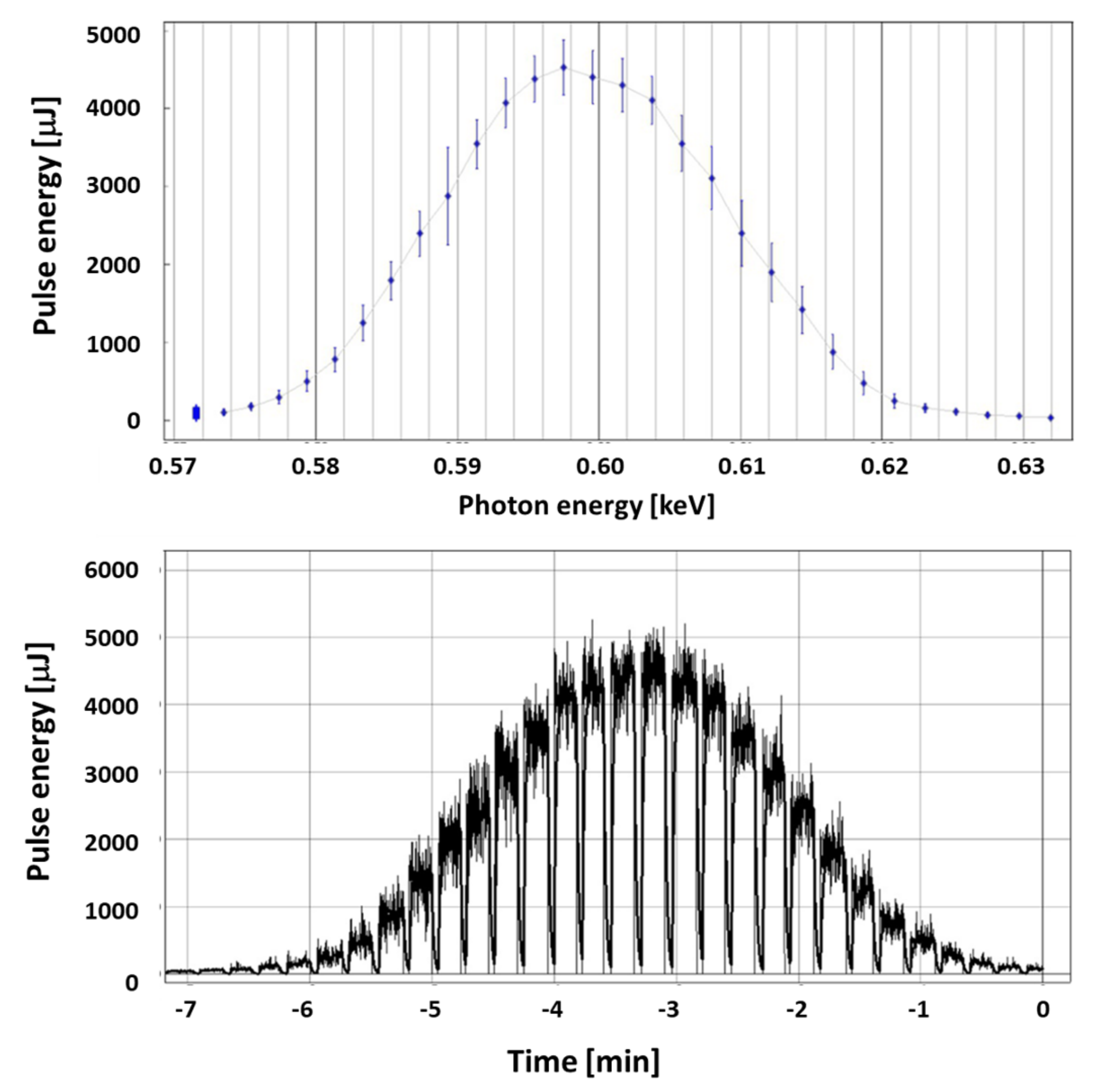
Another important characteristic to be studied is the amplification bandwidth around the nominal output frequency ${\omega }_{FM}$. This can be done by correlating the pulse energies measured by the XGM with the photon energy, that is by scanning the K parameter of the radiator segments. The results of the scan are presented in the upper plot in Figure 4, where each measure is found by averaging each point over 40 measures (4 s at 10 Hz). The lower plot in the same figure shows the actual pulse energies during the scan.

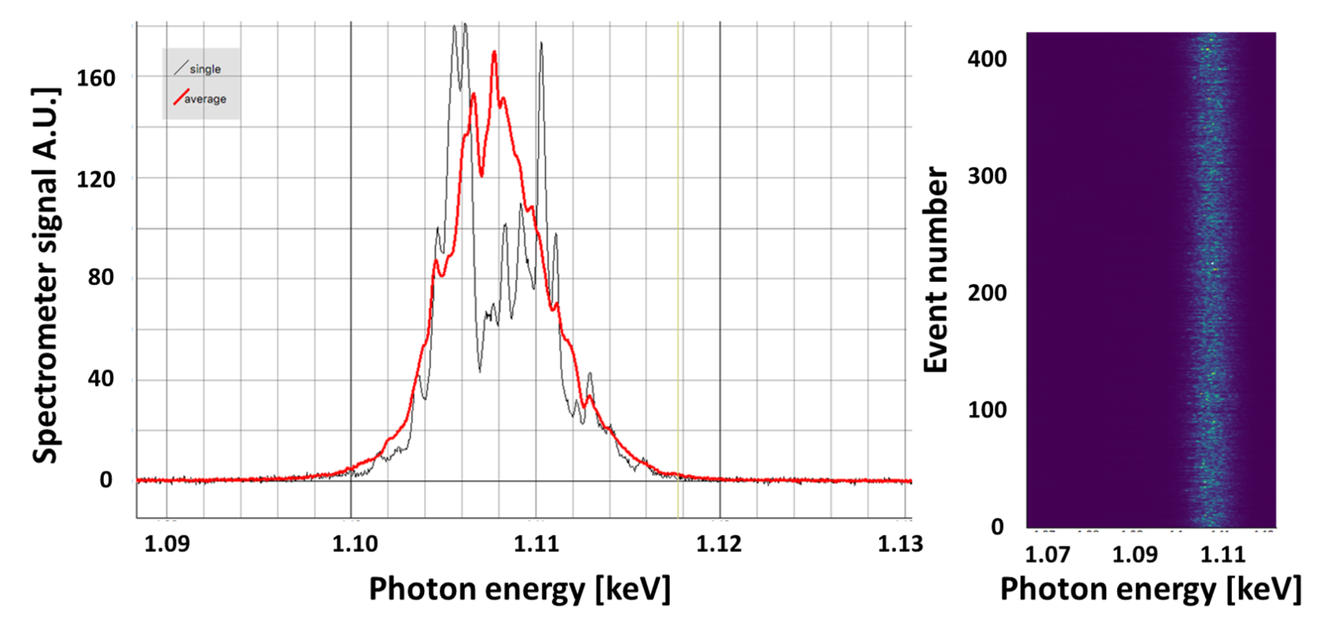
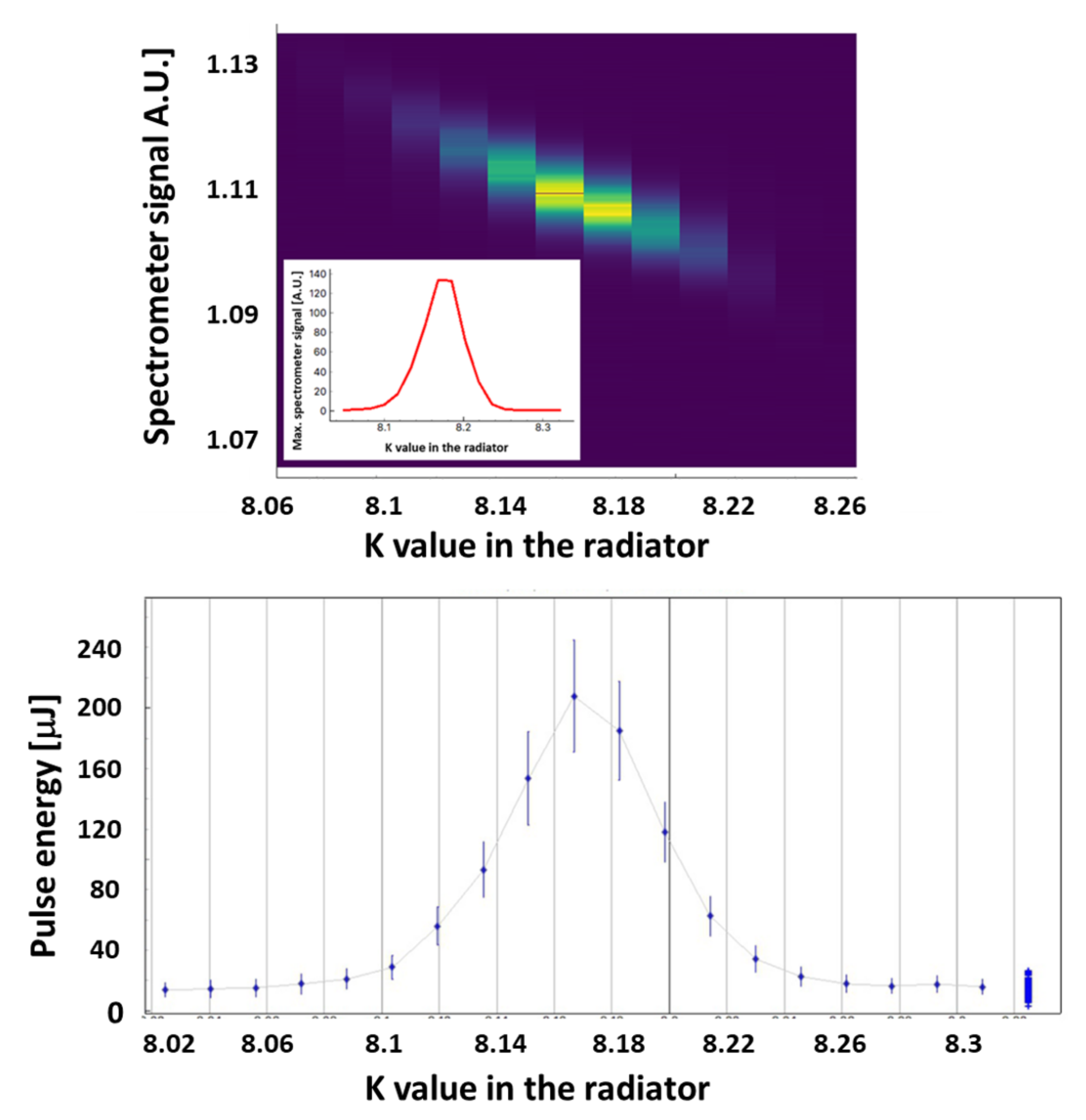
It should be remarked that the bandwidth provided by this scan does not correspond directly to the bandwidth of the output radiation. To illustrate this point, during one of the various experiments, Exp. 2 (see Table 1), we resolved the frequency-mixed signal in frequency with the help of a spectrometer [12]; see Figure 5. The figure corresponds to the case of three closed radiator segments. In Figure 6, upper plot, we show the color-coded spectra as a function of the K parameter: in the inset we extract the same information as in a K-parameter scan done with the pulse energies measured by the XGM (see Figure 6, lower plot). Note that the FWHM bandwidth is about $0.6\%$, which is larger than intrinsic bandwidth of SASE at this photon energy, but is comparable to the typical performance of SASE3 that is usually strongly influenced by electron energy chirp.

4. Outlook and Conclusions

In this paper, we investigated frequency mixing generation at the SASE3 line of the European XFEL. We implemented it by using the first part of SASE3 to generate two frequencies ${\omega }_1$ and ${\omega }_2$ in alternating K configuration, by subsequently obtaining a large bunching at ${\omega }_2-{\omega }_1$ using a few non-resonant segments as dispersive elements and finally by generating radiation at the target frequency in a last, short part of SASE3 used as a radiator; see Figure 1. We demonstrated, for the first time, freqeuncy mixing in the X-ray region, between 500 eV and 1100 eV. We showed that the bunching can be amplified in the radiator, and that six SASE3 segments dedicated to amplification allow reaching $4.5$ mJ at 500–600 eV, see Table 1 and Figure 7. We studied the actual amplification bandwidth by means of K-parameter scans in the radiator; see Figure 4. Finally, we demonstrated easy tuneability over a range of 100 eV (see Figure 3) and showed that the frequency mixing mode of operation only needs a single XGM in order to be established and operated. Nevertheless, in some of the experiments we also acquired spectra, see Figure 5 and Figure 6, and transverse profile distribution, see Figure 7 of the frequency mixed signal.

It should be noted that together with the bunching at the difference frequency ${\omega }_2-{\omega }_1$ one automatically generates bunching at the sum frequency ${\omega }_2+{\omega }_1$ as well. The sum frequency generation is certainly an interesting phenomenon to consider, and it might be useful to reach shorter wavelengths than allowed by the baseline mode of operation of an FEL when a suitable radiator is available. However, in this study we limited ourselves to the difference frequency generation.

This is not only of interest as a phenomenon pertaining FEL physics, but has the practical relevance of a method to provide low photon energies for operation at high electron energies. In fact, due to constraints posed by the parallel operation of three FEL lines (SASE1 and SASE2, enabling hard X-rays and SASE3, in the soft X-rays range), it is usually preferred to operate the accelerator at relatively high electron energies. To be specific, European XFEL usually operates with an electron energy of 14 GeV and a charge of 250 pC. For this electron energy, the lowest photon energy in the SASE3 undulator is 660 eV. This is limited by the maximum value of the undulator parameter $K\simeq 9$, with a period of $6.8$ cm. The generation of pulses with lower photon energy is possible, but only at lower electron energies, which poses issues in the planning of simultaneous experimental activities at SASE1, SASE2, and SASE3. Consider now the addition of a short radiator reaching lower photon energies than those achievable by the main FEL undulator at the fundamental and at a fixed electron energy. Using a such radiator, frequency mixing allows generating intense FEL pulses at lower photon energies than those permitted in standard SASE mode. This offers an interesting alternative for operating the facility at the same time for very soft and very hard x-ray radiation using a single electron energy.

An Apple-X afterburner made of four segments with 22 periods each and a period length of 9 cm will soon be installed after the main SASE3 undulator. At 14 GeV, it will allow to be resonant down to 440 eV in circular or linear horizontal/vertical polarization mode. Therefore, one can use the frequency mixing mode to generate bunching between 440 eV and 660 eV in the main SASE3 undulator, as difference of allowed energies, and subsequently exploit the Apple-X afterburner to actually radiate at those photon energies. One cannot directly compare the output of our experiment and the actual output for the frequency mixing mode enabled by the Apple-X afterburner, because of the different parameters (undulator period, photon energy, electron energy, and undulator polarization). Nevertheless, theoretically, for the same parameters of the electron beam the gain length for 300 eV and a period of 9 cm is comparable with that for 700 eV and a period od 6.8 cm. This reasoning suggests that the four Apple-X afterburner segments will be roughly equivalent to two SASE3 baseline segments. For two SASE3 segments used as radiators, Table 1 indicates an output of only a few tens of microjoules, beacause we report the gain of a setup optimized for six radiators. However, during the same experiment, we were able to obtain up to 200 $\mathsf{\mu }$J with two segments, just by optimizing the longitudinal dispersion.

Moreover, this energy level can be dramatically boosted by possibly refurbishing a few SASE3 undulator segments, increasing their period to 9 cm, which is a possibility under current scrutiny at the European XFEL. In other words, frequency mixing allows generating X-ray pulses for an FEL running at high electron energy where the target photon energy is too low to be reached in the main undulator, with the simple addition of a short afterburner with extended photon energy reach.