
Integration of Functional Link Neural Networks into a Parameter Estimation Methodology

1
Department of Electrical Engineering, Faculty of Engineering and Technology, Quy Nhon University, Quy Nhon 591417, Vietnam
2
Department of Industrial & Management Systems Engineering, Dong-A University, Busan 49315, Korea
3
Maritime Safety and Environmental Research Division, Korea Research Institute of Ships & Ocean Engineering, Daejeon 34103, Korea
4
Department of Technology Management Engineering, Jeonju University, Jeonju 55069, Korea
*
Authors to whom correspondence should be addressed.
Appl. Sci. 2021, 11(19), 9178; https://0-doi-org.brum.beds.ac.uk/10.3390/app11199178
Submission received: 31 July 2021
/
Revised: 7 September 2021
/
Accepted: 17 September 2021
/
Published: 2 October 2021
(This article belongs to the Special Issue 2021 Smart Manufacturing on Production System, Quality Assurance, Process Optimization, and Digital Modeling)
Abstract
:In the field of robust design, most estimation methods for output responses of input factors are based on the response surface methodology (RSM), which makes several assumptions regarding the input data. However, these assumptions may not consistently hold in real-world industrial problems. Recent studies using artificial neural networks (ANNs) indicate that input–output relationships can be effectively estimated without the assumptions mentioned above. The primary objective of this research is to generate a new, robust design dual-response estimation method based on ANNs. First, a second-order functional-link-NN-based robust design estimation approach has been proposed for the process mean and standard deviation (i.e., the dual-response model). Second, the optimal structure of the proposed network is defined based on the Bayesian information criterion. Finally, the estimated response functions of the proposed functional-link-NN-based estimation method are applied and compared with that obtained using the conventional least squares method (LSM)-based RSM. The numerical example results imply that the proposed functional-link-NN-based dual-response robust design estimation model can provide more effective optimal solutions than the LSM-based RSM, according to the expected quality loss criteria.
1. Introduction
Over the past two decades, robust parameter design (RPD), also known as robust design (RD), has been widely applied to improve the quality of products in the offline stage of practical manufacturing processes. Bendell et al. [1] and Dehnad [2] discussed the applications of RD to various engineering concerns in the process, automobile, information technology, and plastic technology industries. The primary purpose of RD is to obtain the optimal settings of control factors by minimizing the process variability and deviation based on the mean value and the presupposed target, which are often referred to as the process bias. As Taguchi explored [3], RD includes two main stages: design of experiments and two-step modeling. However, orthogonal arrays, statistical analyses, and signal-to-noise ratios used in conventional techniques to solve RD problems have been questioned by engineers and statisticians, such as León et al. [4], Box [5], Box et al. [6], and Nair et al. [7]. As a result, to resolve these shortcomings, several advanced studies have been proposed.
The most significant alternative to Taguchi’s approach is the dual-response model approach based on the response surface methodology (RSM) [8]. In this approach, the process mean and variance (or standard deviations) are approximated as two separate functions of input factors based on the LSM. In addition, the dual-response model approach provides an RD optimization model that minimizes the process variability while the process mean is assigned equal to the target value. However, the dual-response approach in Vining and Myers [8] may not always provide efficient optimal RD solutions, which have been discussed in Del Castillo and Montgomery [9] and Copeland and Nelson [10]. Instead, they employed the standard nonlinear programming techniques of the generalized reduced gradient method and the Nelder–Mead simplex method to provide better RD solutions. Subsequently, Lin and Tu [11] identified a drawback in the dual-response model approach whereby the process bias and variance are not simultaneously minimized. To overcome this issue, they proposed a mean square error (MSE) model.
The RSM comprises statistical and mathematical techniques to develop, improve, and optimize processes. It helps design, develop, and formulate new products, as well as improve the existing product designs [12]. The unidentified relationship between input factors and output responses can be investigated using the RSM. To define the input–output functional relationship, the conventional LSM is used to estimate unknown model coefficients. The LSM-based RSM assumes that the sample data follow a normal distribution, and the error terms hold a fixed variance with zero mean. Unfortunately, the Gauss–Markov theorem is not applicable in several practical situations, which implies that those assumptions are not valid. Therefore, weighted least squares, maximum likelihood estimation (MLE), and Bayesian estimation methods can be used as alternatives to determine model parameters. Pertaining to MLE, the unknown parameters are considered as constant, and the observed data are treated as random variables [13]. The MLE approach with abnormal distributed data was implemented in Lee and Park [14], Cho et al. [15], and Cho and Shin [16], whereas Luner [17] and Cho and Park [18] proposed the weighted least squares methods to estimate the model coefficients in the case of unbalanced data. Most estimation methods based on the RSM consider several assumptions or require specific data types to determine functions between the process mean or variance and input factors.
Over the past two decades, artificial neural networks (ANNs), often known as neural networks (NNs), have been widely used to classify, cluster, approximate, forecast, and optimize datasets in the fields of biology, medicine, industrial engineering, control engineering, software engineering, environmental science, economics, and sociology. An ANN is a quantitative numerical model that originates from the organization and operation of the neural networks of the biological brain. The basic building blocks of every ANN are artificial neurons, i.e., simple mathematical models (functions). Typical ANNs comprise thousands or millions of artificial neurons (i.e., nonlinear processing units) connected via (synaptic) weights. ANNs can “learn” a task by adjusting these weights. Neurons receive inputs with their associated weights, transform those inputs using activation functions, and pass the transformed information as outputs. It has been theoretically proved that ANNs can approximate any continuous mapping to arbitrary precision without any assumptions [19,20,21,22]. Furthermore, without any knowledge of underlying principles, ANNs can determine unknown interactions between the input and output performances of a process because of their data-driven and self-adaptive properties. Accordingly, the functional correlation between the input and output quality characteristics in RD can be modeled and analyzed by NNs without any assumptions. The integration of an NN into the experiment design procedure of an RD model has been mentioned in Rowlands et al. [23] and Shin et al. [24]. In recent times, Arungpadang and Kim [25] presented a feed-forward NN-based RSM that improved the precision of estimations without additional experiments. Le et al. [26] proposed an NN-based estimation method that identified a new screening procedure to determine the optimum transfer function, so that a more accurate solution can be obtained. A genetic algorithm with NNs has been executed in Su and Hsieh [27], Cook et al. [28], Chow et al. [29], Chang [30], Chang and Chen [31], Arungpadang et al. [32], and Villa-Murillo et al. [33] as an estimation method to investigate the optimal quality characteristics with associated control factor settings in the RD model without the use of estimation formulas. Winiczenko et al. [34] introduced an efficient optimization method by combining the RSM and a genetic algorithm (GA) to find the optimal topology of ANNs for predicting color changes in rehydrated apple cubes.
Therefore, the main objective is to propose a new dual-response estimation approach based on NNs. First, the normal quadratic process mean and standard deviation functions in RD are estimated using the proposed functional-link-NN-based estimation method. Second, the Bayesian information criterion (BIC) is used to quantify the magnitude of neurons in the hidden layer, which affects the coefficients in the estimated input–output equations. Finally, the results of the case study are presented to verify the effectiveness of the proposed NN-based estimation method compared with the LSM-based RSM. The graphical overview of the proposed NN-based estimation method is demonstrated in Figure 1.
The remainder of the study is organized as follows: Section 2 introduces the conventional LSM-based RSM. Section 3 describes the functional-link-NN-based dual-response estimation model. Section 4 explains the outputs generated by the proposed NN-based estimation method and analyzes the LSM-based RSM based on the results of the case study. Finally, Section 5 concludes the study and describes further studies.
2. Conventional LSM-Based RSM
The RSM was first introduced by Box and Wilson [35] and is used to model empirical relationships between output and input variables. Myers [36] and Khuri and Mukhopadhyay [37] present insightful commentaries on the different development phases of the RSM. When the exact functional relationship is very complicated or is unknown, the conventional LSM is used to estimate the input–response functional relationships of the output [38,39]. In general, the estimated second-order response surface functions are used to analyze RD problems. The estimated process mean and standard deviation functions proposed by Vining and Myers [8] can be defined as follows:
where is a vector of input variables, and and are the estimated coefficients in the mean and standard deviation functions, respectively. These regression coefficients can be estimated using the LSM as
where is the design matrix of control factors, and and are the mean and standard deviation of the observed responses, respectively.
3. Proposed Dual-Response Model Based on Functional Link NNs
3.1. Proposed Functional Link NN
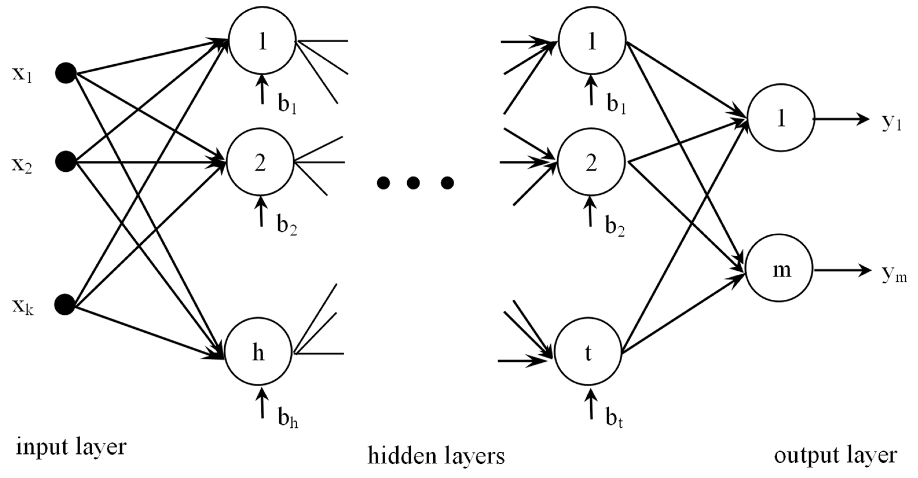
ANNs are comprised of various processing elements known as artificial neurons or nodes, which are interconnected. Each neuron obtains input signals from the previous nodes, aggregates these signals with the related weights, and generates output signals through a transfer function (or activation function). This output signal forms the input signal for other nodes. The multilayer feed-forward back-propagation NN is the most influential model applied to various practical problems. A multilayer feed-forward back-propagation NN model comprises several layers; each layer contains several nodes. The first and last layers inside the network are considered as input and output layers, respectively, as the input and output units in the NN system are involved. Various hidden layers are located between the input and output layers. A multilayer feed-forward back-propagation NN comprises one input layer, one output layer, and various hidden layers between the input and output layer. The overall structure of a multilayer feed-forward back-propagation NN is illustrated in Figure 2.
The universal approximation theorem for multilayer feed-forward networks was proposed by Cybenko [21] and Hornik et al. [20]. A multilayer feed-forward NN with a hidden layer can approximate a multidimensional, continuous, and arbitrary nonlinear function with any desired accuracy, as mentioned in Funahashi [22] and Hartman et al. [40], based on the theorem stated by Hornik et al. [20] and Cybenko [21]. In the hidden area, the transfer function is used to figure out the functional formation between the input and output factors. Popular transfer functions used in ANNs include step-like, hard limit, sigmoidal, tan sigmoid, log sigmoid, hyperbolic tangent sigmoid, linear, radial basis, saturating linear, multivariate, softmax, competitive, symmetric saturating linear, universal, generalized universal, and triangular basis transfer functions [41,42]. In RD, there are two characteristics of the output responses that are of particular interest: the mean and standard deviation. Each output performance can be separately analyzed and computed in a single NN structure based on the dual-response estimation framework. Figure 3 illustrates the proposed functional-link-NN-based dual-response estimation approach.
As shown in Figure 3, denote control variables in the input layer. The weighted sum of the factors with their corresponding biases can represent the input for each hidden neuron. This weighted sum is transformed by the activation function , also known as the transfer function. The transformed combination is the output of the hidden layer and refers to the input of one output layer as well. Analogously, the integration of the transformed combination of inputs with their relevant biases can represent the output neuron ( or ). The linear activation function can represent the output neuron transfer function. In an h-hidden-node NN system, , are denoted as the hidden layer, and and represent the weight term and process bias, separately. In particular, the weight connection between the input factor and hidden node is written as , while is the weight connection between the hidden node and the output. In addition, and represent deviations at and the output, respectively. The output performance of the layers in the hidden neuron can be represented in mathematical formulas as:
The outcome of the functional-link-NN-based RD estimation model can be written as:
Hence, the regressed formulas for the estimated mean and standard deviation are given as:
where and denote the quantity of the hidden neurons of the h-hidden-node NN for the mean and standard deviation functions, respectively.
3.2. Learning Algorithm
The learning or training process in NNs helps determine suitable weight values. The learning algorithm back-propagation is implemented in training feed-forward NNs. Back-propagation means that the errors are transmitted backward from the output to the hidden layer. First, the weights of the neural network are randomly initialized. Next, based on presetting weight terms, the NN solution can be computed and compared with the desired output target. The goal is to minimize the error term E between the estimated output and the desired output , where:
Finally, the iterative step of the gradient descent algorithm modifies refers to:
where
The parameter is known as the learning rate. While using the steepest descent approach to train a multilayer network, the magnitude of the gradient may be minimal, resulting in small changes to weights and biases regardless of the distance between the actual and optimal values of weights and biases. The harmful effects of these small-magnitude partial derivatives can be eliminated using the resilient back-propagation training algorithm (trainrp), in which the weight updating direction is only affected by the sign of the derivative. In addition, the Marquardt–Levenberg algorithm (trainlm), an approximation to Newton’s method, is defined such that the second-order training speed is almost achieved without estimating the Hessian matrix.
One problem with the NN training process is overfitting. This is characterized by large errors when new data are presented to the network, despite the errors on the training set being very small. This implies that the training examples have been stored and memorized in the network, but the training experiences cannot generalize new situations. To avoid the overfitting problem, efficient researchers can use an additional technique of “early stopping” to improve the generalization ability. In this model, the dataset is separated into three subsets, which are specialized to train, validate, and test the database. The process weight and bias terms of the network can be updated in the training set, in which the gradient is estimated as well. Then, the error, which is supervised during the training process, has to be evaluated in the validation set. While in the testing set, the capability to generalize the supposedly trained network can be examined. The accurate proportion of the learning algorithm among training, testing, validation data is determined by the designer; typically, the ratios of training:testing:validation are 50:25:25, 60:20:20, or 70:15:15.
3.3. Number of Hidden Neurons
Based on the number of layers in the hidden neuron, the optimal NN structure can be decided. A random selection of the number of hidden neurons can cause overfitting or underfitting problems. Several approaches can determine the number of hidden neurons in NNs—a literature review can be found in Sheela and Deepa [43]. However, no single method is effective and accurate considering various circumstances. In this study, Schwartz’s Bayesian criterion, known as BIC, can help determine the number of hidden neurons. The BIC is given by:
where and represent the magnitude of the sample data and the number of variables in the mathematical formula, respectively. in BIC tends to significantly penalize complex models. Moreover, while the size of the dataset increases, the BIC will be more likely to decide matched-model approaches.
4. Case Study
The printing data proposed by Box and Draper [38] are discussed in this study for comparative analysis; these data had been used by Vining and Myers [8] and Lin and Tu [11] as well. Three experimental parameters, , , and (speed, pressure, and distance), of a printing machine are treated as input variables to examine the ability to apply colored inks to package levels (y). These three control factors are assumed to be examined in three levels (−1, 0, +1), so that there are 27 runs in total. Based on the general full factorial design in the design of experiments, it contains 27 experimental runs considering all combinations of three levels of three factors. The order of the experiment was set in the standard order, and three repeated experiments were performed for each run. Experimental data (Box and Draper [38]) lists the experimental configurations, which include process mean, standard deviation, and variability, with their corresponding design points.
A variety of criteria have been used to analyze RD solutions. Among them, the expected quality loss (EQL) is widely used as a critical optimization criterion. The expectation of the loss function can be expressed as
where signifies a positive loss coefficient, , and , , and are the estimated mean function, desirable target value, and estimated standard deviation function, respectively. In this example, the target value is .
As this model does not exhibit the unrealistic constraint of forcing the estimated mean response to a specific target value, it avoids misleading the zero-bias logic. The main objective of minimizing process bias and variability to obtain efficient solutions has allowed a slight bias between the estimated mean and its assigned target. For this reason, the EQL is selected as an identification and comparison tool to evaluate optimal solutions obtained from each model.
MATLAB is used in this study to perform the estimated regression functions of mean and standard deviation using the proposed dual-response approach and conventional LSM-based RSM, respectively. The correlation coefficients of the estimated response functions based on Vining and Myers’ [8] dual-response approach are listed in Table 1.
Table 2 lists the proposed NN-functional-link-based dual-response RD estimation model after the training procedure.
The weights and biases of the NN for the estimated mean and standard deviation functions are listed in Table 3 and Table 4, respectively. In these tables, , , , and represent the weight connection from the input to the hidden layers, the weight connection from the hidden layers to the output, the process bias in the hidden layers, and the process bias in the output layer of the observed mean formula, respectively. Similarly, , , , and represent the weight connection from the input to the hidden layers, the weight connection from the hidden layers to the output, the process bias in the hidden layers, and the process bias in the output layer of the observed standard deviation formula, respectively.
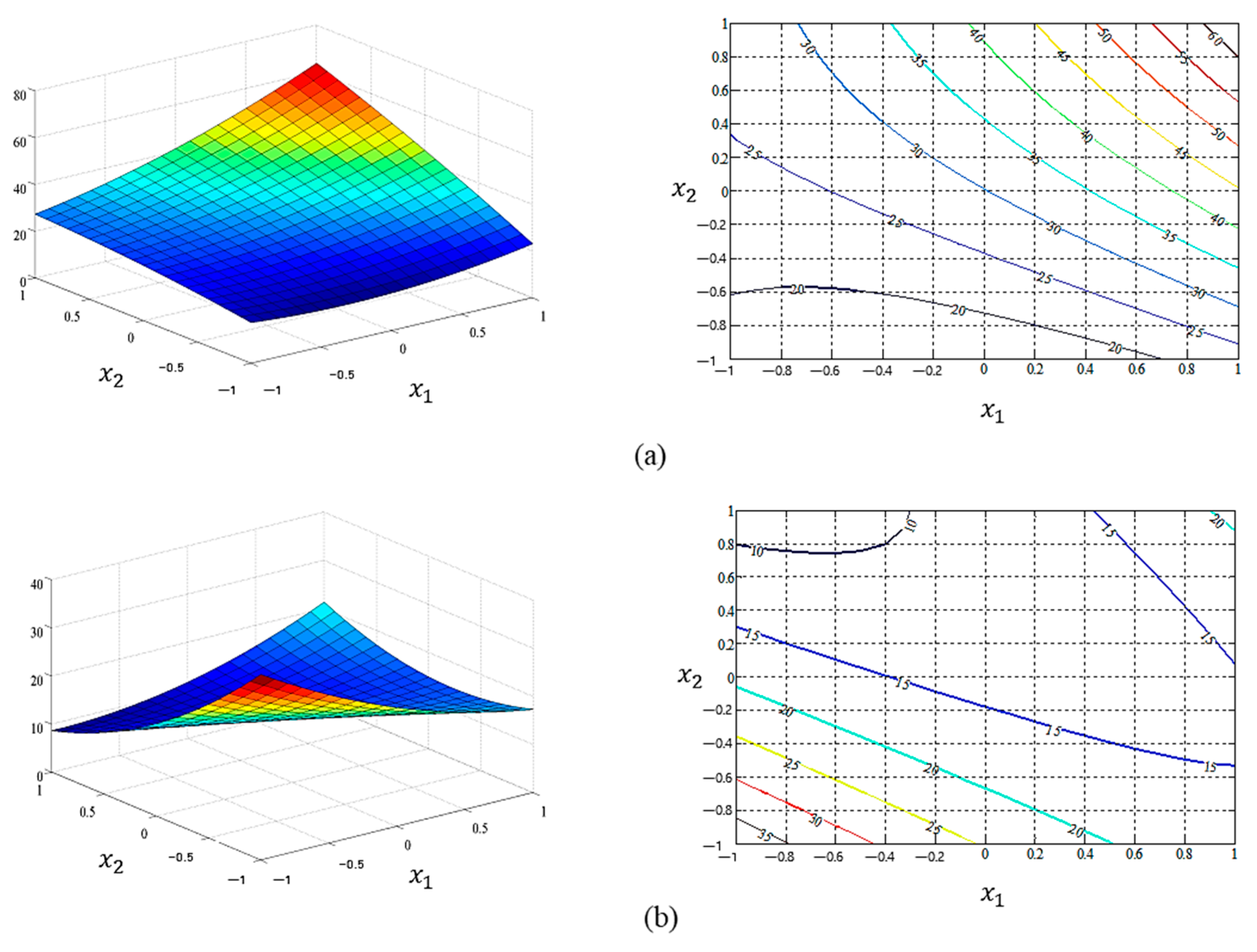
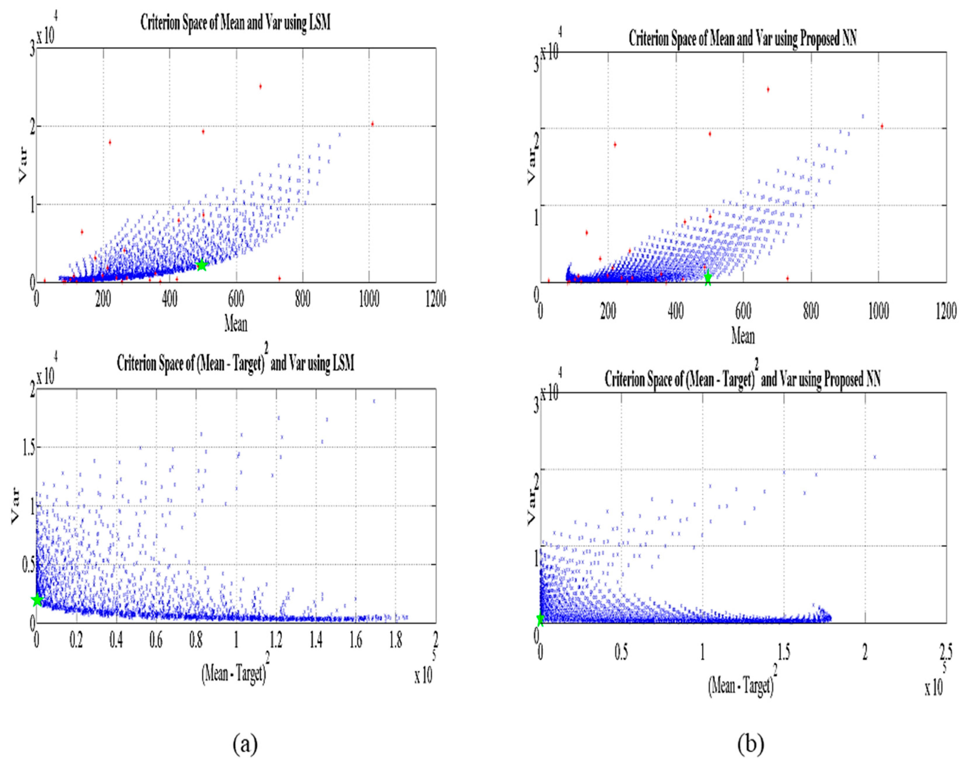
According to the estimated regression formulas of the process mean and standard deviation, the response functions of the dual-response models between parameters and for two estimation methods (i.e., LSM and NN) are illustrated in Figure 4 and Figure 5, including statistical indexes such as coefficients of determination and root-mean-square error (RMSE). The rest of parameters and , and are additionally provided as figures in Appendix A. The process mean, bias, and variance obtained from the proposed functional-link-NN-based dual-response estimation approach and the conventional LSM-based RSM are compared in Table 5 based on the corresponding optimal input variable settings and the EQL results. Table 5 implies that the proposed RD dual-response estimation approach based on the functional link NN produced a significantly smaller EQL value than the conventional LSM-based RSM. In addition, compared with the conventional LSM, the proposed method can provide lower process variance. The process mean and the squared bias with regard to the variability of the standard LSM-based RSM and proposed NN-based estimation model are shown in Figure 6. The criterion spaces of the estimated regression functions are denoted by red stars. The optimal settings are marked as green star in each figure.
5. Conclusions and Further Studies
There have been many studies to improve the RSM by combining statistical and mathematical techniques, but there are cases where particular data types are required or assumptions are made to define functions between mean, variance, and input elements. NNs, which have recently been widely applied in artificial intelligence, can present simple mathematical models (functions) using artificial neurons and determine unknown interactions between the input and output performance of a process without any knowledge of the principle.
This study has described a functional-link-NN-based estimation method that offers an alternative RD technique without assumptions inherent in the conventional LSM-based RSM. Compared with the existing RD dual-response estimation approach, the proposed method provides significant advantages in determining the functional relationship between the control factors and output performances and the optimal solutions. The proposed dual-response estimation approach can be quickly and efficiently implemented using MATLAB (see Appendix B). Experimental results show that the proposed NN-based estimation method can achieve better solutions than the conventional LSM-based RSM in the EQL metric.
In the future, the proposed functional-link-NN-based dual-response RD estimation approach will be extended to time series data and multiple-response optimization problems. In addition, we plan to search for the optimal structure by binary coding the neural network structure with a genetic algorithm and conducting research on optimizing the weights of the neural network.
Author Contributions
Conceptualization, T.-H.L. and S.S.; Methodology, T.-H.L. and S.S.; Modeling, T.-H.L.; Validation T.-H.L. and S.S.; Writing—Original Draft Preparation, T.-H.L. and S.S.; Writing—Review and Editing, M.T., J.H.J., H.J., and S.S.; Funding Acquisition, S.S. All authors have read and agreed to the published version of the manuscript.
Funding
This work was supported by the National Research Foundation of Korea (NRF) (No. NRF-2019R1F1A1060067).
Conflicts of Interest
The authors declare no conflict of interest.
Appendix A. The Estimated Regression Formulas of the Process Mean and Standard Deviation
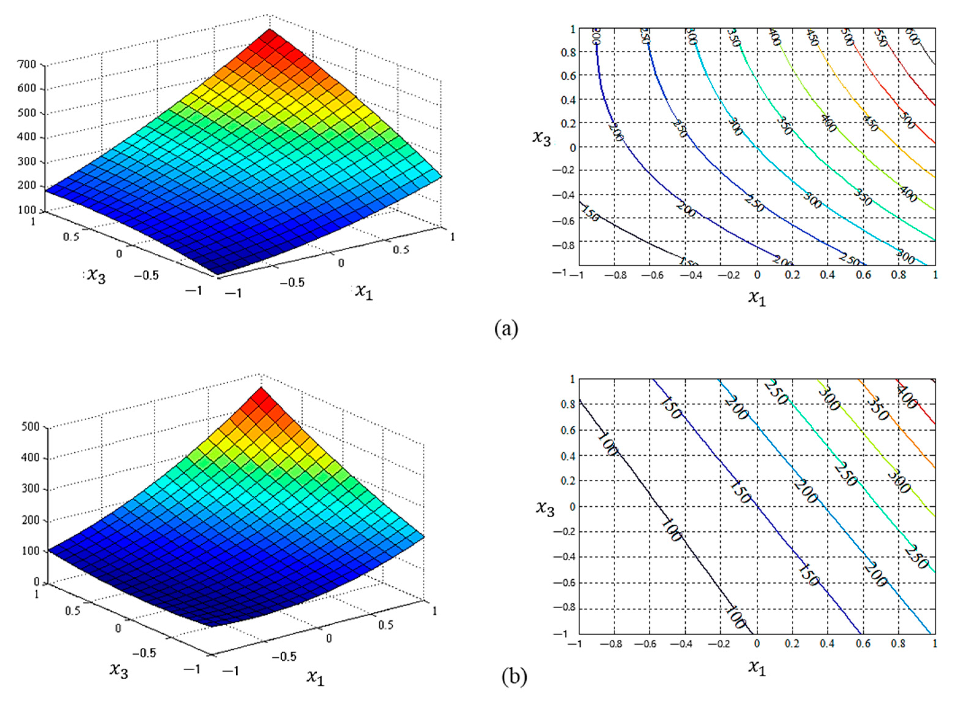
The estimated regression formulas of the process mean and standard deviation, the response functions of the dual-response model for the estimation methods, are illustrated in Figure A1, Figure A2, Figure A3 and Figure A4.
Figure A1.
Graphical representation of the estimated mean response functions between and : (a) the response surface plot and response function of LSM; (b) the response surface plot and response function of NN.
Figure A1.
Graphical representation of the estimated mean response functions between and : (a) the response surface plot and response function of LSM; (b) the response surface plot and response function of NN.

Figure A2.
Graphical representation of the estimated mean response functions between and : (a) the response surface plot and response function of LSM; (b) the response surface plot and response function of NN.
Figure A2.
Graphical representation of the estimated mean response functions between and : (a) the response surface plot and response function of LSM; (b) the response surface plot and response function of NN.

Figure A3.
Graphical representation of the estimated standard deviation response functions between and : (a) the response surface plot and response function of LSM; (b) the response surface plot and response function of NN.
Figure A3.
Graphical representation of the estimated standard deviation response functions between and : (a) the response surface plot and response function of LSM; (b) the response surface plot and response function of NN.

Figure A4.
Graphical representation of the estimated standard deviation response functions between and : (a) the response surface plot and response function of LSM; (b) the response surface plot and response function of NN.
Figure A4.
Graphical representation of the estimated standard deviation response functions between and : (a) the response surface plot and response function of LSM; (b) the response surface plot and response function of NN.

Appendix B. MATLAB Codes to Perform Estimative Regression Functions of Means and Standard Deviations by Using the Proposed NN Method

Table A1.
MATLAB codes of the proposed functional link NN method.
| MAIN FUNCTION %% Preparation %% data load dataprint.mat Target_mean = 500; y_mean = [dataprint(:,7)]; y_std = [dataprint(:,8)]; y_var = [dataprint(:,9)]; format long g %% prepare data X_NN = [dataprint(:,1:3)]’; y_mean_NN = y_mean’; y_std_NN = y_std’; y_var_NN = y_var’; samplesize_mean = size(y_mean_NN,2); sample_mean = size(y_mean_NN,1); samplesize_std = size(y_std_NN,2); sample_std = size(y_std_NN,1); [m,n] = size(X_NN); best1 = 1; best2 = 1; minBIC1 = 10e10; minBIC2 = 10e10; for i = 1:25 [net1, err1] = create_Poly2_mean(X_NN, y_mean_NN, i); mse1 = mse(err1); BIC1 = samplesize_mean*log(mse1/samplesize_mean) + m*log(samplesize_mean); if BIC1 <= minBIC1 minBIC1 = BIC1; best1 = i; end end Hidden_neuron_mean = best1; [net_mean_trained, err1] = create_Poly2_mean(X_NN, y_mean_NN, best1); mean_fun = @(x) sim(net_mean_trained, x); W_in_hid_mean = net_mean_trained.IW{1,1}; W_hid_out_mean = net_mean_trained.LW{2,1}; b_in_hid_mean = net_mean_trained.b{1,1}; b_hid_out_mean = net_mean_trained.b{2,1}; for j = 1:25 [net2, err2] = create_Poly2_std(X_NN, y_std_NN, j); mse2 = mse(err2); BIC2 = samplesize_std*log(mse2/samplesize_std) + m*log(samplesize_std); if BIC2 <= minBIC2 minBIC2 = BIC2; best2 = j; end end Hidden_neuron_std = best2; [net_std_trained, err2] = create_Poly2_std(X_NN, y_std_NN, best2); std_fun = @(x) sim(net_std_trained, x); W_in_hid_std = net_std_trained.IW{1,1}; W_hid_out_std = net_std_trained.LW{2,1}; b_in_hid_std = net_std_trained.b{1,1}; b_hid_out_std = net_std_trained.b{2,1}; %% NN_MSE: Optimal solutions options = optimset(‘Algorithm’,’interior-point’); objfun_NN = @(x) (mean_fun(x)-Target_mean)^2 + std_fun(x)^2; [x_opt_NN fval_opt_NN] = fmincon(objfun_NN, x0, [[], [[], [[], [[], lb, ub,[[],options); meanfun_opt_NN = mean_fun(x_opt_NN); stdfun_opt_NN = std_fun(x_opt_NN); results_MSE_NN = [x_opt_NN’ meanfun_opt_NN abs(meanfun_opt_NN-Target_mean) stdfun_opt_NN^2 fval_opt_NN] SUB-FUNCTION (TRAIN MEAN FUNCTION) |
| function [net,err] = create_Poly2_mean(inputs, targets, numHiddenNeurons) Number_Input = size(inputs,1); Number_Output = size(targets,1); net = Poly2_mean(Number_Input,Number_Output,numHiddenNeurons); %% Train and Apply Network net.trainFcn = ‘trainlm’; net.performFcn = ‘mse’; net.trainParam.epochs = 1000; net.trainParam.goal = 1e-5; net.trainParam.lr = 0.05;net.trainParam.show = 50; net.trainParam.showWindow = true; net.trainParam.max_fail = 100; net.divideFcn = ‘dividerand’; net = init(net); net.plotFcns = {‘plotperform’,’plottrainstate’,’plotregression’,’plotfit’}; [net,tr] = train(net,inputs,targets); bestEpoch = tr.best_epoch; trained = sim(net,inputs); err = targets-trained; end SUB-FUNCTION (TRAIN STANDARD DEVIATION FUNCTION) function [net,err] = create_Poly2_std(inputs, targets, numHiddenNeurons) Number_Input = size(inputs,1); Number_Output = size(targets,1); net = Poly2_std(Number_Input,Number_Output,numHiddenNeurons); %% Train and Apply Network net.trainFcn = ‘trainlm’; net.performFcn = ‘mse’; net.trainParam.epochs = 1000; net.trainParam.goal = 1e-5; net.trainParam.lr = 0.05; net.trainParam.show = 50; net.trainParam.showWindow = true; net.trainParam.max_fail = 100; net.divideFcn = ‘dividerand’; net = init(net); net.plotFcns = {‘plotperform’,’plottrainstate’,’plotregression’,’plotfit’}; [net,tr] = train(net,inputs,targets); bestEpoch = tr.best_epoch; trained = sim(net,inputs); err = targets-trained; end SUB-FUNCTION (CREATE MEAN FUNCTION) function net = Poly2_mean(Number_Input, Number_Output, numHiddenNeurons) net = network; %% Architect net.numInputs = 1; net.numLayers = 2; net.biasConnect(1) = 1; net.biasConnect(2) = 1; net.inputConnect(1,1) = 1; net.outputConnect = [0 1]; net.layerConnect = [0 0; 1 0]; %% layer1 net.inputs{1}.size = Number_Input; net.layers{1}.size = numHiddenNeurons; net.layers{1}.transferFcn = ‘Polyfunc2’; net.layers{1}.initFcn = ‘initnw’; %% layer2net.layers{2}.size = Number_Output; net.layers{2}.transferFcn = ‘purelin’; net.layers{2}.initFcn = ‘initnw’; %% net functionnet.initFcn = ‘initlay’; end SUB-FUNCTION (CREATE STANDARD DEVIATION FUNCTION) function net = Poly2_std(Number_Input, Number_Output, numHiddenNeurons) net = network; %% Architect net.numInputs = 1; net.numLayers = 2; net.biasConnect(1) = 1; net.biasConnect(2) = 1; net.inputConnect(1,1) = 1;net.outputConnect = [0 1]; net.layerConnect = [0 0; 1 0]; %% layer1 net.inputs{1}.size = Number_Input; net.layers{1}.size = numHiddenNeurons; net.layers{1}.transferFcn = ‘Polyfunc2_std’; net.layers{1}.initFcn = ‘initnw’; %% layer2 net.layers{2}.size = Number_Output; net.layers{2}.transferFcn = ‘purelin’; net.layers{2}.initFcn = ‘initnw’; %% net function net.initFcn = ‘initlay’; end SUB-FUNCTION (INTEGRATE FUNCTIONAL LINK TRANSFER FUNCTION INTO NN-BASED MEAN FUNCTION) function out1 = Polyfunc2(in1,in2,in3,in4) fn = mfilename; boiler_transfer %%%%%%%%%%%%%%%%%%%%%%%%%%%%%%%%%%%%%%%%% Name function n = name n = ‘Quadratic’; %%%%%%%%%%%%%%%%%%%%%%%%%%%%%%%%%%%%%%%%% Output range function r = output_range(fp) r = [-inf +inf]; %%%%%%%%%%%%%%%%%%%%%%%%%%%%%%%%%%%%%%%%% Active input range function r = active_input_range(fp) r = [-inf +inf]; %%%%%%%%%%%%%%%%%%%%%%%%%%%%%%%%%%%%%%%%% Parameter Defaults function fp = param_defaults(values) fp = struct; %%%%%%%%%%%%%%%%%%%%%%%%%%%%%%%%%%%%%%%%% Parameter Names function names = param_names names = {}; %%%%%%%%%%%%%%%%%%%%%%%%%%%%%%%%%%%%%%%%% Parameter Check function err = param_check(fp) err = ‘‘; %%%%%%%%%%%%%%%%%%%%%%%%%%%%%%%%%%%%%%%%% Apply Transfer Function function a = apply_transfer(n,fp) a = n.^2 + n; %%%%%%%%%%%%%%%%%%%%%%%%%%%%%%%%%%%%%%%%% Derivative of Y w/respect to X function da_dn = derivative(n,a,fp) da_dn = 2*n +1; SUB-FUNCTION (INTEGRATE FUNCTIONAL LINK TRANSFER FUNCTION INTO NN-BASED STANDARD DEVIATION FUNCTION) function out1 = Polyfunc2_std(in1,in2,in3,in4) fn = mfilename; boiler_transfer %%%%%%%%%%%%%%%%%%%%%%%%%%%%%%%%%%%%%%%%% Name function n = name n = ‘Quadratic polynomial Function’; %%%%%%%%%%%%%%%%%%%%%%%%%%%%%%%%%%%%%%%%% Output range function r = output_range(fp) r = [-inf +inf]; %%%%%%%%%%%%%%%%%%%%%%%%%%%%%%%%%%%%%%%%% Active input range function r = active_input_range(fp) r = [-inf +inf]; %%%%%%%%%%%%%%%%%%%%%%%%%%%%%%%%%%%%%%%%% Parameter Defaults function fp = param_defaults(values) fp = struct; %%%%%%%%%%%%%%%%%%%%%%%%%%%%%%%%%%%%%%%%% Parameter Names function names = param_names names = {}; %%%%%%%%%%%%%%%%%%%%%%%%%%%%%%%%%%%%%%%%% Parameter Checkfunction err = param_check(fp)err = ‘‘;%%%%%%%%%%%%%%%%%%%%%%%%%%%%%%%%%%%%%%%%% Apply Transfer Function function a = apply_transfer(n,fp) a = n + n.^2–11; %%%%%%%%%%%%%%%%%%%%%%%%%%%%%%%%%%%%%%%%% Derivative of Y w/respect to X function da_dn = derivative(n,a,fp) da_dn = 1 + 2*n; |
References
- Bendell, A.; Disney, J.; Pridmore, W.A. Taguchi Methods: Applications in World Industry; International Foundation for Science Publications: Bedford, UK, 1989; pp. 1–26. [Google Scholar]
- Dehnad, K. Quality Control, Robust Design and the Taguchi Method; Wadsworth and Brooks/Cole: Pacific Grove, CA, USA, 1989; pp. 243–254. [Google Scholar]
- Taguchi, G. Introduction to Quality Engineering: Designing Quality Into Products and Processes; Kraus International Publications: White Plains, NY, USA, 1986; pp. 153–176. [Google Scholar]
- León, R.V.; Shoemaker, A.C.; Kacker, R.N. Performance measures independent of adjustment: An explanation and extension of Taguchi’s signal-to-noise ratios. Technometrics 1987, 29, 253–265. [Google Scholar] [CrossRef]
- Box, G.E.P. Signal-to-noise ratios, performance criteria, and transformations. Technometrics 1988, 30, 1–17. [Google Scholar] [CrossRef]
- Box, G.; Bisgaard, S.; Fung, C. An explanation and critique of Taguchi’s contributions to quality engineering. Qual. Reliab. Eng. Int. 1988, 4, 123–131. [Google Scholar] [CrossRef]
- Nair, V.N.; Abraham, B.; MacKay, J.; Box, G.; Kacker, R.N.; Lorenzen, T.J.; Lucas, J.M.; Myers, R.H.; Vining, G.G.; Nelder, J.A.; et al. Taguchi’s parameter design: A panel discussion. Technometrics 1992, 34, 127–161. [Google Scholar] [CrossRef]
- Vining, G.G.; Myers, R.H. Combining Taguchi and response surface philosophies: A dual response approach. J. Qual. Technol. 1990, 22, 38–45. [Google Scholar] [CrossRef]
- Del Castillo, E.; Montgomery, D.C. A nonlinear programming solution to the dual response problem. J. Qual. Technol. 1993, 25, 199–204. [Google Scholar] [CrossRef]
- Copeland, K.A.F.; Nelson, P.R. Dual response optimization via direct function minimization. J. Qual. Technol. 1996, 28, 331–336. [Google Scholar] [CrossRef]
- Lin, D.K.J.; Tu, W. Dual response surface optimization. J. Qual. Technol. 1995, 27, 34–39. [Google Scholar] [CrossRef]
- Myers, R.H.; Montgomery, D.C. Response Surface Methodology: Process and Product Optimization Using Designed Experiments, 1st ed.; John Wiley & Sons: New York, NY, USA, 1995; pp. 1–12. [Google Scholar]
- Box-Steffensmeier, J.M.; Brady, H.E.; Collier, D. (Eds.) Oxford handbooks online. In The Oxford Handbook of Political Methodology; Oxford University Press: Oxford, UK, 2008. [Google Scholar]
- Lee, S.B.; Park, C.S. Development of robust design optimization using incomplete data. Comput. Ind. Eng. 2006, 50, 345–356. [Google Scholar] [CrossRef]
- Cho, B.R.; Choi, Y.; Shin, S. RETRACTED ARTICLE: Development of censored data-based robust design for pharmaceutical quality by design. Int. J. Adv. Manuf. Technol. 2010, 49, 839–851. [Google Scholar] [CrossRef]
- Cho, B.R.; Shin, S. Quality improvement and robust design methods to a pharmaceutical research and development. Math. Probl. Eng. 2012, 2012, 1–14. [Google Scholar] [CrossRef] [Green Version]
- Luner, J.J. Achieving continuous improvement with the dual approach: A demonstration of the Roman catapult. Qual. Eng. 1994, 6, 691–705. [Google Scholar] [CrossRef]
- Cho, B.R.; Park, C.S. Robust design modeling and optimization with unbalanced data. Comput. Ind. Eng. 2005, 48, 173–180. [Google Scholar] [CrossRef]
- Irie, B.; Miyake, S. Capabilities of three-layered perceptrons. In Proceedings of the IEEE International Conference on Neural Networks, San Diego, CA, USA, 24–27 July 1988; pp. 641–648. [Google Scholar]
- Hornik, K.; Stinchcombe, M.; White, H. Multilayer feedforward networks are universal approximators. Neural Netw. 1989, 2, 359–366. [Google Scholar] [CrossRef]
- Cybenko, G. Approximation by superpositions of a sigmoidal function. Math. Control Signal. Syst. 1989, 2, 303–314. [Google Scholar] [CrossRef]
- Funahashi, K. On the approximate realization of continuous mappings by neural networks. Neural Netw. 1989, 2, 183–192. [Google Scholar] [CrossRef]
- Rowlands, H.; Packianather, M.S.; Oztemel, E. Using artificial neural networks for experimental design in off-line quality. J. Syst. Eng. 1996, 6, 46–59. [Google Scholar]
- Shin, S.; Hoang, T.T.; Le, T.H.; Lee, M.Y. A new robust design method using neural network. J. Nanoelectron. Optoelectron. 2016, 11, 68–78. [Google Scholar] [CrossRef]
- Arungpadang, T.R.; Kim, Y.J. Robust parameter design based on back propagation neural network. Korean Manag. Sci. Rev. 2012, 29, 81–89. [Google Scholar] [CrossRef] [Green Version]
- Le, T.H.; Jang, H.; Shin, S. Determination of the Optimal Neural Network Transfer Function for Response Surface Methodology and Robust Design. Appl. Sci. 2021, 11, 6768. [Google Scholar] [CrossRef]
- Su, C.T.; Hsieh, K.L. Applying neural network approach to achieve robust design for dynamic quality characteristics. Int. J. Qual. Reliab. Manag. 1998, 15, 509–519. [Google Scholar] [CrossRef]
- Cook, D.F.; Ragsdale, C.T.; Major, R.L. Combining a neural network with a genetic algorithm for process parameter optimization. Eng. Appl. Artif. Intell. 2000, 13, 391–396. [Google Scholar] [CrossRef]
- Chow, T.T.; Zhang, G.Q.; Lin, Z.; Song, C.L. Global optimization of absorption chiller system by genetic algorithm and neural network. Energy Build. 2002, 34, 103–109. [Google Scholar] [CrossRef]
- Chang, H.H. Applications of neural networks and genetic algorithms to Taguchi’s robust design. Int. J. Electron. Bus. 2005, 3, 90–96. [Google Scholar]
- Chang, H.H.; Chen, Y.K. Neuro-genetic approach to optimize parameter design of dynamic multiresponse experiments. Appl. Soft Comput. 2011, 11, 436–442. [Google Scholar] [CrossRef]
- Arungpadang, T.A.R.; Tangkuman, S.; Patras, L.S. Dual Response Approach in Process Capability based on Hybrid Neural Network-Genetic Algorithms. JoSEPS 2019, 1, 117–122. [Google Scholar] [CrossRef] [Green Version]
- Villa-Murillo, A.; Carrión, A.; Sozzi, A. Forest-Genetic method to optimize parameter design of multiresponse experiment. Intel. Artif. 2020, 23, 9–25. [Google Scholar]
- Radosław, W.; Krzysztof, G.; Agnieszka, K.; Monika, J.M. Optimisation of ANN topology for predicting the rehydrated apple cubes colour change using RSM and GA. Neural Comput. Appl. 2018, 30, 1795–1809. [Google Scholar]
- Box, G.E.P.; Wilson, K.B. On the experimental attainment of optimum conditions [With discussion]. J. R. Stat. Soc. B 1951, 13, 1–38. [Google Scholar]
- Myers, R.H. Response surface methodology—Current status and future directions. J. Qual. Technol. 1999, 31, 30–44. [Google Scholar] [CrossRef]
- Khuri, A.I.; Mukhopadhyay, S. Response surface methodology. WIREs Comp. Stat. 2010, 2, 128–149. [Google Scholar] [CrossRef]
- Box, G.E.P.; Draper, N.R. Empirical Model—Building and Response Surfaces; John Wiley & Sons: New York, NY, USA, 1987; pp. 1–669. [Google Scholar]
- Khuri, A.I.; Cornell, J.A. Response Surface: Design and Analyses, 1st ed.; CRC Press: New York, NY, USA, 1987; pp. 1–536. [Google Scholar]
- Hartman, E.J.; Keeler, J.D.; Kowalski, J.M. Layered neural networks with Gaussian hidden units as universal approximations. Neural Comput. 1990, 2, 210–215. [Google Scholar] [CrossRef]
- Javadikia, P.; Rafiee, S.; Garavand, A.T.; Keyhani, A. Modeling of moisture content in tomato drying process by ANN-GA technique. In Proceedings of the 1st International Econference on Computer and Knowledge Engineering (ICCKE), Mashhad, Iran, 13–14 October 2011; IEEE Publications: Piscataway, NJ, USA, 2011; Volume 2011, pp. 162–165. [Google Scholar]
- Duch, W.; Jankowski, N. Transfer functions: Hidden possibilities for better neural networks. In Proceedings of the ESANN 2001, 9th European Symposium on Artificial Neural Networks, Bruges, Belgium, 25–27 April 2001; pp. 81–94. [Google Scholar]
- Sheela, K.G.; Deepa, S.N. Review on methods to fix number of hidden neurons in neural networks. Math. Probl. Eng. 2013, 2013. [Google Scholar] [CrossRef] [Green Version]
Figure 1.
Proposed feed-forward NN-based estimation procedure.

Figure 2.
Multilayer feed-forward NN structure.

Figure 3.
Functional-link-NN-based RD estimation method.

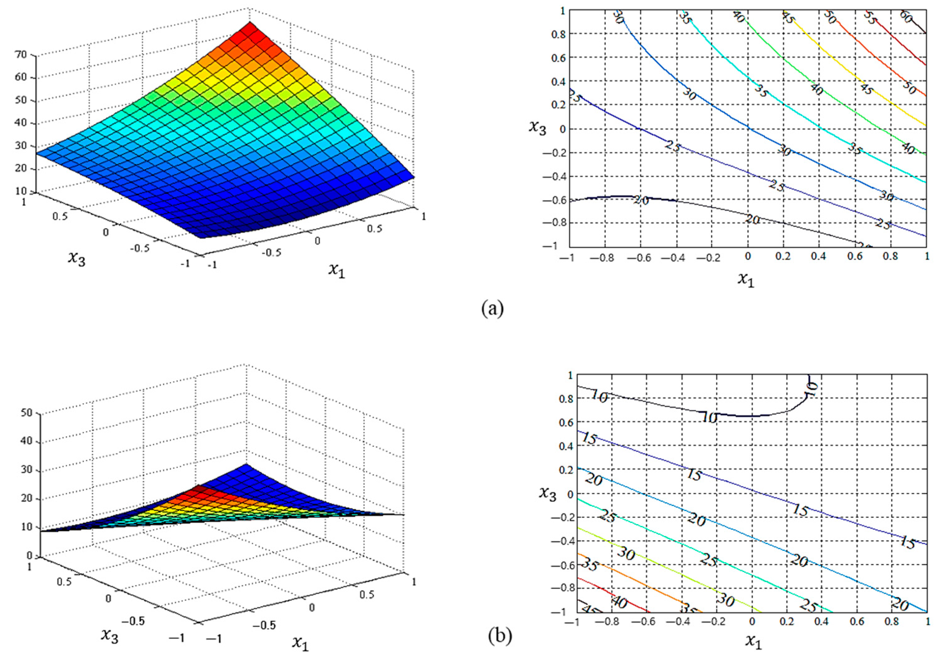
Figure 4.
Graphical representation of the estimated mean response functions between and : (a) the response surface plot and response function of LSM ( = 92.68% and RMSE = 60.40); (b) the response surface plot and response function of NN ( = 86.37% and RMSE = 82.47).
Figure 4.
Graphical representation of the estimated mean response functions between and : (a) the response surface plot and response function of LSM ( = 92.68% and RMSE = 60.40); (b) the response surface plot and response function of NN ( = 86.37% and RMSE = 82.47).

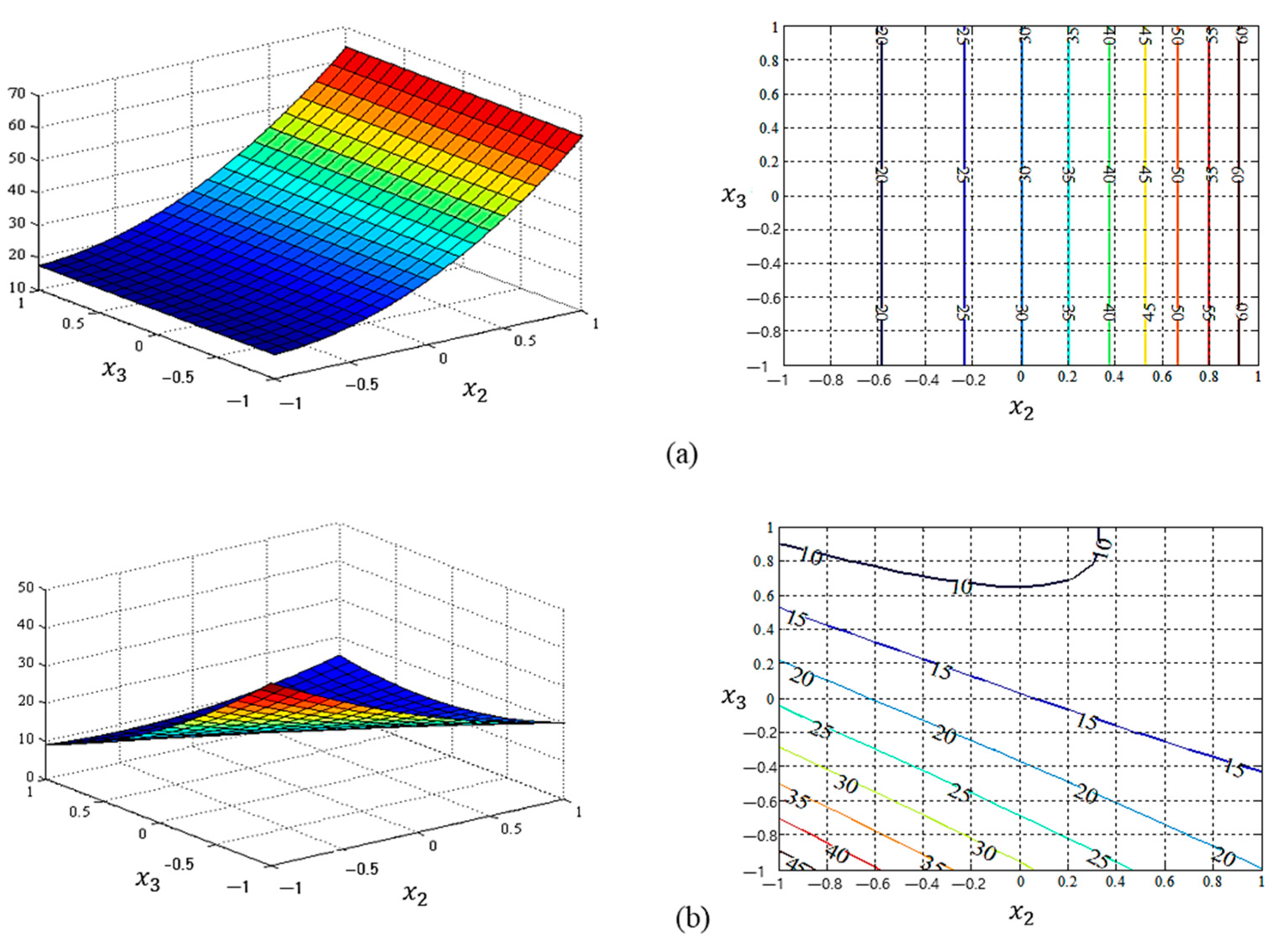
Figure 5.
Graphical representation of the estimated standard deviation response functions between and : (a) the response surface plot and response function of LSM ( = 45.41% and RMSE = 34.78); (b) the response surface plot and response function of NN ( = 44.18% and RMSE = 35.17).
Figure 5.
Graphical representation of the estimated standard deviation response functions between and : (a) the response surface plot and response function of LSM ( = 45.41% and RMSE = 34.78); (b) the response surface plot and response function of NN ( = 44.18% and RMSE = 35.17).

Figure 6.
Criterion space of the two estimated functions: (a) conventional LSM; (b) proposed NN-based RD estimation model.
Figure 6.
Criterion space of the two estimated functions: (a) conventional LSM; (b) proposed NN-based RD estimation model.

Table 1.
Coefficients of the estimated response functions using LSM.
| Treatment Combinations | Coefficients | |
|---|---|---|
| Constant | 327.630 | 34.883 |
| 177.000 | 11.527 | |
| 109.430 | 15.323 | |
| 131.460 | 29.190 | |
| 32.000 | 4.204 | |
| −22.389 | −1.316 | |
| −29.056 | 16.778 | |
| 66.028 | 7.720 | |
| 75.472 | 5.109 | |
| 43.583 | 14.082 | |
Table 2.
Parameters of NN-based estimation method.
| Objective | Response Function | Training Algorithm | Structure | No. of Epoch |
|---|---|---|---|---|
| Mean | mse | Trainlm | 3-21-1 | 13 |
| Std | mse | Trainlm | 3-2-1 | 12 |
Table 3.
Weight and bias terms of the NN for the estimated process mean.
| Weight | Bias | ||||
|---|---|---|---|---|---|
| 0.96075 | 0.11736 | 1.54028 | 2.10096 | 3.63174 | 1.00092 |
| 0.75123 | 0.38223 | 0.73934 | 1.62200 | 0.77913 | |
| −0.28537 | −0.34012 | −0.80124 | 2.30133 | 3.88614 | |
| 1.17461 | 0.63199 | 1.11264 | 1.73056 | 1.68918 | |
| 0.27560 | 0.60510 | −0.26521 | −0.48992 | −0.70557 | |
| −0.72625 | 0.41018 | 0.21240 | −0.11370 | −0.84332 | |
| −0.45138 | −0.37180 | 0.56006 | −1.03860 | −0.39605 | |
| −0.40578 | −0.11631 | −0.02559 | −0.09612 | −0.44870 | |
| 0.75884 | −0.59636 | −0.37276 | −0.29991 | −0.43415 | |
| 2.86524 | 1.95064 | 1.96605 | 4.72650 | 5.36510 | |
| −1.13144 | −0.73588 | −1.17218 | 0.84079 | −1.47882 | |
| −0.06226 | −0.41228 | −0.58818 | 0.40969 | 0.05234 | |
| 0.32760 | −0.75682 | −0.67588 | −0.11504 | −0.02238 | |
| −0.01851 | −0.81573 | 0.01320 | −0.27318 | −0.58988 | |
| 0.11633 | 0.16928 | 0.17376 | −0.45037 | −0.88337 | |
| −0.68532 | 0.37096 | −0.27889 | −0.27210 | 0.04470 | |
| −0.27500 | −0.52907 | 0.34659 | −0.85252 | −0.31859 | |
| 0.91857 | 0.59698 | 0.76126 | 0.59614 | 0.80572 | |
| 0.29861 | −0.39570 | 0.10545 | 0.28709 | 0.51167 | |
| 0.56297 | −0.03477 | −0.09037 | 0.43088 | 0.67887 | |
| 0.10126 | −0.37625 | −0.01066 | −0.64268 | −0.36799 | |
Table 4.
Weight and bias terms of the NN for the estimated process standard deviation.
| Weight | Bias | ||||
|---|---|---|---|---|---|
| −2.04505 | −3.02946 | −4.90330 | 0.86246 | −4.32652 | −0.01267 |
| −0.38368 | −1.22474 | −0.62419 | −2.32404 | −2.08030 | |
Table 5.
Comparative analysis results.
| Estimation Model | Optimal Factor Settings | Process Mean | Process Bias | Process Variance | EQL | ||
|---|---|---|---|---|---|---|---|
| LSM | 1.0000 | 0.07153 | −0.25028 | 494.67226 | 5.32773 | 1977.53266 | 2005.91742 |
| Proposed NN | 0.99999 | 0.99999 | −0.79327 | 496.39189 | 3.60810 | 450.64771 | 463.66611 |
Publisher’s Note: MDPI stays neutral with regard to jurisdictional claims in published maps and institutional affiliations. |
© 2021 by the authors. Licensee MDPI, Basel, Switzerland. This article is an open access article distributed under the terms and conditions of the Creative Commons Attribution (CC BY) license (https://creativecommons.org/licenses/by/4.0/).
Share and Cite
MDPI and ACS Style
Le, T.-H.; Tang, M.; Jang, J.H.; Jang, H.; Shin, S. Integration of Functional Link Neural Networks into a Parameter Estimation Methodology. Appl. Sci. 2021, 11, 9178. https://0-doi-org.brum.beds.ac.uk/10.3390/app11199178
AMA Style
Le T-H, Tang M, Jang JH, Jang H, Shin S. Integration of Functional Link Neural Networks into a Parameter Estimation Methodology. Applied Sciences. 2021; 11(19):9178. https://0-doi-org.brum.beds.ac.uk/10.3390/app11199178
Chicago/Turabian StyleLe, Tuan-Ho, Mengyuan Tang, Jun Hyuk Jang, Hyeonae Jang, and Sangmun Shin. 2021. "Integration of Functional Link Neural Networks into a Parameter Estimation Methodology" Applied Sciences 11, no. 19: 9178. https://0-doi-org.brum.beds.ac.uk/10.3390/app11199178
Note that from the first issue of 2016, this journal uses article numbers instead of page numbers. See further details here.