Phishing Webpage Classification via Deep Learning-Based Algorithms: An Empirical Study

Abstract

Phishing detection with high-performance accuracy and low computational complexity has always been a topic of great interest. New technologies have been developed to improve the phishing detection rate and reduce computational constraints in recent years. However, one solution is insufficient to address all problems caused by attackers in cyberspace. Therefore, the primary objective of this paper is to analyze the performance of various deep learning algorithms in detecting phishing activities. This analysis will help organizations or individuals select and adopt the proper solution according to their technological needs and specific applications’ requirements to fight against phishing attacks. In this regard, an empirical study was conducted using four different deep learning algorithms, including deep neural network (DNN), convolutional neural network (CNN), Long Short-Term Memory (LSTM), and gated recurrent unit (GRU). To analyze the behaviors of these deep learning architectures, extensive experiments were carried out to examine the impact of parameter tuning on the performance accuracy of the deep learning models. In addition, various performance metrics were measured to evaluate the effectiveness and feasibility of DL models in detecting phishing activities. The results obtained from the experiments showed that no single DL algorithm achieved the best measures across all performance metrics. The empirical findings from this paper also manifest several issues and suggest future research directions related to deep learning in the phishing detection domain.

1. Introduction

In the past few years, deep learning (DL) techniques have proven to be an effective solution among applications across multiple disciplines, including Internet of Things (IoT), intrusion detection system (IDS), ransomware detection, etc. [1,2,3,4,5]. Numerous researchers in cyber security have shifted their attention towards DL algorithms. Notably, researchers and security experts have also recognized its significance in the phishing detection domain [6,7,8]. During the last few years, website phishing has become one of the most common phishing attacks in cyberspace. Therefore, various anti-phishing solutions have been developed to detect phishing threats early to minimize the security risks and protect the end-users. Among them, website phishing detection based on DL algorithms has caught much attention in recent studies. Security strategies based on DL mechanisms have become increasingly popular to deal with evolving phishing attacks [9,10,11]. There are numerous types of DL techniques designed to solve a specific problem or meet a system’s particular requirement; each has its advantages and disadvantages [2,12,13].

Hence, choosing the right approach best fitted to a target application is not an easy task. Especially when phishers keep changing their attacking tactics to leverage the systems’ vulnerabilities and the users’ unawareness, selecting an inappropriate algorithm would lead to unpredicted outcomes, resulting in a waste of effort and eventually affecting the model’s accuracy and efficiency [14]. Therefore, choosing an effective phishing detection model, high in performance accuracy and low in computational power, is a challenging task. The fine-tuning process of DL architectures is another issue that needs to be considered. Motivated to solve this problem, this paper adopted an empirical approach to explore the performance of several DL algorithms, such as deep neural network (DNN), convolutional neural network (CNN), Long Short-Term Memory (LSTM), and gated recurrent unit (GRU). This paper also identified the parameter settings for each DL model and investigated the effects of changing these parameters on the model’s performance accuracy. The final goal of this paper was to choose the best DL algorithm with the neural network architecture that produced the maximum accuracy with the minimum computational consumption. The findings from the empirical analysis of this paper also highlight the overlooked issues and future perspectives that encourage researchers to solve these problems.

This paper continues our previous research work that described a systematic literature review on phishing detection and machine learning [15]. One of the findings from this work suggested that DL algorithms appeared to be an effective solution for detecting phishing attacks, yet they have not been fully exploited. In this regard, an empirical analysis was conducted in this study to explore the most recent DL techniques used for phishing detection. In this paper, the following contributions were made via the empirical study:

• We exploited the state-of-the-art DL algorithms and compared their performance using numerous evaluation metrics;
• We identified the most common parameters and examined their influences on the performance of four DL models;
• We highlighted several issues based on the findings from the empirical experiments and recommended possible solutions to address these issues.

The remainder of this paper is structured as follows. Section 2 provides a short description of four different DL architectures, and reviews previous studies on these algorithms in the phishing detection domain. The methodology used to conduct this research is presented in Section 3, including experiment setup, website features, DL models, and parameter optimization. Section 4 summarizes the findings, highlights the issues observed from the obtained results, and suggests possible solutions for future research directions. Finally, the conclusion and future work of this research is given in Section 5.

2. Literature Review

This section provides a general overview of four different DL algorithms, including DNN, CNN, LSTM, and GRU. Previous research on these four types of DL architectures in the phishing detection domain is also discussed. In each study, we analyzed the neural network architecture, parameter optimization, and performance metrics to achieve a comprehensive understanding of each DL model’s design, implementation, and evaluation. Finally, the novelty of this research work compared with other related studies in the same research area is also highlighted.

2.1. Deep Neural Network (DNN)

Deep neural network (DNN) is one of the most common types of DL algorithm widely used in the cybersecurity domain. DNN is well-known among DL architectures due to its success in a wide range of applications [13], its ability to express complex functions with fewer parameters, and its capability to facilitate feature extraction and representation learning [16]. However, DNN requires a substantial amount of labeled data for training. In addition, it still suffers from insufficient parameter selection techniques [17], and the learning process is time-consuming [13]. Despite its disadvantages, several research works have been conducted to examine the effectiveness of applying DNN in detecting phishing webpages.

Table A1. Previous research works on DNN.

Reference	Dataset	Dataset Size	Number of Neurons			Learning Rate	Batch Size	Epoch
			Input	Hidden	Output
[18]	UCI	11,055	30	20/10/5	2	0.01	-	<200
[19]	PhishTank	73,575	-	20/40	-	-	-	100
	Yandex
[22]	UCI	17,700	-	-	-	-	-	-
	DMO	10,000
[42]	PhishTank	2119	10	19/100/200/300	1	0.0001	-	6000
	Alexa	1407
[21]	PhishTank	17,000	-	-	-	-	-	-
	DMOZ	20,000
	PageRank	480
	WHOIS	480
[64]	PhishTank Yahoo Own dataset	11,055	30	20/10/5	2	0.001	32	150
		1353	9	-	2
		58,645	111	-	2
		88,657	111	-	2
[20]	PhishTank Alexa	3000	10	20/100/200/300/400/500	1	0.001		3100

in Appendix A summarizes previous studies related to DNN for phishing detection, in the literature.

As a single classifier, DNN was used in [18,19,20] to train the classification system for the detection of phishing websites. Instead of using DNN as a stand-alone classifier, the authors in [21,22] combined it with other DL algorithms to build a model to differentiate between malicious and benign URLs. It was observed that among these DNN-based models, parameters settings play an essential role in determining the system’s performance accuracy. Nevertheless, some studies [21,22] did not mention any of the hyper-parameters in the design of the neural network architecture, while other papers [19,20] only specified a few of them without performing parameter optimization. The authors in [18] made additional effort in fine-tuning the parameters, but not all were included.

Moreover, the performance metric is another crucial factor that needs to be considered when analyzing and evaluating a phishing detection system. Previous studies have shown a limited number of metrics were used to assess the performance of DL models in detecting phishing websites. For example, only two metrics were used in [19], and three were measured in [21]. More metrics were used in the studies [18,22], yet only the selected ones were utilized to benchmark with other machine learning classifiers.

2.2. Convolutional Neural Network (CNN)

Convolutional Neural Network (CNN) is another popular type of DL technique in the field of cybersecurity. CNN is well-fitted to multi-dimensional data and specializes in image and signal processing [1,23]. In addition, CNN can extract features from raw data more efficiently and can solve complicated tasks. It is also more scalable and requires less training time [4]. Nevertheless, CNN architecture needs high computational power and a big dataset when dealing with image data [13]. Although CNN has achieved tremendous success with computer vision, it has also been applied in the cybersecurity domain.

Table A2. Previous research works on CNN.

Reference	Dataset	Dataset Size	Number of Kernels	Kernel Size	Pooling Size	Stride	Learning rate	Dropout Rate	Batch Size	Epoch
[37]	NA	2000	-	5	-	-	-	-	16	-
[7]	PhishTank	318,642	256	3	3	-	-	0.5	128	20
	Com Crawl	73,575
	Yandex	83,857
	Alexa	82,888
[8]	PhishTank	2456	64 32	16 16	-	-	-	-	-	-
	Millersmiles
	Yahoo
	Starting point
[10]	PhishTank	21,303	-	128	3	1	0.001	0.5	64	10
	Alexa/Amazon	24,800
[11]	PhishTank	4,820,940	32	3 × 1	2	3 × 1	0.0001	0.5	-	-
	Openphish		16
	Alexa		8
[25]	DMOZ Own dataset	3816	32	3 × 3	(2,2)	-	-	-	32	61
			32
			64
[26]	ILSVRC-2012-CLS	12	-	-	-	-	0.01	-	32	5000
[30]	PhishTank	2,585,146	64	2	-	-	-	0.2	64	3
			64	3				0.5
[42]	PhishTank	2119	32/64/64/128/128/264/512	-	2	1	0.001	-	-	200
	Alexa	1407
[31]	Alexa, DMOZ, etc., Sophos	611,894124,574	64	5	4	-	0.001	-	-	500
[29]	PhishTank	13,652	8/16/32/64/84	1/3/5/7/9	-	-	-	-	-	-
	Crawler	10,000
[24]	PhishTank	10,604	-	2	2	2	0.1 0.01 0.001 0.0005	0.5	45	15
	Common Crawl	10,604
[32]	PhishTank	245,385	-	5/6/7	-	-	0.01	0.9	2048	32
	Alexa	245,023
[27]	PhishTank	43,984	-	5	-	-	-	-	10	50
	5000 Best Websites	45,000
[33]	PhishTank	1,021,758	-	-	-	-	-	-	64	20/45/64
	DMOZ	989,021
[35]	PhishTank	97,400	256	5/6/7	4	-	0.0001	-	32	200
	Virus Total
	Yandex	97,400
[28]	UCI	11,055	8/16/32/64	10	2	-	-	-	-	220
				5
[34]	Own dataset	340,000	128	2	-	-	0.01	0.5	100	30
		65,000	128	4
[38]	PhishTank	206,200	200	2	2	1	-	-	-	-
	MalwarePatrol
	DMOZ, Alexa

from Appendix A provides a summary of previous research works on CNN in the field of phishing detection.

CNN was used as a single classifier in numerous research to distinguish between phishing and legitimate websites [7,8,20,24,25,26,27,28]. It can also be used in combination with other DL techniques to form an ensemble model and to improve phishing detection accuracy [10,11,29,30,31,32,33,34,35,36]. The difference between the architectures of CNN and DNN is the use of convolutional layers and kernels. Realizing the important role of these elements in determining the performance accuracy of phishing detection models, most researchers paid more attention to specifying these parameters, not others such as learning rate, dropout rate, epoch, or batch size. While this problem was avoided in [10], details of optimizing these parameters were not provided in the paper. Similarly, the authors of [24,28,29,32] described the optimization process, but only on certain parameters, for example, the number of convolutional layers, number of kernels, and kernel size. Additionally, in terms of performance metrics, it was observed that accuracy, precision, recall, and F1-score were the most common measures [7,24,28,30,31,32,34,35,37,38]. Other evaluation metrics were training time, detection time, GPU memory requirement, etc. [7,24,28,32,33,34].

2.3. Long Short-Term Memory (LSTM)

Long Short-Term Memory (LSTM) is a type of Recurrent Neural Network (RNN) that involves a loop structure between neurons in each layer [12]. LSTM is suitable for sequential or time-series data since it can maintain the continuity of information [39]. LSTM is more popular than the original RNN because the vanishing or exploding gradient and long-term dependency problems in traditional RNN have been overcome in LSTM [1,3,4]. LSTM takes a significantly long time to train, despite these advantages, compared to other DL algorithms [1]. In addition, LSTM only considers the forward information and does not consider the backward information. This issue, however, can be resolved in Bidirectional LSTM [40]. LSTM has caught much attention among researchers, and some of their research works in the phishing detection domain are shown in

Table A3. Previous research works on LSTM.

Reference	Dataset	Dataset Size	Number of Layers	Number of Units	Learning Rate	Dropout Rate	Batch Size	Epoch
[41]	PhishTank	1.5 million	1	128	0.0001	-	-	25
	Common Crawl		2
[46]	PhishTank	153,788	1	100	0.001	0.2	64	30
	Openphish	7212
	Alexa	170,552
[42]	PhishTank	2119	-	4	0.001	-	-	700
	Alexa	1407
[31]	Alexa, DMOZ, etc., Sophos	611,894 124,574	1	70	0.001	-	-	500
[44]	Vaderetro	2000	1	-	-	-	-	200
	Alexa	1,000,000
[43]	PhishTank	2000	5	128	0.001	-	128	-
	Yahoo Directory	2000
[33]	PhishTank	1,021,758	-	-	-	-	64	20/140/ 256/578
	DMOZ	989,021
[35]	PhishTank	97,400	1	32	0.0001	-	32	200
	Virus Total
	Yandex	97,400
[10]	PhishTank	21,303	1	128	0.001	0.5	64	10
	Alexa/Amazon	24,800
[11]	PhishTank	4,820,940	2	128	0.0001	0.5	-	-
	Openphish
	Alexa
[47]	UCI	2456	1	-	0.001	-	-	200
			2		0.0001			600
			3		0.0001			800
			4		0.01			900
			5		0.0001			1000
[45]	PhishTank	450,176	1	10	-	0.2	-	10
[36]	OpenPhish Alexa	52,000	-	-	-	-	-	-

(Appendix A).

Similar to DNN and CNN, LSTM can be implemented individually [20,41,42,43,44,45], incorporated with traditional machine learning techniques [46,47], or combined with other DL algorithms in a hybrid model for an improved performance in detecting malicious websites [10,11,31,33,35,36]. Among the studies of LSTM-based phishing detection models, a majority of them specified the parameter settings for neural network architecture, number of epochs, and learning rate; but ignored the dropout rate and batch size [31,41,42,44,47]. Moreover, only certain parameters were optimized during the fine-tuning process [32,42]. To evaluate the overall performance of LSTM models, four popular metrics were used, being accuracy, precision, recall, and F1-score [31,35,41,44,45]. Other measures training time, detection time, error rate, detection cost, number of epochs per second, etc. [33,42,46,47].

2.4. Gated Recurrent Unit (GRU)

Gated Recurrent Unit (GRU) is another variant of RNN and is a lightweight version of LSTM [23]. While working on small datasets, the performance of GRU is similar to LSTM [48]. Some of the previous studies that implemented GRU in their phishing detection models are provided in

Table A4. Previous research works on GRU.

Reference	Dataset	Dataset Size	Number of Layers	Number of Units	Learning Rate	Dropout Rate	Batch Size	Epoch
[41]	PhishTank Common Crawl	1.5 million	1 2	128	0.0001	-	-	25
[34]	Own dataset	340,000 65,000	1	64	0.01	0.5	100	30
[48]	PhishTank Common Crawl	759,361	2	60	0.001	-	256	20

(Appendix A).

There are a limited number of studies on the implementation of GRU for phishing detection. GRU and Bidirectional GRU can be employed as a single classifier [41,48], or as a replacement to the max-pooling layer in a CNN model [34]. Similar to LSTM, in implementing GRU-based phishing detection models, only neural network architecture, learning rate, and epoch were specified, but not batch size and dropout rate [41,48]. Plus, none of the reviewed papers on GRU included parameter optimization in their experiments. Regarding the performance metrics, all three studies [34,41,48] used accuracy, precision, recall, and F1-score to assess the effectiveness of the DL algorithm. Additional metrics involved GPU memory requirement and parameter set size [34,48].

2.5. Hyper-Parameters

One of the factors that affects the performance of DL algorithms is the selection of hyper-parameters during training. Their values can be fine-tuned to optimize the performance accuracy of phishing detection models. These parameters include, but are not limited to, the number of layers in the neural networks, number of neurons (units) in each layer, learning rate, dropout rate, number of epochs, batch size, etc. [17]. A basic understanding of each parameter will assist in selecting its value in the design and implementation of various DL architectures.

Learning rate. Learning rate is one of the essential factors in the parameter settings of DL models to determine how proper the network can be trained or how fast the model can converge [22,42]. As the learning rate is associated with the convergence speed of the DL algorithm, a more significant learning rate (0.5 to 1) results in a faster convergence speed [49]. A higher learning rate guarantees not only good performance but also causes low stability. However, this only happens at the early stage; after a certain period, the model’s performance will slow down and eventually stop before reaching optimality. Meanwhile, a smaller learning rate (0.0001 to 0.01) can guarantee the model’s stability, yet it delays the speed of convergence, and hence, a longer time is needed to train the DL algorithm.

Dropout rate. Dropout is one of the regularization techniques used to avoid overfitting problems in deep neural network architectures [23]. Overfitting usually happens when the DL model performs well on the training dataset but does not perform well on the validation set. This causes the training accuracy to be much higher than the validation accuracy. The dropout rate is a probability coefficient at which neurons in a particular layer of deep neural networks are discarded during the training process [33]. For instance, when a dropout rate of 0.2 is applied to a specific layer, 20% of the total number of neurons in that particular layer will be dropped. Dropout strategy is usually used in CNN, LSTM, and GRU architectures to prevent overfitting issues [10,30,34].

Batch size. In implementing a DL algorithm, a dataset consisting of numerous samples is used and split into two parts, namely training and testing. In the training phase, instead of passing the whole set of samples to the DL model, training data is divided into batches, in which each batch contains a small amount of data. The size of this subset of data is known as batch size [50]. The normal range of batch size is from 16 [37] to 2048 [32], depending on the size of the dataset. Small datasets generally use small batch sizes, while big datasets use larger batch sizes.

Epoch. Epoch is the number of iterations for training after the DL model has been built and compiled. It is essential to select the appropriate number of training iterations since it can affect the performance accuracy of the phishing detection model [22]. The detection accuracy can increase as the number of epochs goes higher; however, it also requires longer training of the deep neural network. As a result, to determine the number of epochs that give the best performance, one can increase the number of training iterations until reaching the minimum loss. With the growing number of epochs, the model loss will continue to decrease to a specific minimum value and then fluctuate [42]. At this point, training should be stopped since the model accuracy remains stagnant for a further higher number of iterations.

Number of layers. Network layers refer to the hidden layers in DNN, the convolutional layers in CNN, the LSTM/GRU layers in LSTM/GRU architecture, the Restricted Boltzmann Machine (RBM) layers in Deep Belief Network (DBN), the number of Autoencoders (AE) in the Stacked Autoencoder (SAE) model, etc. [22]. An increase in the number of layers in neural network architecture will increase network complexity and slow down the training process. Consequently, it is advisable to slowly raise the number of layers while observing the model’s performance accuracy. Further increase in layers might result in additional processing time while the best performance cannot be guaranteed [42].

Number of neurons/units per layers. In addition to network layers, the number of neurons or units in each layer can also significantly impact the performance of the DL algorithm. Similarly, increasing the number of neurons in the hidden layers of the Deep Neural Network or the number of LSTM units in the LSTM layers might cause low detection accuracy and long training time [42]. Therefore, researchers need to fine-tune these values to ensure an effective and efficient DL model for phishing detection without compromising its performance accuracy.

Number of kernels. Instead of the number of neurons in the hidden layers of DNN, in CNN architecture, the number of kernels or filters in the convolutional layers can significantly influence the success rate at which phishing websites are detected. Kernels, or filters, are used mainly in CNN models to convolve the input data into numerous feature maps [22]. Different kernels were used in previous research works, ranging from 8 [11] to 512 [42], depending on the number of input features, size of the dataset, or the neural network architecture.

Kernel size. Kernel size, or window size, is another parameter that needs to be fine-tuned in CNN models. Kernel size is the size of a one-dimensional window, which is convolved sequentially in the convolutional layers and depends on the number of input features [42]. Different kernel sizes have been utilized in previous studies, with typical values from 1 to 10 [28,29,35]. The optimal kernel size that produces the best performance is determined based on the model’s loss and accuracy.

Optimizer. While training deep neural networks, the loss function or error is calculated to evaluate the effectiveness and efficiency of the DL algorithm. This loss function can be optimized, and the weights can be updated by using optimizers [34,42]. Popular methods of optimization include Root Mean Square Propagation (RMSProp), Gradient Decent (GD), Adam, AdaGrad, AdaDelta, etc. [26]. GD and Adam are the most common optimization techniques in classification problems to optimize the error and adjust the weights [37].

Activation function. The activation function is represented by a mathematical equation that defines an output of a neuron based on given inputs [13]. It is considered one of the important parameters in DL architectures that determines the training model’s output, accuracy, and efficiency. In the neural network, neurons of the same layer usually use the same activation function [6]. Rectified Linear Unit (ReLU), Softmax, sigmoid, and Tanh are examples of frequently-used activation functions for DL models.

2.6. Performance Metrics

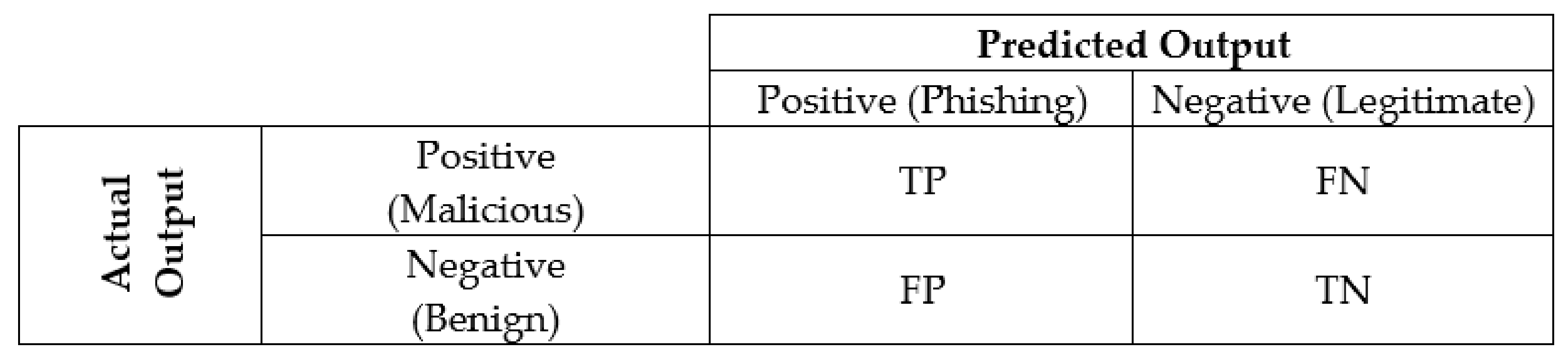
To evaluate the performance of a typical DL model, several metrics can be used. The most common is the confusion matrix which comprises four basic measures: True Positive (TP), True Negative (TN), False Positive (FP), and False Negative (FN), as shown in Figure 1. In addition, Precision, Recall, F1-Score, Area Under the Curve, and Accuracy are also important metrics that are required in the performance evaluation of phishing detection models. The formula of these metrics can be defined as Equations (1)–(6). In any phishing detection model, the primary purpose is to identify phishing attacks; therefore, a phishing sample is often regarded as a positive instance while a legitimate sample is considered as a negative instance [3,41,51].

• True Positive (TP) is the number of positive instances that the model has correctly classified or the number of samples that have accurately been labeled as phishing [2,52,53].
• True Negative (TN) represents the number of negative instances that the model has correctly predicted or the number of samples that have accurately been categorized as legitimate [2,52,53].
• False Positive (FP) denotes the number of negative instances that have been incorrectly recognized as positive or the number of legitimate samples that have been misclassified as phishing [2,52,53].
• False Negative (FN) refers to the number of positive instances that have been wrongly labeled as negative, or the number of malicious samples that have been misidentified as benign [2,52,53].

False Positive Rate (FPR), also known as False Alarm Rate (FAR) or Fall-Out, is defined as the ratio of FP instances to the total number of predicted negative samples. In other words, it is the number of legitimate instances incorrectly classified as phishing over the total number of legitimate samples [2,46], and is measured as follows:

$$\mathrm{FPR}=\frac{\mathrm{FP}}{\mathrm{FP}+\mathrm{TN}}$$

(1)

False Negative Rate (FNR) is defined as the ratio of FN instances to the total number of predicted positive samples, or the percentage of phishing instances wrongly marked as legitimate in all the phishing samples [2,46], and is calculated as:

$$\mathrm{FNR}=\frac{\mathrm{FN}}{\mathrm{FN}+\mathrm{TP}}$$

(2)

Precision (PR) is the fraction of predicted positive instances that are positive [1], or the proportion of phishing samples correctly classified as phishing over the total number of actual phishing samples [46,52]. PR indicates the confidence level of the phishing detection model, i.e., how many are malicious out of all the phishing instances detected [18]. PR can be used as a valuable measure for situations in which an unbalanced dataset is involved, in cases when accuracy fails to indicate how well the DL model performs, or in scenarios where the accuracy score alone is insufficient for security experts to make a decision [1]. High precision indicates how accurately the model can detect phishing attacks. PR can be computed using the following formula:

$$\mathrm{PR}=\frac{\mathrm{TP}}{\mathrm{TP}+\mathrm{FP}}$$

(3)

Recall (RC), also known as True Positive Rate (TPR), Sensitivity, or Probability of Detection (P_D) [54], represents the percentage of positive instances in all predicted positive samples. It shows the proportion of phishing instances accurately recognized as phishing over the total number of predicted phishing samples [46]. RC can sometimes be named as detection rate [3], which reflects the model’s ability to identify phishing activities, and is mathematically given by:

$$\mathrm{RC}=\frac{\mathrm{TP}}{\mathrm{TP}+\mathrm{FN}}$$

(4)

F1-Score (F1), or F-Measure, is a harmonic means of precision and recall, representing the balance of both these measurements. F1-Score is a good indication of how well the model has performed [1]. A high F1 value means the model can detect malicious attacks while ensuring that FP and FN are minimized. F-Measure signifies the model’s resilience and effectiveness [32,55]. Thus, it can be used to estimate the overall performance of the DL model and is given by the following equation:

$$\mathrm{F}1=2.\frac{\mathrm{PR}.\mathrm{RC}}{\mathrm{PR}+\mathrm{RC}}$$

(5)

Area Under the Curve (AUC) is measured as the total area under a Receiver Operating Characteristic (ROC) curve, which is a graph plotted with the FPR as x-axis and TPR as y-axis [54]. It describes the model’s classification ability while varying the classification thresholds and typically ranges between 0.5 and 1.0 [51]. AUC closed to 1.0 is an ideal scenario with perfect classification capability, whereas AUC less than 0.5 indicates an inferior detection performance. In other words, the higher the AUC value, the better the classifier.

Accuracy (ACC) is one of the most essential and popular metrics to assess the performance of a DL algorithm [1]. In the context of phishing detection, it shows how effectively and efficiently a classifier can distinguish between phishing and legitimate. ACC measure can be used as a good indicator of how well a DL model is trained and described as the overall effectiveness of the classification model [2]. There are certain limitations with accuracy when it comes to unbalanced datasets. However, valuable insight can be derived from accuracy measures when the classes are balanced [54]. ACC is calculated as the ratio of correctly classified instances (both phishing and legitimate) to the total input samples (the whole dataset). The equation used for the measurement of accuracy is as follows:

$$\mathrm{ACC}=\frac{\mathrm{TP}+\mathrm{TN}}{\mathrm{TP}+\mathrm{TN}+\mathrm{FP}+\mathrm{FN}}$$

(6)

2.7. Research Novelty

This section highlights the novelty of this empirical study, which is viewed from three perspectives: specification of parameter settings in neural network architectures, optimization process of hyper-parameters for DL algorithms, and performance metrics for phishing detection model evaluation.

Even though DL offers various advantages, one of its major drawbacks is manual parameter tuning. There is no standard and holistic guideline for selecting these hyper-parameters to achieve the highest performance accuracy.

Table 1. Frequency of parameter settings for DL architectures.

Category	Algorithm	Frequency				Reference
		NS 1	RS 2	PS 3	FS 4
Single	DNN	-	1	-	-	[19]
	MLP	1	-	2	-	[6,56,57]
	CNN	-	-	4	-	[7,8,25,27]
	LSTM	-	1	1	-	[44,45]
	BiLSTM	1	-	-	-	[58]
	BiGRU	-	-	1	-	[48]
Dual	CNN, CNN	-	-	1	-	[37]
	CNN, LSTM	1	-	4	-	[30,31,33,59,60]
	CNN, BiLSTM	3	-	1	-	[10,36,40,61]
	CNN, GRU	-	-	1	-	[34]
Multiple	CNN, RNN, MLP	-	-	1	-	[11]
	DNN, DBM, SAE	1	-	-	-	[21]
	DNN, CNN, LSTM	-	-	1	-	[20]
	LSTM, GRU, BiLSTM, BiGRU	-	-	1	-	[41]
	DNN, CNN, LSTM, GRU	-	-	-	1	Our study
Total		7	2	18	1

¹ Not Specified. ² Rarely Specified. ³ Partly Specified. ⁴ Fully Specified.

shows some of the previous research works utilizing DL for phishing detection. These studies are categorized into four groups according to their level of specifying the parameter settings in the neural network architecture. The four categories include Not Specified (NS), Rarely Specified (RS), Partly Specified (PS), and Fully Specified (FS). Studies belonging to the first group (NS) applied DL algorithms without mentioning any hyper-parameters, while those in the second group (RS) only specified one or two. The third group (PS) showed the highest number of studies, yet not all of the parameters were specified or described. Unlike previous research, our study specified all of the hyper-parameters in DL architectures and described the tuning process step-by-step, as provided in Section 3.4.

In addition, the previous studies were also categorized based on the number and type of DL algorithms used. Some studies employed only one technique, while others applied dual or multiple methods. The authors of [41] used four different DL algorithms, but they belonged to the same type of machine learning (unsupervised). Our research covers the highest number of DL techniques, and from various categories, such as supervised (CNN), un-supervised (LSTM, GRU), and hybrid (DNN), to provide more comprehensive research on numerous DL algorithms.

Table 2. Related works on parameter optimization for DL algorithms.

Reference	Algorithm	Parameters
		Learning Rate	Network Architecture	Dropout Rate	Batch Size	Epoch
[9]	SAE			x	x
[18]	DNN			x	x
[49]	DBN			x	x
[50]	GAN		x	x		x
[24]	CNN			x	x	x
[28]	CNN, CNN	x		x	x	x
[22]	DBN, DNN			x	x
[32]	CNN, BiLSTM	x		x
[42]	DNN, CNN, LSTM			x	x
[29]	CNN, RNN, BiLSTM	x		x	x	x
Our study	DNN, CNN, LSTM, GRU

provides a more in-depth analysis of the parameter optimization process in the related studies. Most studies focused on describing how to achieve the parameter settings for neural network architecture and learning rate, while dropout rate, batch size, and the number of epochs were neglected. Unlike the previous works from Table 1, those in Table 2 described in detail how to obtain some of the hyper-parameters, including the neural network architecture, learning rate, dropout rate, batch size, and epoch. In contrast, our study described the step-by-step process of fine-tuning all the parameters above, to further investigate how these hyper-parameters can affect the performance accuracy of a phishing detection model.

Table 3. Performance metrics used in the previous studies and our research work.

Reference	Performance Metrics
	FPR	FNR	ACC	PR	RC	F1	AUC	Training Time	Testing Time	Other
[7]
[10]
[11]
[24]										GPU memory requirement Parameter set size, Loss Number of URL per second
[28]										Parameter size
[32]
[33]										Detection cost, Epoch/s
[34]										Parameter size
[41]										Parameter size
[48]										Model storage spaceParameter size
Our study										GPU memory stageParameter size

shows a list of performance metrics frequently used by previous authors in their studies. The most common metrics adopted by researchers to evaluate the performance of DL-based phishing detection models were ACC, PR, RC, and F1-Score. Other metrics, such as FPR, FNR, training time, and testing time, were measured by only some authors. Meanwhile, GPU memory requirement, parameter size, number of URLs per second, epoch per second, detection cost, etc., were seldom used. Unlike previous studies that measured only some of the performance metrics, our study covered most of them. In addition to the four common measurements (ACC, PR, RC, F1), other metrics, including FPR, FNR, and AUC, are important indicators of the DL model’s effectiveness in detecting phishing attacks. Furthermore, time complexity (training and testing time) and memory constraints (parameter size and GPU storage) are also crucial factors that need to be considered when assessing the feasibility of DL phishing detection models. As a result, all of these metrics were included in the evaluation process of this empirical study.

3. Research Methodology

This section briefly describes the empirical experiments carried out in this study, the website features used as input vectors, the DL models, and the parameter optimization for four different DL architectures.

3.1. Experiment Setup

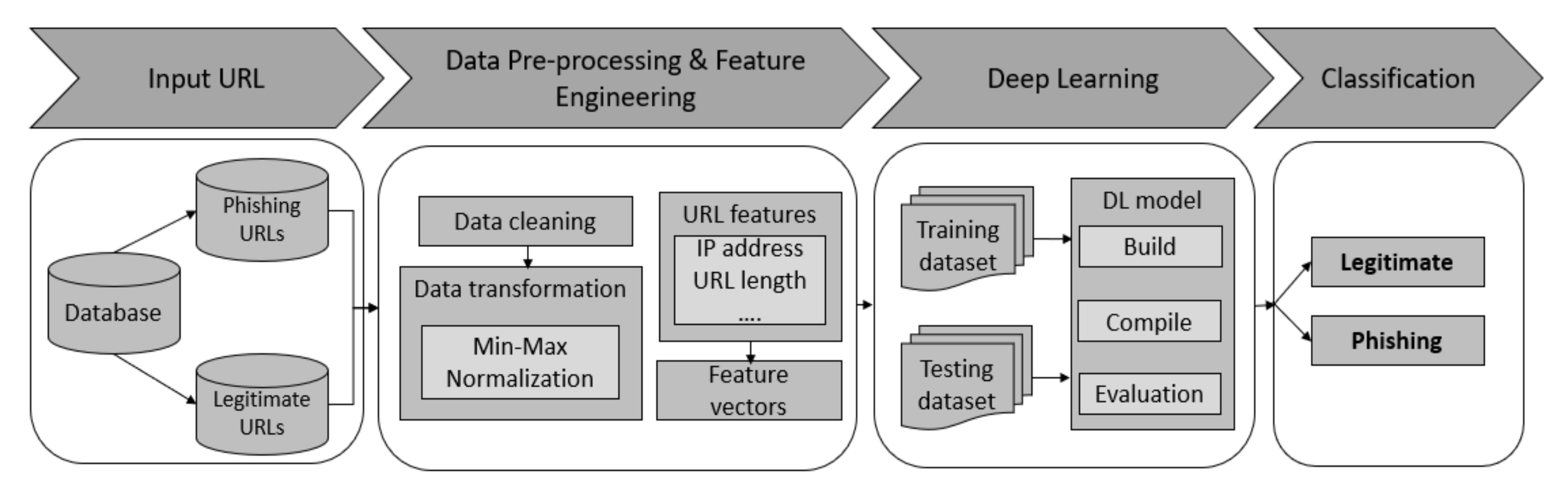
Figure 2 shows a theoretical workflow of the experimental setup for this empirical study. The entire process was divided into four stages: input URL (Uniform Resource Locator), data pre-processing and feature engineering, deep learning, and classification. In the first stage, a publicly available dataset was obtained from the University of California Irvine Machine Learning Repository (UCI), consisting of 11055 URLs. This dataset was comprised of both phishing and legitimate websites (4898 and 6157 URLs, respectively) [62]. In the second stage, the dataset went through a data cleaning and data transformation process in the pre-processing phase. Meanwhile, URL features were converted into feature vectors that acted as inputs to the DL model. The dataset was then split into two parts with a ratio of 8:2 (80% as training dataset and 20% as testing dataset). In the third stage, several DL algorithms were built, compiled, and evaluated. Finally, the webpage URL was classified as legitimate or phishing, and a set of performance metrics was measured to assess the performance of four DL models in detecting phishing websites.

In this research, Google Colaboratory, Python, and Tensorflow were used to build several DL models. Instead of running on a local machine and using local GPU, all four DL algorithms were trained using GPU on Google Colaboratory, with a capacity of 11.441MB. The programming language was written in Python code with the help of the TensorFlow package. The use of cloud servers allowed users to leverage the power of Google’s hardware to execute the codes and run Tensorflow operations. The dataset and source code used in the experiments are available on https://github.com/quangdn83/WebsitePhishingDetection (accessed on 21 September 2021) [63].

3.2. Website Features

In the experiment, website features were converted to feature vectors and used as inputs to DL models.

Table 4. List of phishing website features.

Type	No	Feature	Name	Description	Value
Address bar-based	1	IP address	UsingIP	Having IP address in URL	−1, 1
	2	URL length	LongURL	Long URL to hide the suspicious part	−1, 0, 1
	3	Shortening service	ShortURL	Using URL shortening services “TinyURL”	−1, 1
	4	@ Symbol	Symbol@	URL’s having @ symbol	−1, 1
	5	“//” redirecting	Redirecting//	Having “//” within URL path for directing	−1, 1
	6	Prefix suffix	PrefixSuffix	Adding prefix or suffix separated by (-) to the domain	−1, 1
	7	Sub domain	SubDomains	Sub domain and multi sub domain	−1, 0, 1
	8	SSL final state	HTTPS	Existence of HTTPS and validity of the certificate	−1, 0, 1
	9	Domain registration	DomainRegLen	Expiry date of domains/Domain registration length	−1, 1
	10	Favicon	Favicon	Favicon loaded from a domain	−1, 1
	11	Port	NonStdPort	Using non-standard port	−1, 1
	12	HTTPS token	HTTPSDomainURL	The existence of HTTPS token in the domain part of URL	−1, 1
Abnormal-based	13	Request URL	RequestURL	Request URL within a webpage/Abnormal request	−1, 1
	14	URL of anchor	AnchorURL	URL within <a> tag/Abnormal anchor	−1, 0, 1
	15	Links in tags	LinksInScriptTags	Links in <Meta>, <Script> and <Link> tags	−1, 0, 1
	16	SFH	ServerFormHandler	Server Form Handler	−1, 0, 1
	17	Email	InfoEmail	Submitting information to E-mail	−1, 1
	18	Abnormal URL	AbnormalURL	Host name is included in the URL/Whois	−1, 1
HTML and JavaScript-based	19	Redirecting	WebsiteForwarding	Number of times a website has been redirected	0, 1
	20	On mouseover	StatusBarCust	On mouse over changes status bar/Status bar customization	−1, 1
	21	Right click	DisableRightClick	Disabling right click	−1, 1
	22	Pop-up window	UsingPopupWindow	Using Pop-up window	−1, 1
	23	Iframe redirection	IframeRedirection	Using Iframe	−1, 1
Domain-based	24	Age of domain	AgeofDomain	Minimum age of a legitimate domain is 6 months	−1, 1
	25	DNS record	DNSRecording	Existence of DNS record for the domain	−1, 1
	26	Website traffic	WebsiteTraffic	Being among top 100,000 in Alexa rank	−1, 0, 1
	27	Page rank	PageRank	Having a page rank greater than 0.2	−1, 1
	28	Google index	GoogleIndex	Website indexed by Google	−1, 1
	29	Link reference	LinksPoitingToPage	Number of links pointing to a page	−1, 0, 1
	30	Statistical report	StatsReport	Top 10 domain and top 10 Ips from PhishTank	−1, 1
		Result	class	Phishing or legitimate	−1, 1

shows a list of 30 features used in this study. Each feature has three possible values: −1, 0, and 1 (−1 is phishing, 0 is suspicious, and 1 is benign). The last feature, named “class”, is the classification of the URL.

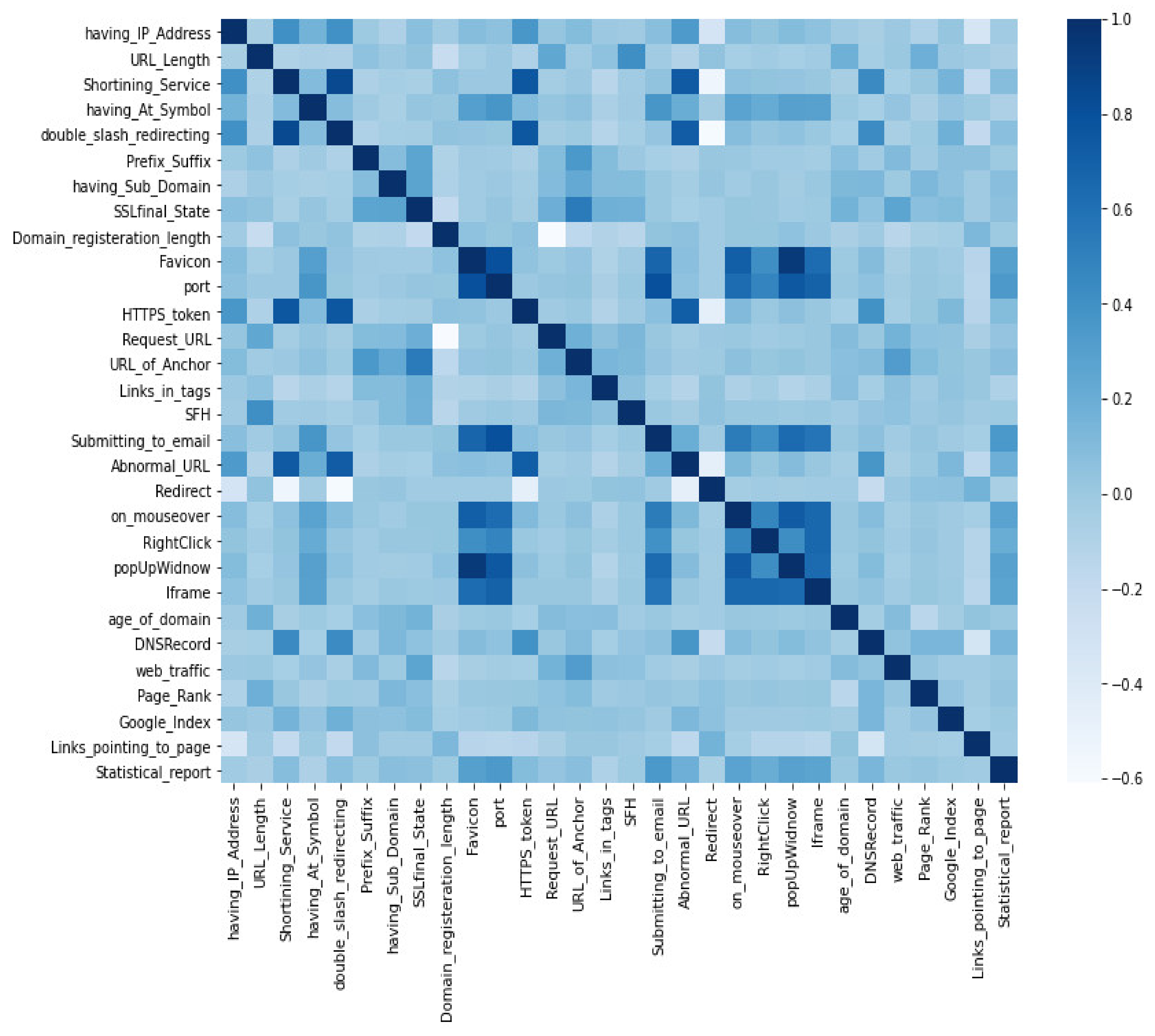
Figure 3 is the heatmap displaying the correlation matrix of these features. A standard range of correlation is from −1 to +1, where −1 is the lowest negative correlation, and +1 is the highest positive correlation. A negative correlation is displayed in the brighter color range, while a positive correlation is displayed in the darker color range. Particularly in this dataset, the mapping of two different features, named Favicon and popUpWindow, showed the darkest color, meaning they are highly or positively correlated. Positive correlations mean one feature marks the URL as phishing, and so does the other. Whereas negative correlations mean one feature marks the URL as malicious, while the other does not [6].

3.3. Deep Learning Models

This empirical study built four phishing detection models using four different DL algorithms: DNN, CNN, LSTM, and GRU. The general architecture of a typical DL-based phishing detection model consists of an input layer, one or more middle layers, and one output layer. Inputs to each DL model are website features that have already been converted to feature vectors. A total of 30 features were used in this study and hence, there were 30 neurons in the input layer of the neural network architecture. Different DL algorithms were used in the middle layers to build the phishing detection models, including DNN, CNN, LSTM, and GRU. Finally, only one neuron was used with a sigmoid activation function in the output layer to classify the web page as malicious or benign.

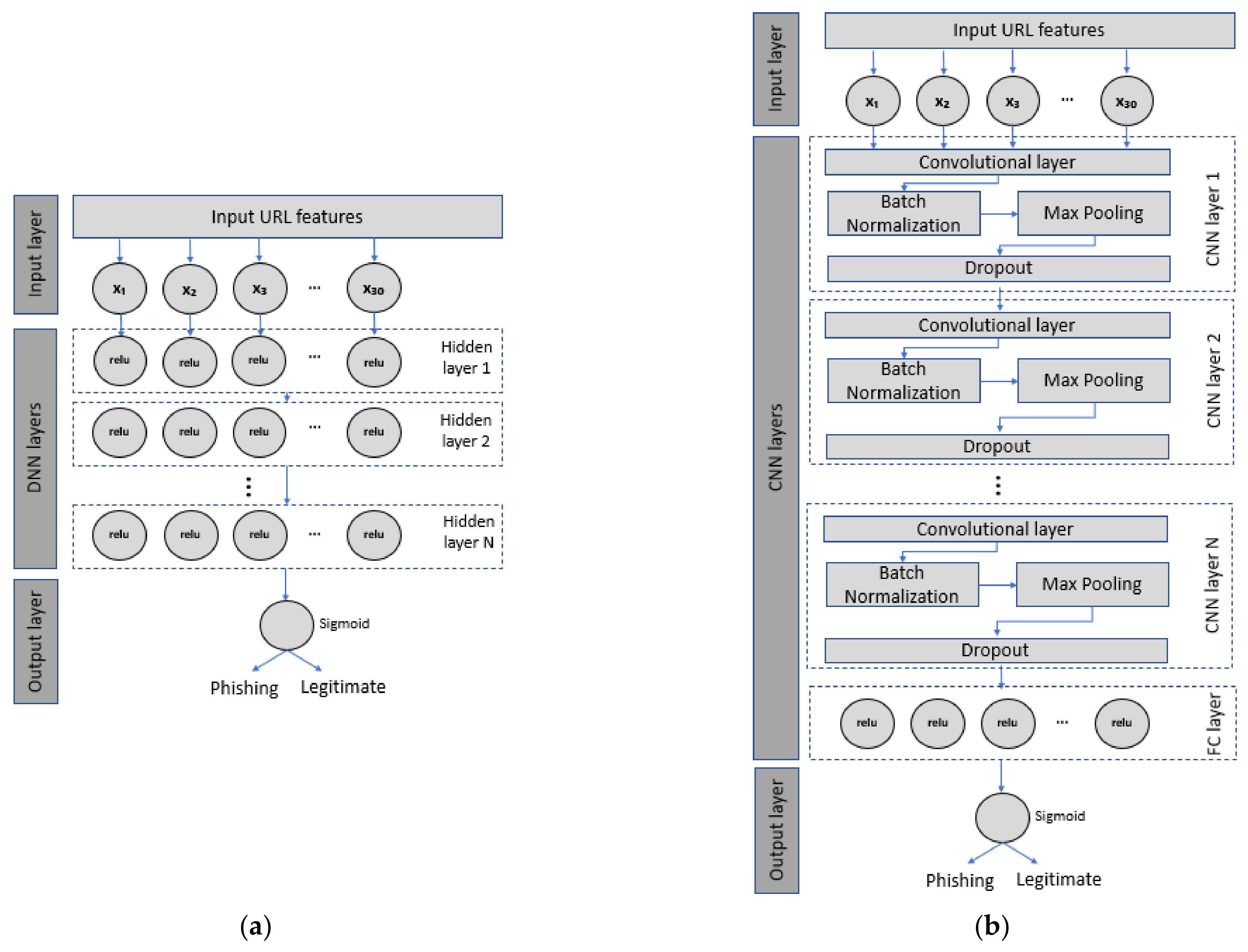
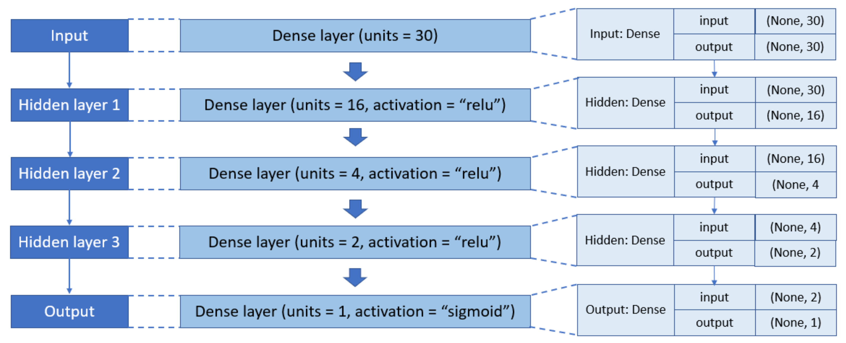
DNN. A DNN structure consists of an input layer, an output layer, and one or more hidden layers [18], as shown in Figure 4a. Each node or neuron in one layer is connected to the other nodes in the next layer to form a dense or fully-connected layer [19]. The number of hidden layers and neurons in each hidden layer can vary. The activation functions used in the hidden layers and the output layer are ReLU and sigmoid, respectively. Researchers need to fine-tune these parameters to find the optimal values that provide the highest detection accuracy.

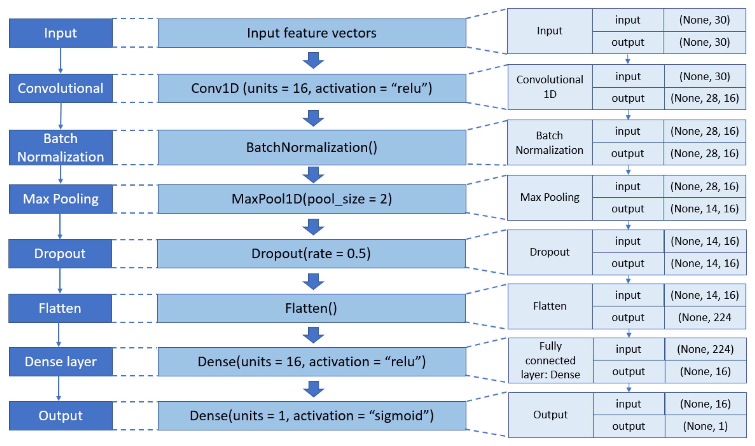
CNN. The architecture of a CNN model generally consists of three basic layers: a convolutional layer, a pooling layer, and a fully connected layer [37]. Firstly, a convolutional layer is used for feature extraction and consists of multiple convolutional kernels or filters that divide the input vectors into small blocks. Then, a series of feature maps are generated by performing convolutional operations on the input vectors with the chosen kernels [10]. Secondly, a pooling layer is utilized for dimensional reduction by reducing the dimensionality of the feature maps. The pooling layer has two functions: accelerate the network operation and improve the performance of the entire convolutional network [24]. Thirdly, a fully connected (FC) layer is responsible for classification purposes. FC layer is a traditional neural network that uses extracted features from previous layers to perform the final classification task [29]. To avoid overfitting problems, batch normalization and dropout strategies are used between CNN layers (Figure 4b). ReLU is utilized as an activation function in the convolutional and FC layers, while sigmoid is implemented in the output layer.

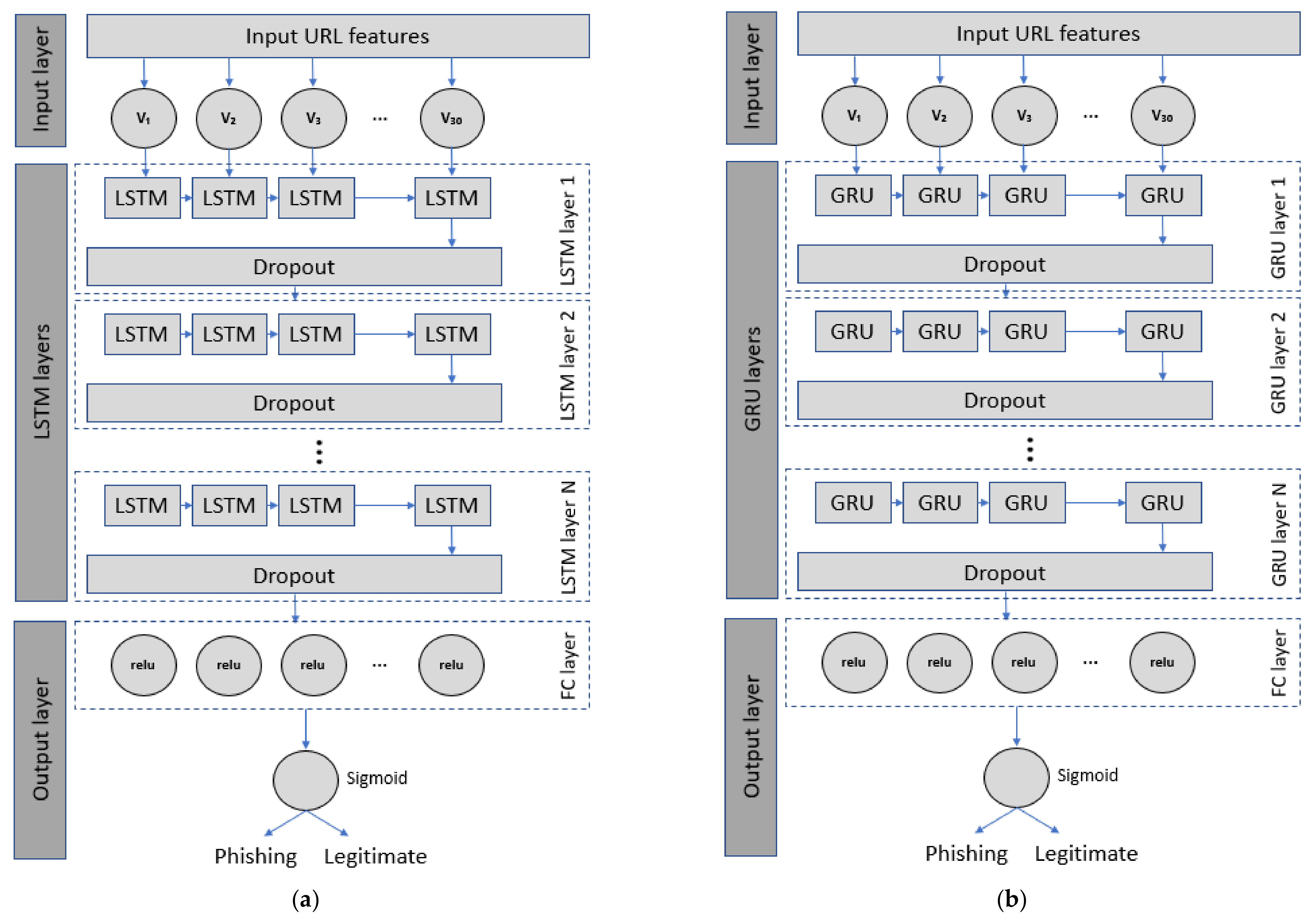
LSTM. LSTM is a variant of RNN which involves memory cell structure. The memory cell of a typical LSTM unit is comprised of three gates: an input gate, a forget gate, and an output gate [10]. Unlike a feedforward neural network, the output of a neuron in LSTM architecture at a particular instant can become input to the same neuron. There can be more than one LSTM layer in the LSTM-based phishing detection model, in which a dropout function is used in one layer after another to prevent overfitting issues as illustrated in Figure 5a. The LSTM and dense layers use ReLU, while the output layer uses Sigmoid as their activation functions.

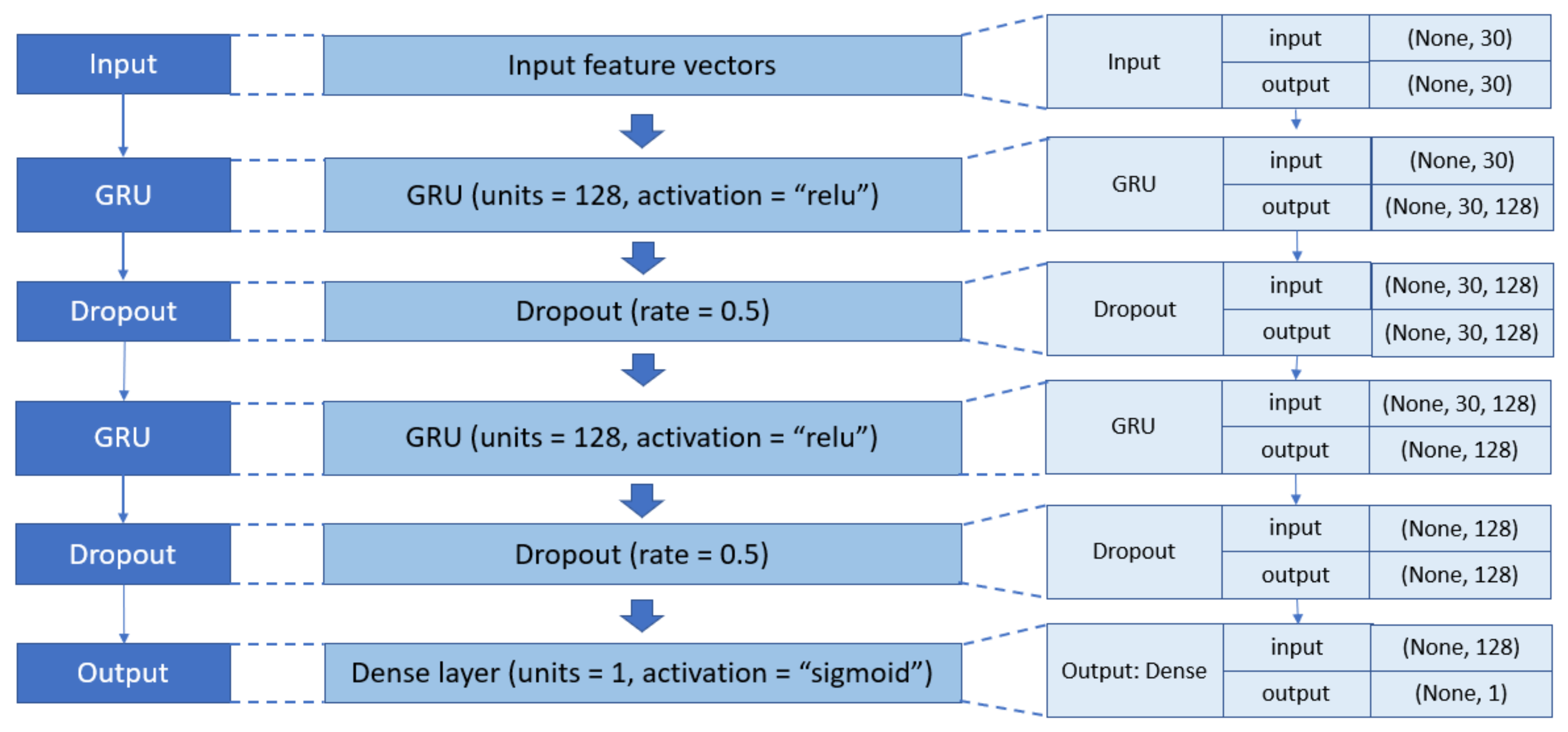
GRU. Similar to LSTM, GRU is constructed with gates and memory cells. Yet, it is simpler in implementation and computation [41]. Instead of a three-gate structure such as LSTM, there are only two gates in the GRU memory cell: input and forget gates. The overall architecture of GRU-based phishing detection models is similar to that of LSTM. Each GRU unit is replaced by an LSTM unit, as shown in Figure 5b.

3.4. Parameter Optimization

In designing and implementing four DL architectures, selecting a set of parameters that produce the best performance accuracy is essential. This process is called parameter tuning and was conducted through a series of experiments described as follows.

Experiment 1: Optimizing the learning rate. Firstly, a set of parameters (including the number of layers, number of neurons, number of kernels, kernel size, dropout rate, batch size, and number of epochs) was randomly selected for each DL algorithm. This set of parameters remained throughout the experiments, while the learning rate changed from 0.0001 to 0.1 to determine the value that yielded the highest detection accuracy.

Experiment 2: Optimizing the dropout rate. Using the learning rate found in the previous experiments, the impact of the dropout rate on the performance of various DL models was investigated. Different values of dropout rate were tested (from 0.1 to 0.5), and the rate with the best performance accuracy was recorded and used in the following experiments.

Experiment 3: Optimizing the neural network architecture. Since different network architectures might produce different results in detection accuracy, changing the structure of neural networks while keeping the learning rate and dropout rate constant was the next step in the parameter optimization process. Different layers, number of neurons per layer, number of kernels, and kernel sizes were examined to find the optimal set that offered the highest accuracy measure.

Experiment 4: Optimizing the batch size. With the learning rate, dropout rate, and deep neural network architecture obtained from the previous experiments, various values of batch size (from 8 to 1024) were tested, and their corresponding detection accuracies were measured. The batch size with the highest accuracy was used in the next experiment as part of parameter settings.

Experiment 5: Optimizing the number of epochs. The final step in the parameter tuning process was to optimize the number of epochs. The optimized value was determined by increasing the training iteration from 50 to 700. At this point, the optimal set of parameters that produced the best detection accuracy had been obtained. A list of parameters that affected the performance of four DL algorithms is recorded in

Table 5. List of parameters in various DL models.

DL Algorithm	Number of Layers	Number of Units	Number of Kernels	Kernel Size	Learning Rate	Dropout Rate	Batch Size	Number of Epochs
DNN
CNN
LSTM
GRU

.

Optimizer and activation functions. The parameters above vary according to the number of input features, the size of datasets, the type of DL algorithms, and the architecture of neural networks. Therefore, different authors in previous studies used different settings for their DL models. However, the common factor among them was the use of optimizer and activation functions. Most of the related studies utilized Adam as an optimizer, ReLU as an activation function for hidden or dense layer, and sigmoid as an activation function for the output layer.

Similarly, the same settings were used in the experimental setup of this empirical study without the need to fine-tune as in other hyper-parameters. Particularly, Adam was chosen because it proved to be the best optimizer among other optimization techniques. ReLU was selected as an activation function in the hidden layers of DNN, convolutional and fully connected layers in CNN, or LSTM/GRU layer in LSTM/GRU models. Finally, sigmoid was used as an activation function at the output layer because sigmoid function produces values in the range of 0 to 1. Thus, it is more suitable and adaptable for the phishing detection model [32] since phishing detection is a binary classification problem in which the output of the classifier is either 0 (phishing) or 1 (legitimate).

4. Results and Discussion

This section presents and discusses the results obtained from numerous experiments to examine the impact of hyperparameter tuning on the performance accuracy of four DL models. Various issues that arose from these experimental results are also highlighted to manifest the overlooked problems that need to be resolved. Moreover, this section also discusses the perspectives that motivate researchers to explore new directions in phishing detection and DL.

Results obtained from Experiment 1 to 5 described in Section 3.4 are provided in Appendix A as listed in

Table 6. List of experiments for parameter optimization in Appendix A.

Experiment	Description	Parameter	DL Algorithm
			DNN	CNN	LSTM	GRU
1	Optimizing the learning rate	Learning rate	Table A5	Table A9	Table A16	Table A21
2	Optimizing the dropout rate	Dropout rate	-	Table A10	Table A17	Table A22
3	Optimizing the neural network architecture	Number of layers/ Number of neurons per layer	Table A6	Table A13	Table A18	Table A23
		Number of kernels	-	Table A12	-	-
		Kernel size	-	Table A11	-	-
4	Optimizing the batch size	Batch size	Table A7	Table A14	Table A19	Table A24
5	Optimizing the number of epochs	Epoch	Table A8	Table A15	Table A20	Table A25

below.

After conducting a series of experiments, the optimal set of parameters with the highest performance accuracies for various DL models was summarized in

Table 7. An optimal set of parameter settings for various DL algorithms.

DL Algorithm	No of Layers	Number of Neurons	Number of Kernels	Kernel Size	Learning Rate	Dropout Rate	Batch Size	No of Epochs
DNN	5	(30 16 4 2 1)	-	-	0.001	-	32	500
CNN	4	(30 16 1)	16	3	0.005	0.5	32	50
LSTM	3	(30 128 1)	-	-	0.0005	0.5	32	700
GRU	4	(30 128 128 1)	-	-	0.001	0.5	32	200

. In the experiment setup, 30 website features were used as input vectors, hence, there were 30 neurons in the input layer of all four DL architectures. Furthermore, since phishing detection is a binary classification problem, only one neuron in the output layer could classify the URL as either legitimate or phishing.

4.1. Results with DNN

For the DNN algorithm (Figure 6), the neural network with three hidden layers and neurons of (16 4 2) (16 neurons in the first hidden layer, 4 neurons in the second hidden layer, and 2 neurons in the third hidden layer) achieved higher accuracy than other DNN architectures. Other parameters such as learning rate, batch size, and epoch were set to 0.001, 32, and 500, respectively. The highest accuracy recorded for this set of parameters was 97.29%. These results were achieved after a series of experiments provided in Appendix A (

Table A5. Performance metrics of DNN at different learning rate. (Architecture = (30 16 1), batch size = 32, epoch = 50).

Experiment (Exp.)	Learning Rate	FPR (%)	FNR (%)	Precision (%)	Recall (%)	F1-Score (%)	AUC (%)	Accuracy (%)	Time (s)
D1-1	0.0001	6.65	7.22	92.78	94.62	93.69	98.21	93.03	43
D1-2	0.0005	8.24	5.16	94.84	93.63	94.23	98.47	93.49	26
D1-3	0.001	5.11	4.63	95.37	96.06	95.71	98.97	95.16	45
D1-4	0.005	3.80	6.20	93.80	97.19	95.46	99.12	94.80	54
D1-5	0.01	6.95	4.32	95.68	94.27	94.97	98.58	94.48	53
D1-6	0.05	5.20	7.88	92.12	96.50	94.26	98.57	93.17	53
D1-7	0.1	6.35	7.76	92.24	94.98	93.59	98.01	92.85	54

,

Table A6. Performance metrics of different architectures of DNN. (Learning rate = 0.001, batch size = 32, epoch = 50).

Exp.	Hidden Layer	Neurons in Each Hidden Layer	FPR (%)	FNR (%)	Precision (%)	Recall (%)	F1-Score (%)	AUC (%)	Accuracy (%)	Time (s)
D2-1	1	(30 20 1)	5.88	5.96	94.04	95.35	94.69	99.00	94.08	53
D2-2		(30 16 1)	5.11	4.63	95.37	96.06	95.71	98.97	95.16	45
D2-3		(30 8 1)	5.86	4.40	95.60	95.67	95.64	98.85	94.98	52
D2-4	2	(30 20 16 1)	6.47	5.07	94.93	94.77	94.85	98.53	94.30	53
D2-5		(30 20 8 1)	5.69	4.38	95.62	95.30	95.46	99.06	95.02	51
D2-6		(30 20 4 1)	10.17	2.44	97.56	91.21	94.28	99.06	93.85	49
D2-7		(30 16 8 1)	6.61	3.63	96.37	94.66	95.51	99.03	95.03	36
D2-8		(30 16 4 1)	4.59	4.47	95.53	96.17	95.85	98.93	95.48	32
D2-9		(30 8 4 1)	7.69	4.22	95.78	93.49	94.62	98.89	94.17	50
D2-10	3	(30 20 16 8 1)	4.67	4.32	95.68	96.23	95.95	98.95	95.52	53
D2-11		(30 20 16 4 1)	10.08	2.72	97.28	91.12	94.10	98.83	93.71	53
D2-12		(30 20 16 2 1)	3.81	6.27	93.73	97.19	95.43	98.77	94.75	53
D2-13		(30 20 8 4 1)	4.68	5.43	94.57	96.47	95.51	98.82	94.89	23
D2-14		(30 20 8 2 1)	4.61	5.77	94.22	96.68	95.44	98.64	94.71	53
D2-15		(30 20 4 2 1)	9.82	3.21	96.79	91.89	94.27	98.74	93.71	53
D2-16		(30 16 8 4 1)	4.01	5.62	94.38	96.91	95.63	99.19	95.07	53
D2-17		(30 16 8 2 1)	3.64	5.17	94.83	97.27	96.03	99.11	95.48	53
D2-18		(30 16 4 2 1)	3.89	4.35	95.65	97.16	96.39	98.53	95.84	47
D2-19		(30 8 4 2 1)	7.55	3.00	97.00	93.47	95.20	99.04	94.84	52

,

Table A7. Performance metrics of DNN at different batch size. Architecture = [30 16 4 2 1], learning rate = 0.001, epoch = 50.

Experiment (Exp.)	Batch Size	FPR (%)	FNR (%)	Precision (%)	Recall (%)	F1-Score (%)	AUC (%)	Accuracy (%)	Time (s)
D3-1	8	4.23	5.40	94.60	96.63	95.60	99.00	95.12	124
D3-2	16	10.25	3.03	96.97	91.64	94.23	98.42	93.62	54
D3-3	32	3.89	4.35	95.65	97.16	96.39	98.53	95.84	47
D3-4	64	6.94	4.96	95.04	94.51	94.78	98.24	94.17	3
D3-5	128	4.52	5.87	94.13	96.50	95.30	98.33	94.71	3
D3-6	256	5.58	6.67	93.33	95.56	94.43	97.93	93.80	3
D3-7	512	6.20	6.67	93.33	95.22	94.27	98.56	93.53	3
D3-8	1024	7.57	7.06	92.94	93.93	93.44	96.52	92.72	3

and

Table A8. Performance metrics of DNN at different epochs. Architecture = [30 16 4 2 1], learning rate = 0.001, batch size = 32.

Experiment (Exp.)	Number of Epochs	FPR (%)	FNR (%)	Precision (%)	Recall (%)	F1-Score (%)	AUC (%)	Accuracy (%)	Time (s)
D4-1	50	3.89	4.35	95.65	97.16	96.39	98.53	95.84	47
D4-2	100	5.33	3.07	96.93	95.84	96.38	98.97	95.93	103
D4-3	150	3.29	5.43	94.57	97.48	96.00	98.97	95.48	153
D4-4	200	3.55	3.10	96.90	97.13	97.01	98.95	96.70	203
D4-5	250	2.63	4.92	95.08	97.96	96.50	99.08	96.07	253
D4-6	300	6.72	2.52	97.48	94.78	96.11	98.28	95.61	303
D4-7	500	3.01	2.47	97.53	97.53	97.53	99.40	97.29	503
D4-8	700	3.73	3.69	96.31	97.09	96.70	98.48	96.29	703

).

4.2. Results with CNN

Similar to the DNN algorithm, CNN also achieved the best detection accuracy with a batch size of 32. However, the CNN structure was different from that of DNN since the CNN model consisted of convolutional layers with a different number of kernels and kernel size (Figure 7). From the experiment, 16 kernels of size three (3) were found to have the highest accuracy of 96.56%. Other parameters, including learning rate, dropout rate, and epoch, were set to 0.005, 0.5, and 50, respectively. Results obtained from this set of experiments are provided in Appendix A (

Table A9. Performance metrics of CNN at different learning rates. (Number of kernels = 16, kernel size = 3, dropout rate = 0.5, batch size = 32, epoch = 50).

Experiment (Exp.)	Learning Rate	FPR (%)	FNR (%)	Precision (%)	Recall (%)	F1-Score (%)	AUC (%)	Accuracy (%)	Time (s)
C1-1	0.0001	5.23	6.65	93.35	96.18	94.75	98.31	93.94	52
C1-2	0.0005	5.18	5.75	94.25	96.32	95.27	98.92	94.48	53
C1-3	0.001	4.57	5.96	94.04	96.66	95.33	99.04	94.62	53
C1-4	0.005	3.50	3.39	96.61	97.09	96.85	99.51	96.56	54
C1-5	0.01	3.25	8.04	91.96	97.66	94.72	98.94	93.89	54
C1-6	0.05	16.34	3.94	96.06	85.13	90.27	97.32	89.78	53

,

Table A10. Performance metrics of CNN at different dropout rates. (Number of kernels = 16, kernel size = 3, learning rate = 0.005, batch size = 32, epoch = 50).

Experiment (Exp.)	Dropout Rate	FPR (%)	FNR (%)	Precision (%)	Recall (%)	F1-Score (%)	AUC (%)	Accuracy (%)	Time (s)
C5-1	0.1	5.31	2.98	97.02	95.40	96.21	99.36	95.93	54
C5-2	0.2	5.37	3.32	96.68	95.57	96.12	99.45	95.75	53
C5-3	0.3	3.53	5.36	94.64	97.20	95.90	99.21	95.43	81
C5-4	0.4	3.96	4.23	95.77	96.93	96.34	99.27	95.88	54
C5-5	0.5	3.50	3.39	96.61	97.09	96.85	99.51	96.56	54

,

Table A11. Performance metrics of CNN for different kernel sizes. (Number of kernels = 16, learning rate = 0.005, dropout rate = 0.5, batch size = 32, epoch = 50).

Experiment (Exp.)	Kernel Size	FPR (%)	FNR (%)	Precision (%)	Recall (%)	F1-Score (%)	AUC (%)	Accuracy (%)	Time (s)
C2-1	1	8.24	12.60	87.40	94.07	90.61	94.85	89.15	54
C2-2	2	6.00	9.81	90.19	95.50	92.77	97.81	91.77	53
C2-3	3	3.50	3.39	96.61	97.09	96.85	99.51	96.56	54
C2-4	4	3094	5.19	94.81	97.02	95.90	99.19	95.34	54
C2-5	5	6.42	3.50	96.50	94.96	95.72	99.30	95.21	53
C2-6	6	6.26	4.46	95.54	94.66	95.10	99.10	94.71	53

,

Table A12. Performance metrics of CNN for the different number of kernels. (Kernel size = 3, learning rate = 0.005, dropout rate = 0.5, batch size = 32, epoch = 50).

Experiment (Exp.)	Number of Kernels	FPR (%)	FNR (%)	Precision (%)	Recall (%)	F1-Score (%)	AUC (%)	Accuracy (%)	Time (s)
C3-1	8	3.41	6.61	93.39	97.51	95.41	98.81	94.71	54
C3-2	16	3.50	3.39	96.61	97.09	96.85	99.51	96.56	54
C3-3	32	4.87	5.29	94.71	96.31	95.50	99.24	94.89	54
C3-4	64	4.44	4.19	95.81	96.51	96.16	99.46	95.70	53
C3-5	128	3.01	5.70	94.30	97.73	95.99	99.28	95.43	153
C3-6	256	10.93	1.95	98.05	90.38	94.06	99.13	93.67	199
C3-7	512	6.56	4.56	95.44	94.57	95.00	98.96	94.53	253

,

Table A13. Performance metrics of different architectures of CNN. (Kernel size = 3, learning rate = 0.005, dropout rate = 0.5, batch size = 32, epoch = 50).

Exp.	Conv. Layer	Number of Kernels	FPR (%)	FNR (%)	Precision (%)	Recall (%)	F1-Score(%)	AUC (%)	Accuracy (%)	Time (s)
C6-1	1	64	4.44	4.19	95.81	96.51	96.16	99.46	95.70	53
C6-2		32	4.87	5.29	94.71	96.31	95.50	99.24	94.89	54
C6-3		16	3.50	3.39	96.61	97.09	96.85	99.51	96.56	54
C6-4		8	3.41	6.61	93.39	97.51	95.41	98.81	94.71	54
C6-5	2	(64 64)	0.83	10.97	89.03	99.43	93.94	99.05	92.90	108
C6-6		(64 32)	4.09	8.50	91.50	97.13	94.23	98.61	93.26	104
C6-7		(64 16)	2.63	10.71	89.29	97.97	93.43	98.34	92.63	104
C6-8		(64 8	5.13	7.42	92.58	96.22	94.37	98.63	93.53	103
C6-9		(32 32)	2.57	9.13	90.87	98.11	94.35	98.89	93.53	91
C6-10		(32 16)	6.14	8.06	91.94	95.25	93.57	98.34	92.76	104
C6-11		(32 8)	11.34	5.76	94.24	91.27	92.73	97.84	91.77	54
C6-12		(16 16)	6.22	8.37	91.63	94.87	93.22	97.97	92.58	53
C6-13		(16 8)	6.75	8.39	91.61	94.76	93.16	97.71	92.31	54
C6-14		(8 8)	8.42	10.02	89.98	93.81	91.85	96.58	90.64	54

,

Table A14. Performance metrics of CNN for different batch sizes. (Number of kernels = 16, kernel size =3, learning rate = 0.005, dropout rate = 0.5, epoch = 50).

Experiment (Exp.)	Batch Size	FPR (%)	FNR (%)	Precision (%)	Recall (%)	F1-Score (%)	AUC (%)	Accuracy (%)	Time (s)
C7-1	8	4.34	6.08	93.92	96.67	95.27	98.81	94.66	166
C7-2	16	3.64	5.63	94.37	97.26	95.79	99.19	95.21	85
C7-3	32	3.50	3.39	96.61	97.09	96.85	99.51	96.56	54
C7-4	64	4.94	6.05	93.95	96.04	94.99	98.83	94.44	54
C7-5	128	3.26	6.11	96.74	97.59	95.70	99.15	95.07	14
C7-6	256	3.31	4.95	95.05	97.50	96.26	99.29	95.75	8
C7-7	512	3.89	6.11	93.89	96.97	95.41	98.96	94.84	3
C7-8	1024	3.37	6.43	93.57	97.50	95.49	98.94	94.84	4

and

Table A15. Performance metrics of CNN for different number of epochs. (Number of kernels = 16, kernel size =3, learning rate = 0.005, dropout rate = 0.5, batch size = 32).

Experiment (Exp.)	Number of Epochs	FPR (%)	FNR (%)	Precision (%)	Recall (%)	F1-Score (%)	AUC (%)	Accuracy (%)	Time (s)
C8-1	50	3.50	3.39	96.61	97.09	96.85	99.51	96.56	54
C8-2	100	4.81	4.62	95.38	96.43	95.90	99.30	95.30	103
C8-3	150	2.93	5.18	94.82	97.70	96.24	99.32	95.79	153
C8-4	200	5.17	3.84	96.16	95.85	96.00	99.34	95.57	204
C8-5	250	3.63	4.97	95.03	97.13	96.07	99.29	95.61	254
C8-6	300	3.41	5.66	94.34	97.40	95.85	99.22	95.30	302
C8-7	500	4.57	4.16	95.84	96.31	96.08	99.28	95.66	503
C8-8	700	3.91	6.53	93.47	97.23	95.31	99.06	94.53	704

).

4.3. Results with LSTM

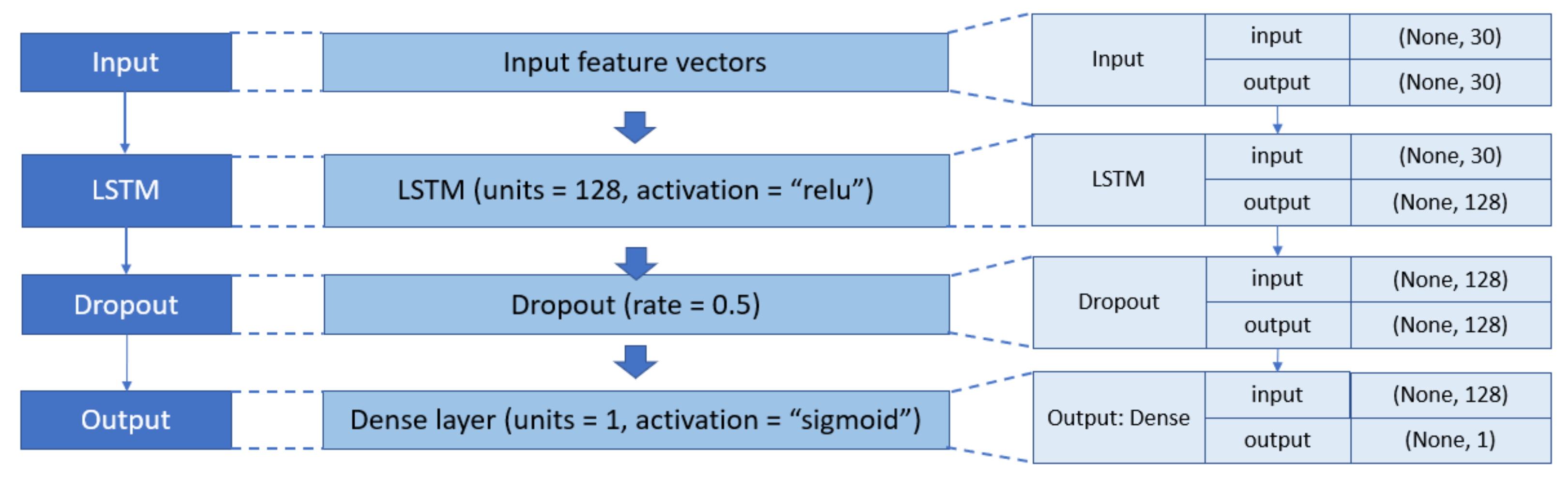
Likewise, different sets of parameters were tested for the LSTM model and provided in Appendix A (

Table A16. Performance metrics of LSTM at different learning rates. (Number of layers = 1, units = 128, dropout rate = 0.5, batch size = 32, epoch = 50).

Experiment (Exp.)	Learning Rate	FPR (%)	FNR (%)	Precision (%)	Recall (%)	F1-Score (%)	AUC (%)	Accuracy (%)	Time (min)
L1-1	0.0001	19.16	7.27	92.73	83.77	88.02	95.56	86.97	6.80
L1-2	0.0005	5.49	6.96	93.04	95.77	94.38	98.19	93.67	5.90
L1-3	0.001	14.82	6.64	93.36	87.12	90.13	97.01	89.42	6.72

,

Table A17. Performance metrics of LSTM at different dropout rates. (Number of layers = 1, units = 128, learning rate = 0.0005, batch size = 32, epoch = 50).

Experiment (Exp.)	Dropout Rate	FPR (%)	FNR (%)	Precision (%)	Recall (%)	F1-Score (%)	AUC (%)	Accuracy (%)	Time (min)
L2-1	0.1	8.28	8.12	91.88	93.86	92.86	97.24	91.81	6.23
L2-2	0.2	8.28	5.00	95.00	93.40	94.19	98.39	93.53	5.30
L2-3	0.3	7.84	6.33	93.67	93.59	93.63	98.13	92.99	6.75
L2-4	0.4	11.53	6.97	93.03	90.62	91.81	97.59	90.95	5.95
L2-5	0.5	5.49	6.96	93.04	95.77	94.38	98.19	93.67	5.90

,

Table A18. Performance metrics of different architectures of LSTM. (Learning rate = 0.0005, dropout rate = 0.5, batch size = 32, epoch = 50).

Exp.	No of Layer	Units per Layer	FPR (%)	FNR (%)	Precision (%)	Recall (%)	F1-Score (%)	AUC (%)	Accuracy (%)	Time (min)
L3-1	1	256	3.82	1047	89.53	97.34	93.27	98.27	92.13	19.78
L3-2		128	5.49	6.96	93.04	95.77	94.38	98.19	93.67	5.90
L3-3		64	12.42	5.34	94.66	88.74	91.61	97.32	91.18	3.40
L3-4		32	9.01	10.73	89.27	93.02	91.11	95.68	90.00	2.57
L3-5		16	12.57	14.32	85.68	90.10	87.83	93.85	86.43	2.57
L3-6	2	(128 128)	4.37	8.18	91.82	96.75	94.22	98.06	93.40	13.08
L3-7		(128 64)	6.88	7.57	92.43	95.00	93.70	97.79	92.72	10.97
L3-8		(128 32)	5.17	8.23	91.77	95.95	93.81	97.98	93.08	10.97
L3-9		(128 16)	9.61	5.93	94.07	91.82	92.93	98.22	92.36	8.87
L3-10	3	(128 128 128)	10.87	6.92	93.08	91.03	92.04	96.78	91.27	22.38
L3-11		(128 128 64)	6.46	7.27	92.73	95.06	93.88	98.06	93.08	20.40
L3-12		(128 128 32)	9.37	5.19	94.81	93.20	94.00	97.79	93.03	18.92
L3-13		(128 128 16)	12.17	6.80	93.20	89.96	91.55	97.33	90.73	15.92
L3-14		(128 64 64)	11.71	7.48	92.52	90.41	91.45	97.27	90.59	14.27
L3-15		(128 64 32)	8.70	7.05	92.95	93.10	93.03	97.62	92.22	14.73
L3-16		(128 64 16)	3.28	9.20	90.80	97.65	94.10	98.02	93.17	13.53
L3-17		(128 32 32)	3.48	9.19	90.81	97.61	94.09	98.25	93.03	12.48
L3-18		(128 32 16)	6.29	6.84	93.16	95.13	94.13	98.17	93.40	10.13
L3-19		(128 16 16)	4.66	8.17	91.83	96.63	94.17	97.95	93.26	10.50

,

Table A19. Performance metrics of LSTM for different batch sizes. (Number of layers = 1, units = 128, learning rate = 0.0005, dropout rate = 0.5, epoch = 50).

Experiment (Exp.)	Batch Size	FPR (%)	FNR (%)	Precision (%)	Recall (%)	F1-Score (%)	AUC (%)	Accuracy (%)	Time (min)
L4-1	8	6.70	6.03	93.97	94.44	94.21	98.35	93.67	18.53
L4-2	16	8.07	5.86	94.14	93.76	93.95	98.08	93.17	12.32
L4-3	32	5.49	6.96	93.04	95.77	94.38	98.19	93.67	5.90
L4-4	64	11.33	6.28	93.72	90.42	92.04	97.14	91.36	5.07
L4-5	128	4.10	15.08	84.92	97.31	90.70	96.34	88.92	4.22
L4-6	256	2.81	19.89	80.11	98.36	88.30	95.09	85.62	3.38

and

Table A20. Performance metrics of LSTM for the different number of epochs. (Number of layers = 1, units = 128, learning rate = 0.0005, dropout rate = 0.5, batch size = 32).

Experiment (Exp.)	Number of Epochs	FPR (%)	FNR (%)	Precision (%)	Recall (%)	F1-Score (%)	AUC (%)	Accuracy (%)	Time (min)
L5-1	50	5.49	6.96	93.04	95.77	94.38	98.19	93.67	5.90
L5-2	100	5.47	6.74	93.26	95.77	94.50	98.71	93.80	13.40
L5-3	150	3.86	8.51	91.49	97.15	94.23	98.05	93.40	20.42
L5-4	200	3.77	3.91	96.09	96.96	96.53	99.29	96.16	41.12
L5-5	250	3.28	4.90	95.10	97.49	96.28	99.23	95.79	54.23
L5-6	300	5.91	7.44	92.56	95.43	93.96	98.23	93.22	65.07
L5-7	500	2.97	4.18	95.82	97.75	96.77	98.54	96.34	120.27
L5-8	700	1.80	3.55	96.45	98.63	97.53	99.11	97.20	169.17

). The obtained results indicated that the same dropout rate (0.5) and batch size (32) were acquired to produce the highest performance accuracy (97.20%). Nevertheless, only one LSTM layer was needed in the network architecture (Figure 8) because the LSTM algorithm took longer to train. Therefore, adding more layers into the neural network only caused a high computation problem, which compromised the efficiency of the phishing detection system.

4.4. Results with GRU

Last but not least, parameter settings for the GRU algorithm were set to (30 128 128 1) (Figure 9), learning rate = 0.001, dropout rate = 0.5, batch size = 32, and epoch = 200. The highest accuracy that the model could achieve with this set of parameters was 96.70%. Detailed experiments of how to achieve this optimal set of parameters are provided in Appendix A (

Table A21. Performance metrics of GRU at different learning rates. (Number of layers = 1, units = 128, dropout rate = 0.5, batch size = 32, epoch = 50).

Experiment (Exp.)	Learning Rate	FPR (%)	FNR (%)	Precision (%)	Recall (%)	F1-Score (%)	AUC (%)	Accuracy (%)	Time (min)
G1-1	0.0001	14.64	7.21	92.79	88.14	90.40	95.99	89.37	5.45
G1-2	0.0005	6.36	7.51	92.49	95.00	93.73	98.39	92.99	6.40
G1-3	0.001	5.85	5.50	94.50	95.49	94.99	98.76	94.35	5.40
G1-4	0.005	4.90	9.03	90.97	96.18	93.50	97.74	92.72	6.42
G1-5	0.01	9.06	7.82	92.18	92.85	92.51	96.98	91.63	5.40

,

Table A22. Performance metrics of GRU at different dropout rates. (Number of layers = 1, units = 128, learning rate = 0.001, batch size = 32, epoch = 50).

Experiment (Exp.)	Dropout Rate	FPR (%)	FNR (%)	Precision (%)	Recall (%)	F1-Score (%)	AUC (%)	Accuracy (%)	Time (min)
G2-1	0.1	3.83	8.26	91.74	97.00	94.30	98.66	93.62	5.40
G2-2	0.2	7.61	5.55	94.45	93.91	94.18	98.81	93.53	6.42
G2-3	0.3	7.36	5.45	94.55	93.76	94.15	98.77	93.67	6.42
G2-4	0.4	7.72	6.01	93.99	94.22	94.10	98.50	93.26	5.40
G2-5	0.5	5.85	5.50	94.50	95.49	94.99	98.76	94.35	5.40

,

Table A23. Performance metrics of different architectures of GRU. (Learning rate = 0.001, dropout rate = 0.5, batch size = 32, epoch = 50).

Exp.	No of Layer	Units per Layer	FPR (%)	FNR (%)	Precision (%)	Recall (%)	F1-Score (%)	AUC (%)	Accuracy (%)	Time (min)
G3-1	1	256	5.18	6.27	93.73	95.89	94.80	98.94	94.21	10.40
G3-2		128	5.85	5.50	94.50	95.49	94.99	98.76	94.35	5.40
G3-3		64	6.05	7.61	92.39	95.09	93.72	98.02	93.08	4.42
G3-4		32	4.91	11.06	88.94	96.63	92.63	97.82	91.32	3.42
G3-5		16	7.61	5.86	94.14	93.76	93.95	98.11	93.35	2.98
G3-6	2	(128 128)	5.04	5.17	94.83	96.00	95.41	98.99	94.89	24.40
G3-7		(128 64)	6.01	5.78	94.22	95.29	94.75	98.80	94.12	22.40
G3-8		(128 32)	7.19	5.62	94.38	94.07	94.22	98.70	93.67	23.42
G3-9		(128 16)	5.32	6.37	93.63	95.97	94.78	98.71	94.08	22.42
G3-10	3	(128 128 128)	7.43	5.56	94.44	94.22	94.33	98.19	93.62	33.43
G3-11		(128 128 64)	10.23	3.60	96.40	91.71	94.00	98.61	93.35	32.87
G3-12		(128 128 32)	4.19	8.05	91.95	96.93	94.37	98.73	93.53	33.42
G3-13		(128 128 16)	7.76	5.72	94.28	94.13	94.20	98.67	93.40	34.43
G3-14		(128 64 64)	3.96	7.46	92.54	97.23	94.83	98.68	93.94	35.82
G3-15		(128 64 32)	4.07	7.05	92.95	96.90	94.88	98.92	94.21	33.32
G3-16		(128 64 16)	3.15	6.67	93.33	97.65	95.44	98.95	94.80	34.43
G3-17		(128 32 32)	6.12	6.33	93.67	95.33	94.49	98.67	93.76	12.43
G3-18		(128 32 16)	2.94	8.51	91.49	97.90	94.59	98.39	93.71	10.45
G3-19		(128 16 16)	9.84	4.34	95.66	91.67	93.62	98.77	93.08	11.45

,

Table A24. Performance metrics of GRU for different batch sizes. (Number of layers = 1, units = [128 128], learning rate = 0.001, dropout rate =0.5, epoch = 50).

Experiment (Exp.)	Batch Size	FPR (%)	FNR (%)	Precision (%)	Recall (%)	F1-Score (%)	AUC (%)	Accuracy (%)	Time (min)
G4-1	8	8.16	4.19	95.81	93.24	94.51	98.89	93.98	35.42
G4-2	16	2.28	10.51	89.49	98.35	93.71	98.67	92.76	17.42
G4-3	32	5.04	5.17	94.83	96.00	95.41	98.99	94.89	24.40
G4-4	64	1.63	12.26	87.74	98.83	92.96	98.93	91.86	11.43
G4-5	128	5.03	7.16	92.84	96.05	94.42	98.79	93.76	8.42
G4-6	256	4.59	6.99	93.01	96.50	94.72	98.36	94.03	6.42

and

Table A25. Performance metrics of GRU for a different number of epochs. (Number of units = [128 128], learning rate = 0.001, dropout rate = 0.5, batch size = 32).

Experiment (Exp.)	Number of Epochs	FPR (%)	FNR (%)	Precision (%)	Recall (%)	F1-Score (%)	AUC (%)	Accuracy (%)	Time (min)
G5-1	50	5.04	5.17	94.83	96.00	95.41	98.99	94.89	24.40
G5-2	100	3.54	4.69	95.31	97.37	96.33	98.84	95.79	16.42
G5-3	150	3.58	4.44	95.56	97.25	96.40	98.67	95.93	35.43
G5-4	200	2.48	3.94	96.06	98.03	97.04	98.79	96.70	55.07
G5-5	250	7.97	5.79	94.21	94.35	94.28	98.41	93.31	58.15
G5-6	300	5.80	4.75	95.25	95.63	95.44	98.79	94.80	83.43
G5-7	500	16.00	8.51	91.49	87.38	89.39	94.58	88.10	140.43
G5-8	700	50.70	42.55	57.45	73.51	64.50	48.79	55.09	205.00

). Similar to LSTM, GRU also required a long duration of training time. As a result, a more complex network architecture with more layers or neurons only increased the computational cost and reduced the model efficiency.

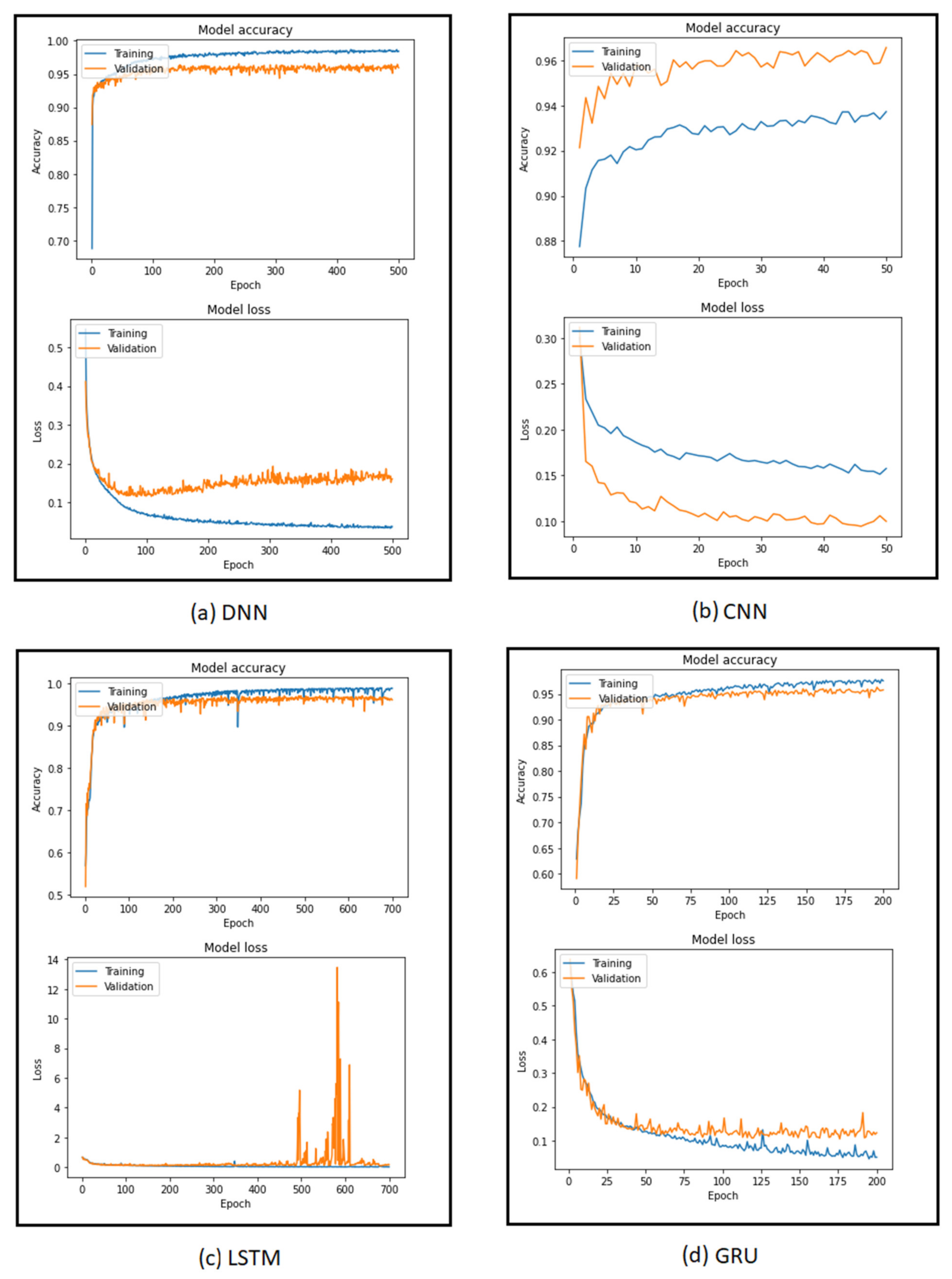
The loss and accuracy versus the number of epochs for different DL algorithms during training and validation are shown in Figure 10; as the number of epochs increased, the performance accuracy increased while the loss function decreased.

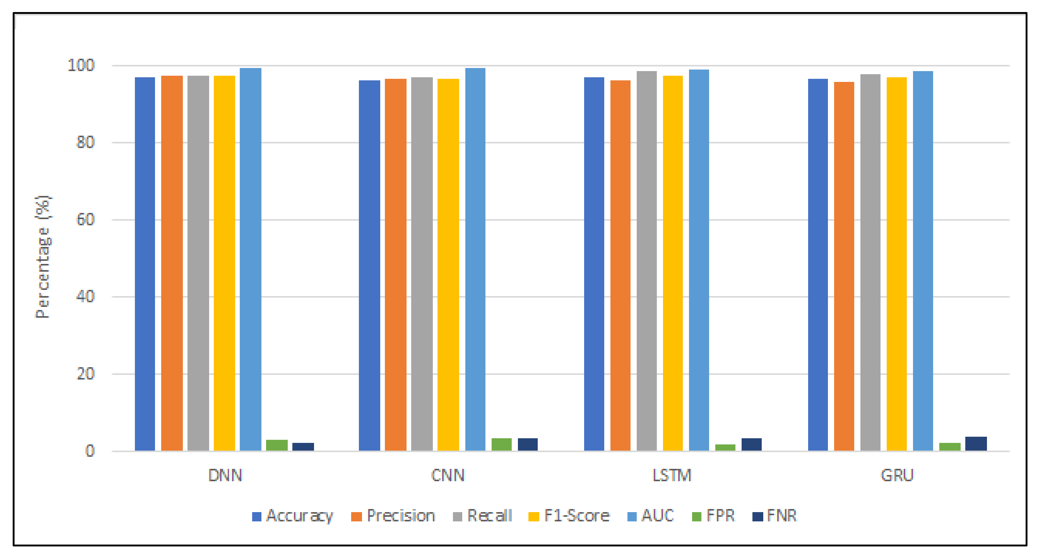
The performance metrics of four DL models are displayed in

Table 8. Performance metrics of four DL algorithms.

DL Algorithm	Performance Metrics
	FPR (%)	FNR (%)	ACC (%)	PR (%)	RC (%)	F1(%)	AUC (%)	Training Time (min)	Testing Time (s)	Parameter Size	Memory Storage (MB)
DNN	3.01	2.47	97.29	97.53	97.53	97.53	99.40	8.38	0.470	1507	172
CNN	3.50	3.39	96.56	96.61	97.09	96.85	99.51	0.9	0.263	3745	325
LSTM	1.80	3.55	97.20	96.45	98.63	97.53	99.11	169.17	0.804	66,689	184
GRU	2.48	3.94	96.70	96.06	98.03	97.04	98.79	55.07	1.447	149,505	184

and Figure 11. It is observed from the experiments that the accuracy of the DNN model was slightly higher than that of the other three DL algorithms. In addition, the amount of time required to train and test the DNN model was relatively low. DNN also had the smallest parameter size and occupied the least memory storage. In contrast, CNN had the lowest measure for accuracy compared with the other three DL mechanisms, yet it required the shortest duration for model training and testing. The parameter size for CNN was more significant than that for DNN, but CNN consumed the most computational power in terms of GPU storage.

Meanwhile, to achieve an almost equivalent accuracy level as DNN, many iterations were involved in the training phase of LSTM and GRU models, which made their training time longer than the others. As the number of neurons in LSTM and GRU models was higher, their parameters were also more significant. However, the GPU capacity requirement for LSTM and GRU was less than that for CNN. To sum up, no DL algorithm provided the best measure across all performance metrics. Each DL technique has its pros and cons; therefore, selecting an appropriate DL approach is a challenging task that can affect the outcomes of a phishing detection model.

In

Table 9. Comparison of parameter settings with other studies using the same dataset.

Reference	DL Algorithm	Parameter Settings									ACC (%)
		Learning Rate	Input Layer	Hidden Layer	Output Layer	Number of Kernels	Kernel Size	Dropout Rate	Batch Size	Epoch
[18]	DNN	0.01	30	(20 10 5)	2	-	-	-	-	200	97.50
[28]	CNN	-	30	(64 64)	1	64/64	12/6	-	-	220	97.20
[6]	MLP	-	-	(100 100)	-	-	-	-	-	-	96.65
[64]	DNN.BA 1	0.0185	30	(50 30)	2	-	-	-	44	155	95.76
	DNN.HBA 2	0.0462	30	(42 30)	2	-	-	-	101	135	95.00
	DNN.FA 3	0.0053	30	(50 30)	2	-	-	-	37	192	96.65
Our study	DNN CNN LSTM GRU	0.001 0.005 0.0005 0.001	30 30 30 30	(16 4 2) (16) (128) (128 128)	1 1 1 1	- 16 - -	- 3 - -	- 0.5 0.5 0.5	32 32 32 32	500 50 700 200	97.29 96.56 97.20 96.70

¹ Parameter settings for DNN using Bat Algorithm. ² Parameter settings for DNN using Hybrid Bat Algorithm. ³ Parameter settings for DNN using Firefly Algorithm.

, results obtained from the empirical analysis of this study are compared with those attained from other authors using the same dataset. In previous studies, the authors used only one type of DL algorithm, such as DNN, CNN, or MLP (multi-layer perceptron). However, four different DL architectures from various categories (supervised, unsupervised, and hybrid) were implemented in our research work. Moreover, dropout rate and batch size, which were not specified in some studies [6,18,28], were included in our empirical analysis. In addition, it is also observed from the table that although different authors used the same algorithm, their optimal set of parameters and accuracy results were not the same. This implies that researchers still had to perform manual parameter tuning to obtain the optimal parameter settings for their DL models. The authors in [64] suggested that this process could be optimized using swarm intelligence (Bat, Hybrid Bat, and Firefly Algorithm). Yet, their accuracy measures were either equivalent or lower than other authors. Meanwhile, the accuracies obtained from our study are almost as high as other authors. Moreover, we also measured additional metrics to obtain a more comprehensive analysis of different DL algorithms’ performance in detecting phishing websites.

Table 10. Comparison of performance metrics with other studies using the same dataset.

Ref.	DL Algorithm	Performance Metrics
		Conventional							Additional
		FPR (%)	FNR (%)	ACC (%)	PR (%)	RC (%)	F1 (%)	AUC (%)	Training Time (min)	Testing Time (s)	Parameter size	Memory Storage (MB)
[18]	DNN	1.80	3.30	97.50	97.70	96.70	97.20	-	-	-	-	-
[28]	CNN	-	-	97.20	96.90	98.10	97.50	-	10.67	0.472	27,985	-
[6]	MLP	-	-	96.65	96.65	96.65	96.65	-	-	-	-	-
[64]	DNN.BA 1	-	-	95.76	-	-	95.70	-	-	-	-	-
	DNN.HBA 2	-	-	95.00	-	-	94.93	-	-	-	-	-
	DNN.FA 3	-	-	96.65	-	-	96.61	-	-	-	-	-
Our study	DNN	3.01	2.47	97.29	97.53	97.53	97.53	99.40	8.38	0.470	1,507	172
	CNN	3.50	3.39	96.56	96.61	97.09	96.85	99.51	0.9	0.263	3,745	325
	LSTM	1.80	3.55	97.20	96.45	98.63	97.53	99.11	169.17	0.804	66,689	184
	GRU	2.48	3.94	96.70	96.06	98.03	97.04	98.79	55.07	1.447	149,505	184

¹ Parameter settings for DNN using Bat Algorithm. ² Parameter settings for DNN using Hybrid Bat Algorithm. ³ Parameter settings for DNN using Firefly Algorithm.

provides a comparison of various performance metrics between our research work and previous studies using the same dataset. Compared with [64], our study achieved higher accuracy and F1-Score for DNN and included various metrics not measured in [64]. Since MLP is a subset of DNN, MLP results from [6] could be compared with DNN from our empirical analysis. The obtained results showed that our DNN model outperformed the MLP algorithm in all four metrics: ACC, PR, RC, and F1-Score. In addition, although DNN and CNN accuracies in [18,28] demonstrated slightly better results than ours, some of the performance metrics were not calculated in these studies. In [18], for instance, AUC, time complexity, and memory constraints were not included in the evaluation process. Even though training time, testing time, and parameter size were measured in [28], other metrics (FPR, FNR, AUC, and memory storage) were not reported.

On the contrary, our study provided a complete set of performance metrics for four different DL algorithms. Conventional metrics (FPR, FNR, ACC, PR, RC, F1, and AUC) were used to evaluate the effectiveness of the DL mechanism in detecting phishing websites. In contrast, additional metrics (training time, testing time, parameter size, and memory usage) were utilized to assess the computational complexity of the phishing detection model.

4.5. Issues and Perspectives

Parameter Tuning. It can be observed from the experiments that parameter tuning is the common problem among all four DL algorithms. The parameters in the DL models consist of the number of layers in the neural networks, number of neurons (units) in each layer, number of kernels and kernel size (for CNN), learning rate, dropout rate, number of epochs, batch size, etc. [17]. There is no standard and specific guideline for setting these parameters so that the highest performance accuracy can be achieved. Manual fine-tuning and conducting a series of experiments through trial and error are standard practices among researchers who work with DL models. However, this process is tedious, time-consuming, and labor-intensive. One possible solution to overcome the problem of manual parameter tuning is to use optimization techniques to fine-tune the parameters and shorten the tuning process [64].

Accuracy Deficiency. Accuracy deficiency is another widespread issue among DL models, as accuracy is one of the most critical metrics that are used to evaluate the performance of the selected DL algorithm. Several factors affect the accuracy of a phishing detection model, including the quality of the dataset, the extracted features, the chosen classifier, the parameter settings, etc. Some of the current studies in the literature focused on solving the problem of accuracy deficiency by applying the existing DL algorithms [6,7,43]. In contrast, other researchers combined multiple DL techniques in an ensemble model to enhance the detection accuracy [11,31,37]. Ensemble DL (EDL) models are formed by stacking various DL algorithms in parallel and are divided into two categories: homogeneous and heterogeneous. A homogeneous EDL architecture is constructed by combining DL algorithms of the same type (CNN-CNN, LSTM-LSTM, GRU-GRU, etc.). In contrast, a heterogeneous EDL model incorporates DL mechanisms of different kinds (CNN-LSTM, CNN-GRU, LSTM-GRU, etc.). By doing so, the strengths of individual algorithms are merged while their weaknesses are resolved.

Computation Complexity. Computational complexity is another factor that needs to be considered in the design and implementation of DL architecture. Computational complexity can be divided into time complexity and memory constraints. Time complexity involves training and testing, while memory constraints refer to the parameter size and GPU storage capacity. DL generally requires a massive amount of data and substantial training time [65]. Although DL performs better than traditional machine learning on larger datasets, training with a large amount of data is also challenging and time-consuming. Since big datasets might consist of millions of instances, a longer time is needed to train the neural network to achieve high-performance accuracy.

Moreover, limited processing and storage facilities might also cause a delay in the training duration of a DL model [2]. Therefore, selecting an appropriate DL algorithm that can produce maximum accuracy with a minimum amount of time and computational consumption is essential. Plus, reducing the complexity of neural network architecture is also an alternative that can be applied to decrease training time. Last but not least, big data or cloud-based technologies can be integrated with DL to enhance the processing and storage capabilities, leading to a more robust and efficient model for phishing detection.

5. Conclusions and Future Works

In conclusion, many different DL algorithms exist, which numerous researchers in previous studies have implemented to detect phishing websites. However, choosing the right approach best suited for a specific application or dataset is a challenging task. To solve this problem, an empirical study was conducted in this paper, based on some of the most frequently-used DL techniques, such as DNN, CNN, LSTM, and GRU. Different neural network architectures were tested for each of these DL algorithms to find the optimal set of parameter settings that produce the highest performance accuracy. The empirical experiments were performed on the UCI dataset, consisting of 11055 phishing and benign URLs with 30 website features. Various performance metrics were measured to evaluate the effectiveness and the feasibility of the DL-based phishing detection model. The results obtained from the experiments indicated that among the four DL techniques, there was no single algorithm that produced the best measures in all performance metrics. Researchers and developers need to select the best suited to their particular applications or according to specific requirements. They can also combine different DL algorithms in a hybrid or ensemble model to join their advantages and cure their disadvantages.

As part of our future work, we plan to experiment with other DL algorithms that are relatively new and have not been fully explored in the phishing detection domain, such as Autoencoder (AE), Generative Adversarial Network (GAN), or Deep Reinforcement Learning (DRL). In addition to homogeneous EDL models, we will also implement heterogeneous EDL architectures by integrating multiple DL algorithms of different genres. Plus, we plan to use a more significant and unbalanced dataset in the experiment set up to reflect real-life scenarios, as we live in a big data era and phishing is an imbalanced classification problem, where the number of phishing URLs is much smaller than legitimate URLs.

References

- Ahmad, R.; Alsmadi, I. Machine learning approaches to IoT security: A systematic literature review. Internet Things 2021, 14, 100365. [Google Scholar] [CrossRef]
- Amanullah, M.A.; Habeeb, R.A.A.; Nasaruddin, F.H.; Gani, A.; Ahmed, E.; Nainar, A.S.M.; Akim, N.M.; Imran, M. Deep learning and big data technologies for IoT security. Comput. Commun. 2020, 151, 495–517. [Google Scholar] [CrossRef]
- Liu, H.; Lang, B. Machine Learning and Deep Learning Methods for Intrusion Detection Systems: A Survey. Appl. Sci. 2019, 9, 4396. [Google Scholar] [CrossRef] [Green Version]
- Asharf, J.; Moustafa, N.; Khurshid, H.; Debie, E.; Haider, W.; Wahab, A. A Review of Intrusion Detection Systems Using Machine and Deep Learning in Internet of Things: Challenges, Solutions and Future Directions. Electronics 2020, 9, 1177. [Google Scholar] [CrossRef]
- Bello, I.; Chiroma, H.; Abdullahi, U.A.; Gital, A.Y.; Jauro, F.; Khan, A.; Okesola, J.O.; Abdulhamid, S.M. Detecting ransomware attacks using intelligent algorithms: Recent development and next direction from deep learning and big data perspectives. J. Ambient Intell. Humaniz. Comput. 2020, 12, 8699–8717. [Google Scholar] [CrossRef]
- Al-Ahmadi, S. PDMLP: Phishing Detection Using Multilayer Perceptron. Int. J. Netw. Secur. Its Appl. 2020, 12. SSRN:3624621. Available online: https://papers.ssrn.com/abstract=3624621 (accessed on 12 May 2021). [CrossRef]
- Aljofey, A.; Jiang, Q.; Qu, Q.; Huang, M.; Niyigena, J.-P. An Effective Phishing Detection Model Based on Character Level Convolutional Neural Network from URL. Electronics 2020, 9, 1514. [Google Scholar] [CrossRef]
- Al-Milli, N.; Hammo, B.H. A Convolutional Neural Network Model to Detect Illegitimate URLs. In Proceedings of the 2020 11th International Conference on Information and Communication Systems (ICICS), Irbid, Jordan, 7–9 April 2020; pp. 220–225. [Google Scholar] [CrossRef]
- Feng, J.; Zou, L.; Nan, T. A Phishing Webpage Detection Method Based on Stacked Autoencoder and Correlation Coefficients. J. Comput. Inf. Technol. 2019, 27. [Google Scholar] [CrossRef]
- Feng, J.; Zou, L.; Ye, O.; Han, J. Web2Vec: Phishing Webpage Detection Method Based on Multidimensional Features Driven by Deep Learning. IEEE Access 2020, 8, 221214–221224. [Google Scholar] [CrossRef]
- Huang, Y.; Yang, Q.; Qin, J.; Wen, W. Phishing URL Detection via CNN and Attention-Based Hierarchical RNN. In Proceedings of the 2019 18th IEEE International Conference on Trust, Security and Privacy in Computing and Communications/13th IEEE International Conference on Big Data Science And Engineering (TrustCom/BigDataSE), Rotorua, New Zealand, 5–8 August 2019; pp. 112–119. [Google Scholar] [CrossRef]
- Chen, Z. Deep Learning for Cybersecurity: A Review. In Proceedings of the 2020 International Conference on Computing and Data Science (CDS), Stanford, CA, USA, 1–2 August 2020; pp. 7–18. [Google Scholar]
- Naway, A.; LI, Y. A Review on The Use of Deep Learning in Android Malware Detection. arXiv 2018, arXiv:181210360. Available online: http://arxiv.org/abs/1812.10360 (accessed on 3 April 2021).
- Sarker, I.H. Deep Cybersecurity: A Comprehensive Overview from Neural Network and Deep Learning Perspective. SN Comput. Sci. 2021, 2, 154. [Google Scholar] [CrossRef]
- Quang, D.N.; Selamat, A.; Krejcar, O. Recent Research on Phishing Detection Through Machine Learning Algorithm. In Advances and Trends in Artificial Intelligence. Artificial Intelligence Practices; Fujita, H., Selamat, A., Lin, J.C.-W., Ali, M., Eds.; Springer International Publishing: Cham, Switzerland, 2021; pp. 495–508. [Google Scholar]
- Wu, Y.; Wei, D.; Feng, J. Network Attacks Detection Methods Based on Deep Learning Techniques: A Survey. Secur. Commun. Netw. 2020, 2020, e8872923. [Google Scholar] [CrossRef]
- Mahdavifar, S.; Ghorbani, A.A. Application of deep learning to cybersecurity: A survey. Neurocomputing 2019, 347, 149–176. [Google Scholar] [CrossRef]
- Mahdavifar, S.; Ghorbani, A.A. DeNNeS: Deep embedded neural network expert system for detecting cyber attacks. Neural Comput. Appl. 2020, 32, 14753–14780. [Google Scholar] [CrossRef]
- Sahingoz, O.K.; Işılay Baykal, S.; Bulut, D. Phishing detection from urls by using neural networks. In Computer Science & Information Technology (CS & IT); AIRCC Publishing Corporation: Chennai, India, 2018; pp. 41–54. [Google Scholar] [CrossRef]
- Khan, M.F.; Al, E. Detection of Phishing Websites Using Deep Learning Techniques. Turk. J. Comput. Math. Educ. TURCOMAT 2021, 12, 3880–3892. [Google Scholar] [CrossRef]
- Sountharrajan, S.; Nivashini, M.; Shandilya, S.K.; Suganya, E.; Bazila Banu, A.; Karthiga, M. Dynamic Recognition of Phishing URLs Using Deep Learning Techniques. In Advances in Cyber Security Analytics and Decision Systems; Shandilya, S.K., Wagner, N., Nagar, A.K., Eds.; EAI/Springer Innovations in Communication and Computing; Springer International Publishing: Cham, Switzerland, 2020; pp. 27–56. ISBN 978-3-030-19353-9. [Google Scholar] [CrossRef]
- Selvaganapathy, S.; Nivaashini, M.; Natarajan, H. Deep belief network based detection and categorization of malicious URLs. Inf. Secur. J. Glob. Perspect. 2018, 27, 145–161. [Google Scholar] [CrossRef]
- Aldweesh, A.; Derhab, A.; Emam, A.Z. Deep learning approaches for anomaly-based intrusion detection systems: A survey, taxonomy, and open issues. Knowl.-Based Syst. 2020, 189, 105124. [Google Scholar] [CrossRef]
- Wei, W.; Ke, Q.; Nowak, J.; Korytkowski, M.; Scherer, R.; Woźniak, M. Accurate and fast URL phishing detector: A convolutional neural network approach. Comput. Netw. 2020, 178, 107275. [Google Scholar] [CrossRef]
- Liu, D.; Lee, J.-H.; Wang, W.; Wang, Y. Malicious Websites Detection via CNN based Screenshot Recognition. In Proceedings of the 2019 International Conference on Intelligent Computing and its Emerging Applications (ICEA), Tainan, Taiwan, 30 August–1 September 2019; pp. 115–119. [Google Scholar] [CrossRef]
- Phoka, T.; Suthaphan, P. Image Based Phishing Detection Using Transfer Learning. In Proceedings of the 2019 11th International Conference on Knowledge and Smart Technology (KST), Phuket, Thailand, 23–26 January 2019; pp. 232–237. [Google Scholar] [CrossRef]
- Xiao, X.; Zhang, D.; Hu, G.; Jiang, Y.; Xia, S. CNN–MHSA: A Convolutional Neural Network and multi-head self-attention combined approach for detecting phishing websites. Neural Netw. 2020, 125, 303–312. [Google Scholar] [CrossRef] [PubMed]
- Yerima, S.Y.; Alzaylaee, M.K. High Accuracy Phishing Detection Based on Convolutional Neural Networks. In Proceedings of the 2020 3rd International Conference on Computer Applications Information Security (ICCAIS), Riyadh, Saudi Arabia, 19–21 March 2020; pp. 1–6. [Google Scholar] [CrossRef]
- Wang, H.; Yu, L.; Tian, S.; Peng, Y.; Pei, X. Bidirectional LSTM Malicious webpages detection algorithm based on convolutional neural network and independent recurrent neural network. Appl. Intell. 2019, 49, 3016–3026. [Google Scholar] [CrossRef]
- Rasymas, T.; Dovydaitis, L. Detection of phishing URLs by using deep learning approach and multiple features combinations. Balt. J. Mod. Comput. 2020, 8, 471–483. [Google Scholar] [CrossRef]
- Srinivasan, S.; Vinayakumar, R.; Arunachalam, A.; Alazab, M.; Soman, K. DURLD: Malicious URL Detection Using Deep Learning-Based Character Level Representations. In Malware Analysis Using Artificial Intelligence and Deep Learning; Stamp, M., Alazab, M., Shalaginov, A., Eds.; Springer International Publishing: Cham, Switzerland, 2021; pp. 535–554. ISBN 978-3-030-62582-5. [Google Scholar] [CrossRef]
- Wang, W.; Zhang, F.; Luo, X.; Zhang, S. PDRCNN: Precise Phishing Detection with Recurrent Convolutional Neural Networks. Secur. Commun. Netw. 2019, 2019, e2595794. [Google Scholar] [CrossRef]
- Yang, P.; Zhao, G.; Zeng, P. Phishing Website Detection Based on Multidimensional Features Driven by Deep Learning. IEEE Access 2019, 7, 15196–15209. [Google Scholar] [CrossRef]
- Yang, W.; Zuo, W.; Cui, B. Detecting Malicious URLs via a Keyword-Based Convolutional Gated-Recurrent-Unit Neural Network. IEEE Access 2019, 7, 29891–29900. [Google Scholar] [CrossRef]
- M, Y.V.; Janet, B.; Reddy, S. Anti-phishing System using LSTM and CNN. In Proceedings of the 2020 IEEE International Conference for Innovation in Technology (INOCON), Bangluru, India, 6–8 November 2020; pp. 1–5. [Google Scholar] [CrossRef]
- jaysinha. Available online: https://jaysinha.me/files/phishx_preprint.pdf (accessed on 18 September 2021).
- Al-Ahmadi, S. A Deep Learning Technique for Web Phishing Detection Combined URL Features and Visual Similarity. Soc. Sci. Res. Netw. 2020. SSRN:3716033. Available online: https://papers.ssrn.com/abstract=3716033 (accessed on 10 March 2021). [CrossRef]
- Zhang, Q.; Bu, Y.; Chen, B.; Zhang, S.; Lu, X. Research on phishing webpage detection technology based on CNN-BiLSTM algorithm. J. Phys. Conf. Ser. 2021, 1738, 012131. [Google Scholar] [CrossRef]
- Chen, D.; Wawrzynski, P.; Lv, Z. Cyber security in smart cities: A review of deep learning-based applications and case studies. Sustain. Cities Soc. 2021, 66, 102655. [Google Scholar] [CrossRef]
- Elnagar, S.; Thomas, M. A Cognitive Framework for Detecting Phishing Websites. In Proceedings of the International Conference on Advances on Applied Cognitive Computing (ACC 2018), Las Vegas, NV, USA, 30 July–2 August 2018; pp. 60–61. [Google Scholar]
- Feng, T.; Yue, C. Visualizing and Interpreting RNN Models in URL-based Phishing Detection. In Proceedings of the 25th ACM Symposium on Access Control Models and Technologies, Barcelona, Spain, 10–12 June 2020; pp. 13–24. [Google Scholar] [CrossRef]
- Somesha, M.; Pais, A.R.; Rao, R.S.; Rathour, V.S. Efficient deep learning techniques for the detection of phishing websites. Sādhanā 2020, 45, 165. [Google Scholar] [CrossRef]
- Su, Y. Research on Website Phishing Detection Based on LSTM RNN. In Proceedings of the 2020 IEEE 4th Information Technology, Networking, Electronic and Automation Control Conference (ITNEC), Chongqing, China, 12–14 June 2020; Volume 1, pp. 284–288. [Google Scholar] [CrossRef]
- Torroledo, I.; Camacho, L.D.; Bahnsen, A.C. Hunting Malicious TLS Certificates with Deep Neural Networks. In Proceedings of the 11th ACM Workshop on Artificial Intelligence and Security; Association for Computing Machinery: New York, NY, USA, 2018; pp. 64–73. [Google Scholar] [CrossRef]
- Afzal, S.; Asim, M.; Javed, A.R.; Beg, M.O.; Baker, T. URLdeepDetect: A Deep Learning Approach for Detecting Malicious URLs Using Semantic Vector Models. J. Netw. Syst. Manag. 2021, 29, 21. [Google Scholar] [CrossRef]
- Rao, R.S.; Vaishnavi, T.; Pais, A.R. PhishDump: A multi-model ensemble based technique for the detection of phishing sites in mobile devices. Pervasive Mob. Comput. 2019, 60, 101084. [Google Scholar] [CrossRef]
- Wang, S.; Khan, S.; Xu, C.; Nazir, S.; Hafeez, A. Deep Learning-Based Efficient Model Development for Phishing Detection Using Random Forest and BLSTM Classifiers. Complexity 2020, 2020, e8694796. [Google Scholar] [CrossRef]
- Yuan, L.; Zeng, Z.; Lu, Y.; Ou, X.; Feng, T. A Character-Level BiGRU-Attention for Phishing Classification. In Information and Communications Security; Zhou, J., Luo, X., Shen, Q., Xu, Z., Eds.; Springer International Publishing: Cham, Switzerland, 2020; pp. 746–762. [Google Scholar] [CrossRef]
- Yi, P.; Guan, Y.; Zou, F.; Yao, Y.; Wang, W.; Zhu, T. Web Phishing Detection Using a Deep Learning Framework. Wirel. Commun. Mob. Comput. 2018, 2018, e4678746. [Google Scholar] [CrossRef]
- Robic-Butez, P.; Win, T.Y. Detection of Phishing websites using Generative Adversarial Network. In Proceedings of the 2019 IEEE International Conference on Big Data (Big Data), Los Angeles, CA, USA, 9–12 December 2019; pp. 3216–3221. [Google Scholar] [CrossRef]
- Sohn, I. Deep belief network based intrusion detection techniques: A survey. Expert Syst. Appl. 2021, 167, 114170. [Google Scholar] [CrossRef]
- Alotaibi, R.; Al-Turaiki, I.; Alakeel, F. Mitigating Email Phishing Attacks using Convolutional Neural Networks. In Proceedings of the 2020 3rd International Conference on Computer Applications Information Security (ICCAIS), Riyadh, Saudi Arabia, 19–21 March 2020; pp. 1–6. [Google Scholar] [CrossRef]
- Fang, Y.; Zhang, C.; Huang, C.; Liu, L.; Yang, Y. Phishing Email Detection Using Improved RCNN Model With Multilevel Vectors and Attention Mechanism. IEEE Access 2019, 7, 56329–56340. [Google Scholar] [CrossRef]
- Berman, D.S.; Buczak, A.L.; Chavis, J.S.; Corbett, C.L. A Survey of Deep Learning Methods for Cyber Security. Information 2019, 10, 122. [Google Scholar] [CrossRef] [Green Version]
- Chatterjee, M.; Namin, A.-S. Detecting Phishing Websites through Deep Reinforcement Learning. In Proceedings of the 2019 IEEE 43rd Annual Computer Software and Applications Conference (COMPSAC), Milwaukee, WI, USA, 15–19 July 2019; Volume 2, pp. 227–232. [Google Scholar] [CrossRef]
- Odeh, A.; Keshta, I.; Abdelfattah, E. Efficient Detection of Phishing Websites Using Multilayer Perceptron International Association of Online Engineering. 2020, pp. 22–31. Available online: https://www.learntechlib.org/p/217754/ (accessed on 10 March 2021).
- Saha, I.; Sarma, D.; Chakma, R.J.; Alam, M.N.; Sultana, A.; Hossain, S. Phishing Attacks Detection using Deep Learning Approach. In Proceedings of the 2020 Third International Conference on Smart Systems and Inventive Technology (ICSSIT), Tirunelveli, India, 20–22 August 2020; pp. 1180–1185. [Google Scholar] [CrossRef]
- Ya, J.; Liu, T.; Zhang, P.; Shi, J.; Guo, L.; Gu, Z. NeuralAS: Deep Word-Based Spoofed URLs Detection AgaIInst Strong Similar Samples. In Proceedings of the 2019 International Joint Conference on Neural Networks (IJCNN), Budapest, Hungary, 14–19 July 2019; pp. 1–7. [Google Scholar] [CrossRef]
- Adebowale, M.A.; Lwin, K.T.; Hossain, M.A. Deep Learning with Convolutional Neural Network and Long Short-Term Memory for Phishing Detection. In Proceedings of the 2019 13th International Conference on Software, Knowledge, Information Management and Applications (SKIMA), Island of Ulkulhas, Maldives, 26–28 August 2019; pp. 1–8. [Google Scholar] [CrossRef]
- Digwal, H.N.; Kavya, N.P. Detection of Phishing Website Based on Deep Learning. Int. J. Res. Eng. Sci. Manag. 2020, 3, 331–336. [Google Scholar]
- Pooja, A.S.S.V.L.; Sridhar, M. Analysis of Phishing Website Detection Using CNN and Bidirectional LSTM. In Proceedings of the 2020 4th International Conference on Electronics, Communication and Aerospace Technology (ICECA), Coimbatore, India, 5–7 November 2020; pp. 1620–1629. [Google Scholar] [CrossRef]
- Kaggle. Available online: https://www.kaggle.com/isatish/phishing-dataset-uci-ml-csv (accessed on 12 April 2021).
- Github. Available online: https://github.com/quangdn83/WebsitePhishingDetection (accessed on 21 September 2021).
- Vrbančič, G.; Fister, I.; Podgorelec, V. Parameter Setting for Deep Neural Networks Using Swarm Intelligence on Phishing Websites Classification. Int. J. Artif. Intell. Tools 2019, 28, 1960008. [Google Scholar] [CrossRef]
- Chen, S.; Fan, L.; Chen, C.; Xue, M.; Liu, Y.; Xu, L. GUI-Squatting Attack: Automated Generation of Android Phishing Apps. IEEE Trans. Dependable Secure Comput. accepted. [CrossRef]
Figure 1.
Confusion matrix.
Figure 2.
Theoretical workflow.
Figure 3.
Correlation matrix of website features.
Figure 4.
Neural network architecture for (a) DNN and (b) CNN.
Figure 5.
Neural network architecture for (a) LSTM and (b) GRU.
Figure 6.
Optimal DNN architecture.
Figure 7.
Optimal CNN architecture.
Figure 8.
Optimal LSTM architecture.
Figure 9.
Optimal GRU architecture.
Figure 10.
Accuracy and loss of four DL algorithms.
Figure 11.
Performance metrics of four DL algorithms.