Online Active Set-Based Longitudinal and Lateral Model Predictive Tracking Control of Electric Autonomous Driving

Abstract

Autonomous driving is a breakthrough technology in the automobile and transportation fields. The characteristics of planned trajectories and tracking accuracy affect the development of autonomous driving technology. To improve the measurement accuracy of the vehicle state and realise the online application of predictive control algorithm, an online active set-based longitudinal and lateral model predictive tracking control method of autonomous driving is proposed for electric vehicles. Integrated with the vehicle inertial measurement unit (IMU) and global positioning system (GPS) information, a vehicle state estimator is designed based on an extended Kalman filter. Based on the 3-degree-of-freedom vehicle dynamics model and the curvilinear road coordinate system, the longitudinal and lateral errors dimensionality reduction is carried out. A fast-rolling optimisation algorithm for longitudinal and lateral tracking control of autonomous vehicles is designed and implemented based on convex optimisation, online active set theory and QP solver. Finally, the performance of the proposed tracking control method is verified in the reconstructed curve road scene based on real GPS data. The hardware-in-the-loop simulation results show that the proposed MPC controller has apparent advantages compared with the PID-based controller.

1. Introduction

Due to the advantages in energy and environment, electric vehicles have become the most popular research area. The development of electric vehicles has an important influence on transforming social lifestyle [1] and energy structure [2]. The use of electric vehicles as the autonomous driving control platform has the advantages of easy control and a simple system. As one of the core functions of autonomous vehicles, trajectory tracking control involves the coordinated control of the vehicle steering system, braking system and driving system. As a controlled object including nonlinear factors such as tire, suspension and steering, the strong coupling characteristics between its components, the strong time-varying driving environment and the finite-dimensional control variables of the vehicle system undoubtedly make the trajectory tracking a control problem with high nonlinearity, strong control coupling, strong time-varying state and underdrive. The trajectory tracking aims to control the steering and braking/driving system of the vehicle. The vehicle can realise high-precision tracking of the desired trajectory curve under the conditions of meeting the constraints of vehicle stability, safety and energy consumption economy. Therefore, the trajectory tracking control problem of the autonomous vehicle is an optimisation control problem; that is, considering the vehicle kinematics/dynamics constraints and vehicle driving safety, energy consumption economy and stability, the trajectory tracking is optimised from the longitudinal and lateral control angles.

1.1. Literature Review

The design of trajectory tracking controllers based on the classical control theory is undoubtedly one of the efficient and feasible methods to quickly realise the single target tracking problem. In the autonomous vehicle off-road challenge organised by the U.S. Defense Advanced Research Projects Agency (DARPA) in 2005, Stanley of Stanford University successfully won the championship [3], and its lateral tracking controller was designed based on the classical PID control theory, which further verified the feasibility of using the classical PID control to achieve single target tracking. In addition, Nissan [4] designed a feedforward-feedback controller using the classical PID method to realise the tracking control of autonomous vehicle trajectory under continuous speed change and solved the real-time problem of longitudinal and lateral control of the autonomous vehicle. Aiming at the path tracking problem under significant curvature path conditions, a state feedback PID control strategy based on the optimal path was proposed to enhance the robustness of the lateral control system to the change of path curvature [5]. Zhang et al. [6] considered the enormous energy consumption of the suspension robot in the path tracking and optimised the control parameters of the traditional PID controller using the genetic algorithm. Through the online parameter adjustment, the energy consumption of the suspension robot could be significantly reduced when the designed PID controller tracks the same trajectory.

In addition, researchers have also expanded other control algorithms for single target trajectory tracking. Lee and Tomizuka [7] designed the coordinated control algorithm of longitudinal and lateral control based on the robust adaptive control theory and compared the traditional coordinated control algorithm with the longitudinal and lateral decoupling control algorithm. The results showed the superiority of longitudinal and lateral coordinated control of the autonomous vehicle. Brown et al. [8], based on the analysis of the maximum cornering force of the tire and the steady-state characteristics of the vehicle, proposed the planning control method of the slip envelope to continuously approach the driving speed limit of the autonomous vehicle on the premise of preventing the vehicle from slipping. Sisil et al. [9] constructed the RBF neural network adaptive longitudinal and lateral coordinated control strategy and analysed the stability of the control system through Lyapunov theory, which could ensure the uniform convergence and boundedness of tracking error. Zhao et al. [10] proposed a control method based on the expected azimuth deviation estimator and robust PID feedback controller for trajectory tracking control under variable speed conditions and verified that the vehicle had a good trajectory tracking performance under different speed conditions. Hu et al. [11] proposed an H ∞ robust static output feedback control method combining genetic algorithm and linear matrix inequality method to study the tracking problem of an autonomous vehicle. The proposed controller was robust to external disturbances and vehicle/environmental parameter/state uncertainties, including the tire cornering stiffness, the longitudinal vehicle speed, the yaw rate and the road curvature.

Constraint processing and multi-target tracking are inevitable in the trajectory tracking control of the autonomous vehicle in practice, and the extended classical PID control cannot deal with time-varying constraints and multi-target tracking. At present, for the problem of multi constraint processing and multi-target tracking in autonomous vehicle tracking control, model predictive control (MPC) based on optimal control theory is undoubtedly one of the most widely studied and applied control algorithms. In this regard, Song et al. [12] proposed longitudinal and lateral control strategies based on MPC and realised the expected speed and expected path following. Guo et al. [13] established the vehicle kinematics model with the constraints of drivable road area and vehicle geometry, designed the MPC controller, studied the trajectory tracking of autonomous vehicles by using the longitudinal and lateral coupling control method, and completed the effectiveness verification of the control algorithm. Du et al. [14] proposed a nonlinear MPC controller based on the genetic algorithm to control vehicle speed and steering, considering driving safety and comfort, and had a good track following effect. Li et al. [15] proposed the model discretisation method through the pseudospectral approach and presented the simplification method based on modularisation and constraint set compression to reduce the calculation amount of optimisation problems and improve the real-time performance of optimisation solutions. Sun et al. [16] studied the trajectory tracking control method of the autonomous vehicle, based on the vehicle dynamics model with 6 degrees of freedom (DOF) and integrating the operational stability constraints of the vehicle. Wang et al. [17] designed a predictive control algorithm based on the vehicle dynamics model and simulated annealing model based on the longitudinal and lateral coupling 2DOF vehicle dynamics model. Equality constraints and inequality constraints are set according to the actual driving conditions, and the solution speed of MPC controller can be optimised. Zhang et al. [18], based on the vehicle 3DOF monorail dynamics model, proposed a linear time-varying model predictive path tracking coupling control method and simulated and analysed the real-time performance and robustness of the control algorithm through double line shifting conditions.

According to the differences of vehicle models, the above research on trajectory tracking control of autonomous vehicles based on model predictive control can be divided into simplified vehicle kinematics model-based and vehicle dynamics model-based. The former does not consider the rigid body dynamic constraints such as vehicle tires and the suspension but carries out kinematic analysis and modelling of the vehicle in the plane. It mainly realises the real-time description of vehicle motion law under low model accuracy. It is only suitable for researching non-fully constrained tracking control of autonomous vehicles under low-speed conditions and low requirements for vehicle stability. The latter needs to consider the time-varying characteristics of vehicle tires and describe the vehicle’s state more accurately combined with yaw and slide. Under the same conditions, the improvement of model accuracy improves the state tracking accuracy to a great extent, but this is at the cost of dissipating the calculation amount, so the real-time performance of the algorithm is insufficient. When the model is too complex, the real-time requirements of the algorithm will be hard to meet. To improve the measurement accuracy of the vehicle state and realise the online application of predictive control algorithm, an online active set-based longitudinal and lateral model predictive tracking control of autonomous driving is proposed in this paper. Based on ensuring the accuracy of the vehicle model, the complexity of model calculation is reduced. On the other hand, the optimisation set is established to reduce the time required for optimisation.

1.2. Contribution

(1) In order to meet the measurement accuracy requirements of vehicle state in tracking control, based on the extended Kalman filter theory, a vehicle state estimator is designed by fusing the information of onboard inertial measurement unit (IMU) and global positioning system (GPS), and the fusion estimation of vehicle state is realised. Based on the coordinate transformation theory, the local coordinate system of the road curve is defined. The road potential field function is also designed, and the potential field compatible with the curve road environment is constructed.

(2) According to the longitudinal and lateral multi-target tracking control requirements of the autonomous vehicle, the longitudinal and lateral error dimensionality reduction in path tracking is designed based on the 3DOF vehicle dynamics model and curved road coordinate system. On this basis, a model predictive tracking controller for longitudinal and lateral multi-objective control of autonomous vehicles is designed.

(3) According to the online application requirements of MPC algorithm, based on the convex optimisation and online active set theory, combined with an open-source solver, a fast-rolling optimisation algorithm for driverless vehicle longitudinal and lateral tracking control is designed and implemented. The effectiveness and tracking of the algorithm’s performance are verified and evaluated in the reconstructed curve road scene based on the real GPS data.

Compared to the PID control result, under the proposed MPC, the maximum and average of the front wheel slip angle are reduced by 52.09% and 40.66%, respectively, and the average lateral acceleration of the proposed MPC drops from −0.0606 g to −0.0376 g; the maximum acceleration fell from 0.4549 g to 0.22 g.

1.3. Organisation

The remainder of this paper is organised as follows. Section 2 presents the vehicle state estimation, including vehicle dynamics model, state estimator design and EKF-based state estimation. MPC-based longitudinal and lateral tracking control are shown in Section 3, including reference path generation, dimension reduction-based errors calculation, MPC and online active set algorithm. Simulation results and discussions are shown in Section 4. Conclusions, limitations and future works are given in Section 5.

2. Vehicle State Estimation

The accurate and reliable state estimation is essential for the high-precision tracking control of autonomous driving. The traditional method is implemented by designing the estimator based on tire force estimation with the vehicle dynamics model. Considering that the related vital parameters are difficult to update, the tire model’s precision is unreliable. With the advantages of onboard sensing and measurement equipment of autonomous vehicles, the vehicle state estimator is carried out by fusing the information of IMU and GPS with the vehicle dynamics model.

2.1. Vehicle Dynamics Model

The 3DOF vehicle dynamics model [19] is introduced and used in Figure 1 for state estimation and prediction, including longitudinal, lateral and yaw rate, respectively.

Based on the 3DOF dynamics model with motion equations, the formulations are presented as:

$$\left\{\begin{array}{l}\dot{X}=V_x\hfill \\ \dot{Y}=V_y\hfill \\ \dot{\phi }=\omega \hfill \\ I_z\dot{\omega }=M_{c,z}\hfill \\ m{a}_x=F_{c,x}\hfill \\ m{a}_y=F_{c,y}\hfill \end{array}\right.$$

(1)

where $V_x$ and $V_y$ are longitudinal and lateral velocities according to the global Cartesian coordinate system in the centroid position of the vehicle; $m$ and $\delta$ denote the mass and steering angle of the front tire, respectively; $F_{c,x}$, $F_{c,y}$ and $M_{c,z}$ represent the longitudinal and lateral equivalent forces and torque of the centroid position according to the vehicle coordinate system.

Moreover, the state equation is described as:

$$\left\{\begin{array}{l}{F}_{c,x}=F_x cos \delta -F_{y,f} sin \delta -\frac{C_{D}A}{21.15}{\left(3.6v_x\right)}^2\hfill \\ F_{c,y}=F_x sin \delta +F_{y,f} cos \delta +F_{y,r}\hfill \\ M_{c,z}=F_{y,f}{L}_f cos \delta +F_x{L}_f sin \delta -F_{y,r}{L}_r\hfill \\ a_x={\dot{v}}_x-\omega v_y\hfill \\ a_y={\dot{v}}_y+\omega v_x\hfill \\ V_x=v_x cos \phi -v_y sin \phi \hfill \\ V_y=v_x sin \phi +v_y cos \phi \hfill \end{array}\right.$$

(2)

where $v_x$, $v_y$ and $\omega$ are the longitudinal and lateral velocities, and yaw rate in vehicle coordinate system, respectively; $X$, $Y$ and $\phi$ denote the longitudinal and lateral positions, and the yaw angle in the global Cartesian coordinate system, $F_x$ represent the longitudinal force of the front-driving tire; $F_{y,f}$ and $F_{y,r}$ denote the lateral force of front and rear tires, respectively; $L_f$, $L_r$ and $I_z$ denote the front and rear wheelbases and the vehicle inertia around the vertical axis, respectively.

2.2. The Design of the State Estimator

Combining the information of GPS and IMU, the estimation system is described as:

$$\left\{\begin{array}{l}\mathit{u}={\left\{u_1,u_2,u_3\right\}}^T={\{a_x,a_y,M_{c,z}\}}^T\hfill \\ \mathit{x}={\left\{x_1,x_2,x_3,x_4,x_5,x_6\right\}}^T={\{X,Y,\psi ,\omega ,v_x,v_y\}}^T\hfill \\ \mathit{z}={\left\{z_1,z_2,z_3,z_4\right\}}^T={\{{\tilde{X}}_{\mathrm{GPS}},{\tilde{Y}}_{\mathrm{GPS}},{\tilde{\phi }}_{\mathrm{GPS}},{\tilde{\omega }}_{\mathrm{IMU}}\}}^T\hfill \end{array}\right.$$

(3)

where $a_x$, $a_y$ and ${\tilde{\omega }}_{\mathrm{IMU}}$ are measured by IMU; $M_{c,z}$ is from the tire-force estimation module; ${\tilde{X}}_{\mathrm{GPS}}$, ${\tilde{Y}}_{\mathrm{GPS}}$ and ${\tilde{\phi }}_{\mathrm{GPS}}$ are based on GPS.

The state formulations are regulated as:

$$\begin{array}{c}\left\{\begin{array}{c}\dot{X}=v_x cos \phi -v_y sin \phi +w_1\hfill \\ \dot{Y}=v_x sin \phi +v_y cos \phi +w_2\hfill \\ \dot{\psi }=\omega +w_3\hfill \\ \dot{\omega }=\frac{M_{c,z}}{I_z}+w_4\hfill \\ {\dot{v}}_x=a_x+\omega v_y+w_5\hfill \\ {\dot{v}}_y=a_y-\omega v_x+w_6\hfill \end{array}\right.\\ \Rightarrow \dot{\mathit{x}}\left(t\right)=f_c\left(\mathit{x}\left(t\right),\mathit{u}\left(t\right)\right)+\mathit{W}\left(t\right)\end{array}$$

(4)

where $w_i\left(i=1,2,\dots ,6\right)$ represents the error of each state variable based on the estimation of (4).

The observation formulations are regulated as:

$$\begin{array}{c}\left\{\begin{array}{c}{z}_1=x_1+v_1\\ z_2=x_2+v_2\\ z_3=x_3+v_3\\ z_4=x_4+v_4\end{array}\right.\hfill \\ \Rightarrow \mathit{z}\left(t\right)=h\left(\mathit{x}\left(t\right),\mathit{u}\left(t\right)\right)+\mathit{V}\left(t\right)\hfill \end{array}$$

(5)

where $v_i \left(i=1,2,3,4\right)$ represents the error of each observation variable based on the measurement of (5).

2.3. EKF-Based State Estimation

Since (1) includes typical nonlinear formulations, the extended Kalman Filter (EKF) is used for state estimation. The standard formulations of EKF are shown as:

$$\left\{\begin{array}{c}\mathit{x}\left(k|k-1\right)=f_d\left(\mathit{x}\left(k-1|k-1\right),\mathit{u}\left(k-1\right)\right)\hfill \\ \mathit{z}\left(k|k-1\right)=h\left(\mathit{x}\left(k|k-1\right),\mathit{u}\left(k-1\right)\right)\hfill \\ \mathit{P}\left(k|k-1\right)=\mathit{A}\left(k\right)\mathit{P}\left(k-1|k-1\right)\mathit{A}{\left(k\right)}^T+T_s^2\mathit{Q}\hfill \\ {\mathit{K}}_g\left(k\right)=\mathit{P}\left(k|k-1\right){\mathit{C}}^T\left(k\right){\left(\mathit{C}\left(k\right)\mathit{P}\left(k|k-1\right){\mathit{C}}^T\left(k\right)+\mathit{R}\right)}^{-1}\hfill \\ \mathit{x}\left(k|k\right)=\mathit{x}\left(k|k-1\right)+{\mathit{K}}_g\left(k\right)\left(\mathit{z}\left(k\right)-\mathit{z}\left(k|k-1\right)\right)\hfill \\ \mathit{P}\left(k|k\right)=\left(\mathit{I}-{\mathit{K}}_g\left(k\right)\mathit{C}\left(k\right)\right)\mathit{P}\left(k|k-1\right)\hfill \end{array}\right.$$

(6)

where $f_d$ is the discrete form of the state function; $\mathit{x}\left(k-1|k-1\right)$ and $\mathit{P}\left(k-1|k-1\right)$ denote the last optimal estimation and error covariance matrix, respectively; ${\mathit{K}}_g$ is the coefficient of Kalman gain; $\mathit{I}$ is the identity matrix; ${\mathit{T}}_s$ is the sampling period $R=diag\left(0.04,0.04,0.0012,0.0012\right)$ and $\mathrm{Q}=diag\left({10}^{-2},{10}^{-2},{10}^{-6},{10}^{-4},{10}^{-4},{10}^{-4}\right)$ represent the covariance matrices of the measure and model systems, respectively.

The Jacobi matrices of the transform and observe formulations are regulated as:

$$\begin{array}{c}\mathit{A}\left(k\right)=\frac{\partial f_d\left(\mathit{x}\left(k\right),\mathit{u}\left(k\right)\right)}{\partial x\left(k\right)}\hfill \\ =\left[\begin{array}{cccccc}1& 0& a_{1,3}& 0& T_{s}cos x_3\left(k\right)& -T_{s}sin x_3\left(k\right)\\ 0& 1& a_{2,3}& 0& T_{s}sin x_3\left(k\right)& T_{s}cos x_3\left(k\right)\\ 0& 0& 1& T_s& 0& 0\\ 0& 0& 0& 1& 0& 0\\ 0& 0& 0& T_s{x}_6\left(k\right)& 1& T_s{x}_4\left(k\right)\\ 0& 0& 0& -T_s{x}_5\left(k\right)& -T_s{x}_4\left(k\right)& 1\end{array}\right],\hfill \\ \mathit{C}\left(k\right)=\frac{\partial h\left(\mathit{x}\left(k\right),\mathit{u}\left(k\right)\right)}{\partial x\left(k\right)}=\left[\begin{array}{cccccc}1& 0& 0& 0& 0& 0\\ 0& 1& 0& 0& 0& 0\\ 0& 0& 1& 0& 0& 0\\ 0& 0& 0& 1& 0& 0\end{array}\right]\hfill \end{array}$$

(7)

where $a_{1,3}=T_s\left(-x_5\left(k\right)sin x_3\left(k\right)-x_6\left(k\right)cos x_3\left(k\right)\right)$ and $a_{2,3}=T_s\left(x_5\left(k\right)cos x_3\left(k\right)-x_6\left(k\right)sin x_3\left(k\right)\right)$.

The details of the EKF algorithm are described as shown in

Table 1. The flow of EKF estimation.

State estimation $\left\{u,v,r\right\}$
1:	Input:
2:	$\mathrm{current} \mathrm{input} \mathrm{u}\left(\mathrm{k}\right) \mathrm{and} \mathrm{current} \mathrm{observations} \mathrm{z}\left(k\right);$
3:	calculate the optimal estimation of the last moment:
	$\mathrm{x}(k-1|k-1)$;
4:	calculate the error covariance matrix:
	$\mathrm{P}\left(k-1|k-1\right);$
5:	$\mathrm{set} \mathrm{the} \mathrm{model} \mathrm{and} \mathrm{measure} \mathrm{system} \mathrm{noise} \mathrm{Q} \mathrm{and} \mathrm{R}$.
6:	State Estimation:
7:	estimate the states from the model:
	$\mathrm{x}(k|k-1)={\mathrm{f}}_d=(\mathrm{x}(k-1|k-1), \mathrm{u}\left(k-1\right))$;
8:	estimate the states from the measurement:
	$\mathrm{z}(k|k-1)=\mathrm{h}(x(k|k-1), \mathrm{u}\left(k-1\right))$;
9:	estimate the error covariance matrix:
	$\mathrm{P}(k|k-1)=\mathrm{A}\left(k\right)\mathrm{P}(k-1|k-1), \mathrm{A}{\left(\mathrm{k}\right)}^{\mathrm{T}}+{\mathrm{T}}_s^2\mathrm{Q}$;
10:	Updates:
11:	update the Kalman Gain:
	${\mathrm{K}}_{\mathrm{g}}\left(k\right)=\mathrm{P}(k|k-1){ \mathrm{C}}^T\left(k\right) {(\mathrm{C}\left(k\right)\mathrm{P}(k|k-1){\mathrm{C}}^T\left(k\right)+\mathrm{R})}^{-1}$;
12:	calculate the current optimal estimation:
	$\mathrm{x}(k|k)= \mathrm{x}(k|k-1)+{ \mathrm{K}}_{\mathrm{g}}\left(k\right) (\mathrm{z}\left(k\right)-\mathrm{z}(k|k-1))$;
13:	updates the Error covariance matrix:
	$\mathrm{P}(k|k)=\left(\mathrm{I}-{ \mathrm{K}}_{\mathrm{g}}\left(k\right) \mathrm{C}\left(k\right)\right)\mathrm{P}(k|k-1)$;
14:	Cycle 1–5 steps until the end.

.

3. Model Predictive Control-Based Longitudinal and Lateral Tracking Control

3.1. Reference Path Generation

The potential field (PF) function of road boundary is defined as:

$$U_{\mathrm{RBd}}\left(s,d\right)=\left\{\begin{array}{c}b{\left(d-d_{\mathrm{Br}}\right)}^2,d\le d_{\mathrm{Br}}\\ b{\left(d_{\mathrm{Bl}}-d\right)}^2,d\ge d_{\mathrm{Bl}}\\ 0,d\in \left(d_{\mathrm{Br}},d_{\mathrm{Bl}}\right)\end{array}\right.$$

(8)

where $s$ and $d$ represent the longitudinal and lateral coordinates in a road coordinate system, respectively; $b$ is a shaping parameter, $d_{\mathrm{Bl}}$ and $d_{\mathrm{Br}}$ denote the lateral positions of the left and right road boundaries, respectively.

The PF function of the target lane is designed as:

$$U_{\mathrm{TargL}}\left(s,d\right)=a{\left(d-d_{\mathrm{TrgL}}\right)}^2$$

(9)

where $d_{\mathrm{TrgL}}$ denotes the lateral distance of ego vehicle and target lane, and $a$ is the shaping parameter.

The PF functions are designed to construct the comprehensive road potential field based on the geometric information of the reference road, as shown in Figure 2. The constructed comprehensive road potential field is shown in Figure 3. In Figure 3, the greater the density of the lines, the higher the road potential field.

3.2. Dimension Reduction-Based Errors Calculation

As shown in Figure 4, three coordinates are introduced for path tracking of the autonomous vehicle, including the earth coordinate system, the vehicle and road moving coordinate systems. The earth coordinate system denotes the vehicle position, vehicle heading angle, the waypoints’ position and the tangential angle of the trajectory. The vehicle coordinate system is usually used to denote the vehicle states, e.g., longitudinal and lateral velocities, side slip angle, yaw rate, etc. The road coordinate system is based on the Frenet coordinate system [20] to calculate the lateral and heading angle errors between the vehicle motion and reference trajectories.

The lateral error can be calculated as:

$$l=sin {\theta }_r\left(x_r-x_e\right)+cos {\theta }_r\left(y_r-y_e\right)$$

(10)

where $\overrightarrow{r}\left(s,{\theta }_r\right)$ denotes the coordinate of target point; $\overrightarrow{x}\left(s,l\right)$ represent the current position of the ego vehicle; $\left(x_e,y_e\right)$ and $\left(x_r,y_r\right)$ are the coordinates in the global Cartesian coordinate system, respectively; ${\theta }_r$ is the heading angle of the target point in the reference path.

According to the theory of coordinate transform based on (10), the multi-state errors, i.e., the deviations of tracking speed and trajectory at time of $t$, can be calculated and regulated as:

$$\left\{\begin{array}{l}\left[\begin{array}{c}{\chi }_Y^t\\ {\chi }_{v_x}^t\\ {\chi }_{\theta }^t\end{array}\right]={\mathit{M}}_{{\theta }_{\mathrm{ref}}^t}\left[\begin{array}{c}{X}_{\mathrm{ref}}^t-X_t\\ v_{\mathrm{ref}}^t-v_x^t\\ Y_{\mathrm{ref}}^t-Y_t\\ {\theta }_{\mathrm{ref}}^t-{\theta }_t\end{array}\right]\hfill \\ {\mathit{M}}_{{\theta }_{\mathrm{ref}}^t}=\left[\begin{array}{cccc}sin {\theta }_{\mathrm{ref}}^t& 0& cos {\theta }_{\mathrm{ref}}^t& 0\\ 0& 1& 0& 0\\ 0& 0& 0& 1\end{array}\right]\hfill \end{array}\right.$$

(11)

where ${\left(X_{\mathrm{ref}}^t,v_{\mathrm{ref}}^t,Y_{\mathrm{ref}}^t,{\theta }_{\mathrm{ref}}^t\right)}^T$ are the reference position, target speed and heading angle at time of $t$; ${\chi }_Y^t$, ${\chi }_{v_x}^t$ and ${\chi }_{\theta }^t$ represent the lateral position, speed and heading angle errors, respectively.

3.3. Model Predictive Control

The errors can be regulated from (11) as:

$${\chi }_{k+1}={\mathit{C}}_{\chi }^{k+1}\left(x_{\mathrm{ref}}^{k+1}-x_{k+1}\right)={\mathit{C}}_{\chi }^{k+1}{x}_{\mathrm{ref}}^{k+1}-{\mathit{C}}_{\chi }^{k+1}{x}_{k+1}$$

(12)

where ${\mathit{C}}_{\chi }^{k+1}={\mathit{M}}_{{\theta }_{\mathrm{ref}}^{k+1}}\left[\begin{array}{cccc}sin {\theta }_{\mathrm{ref}}^{k+1}& 0& cos {\theta }_{\mathrm{ref}}^{k+1}& 0\\ 0& 1& 0& 0\\ 0& 0& 0& 1\end{array}\right],$ $x_{\mathrm{ref}}^{k+1}=\left[\begin{array}{c}{X}_{\mathrm{ref}}^{k+1}\\ v_{\mathrm{ref}}^{k+1}\\ Y_{\mathrm{ref}}^{k+1}\\ {\theta }_{\mathrm{ref}}^{k+1}\end{array}\right]$ $,x_{k+1}=\left[\begin{array}{c}{X}_{k+1}\\ v_{k+1}\\ Y_{k+1}\\ {\theta }_{k+1}\end{array}\right]$ represent the coordinate transform matrix, the reference and predicted states at the prediction step $k+1$, respectively.

Therefore, the errors of the predictive horizon can be regulated as:

$$\left\{\begin{array}{c}\mathit{\chi }={\widehat{\mathit{C}}}_{\chi }\left({\widehat{\mathit{A}}}_d{x}_k+{\widehat{\mathit{B}}}_d\mathit{U}\right)-{\widehat{\mathit{C}}}_{\chi }{\mathit{Y}}_{\mathrm{ref}}\\ {\widehat{\mathit{C}}}_{\chi }={\left[{\mathit{C}}_{\chi }^{k+1},{\mathit{C}}_{\chi }^{k+2},\cdots ,{\mathit{C}}_{\chi }^{k+N_p}\right]}^T\\ \mathit{\chi }={\left[{\chi }_{k+1},{\chi }_{k+2},\cdots ,{\chi }_{k+N_p}\right]}^T\end{array}\right.$$

(13)

where ${\widehat{\mathit{A}}}_d$ and ${\widehat{\mathit{B}}}_d$ are the augmented matrices of the prediction formulation; $\mathit{U}$ and ${\mathit{Y}}_{\mathrm{ref}}$ are the vectors of control and reference variables during the prediction horizon.

Based on the optimal control theory, a quadratic cost function is designed for the MPC tracking control. The optimisation problem can be described as follows:

$$\begin{array}{l}\underset{\mathsf{\Delta }{U}_t}{min}{\displaystyle {\displaystyle \sum }_{k=1}^{N_p}}||y_{t+k,t}-y_{t+k,t}^{des}{||}_{\mathit{Q}}^2+||\mathsf{\Delta }{u}_{t+k-1,t}{||}_{\mathit{R}}^2\hfill \\ s.t.\left(k=t,‥,t+N_p-1\right)\hfill \\ \hspace{1em}{x}_t^{k+1}={\mathit{A}}_d{x}_t^k+{\mathit{B}}_d{u}_t^k\hfill \\ \hspace{1em}{y}_{k,t}={\mathit{C}}_d{x}_t^k\hfill \\ \hspace{1em}{y}_{min}\le y_{k,t}\le y_{max}\hfill \\ \hspace{1em}{u}_{min}\le u_{k,t}\le u_{max}\hfill \\ \hspace{1em}\mathsf{\Delta }{u}_{k,t}\in \left[\mathsf{\Delta }{u}_{min},\mathsf{\Delta }{u}_{max}\right]\hfill \\ \hspace{1em}{u}_{k,t}=u_{k-1,t}+\mathsf{\Delta }{u}_{k,t}\hfill \end{array}$$

(14)

where $\mathit{Q}$ and $\mathit{R}$ are the weights of the cost terms, $k$ represents the prediction of $k^{th}$ step ahead of $t$; ${\mathit{A}}_{\mathit{d}}$ and ${\mathit{B}}_{\mathit{d}}$ are the discrete matrices of the state-equation based on Euler method; ${\mathit{C}}_{\mathit{d}}$ denotes the output matrix, $y_{t+k,t}^{des}$ represents the reference path; $y_{t+k,t}$ is the real-time position of the ego vehicle. The Optimal problem is solved by an open-source solver Qp OASES [21].

3.4. Online Active Set Algorithm

There are several feasible algorithms for solving convex quadratic programming (QP) problems subject to the linear inequality and equality constraints, such as active-set method [22], interior-point method [23], gradient projection method [24], null space method [25], etc. However, the MPC based embedded optimisation application is strict to the computation time, and usually the period of vehicle control message is 10 ms. For the MPC embedded application of the autonomous vehicle, the online active-set strategy method is introduced to accelerate the solving process and realise the real-time embedded application.

Firstly, combine Equations (13) and (14), and it implies that the primal QP can be presented as a multi-parametric quadratic program (mp-QP), because the gradient (${\tilde{g}}^T$) of the objective function and the right-hand side of the constraints linearly depend on the parameters ($x_{t,t},u_{t-1,t},Y_t^{ref}$) in the piecewise linearisation area. Consequently, a strictly convex QP problem can be determined and solved, as long as the parameters are determined in the parameter space.

Secondly, solving the continuous piecewise linearised QP problem is equivalent to solving the continuous QP sequence (QPs). If the corresponding parameters of every sub QP can be fast determined in the QPs, the QPs can be fast solved. With this ideal, the online active-set strategy method is used for fast solving the QPs.

The parameter vector of the sub QP is defined as:

$$\begin{array}{l}\begin{array}{c}{w}_t:=\left\{x_{t,t},u_{t-1,t},Y_t^{ref}\right\}\\ w_t\in \Gamma \end{array}\hfill \\ \begin{array}{l}\Gamma :=\left\{x,u,Y^{ref}\right\}\hfill \\ x\in {\mathcal{R}}^{N_y},u\in {\mathcal{R}}^{N_u},Y^{ref}\in {\mathcal{R}}^{N_p{N}_y}\hfill \end{array}\hfill \end{array}$$

(15)

where $w_t$ represents the parameter vector in sampling instant of time $t$, and the convex set $\Gamma$ denotes the feasible parameter space.

After elimination of the equality constraints, one rewrites the QP in the general form:

$$\begin{gathered} QP\left(w_t\right):min\frac{1}{2}\Delta U^{T}Hx+\Delta U^{T}g\left(w_t\right) \\ s.t.M\Delta U\ge b\left(w_t\right) \end{gathered}$$

(16)

Furthermore, the strategy of online active-set is to renew the gradient and constraint boundaries by linearly updating the parameters, as follows:

$$\begin{gathered} \left\{\begin{array}{c}\widetilde{w_0 }:=w_0+\tau \Delta w_0\\ \tilde{g} :=g(w_0)+\tau \Delta g\\ \widetilde{b }:=b(w_0)+\tau \Delta b\end{array} , \tau \right.\in \left[0,1\right] \\ \begin{array}{l}\begin{array}{l}{w}_0 :=\left\{x_0,u_0,Y_0^{ref}\right\}\hfill \\ \Delta w_0 :=w_0^{new}-w_0\hfill \end{array}\hfill \\ \begin{array}{l}\Delta g :=g(w_0^{new})-g(w_0)={\mathsf{\Theta }}^T\Delta w_0\hfill \\ \Delta b :=b(w_0^{new})-b(w_0)=P\Delta w_0\hfill \end{array}\hfill \end{array} \end{gathered}$$

(17)

where $\widetilde{w_0 }$, $\tilde{g}$, and $\tilde{b}$ are the update of the parameter, gradient and the boundary of the constraints, and $\tau$ is the step length along the homotopy of parameter. $\mathsf{\Theta }$ and $P$ denote the affine matrices during the straight-line moving of the parameter.

Based on the proved theorems in [19], the QPs remain feasible and can be solved when the parameter moves along a straight line in the defined parameter space. Above all, with a known initial parameter $w_0$ and the optimal solution $\left(x_0^{*},{\lambda }_{\Lambda }^{*}\right)$, $\Lambda$ is the corresponding working set, and the following new optimal solution $\left(x_{new}^{*},{\lambda }_{\Lambda \left(new\right)}^{*}\right)$ of $QP\left(w_0^{new}\right)$ can be fast calculated according to the linear homotopy, which means moving $w_0$ towards/along a straight line.

The i homotopies is determined as:

$$\begin{array}{l}\begin{array}{l}{\tilde{x}}^{*}:\left[0,1\right]\to {\mathcal{R}}^n,{\tilde{x}}^{*}\left(0\right)=x_0^{*},{\tilde{x}}^{*}\left(1\right)=x_{new}^{*}\hfill \\ {\tilde{\lambda }}^{*}:\left[0,1\right]\to {\mathcal{R}}^m,{\tilde{\lambda }}^{*}\left(0\right)={\lambda }_{\Lambda }^{*},{\tilde{\lambda }}^{*}\left(1\right)=x_{\Lambda \left(new\right)}^{*}\hfill \end{array}\hfill \\ \begin{array}{l}\tilde{\Lambda }:\left[0,1\right]\to 2^M,\tilde{\Lambda }\left(0\right)=\Lambda ,\tilde{\Lambda }\left(\tau \right)\subseteq M\hfill \\ \tilde{I}:\left[0,1\right]\to 2^M,\tilde{\mathrm{I}}\left(\tau \right) :=M\backslash \tilde{\Lambda }\left(\tau \right)\hfill \\ M :=\left\{1,\cdots ,m\right\}\hfill \end{array}\hfill \end{array}$$

(18)

where $M$ denotes the index of the inequality constraints, ${\tilde{x}}^{*}$ and ${\tilde{\lambda }}^{*}$ define the linear homotopies of the primal and dual optimal solution in $n$ and $m$ dimension space, respectively. $\tilde{\Lambda }$ and $\tilde{I}$ define the linear homotopies of the working set and non-working set in the feasible set.

For the strict convex QP problem, the KKT conditions should be satisfied at every value of $\tau$:

$$\begin{array}{l}\left[\begin{array}{cc}H& G_{\tilde{\Lambda }\left(\tau \right)}^T\\ G_{\tilde{\Lambda }\left(\tau \right)}& \mathbf{0}\end{array}\right]\left[\begin{array}{c}{\tilde{x}}^{*}\left(\tau \right)\\ -{\tilde{\lambda }}_{\tilde{\Lambda }\left(\tau \right)}^{*}\left(\tau \right)\end{array}\right]=\left[\begin{array}{c}-\tilde{g}\left(\tau \right)\\ -{\tilde{b}}_{\tilde{\Lambda }\left(\tau \right)}\left(\tau \right)\end{array}\right]\hfill \\ -{\tilde{\lambda }}_{\tilde{\Lambda }\left(\tau \right)}^{*}\left(\tau \right)=0,G_{\tilde{I}\left(\tau \right)}{\tilde{x}}^{*}\left(\tau \right)\ge {\tilde{b}}_{\tilde{I}\left(\tau \right)}\left(\tau \right),{\tilde{\lambda }}_{\tilde{\Lambda }\left(\tau \right)}^{*}\left(\tau \right)\ge 0\hfill \end{array}$$

(19)

Since ${\tilde{x}}^{*}\left(\tau \right)$ and ${\tilde{\lambda }}^{*}\left(\tau \right)$ are piecewise linear functions and can be defined as:

$$\left\{\begin{array}{c}{\tilde{x}}^{*}\left(\tau \right) :={\tilde{x}}^{*}\left(0\right)+\tau \Delta x^{*}\\ {\tilde{\lambda }}_{\tilde{\Lambda }\left(\tau \right)}^{*}\left(\tau \right) :={\tilde{\lambda }}_{\tilde{\Lambda }\left(0\right)}^{*}\left(0\right)+\tau \Delta {\lambda }_{\Lambda }^{*}\end{array}\right.; \tau \in \left[0,{\tau }_{max}\right]$$

(20)

The primal QP is transformed to the equivalent QP and reuse the KKT condition to get the optimal solution $\Delta x^{*}$ and ${\lambda }_{\mathsf{\Lambda }}^{*}$, then the optimal solution of $QP\left(w_0^{new}\right)$ can be fast calculated.

$$\begin{array}{l}\left[\begin{array}{cc}H& G_{\Lambda }^T\\ G_G& \mathbf{0}\end{array}\right]\left[\begin{array}{c}\Delta x^{*}\\ -\Delta {\lambda }_{*}^{*}\end{array}\right]=\left[\begin{array}{c}-\Delta g\\ -\Delta b_{QP\left(w_0^{new}\right)}\end{array}\right]\hfill \\ {\tau }_{max}^{prim} :=\underset{i\in I}{min}\left\{\frac{{\mathrm{b}}_i\left(w_0\right)-G_i^{\mathrm{T}}\Delta x^{*}}{G_i^{\mathrm{T}}\Delta x^{*}-\Delta b_i}|G_i^{\mathrm{T}}\Delta x^{*}<0\right\}\in {\mathcal{R}}^{+}\hfill \\ {\tau }_{max}^{dual} :=\underset{i\in \Lambda }{min}\left\{-\frac{{\lambda }_i^{*}}{\Delta {\lambda }_i^{*}}|\Delta {\lambda }_i^{*}<0\right\}\in {\mathcal{R}}^{+}\hfill \\ {\tau }_{max } :=min\left\{1,{\tau }_{max}^{prim},{\tau }_{max}^{dual}\right\}\in \left[0,1\right]\hfill \end{array}$$

(21)

As long as the ${\tau }_{max }$ equals one, the solution of $QP\left(w_0^{new}\right)$ is found; otherwise the infeasible constraints will be added or removed from the working set ($\Lambda$) just like the procedure of the conventional active-set algorithm.

4. Results and Discussions

4.1. HARDWARE-IN-LOOP

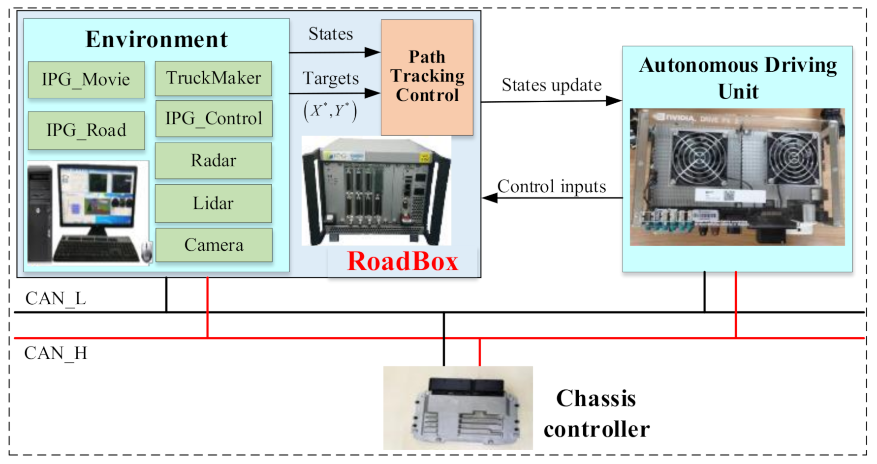
To ensure the effectiveness of the simulation, we built a hardware-in-the-loop simulation platform. The system framework of the hardware-in-the-loop simulation platform based on IPGXpack4, Chassis controller and Autonomous Driving Unit is shown in Figure 5. Among them, virtual test scenes, simulated vehicle models and sensor models are built and configured in TruckMaker and interact with peripherals (including radar, positioning and video signals) through IPGXpack4 (RoadBox). An autonomous Driving Unit is used to carry out the automatic driving tracking control. The acceleration/deceleration and steering control requirements are transmitted to the Chassis controller through the CAN protocol as the control output. Finally, the control demand outputs drive/brake and steering control commands through the Chassis controller and interacts with Xpack4 through CAN to realise the closed-loop control of the virtual actuator.

The basic parameters of the vehicle model are in

Table 2. The basic parameters of the vehicle model.

Parameters	Values	Parameters	Values
Traction coefficient	0.85	Front wheelbase	1.421 [m]
Front tire lateral stiffness	−1037 [N/deg]	Rear wheelbase	1.434 [m]
Rear tire lateral stiffness	−1105 [N/deg]	Equivalent torsional inertia	4600 [kg·m2]
Vehicle mass	2270 [kg]	Frontal area	2.8 [m2]
Gravity acceleration	9.8 [m/s2]	Coefficient of Drag	0.28

For the parameters configuration of the MPC controller, the reader can refer to [26,27].

.

4.2. Simulation Results

The reference path is generated for validation and evaluation according to the real GPS data. The target tracking speed is set to 60 km/h, and the constraints of yaw rate and the comfortable acceleration are set to 10 deg/s and 0.2 g, respectively.

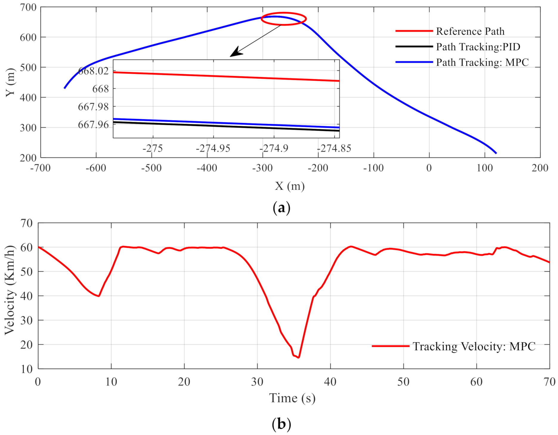
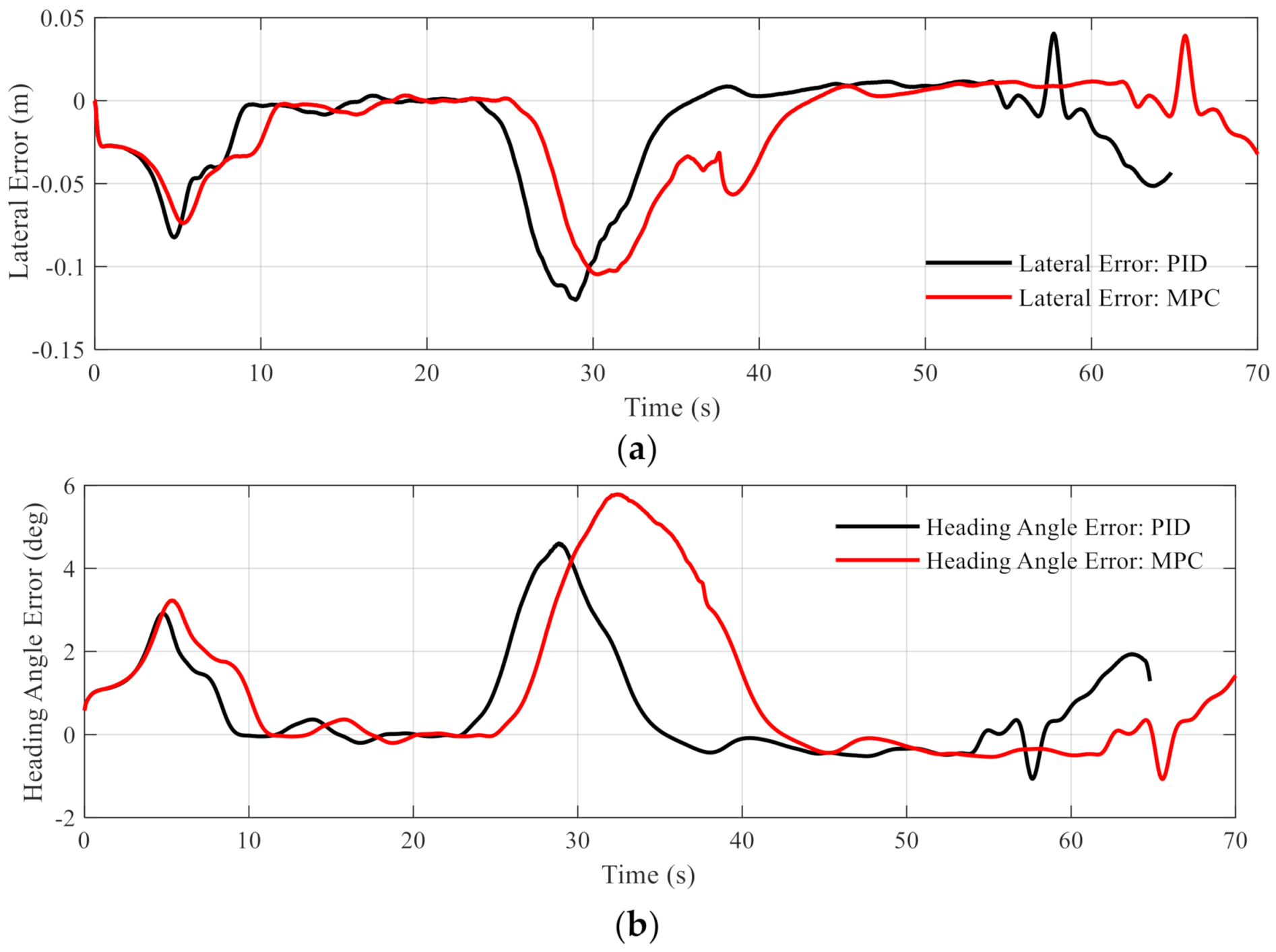
In the path tracking control with the target tracking speed set to 60 km/h, the reference trajectory results of the PID controller and the MPC controller are shown in Figure 6a,b, respectively. The lateral and heading errors are shown in Figure 7a,b, respectively. The simulation results show that, at a tracking speed of 60 km/h, both PID control and MPC control meet the requirements of lateral tracking accuracy. The two controllers’ lateral and heading errors are within 15 cm and 6 deg, respectively. Thus, compared with the lateral tracking of PID Control, the MPC exhibits better performance. The simulation result of tracking the target speed is shown in Figure 6b. Since a single PID controller can only achieve tracking control of a single target, the PID controller only carries closed-loop control based on the lateral position error feedback without interfering with the vehicle’s Longitudinal control. The longitudinal speed of the vehicle always maintains 60 km/h. The tracking control based on MPC controller involves multiple constraint processing and multiple target tracking. In constraint processing, the target speed as a soft constraint can deviate from a particular value at the expense of slack penalty terms to ensure better vehicle stability during path tracking. As shown in Figure 6b, at 28 s, when the vehicle is travelling close to a large curvature curve, if the vehicle is turned at a speed of 60 km/h, the stability and driving safety of the vehicle cannot be guaranteed. In the design of the MPC controller, the yaw rate and lateral acceleration are unbreakable hard constraints on vehicle dynamics. When optimising the objective function in the feasible region, the optimal objective function will be solved at the expense of speed tracking accuracy. When the curvature decreases (after the turn is completed), the longitudinal target speed of the vehicle will be tracked again under the premise of ensuring the accuracy of lateral tracking. Therefore, the tracking control based on MPC is a multi-target coordinated control of the vehicle.

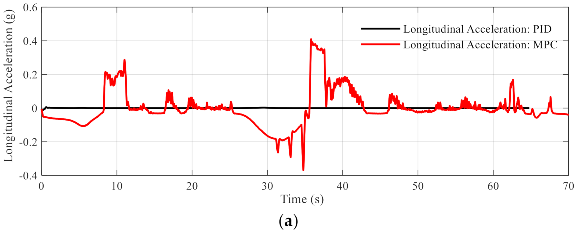
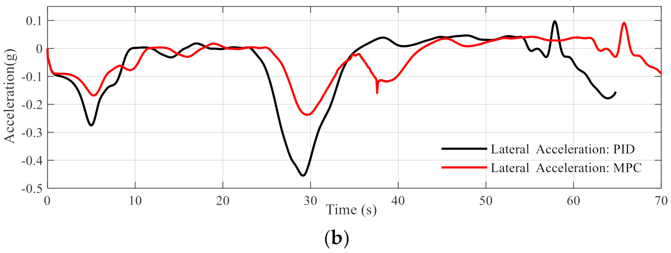
The comparison of the longitudinal and lateral acceleration during the path tracking of the autonomous vehicle is shown in Figure 8. As shown in Figure 8a, the longitudinal acceleration of the vehicle is always 0 in PID control, because only a single lateral tracking target is controlled in the path tracking. The lateral acceleration of PID control is shown by the black line in Figure 8b. The red line shows the longitudinal acceleration control based on the MPC in Figure 8a. To ensure that the vehicle can track stably, comfortably and safely, the path tracking of an autonomous vehicle under the MPC needs to combine the curvature of the reference trajectory and the vehicle stability constraints to control the longitudinal speed of the vehicle accordingly. Compared with the PID-based control, the average lateral acceleration of MPC drops from −0.0606 to −0.0376, the maximum acceleration fell from 0.4549 to 0.22 and the standard deviation decrease from 0.1194 to 0.0682.

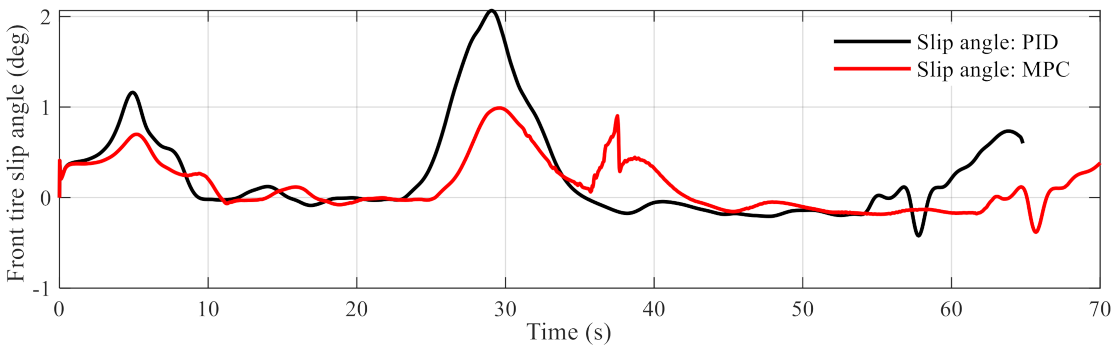
The comparison of yaw rate and front tire slip angle under PID and MPC tracking control are shown in Figure 9. Compared with MPC controller, PID controller with direct error feedback only carries out closed-loop control for a single target, which leads to a larger maximum and average front wheel slip angle. The maximum, average and standard deviation of the front wheel slip angle under PID control are 2.0653, 0.2494 and 0.5210, respectively. The maximum, average and standard deviation of the front wheel slip angle under MPC control are 0.9895, 0.1480 and 0.2921, respectively. The sideslip under PID control will expand as the curvature of the path to be tracked increases, eventually increasing the vehicle’s risk of sideslip and instability.

The single control step in the controller is distributed in 3–5 ms, which meets the demand of the control response.

5. Conclusions

To improve the measurement accuracy of the vehicle state in the tracking control, based on the extended Kalman filter theory, we integrated the vehicle GPS and IMU information and designed a vehicle state estimator with three inputs, six states and four outputs. To meet the requirements of multi-target tracking control in the longitudinal and lateral directions of autonomous vehicles, based on the 3DOF vehicle dynamics model and the curvilinear road coordinate system, we carried out dimensionality reduction on the longitudinal and lateral errors in the path tracking. To realise the online application of predictive control algorithm, based on the convex optimisation and the online active set theory with an open source QP solver, we designed and implemented a fast-rolling optimisation algorithm for longitudinal and lateral tracking control of autonomous vehicles and completed the verification of the algorithm and tracking performance in the reconstructed curve road scene based on real GPS data. The hardware-in-the-loop simulation results show that the proposed control can meet the tracking control need of autonomous driving. Compared with the PID-based controller, the proposed MPC controller has apparent advantages in lateral errors, lateral acceleration and front tire slip angle.

In the next step, we will further apply the proposed algorithm on other autonomous vehicles with specific driving environment. Moreover, the proposed strategy will be tested with a specific vehicle controller where the computing resources are limited. In this case, it is demanding to find a cost-efficient solver to trade off the optimization performance and the computing complexity.

References

- Anastasiadou, K.; Gavanas, N.; Pitsiava-Latinopoulou, M.; Bekiaris, E. Infrastructure Planning for Autonomous Electric Vehicles, Integrating Safety and Sustainability Aspects: A Multi-Criteria Analysis Approach. Energies 2021, 14, 5269. [Google Scholar] [CrossRef]
- Tostado-Véliz, M.; León-Japa, R.S.; Jurado, F. Optimal electrification of off-grid smart homes considering flexible demand and vehicle-to-home capabilities. Appl. Energy 2021, 298, 117184. [Google Scholar] [CrossRef]
- Hoffmann, G.M.; Tomlin, C.J.; Montemerlo, M.; Thrun, S. Autonomous Automobile Trajectory Tracking for Off Road Driving: Controller Design, Experimental Validation and Racing. In Proceedings of the 2007 American Control Conference, New York, NY, USA, 9–13 July 2007; pp. 2296–2301. [Google Scholar]
- Hayakawa, Y.; White, R.; Kimura, T.; Naito, G. Driver compatible steering system for wide speed range path following. IEEE/ASME Trans. Mechatron. 2004, 9, 544–552. [Google Scholar] [CrossRef]
- Netto, M.; Blosseville, J.; Lusetti, B.; Mammar, S. A new robust control system with optimized use of the lane detection data for vehicle full lateral control under strong curvatures. In Proceedings of the 2006 IEEE Intelligent Transportation Systems Conference, Toronto, ON, Canada, 17–20 September 2006; pp. 1382–1387. [Google Scholar]
- Zhang, W. The energy saving simulation of suspension robot path tracking based on improved PID control. Mach. Des. Manuf. Eng. 2019, 48, 29–32. [Google Scholar]
- Lee, H.; Tomizuka, M. Coordinated Longitudinal and Lateral Motion Control of Vehicles for IVHS. J. Dyn. Syst. 2001, 123, 535. [Google Scholar] [CrossRef]
- Brown, M.; Funke, J.; Erlien, S.; Gerdes, J.C. Safe driving envelopes for path tracking in autonomous vehicles ScienceDirect. Control Eng. Pract. 2017, 61, 307–316. [Google Scholar] [CrossRef]
- Kumarawadu, S.; Lee, T.T. Neuroadaptive Combined Lateral and Longitudinal Control of Highway Vehicles Using RBF Networks. IEEE Trans. Intell. Transp. Syst. 2006, 7, 500–512. [Google Scholar] [CrossRef]
- Zhao, X.; Chen, H. A Study on Lateral Control Method for the Path Tracking of Intelligent Vehicles. Automot. Eng. 2011, 33, 18–23. [Google Scholar]
- Hu, C.; Jing, H.; Wang, R.; Yan, F.; Chadli, M. Robust H∞ output-feedback control for path following of autonomous ground vehicles. Mech. Syst. Signal Process. 2015, 70, 414–427. [Google Scholar]
- Pan, S.; Changfu, Z.; Masayoshi, T. Combined Longitudinal and Lateral Control for Automated Lane Guidance of Full Drive by Wire Vehicles. SAE Int. J. Passeng. Cars Electron. Electr. Syst. 2015, 8, 477–485. [Google Scholar]
- Guo, H.; Cao, D.; Chen, H.; Sun, Z.; Hu, Y. Model predictive path following control for autonomous cars considering a measurable disturbance: Implementation, testing, and verification. Mech. Syst. Signal Process. 2019, 118, 41–60. [Google Scholar] [CrossRef]
- Du, X.; Htet, K.K.K.; Tan, K.K. Development of a Genetic-Algorithm-Based Nonlinear Model Predictive Control Scheme on Velocity and Steering of Autonomous Vehicles. IEEE Trans. Ind. Electron. 2016, 63, 6970–6977. [Google Scholar] [CrossRef]
- Li, S.E.; Jia, Z.; Li, K.; Cheng, B. Fast Online Computation of a Model Predictive Controller and Its Application to Fuel Economy–Oriented Adaptive Cruise Control. IEEE Trans. Intell. Transp. Syst. 2015, 16, 1199–1209. [Google Scholar] [CrossRef]
- Sun, J. Research on Tracking Control Algorithm of Unmanned Vehicle Based on Model Predictive Control (in Chinese). Master’s Thesis, Beijing Institute of Technology, Beijing, China, 2015. [Google Scholar]
- Wang, H. Research on Intelligent Vehicle Motion Control Based on Integrated Longitudinal and Lateral Control (in Chinese). Master’s Thesis, Nanjing University of Aeronautics and Astronautics, Nanjing, China, 2016. [Google Scholar]
- Zhang, L.; Wu, G.; Guo, X. Path Tracking Using Linear Time-varying Model Predictive Control for Autonomous Vehicle. J. Tongji Univ. Nat. Sci. 2016, 44, 1595–1603. [Google Scholar]
- Chen, S.; Chen, H.; Dan, N. Implementation of MPC-Based Path Tracking for Autonomous Vehicles Considering Three Vehicle Dynamics Models with Different Fidelities. Automot. Innov. 2020, 3, 386–399. [Google Scholar] [CrossRef]
- Zhao, N.N.; De-Min, X.U.; Gao, J.; Zhang, Q.N. Formation Path Following Control of Multiple AUVs Based on Serret-Frenet Coordinate System. Torpedo Technol. 2015, 23, 35–39. [Google Scholar]
- Ferreau, H.J.; Kirches, C.; Potschka, A.; Bock, H.G.; Diehl, M. QpOASES: A parametric active-set algorithm for quadratic programming. Math. Program. Comput. 2014, 6, 327–363. [Google Scholar] [CrossRef]
- Forsgren, A.; Gill, P.E.; Wong, E. Technical Report: Active-set methods for convex quadratic programming. Mathematics 2015. Available online: http://www.optimization-online.org/DB_FILE/2015/03/4848.pdf (accessed on 1 October 2021).
- Goldfarb, D.; Liu, S. An O(n3L) primal interior point algorithm for convex quadratic programming. Math. Program. 1990, 49, 325–340. [Google Scholar] [CrossRef]
- Axehill, D.; Hansson, A. A dual gradient projection quadratic programming algorithm tailored for model predictive control. In Proceedings of the IEEE Conference on Decision & Control, Cancun, Mexico, 9–11 December 2008. [Google Scholar]
- Arioli, M.; Baldini, L. A Backward Error Analysis of a Null Space Algorithm in Sparse Quadratic Programming. Siam J. Matrix Anal. Appl. 2002, 23, 425–442. [Google Scholar] [CrossRef]
- Lu, B.; Li, G.; Yu, H.; Wang, H.; Guo, J.; Cao, D.; He, H. Adaptive Potential Field Based Path Planning for Complex Autonomous Driving Scenarios. IEEE Access 2020, 8, 225294–225305. [Google Scholar] [CrossRef]
- Lu, B.; He, H.; Yu, H.; Wang, H.; Li, G.; Shi, M.; Cao, D. Hybrid Path Planning Combining Potential Field with Sigmoid Curve for Autonomous Driving. Sensors 2020, 20, 7197. [Google Scholar] [CrossRef] [PubMed]
Figure 1.
The 3DOF vehicle dynamics model.
Figure 2.
Geometric description of the reference road.
Figure 3.
Path generation based on the comprehensive road potential field.
Figure 4.
Lateral error description in Frenet coordinate system.
Figure 5.
Hardware-in-the-loop simulation platform.
Figure 6.
Path tracking results of two controllers, PID−based and MPC-based: (a) The path tracking of two controllers; (b)The tracking velocity based on MPC. Figure 7 The lateral errors and heading angle errors comparison of two controllers, PID and MPC: (a) The lateral errors of two controllers; (b) The heading angle errors of two controllers.
Figure 7.
The lateral errors and heading angle errors comparison of two controllers, PID and MPC: (a) The lateral errors of two controllers; (b) The heading angle errors of two controllers.
Figure 8.
Acceleration comparison of two controllers, PID and MPC: (a) Longitudinal acceleration of two controllers; (b)Lateral acceleration of two controllers.
Figure 9.
Front tire slip angle comparison of PID and MPC controller.