Influence of Structural Stiffness and Loss Factor on Railroad Vehicle Comfort

Abstract

This paper presents a new formulation for analyzing a beam on elastic supports traveling on irregular profiles. The model is a first approximation of a passenger railway vehicle car body. The main difference with previous works is the use of a complex modulus to represent structural damping rather than relying on equivalent viscous terms. The formulation groups rigid body modes with flexible modes and proposes a matrix form that is easy to interpret and solve in the frequency domain. Comfort indexes are readily obtained from weighted response spectral densities. The model is used to assess the influence of structural damping and stiffness on comfort. It will be shown that the evolution of comfort with stiffness is non-monotonic and, therefore, comfort does not always improve as stiffness increases.

1. Introduction

There are two current trends in passenger rail transport that may influence comfort in a negative way. One of these trends is the increase in operational speeds on new and existing high-speed train tracks. The other is weight reduction when achieved at the cost of structural stiffness. The influence of the structural response on comfort is acknowledged by most rolling stock manufacturers, who routinely take it into account in their simulations. Multibody (MB) analyses conducted to predict dynamic behavior and comfort often include flexible frames represented by mass, damping, and stiffness matrices (or condensed versions of these matrices) derived from finite element models (FEM). These combined MB–FEM analyses show the influence of many design features on comfort but, at the same time, often hide the basic relationships between the most fundamental design parameters and passenger vibration. To unveil these relationships, it is helpful to strip the models down to their bear minimum. For instance, despite the fact that connected cars influence the vertical dynamics of one another, the inclusion of all cars in the models may obscure the basic connection between comfort and structural stiffness. Most simplified studies, such as the one presented in this paper, consider a single isolated car on two trucks or bogies [1,2,3,4,5,6,7,8,9]. Our case, however, differs in that it focuses on vehicles in which consecutive cars share either a bogie or a yoke with independent wheels (such as the configurations patented by the Spanish manufacturer “Talgo”). In either case, the cars are supported at the very end of their structure, as shown by the models described in the next section. The second simplifying step is to disregard the mechanical complexities of the suspension, ignore unsuspended and semi-suspended masses, and represent the system as a simple linear spring–damper set. The third and bolder simplification is to assume that the car structure behaves like a uniform cross-section Euler–Bernoulli beam with all mass (including payload) evenly distributed along the beam.

Similar models have been analyzed in a number of papers [1,2,3,4,5,6,7,8,9] with the same goal that drives our research: to assess the influence of structural flexibility on passenger comfort. However, to the best of our knowledge, no previous work on this particular subject has modeled structural dissipation by means of a complex modulus. They all include a viscous term in the equation of motion of the beam that stems from cross-section stresses proportional to strain rate and in-phase with strain rate. This Kelvin–Voigt damping, also referred to as strain-rate damping, is convenient because it complies with the principle of causality, allowing models to be analyzed in the time domain.

Zhou et al. [1] analyzed a Euler–Bernoulli beam with strain-rate damping supported on two bogies. They quantified comfort via the Sperling index and concluded that comfort improves with stiffer beams. They also showed that to maintain comfort levels for higher speeds, structures should be made stiffer. Huang et al. [2], as well as Shi et al. [3], used the same model with a mass under the beam connected with a flexible element to represent the effect of undercarriage equipment. They showed that the equipment could be used as a dynamic vibration absorber when the connecting stiffness and damping characteristics are properly designed. They compared their model results to experimental measurements, which showed good agreement. Gong et al. [4] also used the same basic model but fitted, in this case, with underframe dampers. They showed that properly placed dampers could mitigate the flexural vibration of the car frame. Their model results were compared to finite element results, showing good agreement.

Dumitriu [5,6,7,8,9] has conducted similar studies also using a Euler–Bernoulli beam with strain-rate damping supported on two bogies. She first presents the model as a viable tool for virtual certification [5] and later [6] uses the model to show that the consideration of frame flexibility may shift the least comfortable point on the beam from atop the bogie (for a rigid beam) to the beam center (for a flexible beam under particular conditions).

The ubiquity of the strain-rate damping model notwithstanding, its ability to represent structural damping is questionable. The energy dissipated per cycle grows with frequency in the case of viscous damping, whereas experience shows otherwise. Banks and Inman [10] conducted experimental tests with composite beams, from which the damping parameters of several models they proposed were extracted. The analytical time response obtained with the estimated coefficients was then compared to the experimentally measured time response. Their hysteresis models produced better results than the strain-rate damping model. Dropping the Kelvin–Voigt term in favor of a complex modulus for the beam material is a better option to represent structural damping. In this case, damping stresses are proportional to strain (rather than strain rate), albeit in-phase with the strain rate. The drawback of complex modulus is that the principle of causality is lost, and models are not amenable to time-domain analysis. Fortunately, frequency domain analysis with a complex modulus is not only feasible but quite simple and straightforward as will be shown next. Moreover, mean square accelerations, from which comfort indexes may be estimated, can be easily obtained from frequency analyses.

2. Formulation

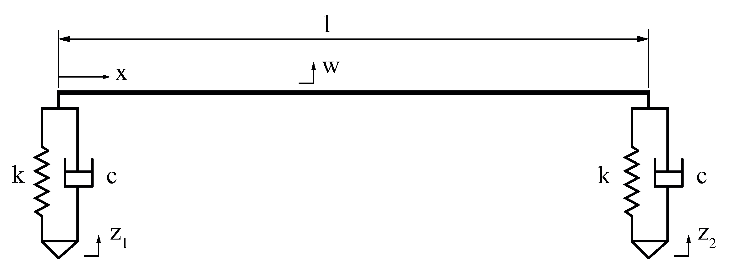
The model in Figure 1 is a uniform Euler–Bernoulli beam on two spring–damper sets. Let l be the length of the beam (equal, in our case, to the distance between axles, as mentioned in the introduction); I, its cross section area moment of inertia; m, its uniformly distributed mass (with $\mu =m/l$, the mass per unit length); $E_r$, the material storage modulus; and $\eta$, its loss factor (so that $E=E_r(1+i\eta )$). The suspension is simplified as linear springs and dampers at each end of the beam with no unsprung mass considered. As shown in Figure 1, k and c are the suspension stiffness and damping constants, respectively; $z_1$ and $z_2$, the front and rear wheel vertical displacements, respectively; x, the coordinate along the beam measured from the front axle; and $w(x,t)$, the vertical displacement of the beam. The equation of motion is

$$EI{w}^{IV}+\mu \ddot{w}=f$$

(1)

where Roman numerals indicate derivation with respect to x and dots derivation with respect to time. The right-hand side f ($f(x,t)$, that is) is the load distribution on the beam (gravitational forces not included since displacements are measured from the static equilibrium position). In our case, f is concentrated at each end of the beam and corresponds to the spring and damper forces that can be written as

$$f=\left(k\left(z_1-w_0\right)+c\left({\dot{z}}_1-{\dot{w}}_0\right)\right)\delta \left(0\right)+\left(k\left(z_2-w_l\right)+c\left({\dot{z}}_2-{\dot{w}}_l\right)\right)\delta \left(l\right)$$

(2)

where $w_0=w(0,t)$, $w_l=w(l,t)$, and $\delta$ is Dirac’s delta.

Displacements are expressed as the following superposition of n modes:

$$w(x,t)=\sum _{i=1}^n{W}_i\left(x\right)q_i\left(t\right)$$

(3)

where

$$\begin{array}{ccc}{W}_1\left(x\right)\hfill & =\hfill & 1\hfill \\ W_2\left(x\right)\hfill & =\hfill & x-l/2\hfill \\ W_i\left(x\right)\hfill & =\hfill & cos{\beta }_{i}x+cosh{\beta }_{i}x-\frac{cos{\beta }_{i}l-cosh{\beta }_{i}l}{sin{\beta }_{i}l-sinh{\beta }_{i}l}\left(sin{\beta }_{i}x+sinh{\beta }_{i}x\right)i\ge 3\hfill \end{array}$$

(4)

The first two functions being the rigid body modes, while the rest are flexible modes for the free–free boundary conditions, with ${\beta }_{i}l\approx (2i-3)\pi /2$ for $i\ge 3$. In principle, the set of modes for the case of a simply supported beam could also be used. Nevertheless, in that case, all resulting equations except for the two involving rigid body modes become homogeneous, and, therefore, amplitudes obtained from those equations could be arbitrarily scaled. Introducing Expressions (2) and (3) in Equation (1), multiplying by mode $W_i$, integrating along the length of the beam, and verifying that all modes (including rigid body modes) are orthogonal, the following equation is obtained:

$$\begin{array}{ccc}\hfill & \hfill & EI{\beta }_i^4\frac{m_i}{\mu }{q}_i+m_i{\ddot{q}}_i=\hfill \\ \hfill & \hfill & \left(k\left(z_1-w_0\right)+c\left({\dot{z}}_1-{\dot{w}}_0\right)\right)W_i\left(0\right)+\left(k\left(z_2-w_l\right)+c\left({\dot{z}}_2-{\dot{w}}_l\right)\right)W_i\left(l\right)\hfill \end{array}$$

(5)

where mode $W_i$ could be any of the n modes included (making Equation (5), in fact, a system of n ordinary differential equations), and where $m_i=m$ for $i=1,3,\dots n$, and $m_2=I_g$, the rigid beam moment of inertia with respect to its center of mass. Using Equation (3) to express displacements and velocities at each end of the beam ($w_0$, ${\dot{w}}_0$, $w_l$, and ${\dot{w}}_l$) as a superposition of modes, the set of equations can be written as

$$\begin{array}{ccc}\hfill & \hfill & EI{\beta }_i^4\frac{m_i}{\mu }{q}_i+m_i{\ddot{q}}_i=\left(k{z}_1+c{\dot{z}}_1\right)W_i\left(0\right)+\left(k{z}_2+c{\dot{z}}_2\right)W_i\left(l\right)-\hfill \\ \hfill & \hfill & k\sum _{j=1}^n\left(W_j\left(0\right)W_i\left(0\right)+W_j\left(l\right)W_i\left(l\right)\right)q_j-c\sum _{j=1}^n\left(W_j\left(0\right)W_i\left(0\right)+W_j\left(l\right)W_i\left(l\right)\right){\dot{q}}_{j}i=1,\dots n\hfill \end{array}$$

(6)

Defining vectors $\mathbf{q}$, $\mathbf{W}$, ${\mathbf{W}}_0$, and ${\mathbf{W}}_l$ as

$$\mathbf{q}=\left\{\begin{array}{c}{q}_1\\ ⋮\\ q_n\end{array}\right\}\mathbf{W}=\left\{\begin{array}{c}{W}_1\left(x\right)\\ ⋮\\ W_n\left(x\right)\end{array}\right\}{\mathbf{W}}_0=\left\{\begin{array}{c}{W}_1\left(0\right)\\ ⋮\\ W_n\left(0\right)\end{array}\right\}{\mathbf{W}}_l=\left\{\begin{array}{c}{W}_1\left(l\right)\\ ⋮\\ W_n\left(l\right)\end{array}\right\}$$

(7)

matrices $\mathbf{M}$ and $\mathbf{B}$ as

$$\mathbf{M}=\left[\begin{array}{ccccc}m& & & & \\ & I_g& & & \\ & & m& & \\ & & & \ddots & \\ & & & & m\end{array}\right]\mathbf{B}=\left[\begin{array}{ccccc}0& & & & \\ & 0& & & \\ & & {\beta }_3^4& & \\ & & & \ddots & \\ & & & & {\beta }_n^4\end{array}\right]$$

(8)

and matrix $\mathbf{A}$ as ${\mathbf{W}}_0{\mathbf{W}}_0^T+{\mathbf{W}}_l{\mathbf{W}}_l^T$, Equations (6) can be grouped in matrix form as

$$\mathbf{M}\ddot{\mathbf{q}}+c\mathbf{A}\dot{\mathbf{q}}+\left(k\mathbf{A}+\frac{EI}{\mu }\mathbf{B}\mathbf{M}\right)\mathbf{q}=\left(k{z}_1+c{\dot{z}}_1\right){\mathbf{W}}_0+\left(k{z}_2+c{\dot{z}}_2\right){\mathbf{W}}_l$$

(9)

It is worth noting that this system of equations reduces to the dynamic equations of a rigid body on two elastic supports when all modes are discarded except for the first two.

For harmonic input, $z_1=Z{e}^{i\omega t}$, harmonic solutions of Equation (9) may be sought in the form $\mathbf{q}=\mathbf{Q}{e}^{i\omega t}$, in which case Equation (9) becomes the following set of algebraic equations:

$$\left[k\mathbf{A}+i\omega c\mathbf{A}+\frac{EI}{\mu }\mathbf{B}\mathbf{M}-{\omega }^2\mathbf{M}\right]\mathbf{Q}=Z(k+i\omega c)\left({\mathbf{W}}_0+e^{-i\omega l/v}{\mathbf{W}}_l\right)$$

(10)

where input $z_2$ lags behind $z_1$ the time it takes the vehicle to travel the distance l, that is $z_2=Z{e}^{i\omega (t-l/v)}$, with v, the vehicle speed. Given the Fourier transform Z of input $z_1$, vector $\mathbf{Q}$ can be obtained by solving Equation (10) for each frequency $\omega$. Each component of vector $\mathbf{Q}$ represents the amplitude with which the corresponding mode participates in beam motion at frequency $\omega$. Nevertheless, it will soon be clear that, for the purpose of comfort assessment, it is more convenient to solve Equation (10) for the quotient $\mathbf{Q}/Z$, in which case Fourier transform Z need not be explicitly specified. This fraction, which will be referred to as ${\mathbf{H}}_1$ in what follows, can be interpreted as a vector of transfer functions between input $z_1$ and “modal” time responses $\mathbf{q}$. Using the vectors defined in Equation (7), the summation in Equation (3) can be written as

$$w={\mathbf{W}}^T\mathbf{q}$$

(11)

For the harmonic case ($\mathbf{q}=\mathbf{Q}{e}^{i\omega t}$), defining W (not to be mistaken with vector $\mathbf{W}$ nor its components $W_i$) such that $w=W{e}^{i\omega t}$, the following relations hold:

$$w=W{e}^{i\omega t}={\mathbf{W}}^T\mathbf{q}={\mathbf{W}}^T\mathbf{Q}{e}^{i\omega t}={\mathbf{W}}^T{\mathbf{H}}_{1}Z{e}^{i\omega t}={\mathbf{W}}^T{\mathbf{H}}_1{z}_1$$

(12)

Therefore, the transfer function defined as $H_2=W/Z$ can be computed as

$$H_2={\mathbf{W}}^T{\mathbf{H}}_1$$

(13)

This transfer function can now be used to determine the response spectral density in terms of the input spectral density. However, comfort indexes are determined from a filtered or weighted response rather than from the raw signal. The goal is to take into account the effect of the different frequencies on comfort. For a detailed explanation of the calculation procedure, as well as of the meaning, of the comfort index used in this work, see [11]. Filtering in the time domain is tantamount to multiplying by the filter transfer function in the frequency domain. Therefore, multiplying $H_2$ by the comfort filter (let it be referred to as $H_c$) yields the transfer function between weighted accelerations (${\ddot{w}}_w$) and input acceleration (${\ddot{z}}_1$) as $H=H_2{H}_c$. The spectral density of the weighted response can thus be obtained as

$$S_{{\ddot{w}}_w}={\left|H\right|}^2{S}_{{\ddot{z}}_1}={\left|H\right|}^2{\omega }^4{S}_{z_1}\left(\omega \right)={\left|H\right|}^2{\omega }^4{S}_{z_1}(\Omega )/v$$

(14)

where the input spectral density $S_{z_1}$ is usually expressed in terms of spatial frequency $\Omega$ (with $\Omega =\omega /v$, in rad/m). In fact, reference [12] suggests that $S_{z_1}(\Omega )$ may be assumed to be given by

$$S_{z_1}=\frac{A_v{\Omega }_c^2}{({\Omega }^2+{\Omega }_r^2)({\Omega }^2+{\Omega }_c^2)}$$

(15)

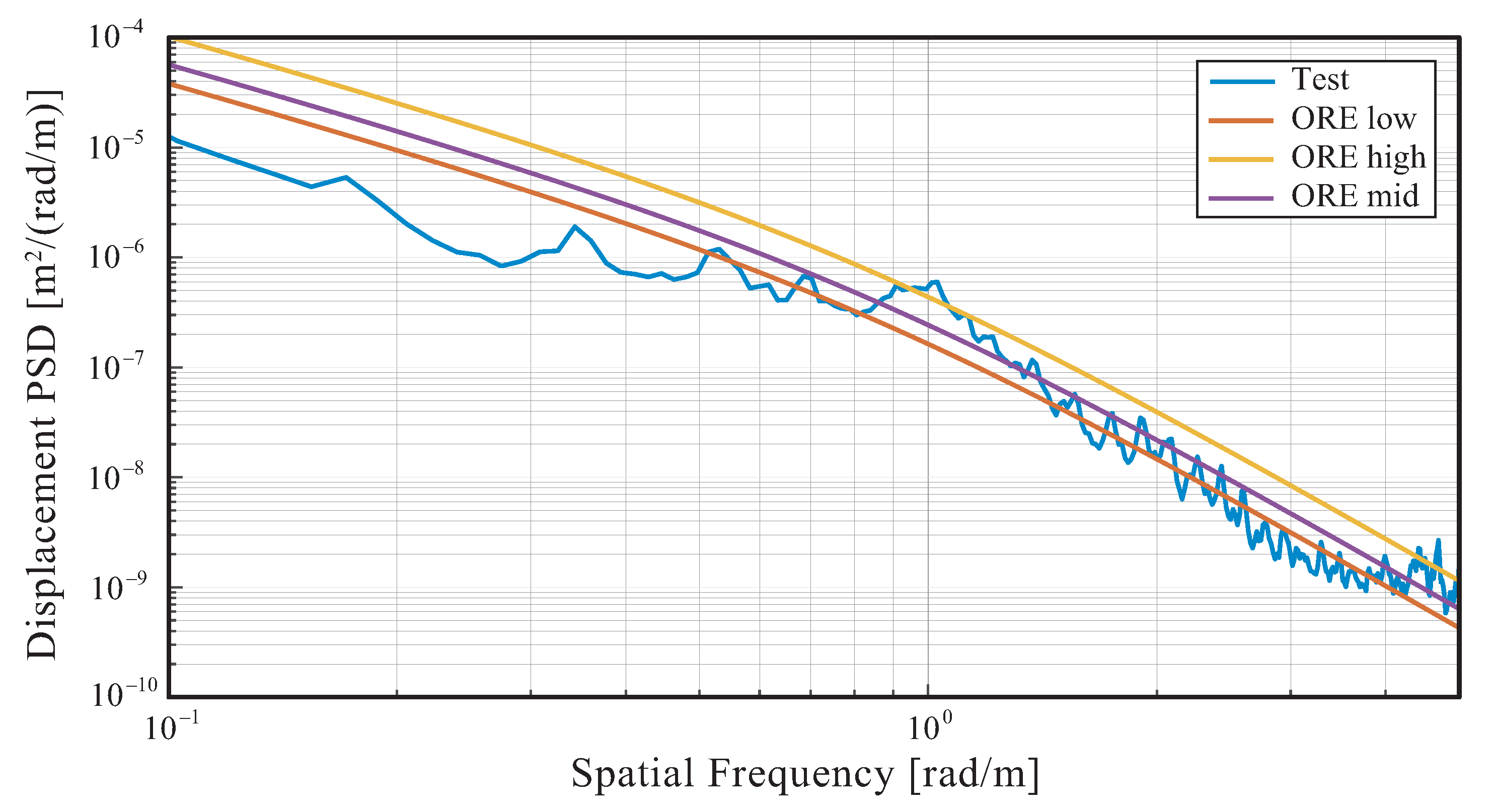
where ${\Omega }_c=0.8246$ rad/m, ${\Omega }_r=0.0206$ rad/m, and parameter $A_v$ can be fine-tuned to represent different track irregularity levels. Figure 2 plots Expression (15) for the following values of $A_v$: $A_v=0.4032$$\mathsf{ \mu }$m rad, which is considered a low irregularity track (labelled “ORE low” in the Figure), $A_v=1.08$$\mathsf{ \mu }$m rad, which is considered high irregularity (labelled “ORE high” in the Figure), and $A_v=0.6$$\mathsf{ \mu }$m rad as an intermediate value (labelled “ORE mid” in the Figure). The figure also plots an instance of experimental measurements conducted by the authors in collaboration with the Spanish rolling stock manufacturer “Talgo” on board their test train “Avril”. The experimental spectral density is computed from accelerations measured on one of the journal boxes when the train was traveling at 300 km/h on a high-speed train track. It can be seen that Expression (15) cannot be a perfect interpolating function for all tracks and stretches, and that, at least in this instance, some frequency bands are better captured by the expression than others. Experimental deviations notwithstanding, our test data allow us to state that Expression (15), with the appropriate $A_v$ value, and adjusting parameters ${\Omega }_r$ and ${\Omega }_c$ if needed, can be a fair representation of the frequency content of many tracks.

Integrating $S_{{\ddot{w}}_w}$ of Equation (14) into the range of relevant frequencies yields the mean squared weighted acceleration ($E\left[{\ddot{w}}_w^2\right]$), from which comfort indexes are readily calculated (see [11]) as $c_I=6\sqrt{E\left[{\ddot{w}}_w^2\right]}$ (note that this definition makes the index decrease as comfort improves). The comfort filter $H_c$ strongly attenuates frequencies above 30 Hz. The contribution of higher frequencies to comfort indexes may thus be neglected.

The proposed procedure formulated in this section is extremely efficient in terms of computational cost. The dimension of the system of linear algebraic equations to be solved (Equation (10)) is small since just a few modes suffice to represent structural flexibility. It is true, nonetheless, that the system needs to be solved for every frequency in the range of interest and that the resulting spectral density needs to be integrated, but neither of these tasks is a big burden on the computational cost.

3. Complex Modulus versus Viscous Damping for Comfort Assessment

As stated in the introduction, there are solid theoretical arguments, as well as some experimental evidence, in favor of complex moduli as opposed to viscous terms to model structural damping. Nevertheless, it was also mentioned that, despite the loss in accuracy, most researchers resort to viscous terms. To quantify the difference, the formulation in the previous section can easily be tweaked to include viscous damping. The equivalent of Equation (1) is now

$$E_{r}I{w}^{IV}+\nu I{\dot{w}}^{IV}+\mu \ddot{w}=f$$

(16)

where $\nu$ is the viscous modulus that, forcing the imaginary parts of Equations (1) and (16) to coincide at the first bending frequency, is given by

$$\nu =\frac{\eta }{{(\pi /l)}^2}\sqrt{\frac{E_r\mu }{I}}$$

(17)

Using the same procedure and notation as in the previous section, the equivalent of Equation (10) is now

$$\left[k\mathbf{A}+i\omega c\mathbf{A}+\frac{E_{r}I}{\mu }\mathbf{B}\mathbf{M}+i\omega \nu Il\mathbf{B}-{\omega }^2\mathbf{M}\right]\mathbf{Q}=Z(k+i\omega c)\left({\mathbf{W}}_0+e^{-i\omega l/v}{\mathbf{W}}_l\right)$$

(18)

The same frequency analysis described above can be used to quantify comfort indexes at any location along the beam for any given set of parameters. For instance, let all parameters take the values shown in the first row of

Table 1. Parameters used to obtain each of the figures.

Fig.	${\mathit{A}}_{\mathit{v}}$ ($\mathsf{\mu }$m rad)	l (m)	m (kg)	${\mathit{f}}_{\mathit{b}}$ (Hz)	${\mathit{\xi }}_{\mathit{b}}$	${\mathit{E}}_{\mathit{r}}$ (GPa)	$\mathit{\eta }$	${\mathit{f}}_3$ (Hz)	v (km/h)
Figure 3	0.6	13	13,370	1.3	0.05	70	0.01–0.1	8	300
Figure 4	-	13	-	∞	-	∞	-	∞	300
Figure 5	0.6	13	13,370	0.5–2	0.05	∞	-	∞	300
Figure 6	0.6	13	13,370	1.3	0.01–0.1	∞	-	∞	300
Figure 7 and Figure 8	0.6	13	13,370	1.3	0.05	70	0.01	6–20	300
Figure 9	0.6	13	13,370	1.3	0.05	70	0.01	6–40	300
Figure 10 and Figure 11	0.6	13	13,370	1.3	0.05	70	0.01–0.1	8	300
Figure 12	0.6	13	13,370	1.3	0.05	70	0.01–0.9	8	300
Figure 13 and Figure 14	0.6	13	13,370	1.3	0.05	70	0.01	8	90–360
Figure 15	0.6	13	13,370	1.3	0.05	70	0.01	8	90–500

. The loss factor can take values between 0.01 and 0.1. Figure 3 shows the evolution of the comfort index with a loss factor at two locations on the beam when computed using viscous damping (v.d. in the figure) as well as when using complex modulus (c.m.). It can be seen that differences between both damping models are quite significant when measured in terms of the comfort index. The viscous model greatly overestimates damping as the frequency increases, thus yielding too optimistic comfort index values, as Figure 3 attests. This result sheds some doubt on previous works and prompts experimental verification. This, however, lies beyond the scope this paper.

4. Application to Oversimplified Cases

Before using the formulation presented in the previous section to assess the influence of structural damping and flexibility on comfort, it is clarifying to use it for two oversimplified cases. The intention here is to present the order of magnitude of the comfort indexes for the values of the parameters to be used throughout this research and to show the shape of the comfort curves (i.e., comfort as a function of position along the beam) to help interpret the results of the next section. The two oversimplified cases are a rigid beam on stiff supports and a rigid beam on a suspension.

4.1. Rigid Beam on Stiff Supports. Geometric Filtering

The very well known phenomenon of geometric filtering is simply a consequence of the fact that all points on a stiff beam are located at intermediate heights between the front and the rear. If the front rises while the rear sinks (or vice versa), all points in between have smaller amplitudes. In fact, when the wavelength of a harmonic input is such that the front is on a crest while the rear is on a trough, the center of the beam does not move vertically. In that case, the amplitude of the vertical motion grows from zero at the center to the maximum at both ends.

While the previous paragraph is trivial, it is worth pointing out that many of these “filtered frequencies” for typical railway vehicle passenger car lengths and speeds lie within the range of interest for comfort evaluation. Input harmonics with frequencies $f=(n+0.5)v/l$, $n=0,1\dots$ are not felt at the center of a rigid beam on stiff supports. Higher speeds and shorter cars push some of these frequencies outside the 0–30 Hz range of interest, but even for the short cars built by the Spanish manufacturer “Talgo” (approximately 13 m), at 300 km/h, there are five filtered frequencies within said range.

Figure 4 shows the modulus of transfer function $H_2$ (Equation (13)) at four locations along a thirteen meter long rigid beam on infinitely stiff supports traveling at 300 km/h (see Table 1). Both ends of the beam are forced to replicate the input (stiff supports, $|H_2(0,f)|=|H_2(l,f)|=1$), whereas the amplitudes are attenuated elsewhere for most frequencies. Total canceling can only happen at the midpoint on the beam for the specific frequencies mentioned in the previous paragraph.

4.2. Rigid Beam. Influence of Suspension Parameters on Comfort

Although, as will be shown in the next section, structural behavior strongly influences comfort on a railway vehicle passenger car, it can nonetheless be confidently said that the suspension is the single most important system for comfort. To support this statement, comfort indexes will be determined using the formulation in Section 2 for a rigid car (removing flexible modes or setting a very large cross-section area moment of inertia I since both methods yield the same results) traveling at 300 km/h on an intermediate quality railroad ($A_v=0.6\mathsf{ \mu }$m rad in Equation (15)). The distance between axles is 13 m, the mass of the car is 13,370 kg, and the suspension damping factor is 5% (${\xi }_b=0.05$, with which $c={\xi }_b\sqrt{2 \mathrm{km}}$). Suspension stiffness will be specified in terms of bounce frequency ($f_b=\sqrt{2 \mathrm{k}/\mathrm{m}}/\left(2\pi \right)$) and allowed to vary from $f_b=0.5$ Hz to $f_b=2$ Hz (see Table 1).

Figure 5 shows comfort indexes at four locations along the beam versus the bounce frequency $f_b$. The plot clearly shows that comfort improves significantly as the suspension stiffness is reduced. Extremely soft suspensions ($f_b=0.5$ Hz) are so comfortable ($c_I<0.5$) that the added benefit of geometrical filtering towards the midpoint of the beam is hardly noticeable. On the other end of the range considered ($f_b=2$ Hz), the ride is very uncomfortable near the axles ($c_I>8$), but the effect of geometrical filtering is significant. Typical bounce frequencies for passenger railway vehicle secondary suspensions are in the vicinity of 1 Hz, which means that, on a track with $A_v=0.6\mathsf{ \mu }$m rad, at 300 km/h with ${\xi }_b=0.05$, not every location on the beam can be in the “very comfortable” range ($c_I<1.5$, see [11]), not to mention the case of poorer quality tracks.

The influence of suspension damping is depicted in Figure 6. Here again $l=13$ m, $v=300$ km/h, $A_v=0.6\mathsf{ \mu }$m rad, m = 13,370 kg, flexible modes have been removed, and suspension stiffness is now fixed at $f_b=1.3$ Hz, whereas the suspension damping factor ${\xi }_b$ is allowed to vary from 1 to 10% (see Table 1). Comfort improvements when going from undamped to a damping factor of a few percentage points are quite significant. Nevertheless, marginal benefits go down as ${\xi }_b$ grows; therefore, there is no point in increasing ${\xi }_b$ beyond moderate values (6 or 7%, for example).

5. Results

The formulation in Section 2 allows flexible modes to be included. To assess the influence of structural stiffness, the beam cross-section area moment of inertia (I) will be allowed to vary within a range that will be specified in terms of the first bending frequency of the free–free beam. To be consistent with the numbering of modes in Equation (4), the first bending frequency is tagged $f_3$. The relation between $f_3$ and I is

$$I=\frac{{\left(f_{3}2\pi \right)}^{2}m/l}{{(E_r{\beta }_3/l)}^4}$$

(19)

where $f_3$ is varied in the range from 6 Hz to 20 Hz, where the beam has been assumed to be made of aluminum, and thus $E_r=70{10}^9$ N/m${}^2$, and where ${\beta }_3\approx 4.13/l$. The rest of the parameters take the same values as in the previous section ($l=13$ m, $v=300$ km/h, $A_v=0.6\mathsf{ \mu }$m rad, $m=$ 13,370 kg, and $f_b=1.3$ Hz), with ${\xi }_b$ now fixed at ${\xi }_b=0.05$. The material loss factor ($\eta$) has been set at a higher value ($\eta =0.01$) than that of aluminum to better account for typical structural damping (see Table 1).

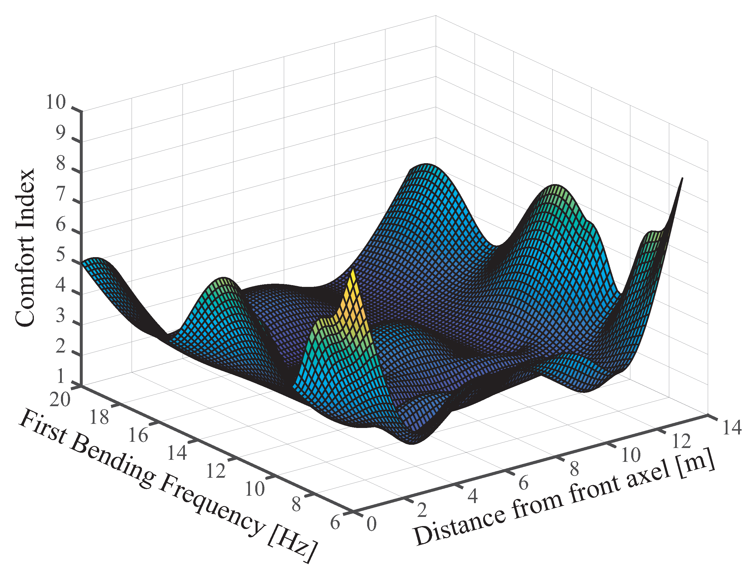
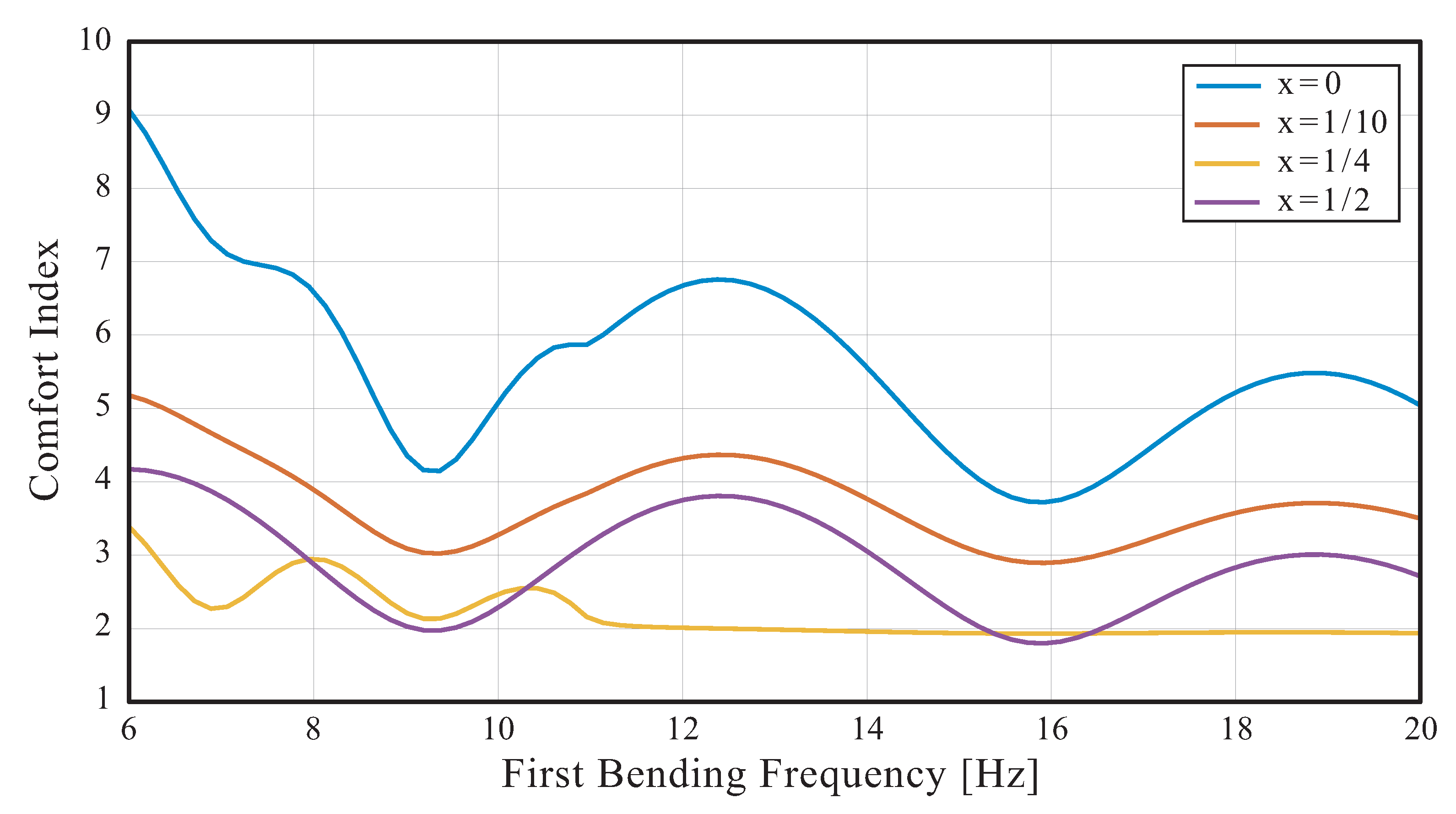
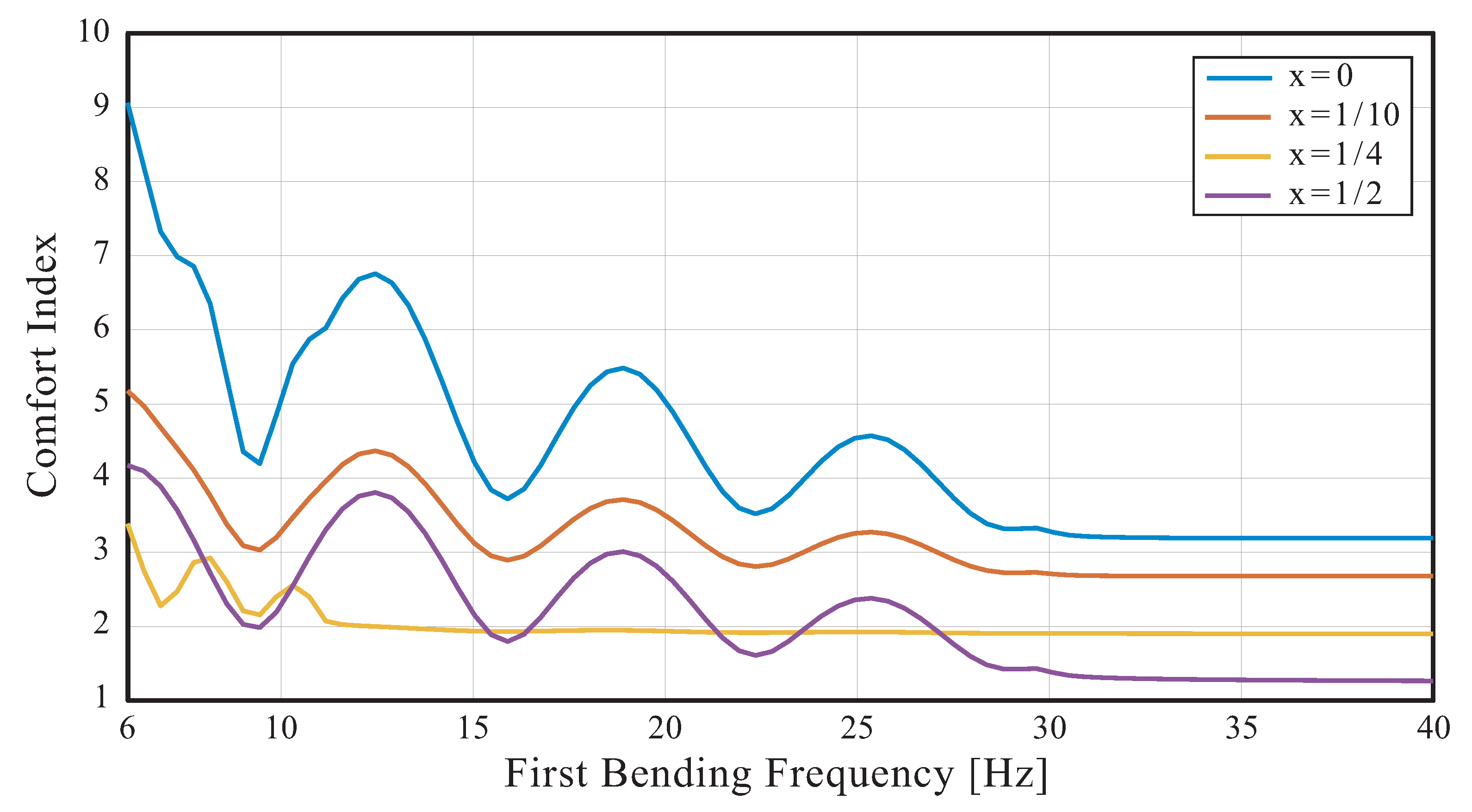
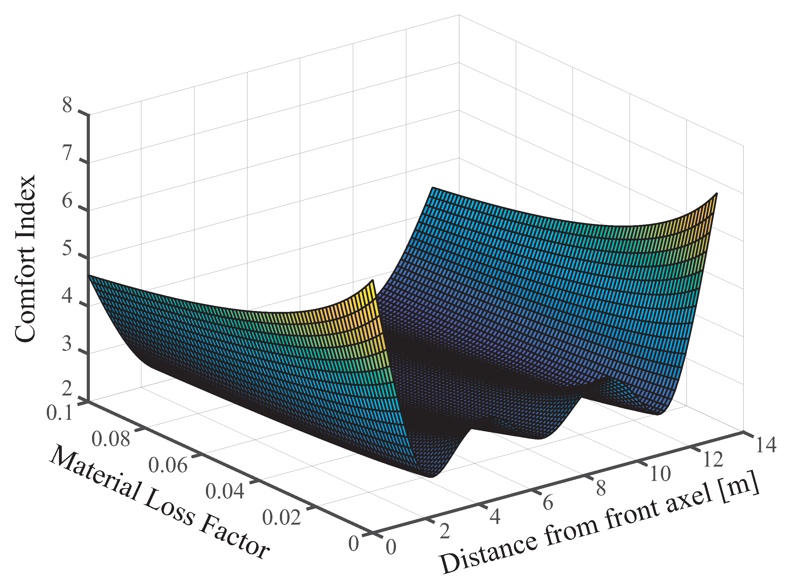
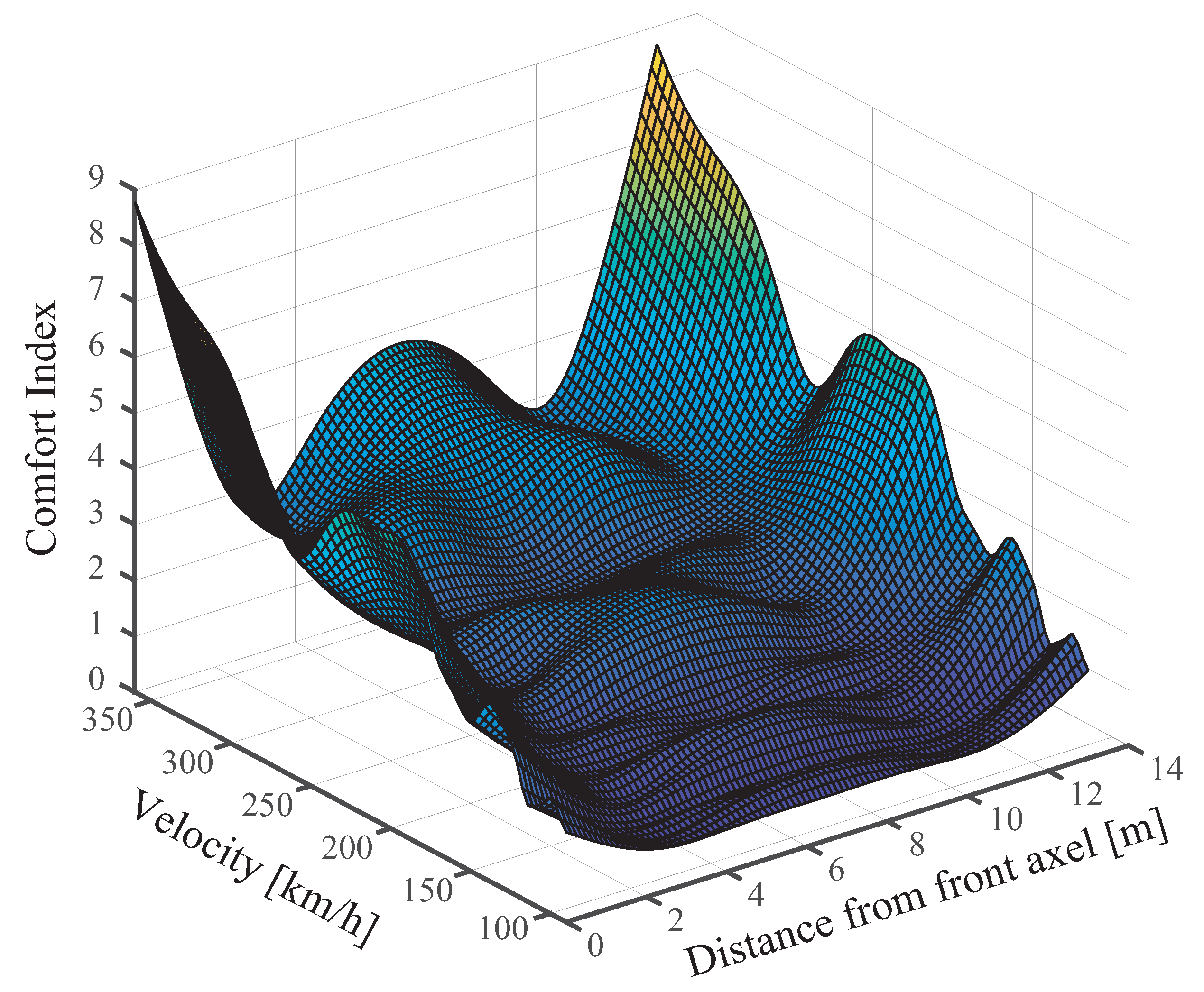
Figure 7 shows comfort indexes along the length of the beam versus bending frequency $f_3$, whereas Figure 8 shows sections of this surface at four locations along the beam. It could be said that, as a general trend, comfort improves as the structure stiffens. Nevertheless, the statement cannot be taken for granted since the dependence of the comfort index on stiffness is non-monotonic, thus proving the statement wrong every time the slope is positive in the $c_I$ vs. $f_3$ curve. This behavior makes the task of the designer particularly difficult. For example, stiffening the structure of the example under discussion beyond 9.3 Hz ($f_3>9.3$ Hz, Figure 8) worsens comfort at a great rate (measured as the slope of $c_I$ vs. $f_3$ for a given x). In fact, comfort does not start to improve again until $f_3$ reaches a value of approximately 15 Hz, and the improvement only happens for a short range of bending frequencies, starting to worsen again before $f_3$ reaches 16 Hz.

Despite the wavy evolution of comfort with stiffness, it is true that the values of the curves in Figure 8 lie above the corresponding values for the infinitely stiff beam analyzed in the previous section. This statement is supported by Figure 9 where the upper limit for the first bending frequency has been stretched beyond what is reasonable or even feasible (see Table 1). It can be seen that the non-monotonic comfort curves tend toward their corresponding rigid body asymptotes. These asymptotic values may be checked against those in Figure 5 for $f_b=1.3$ Hz or against those in Figure 6 for ${\xi }_b=0.05$.

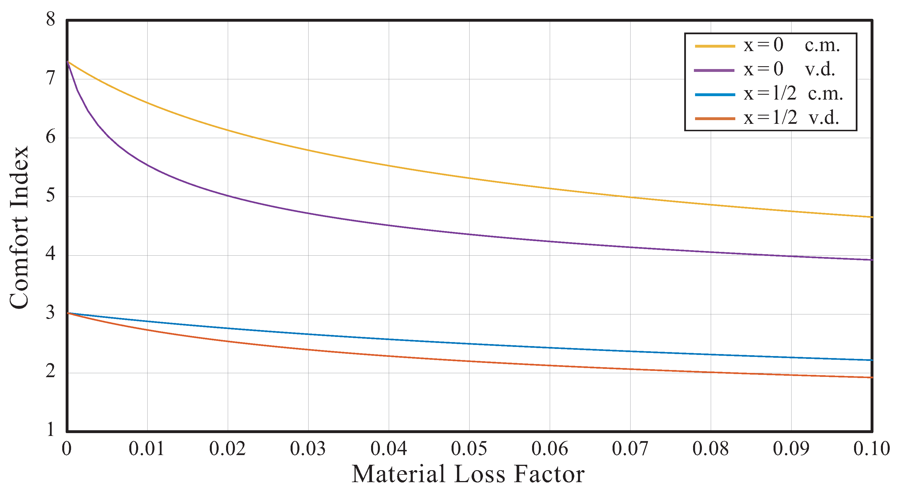
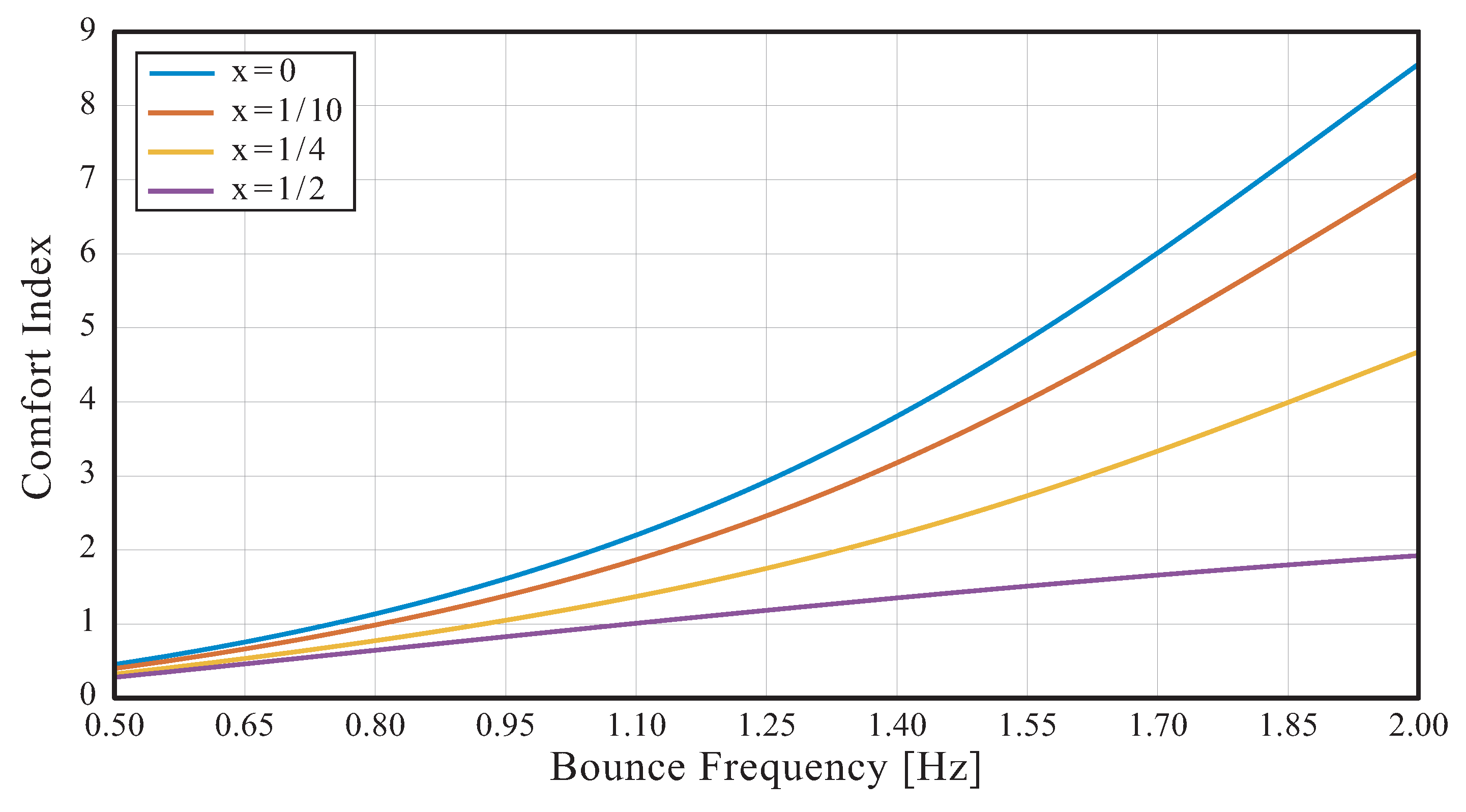
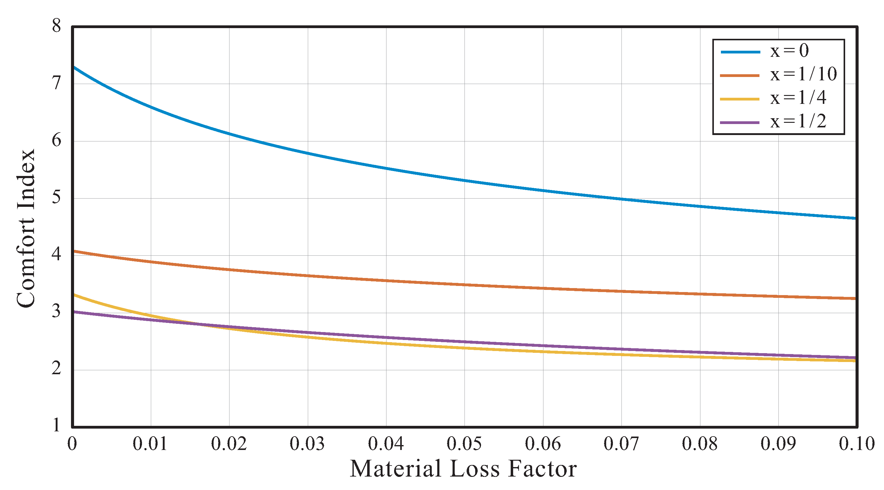
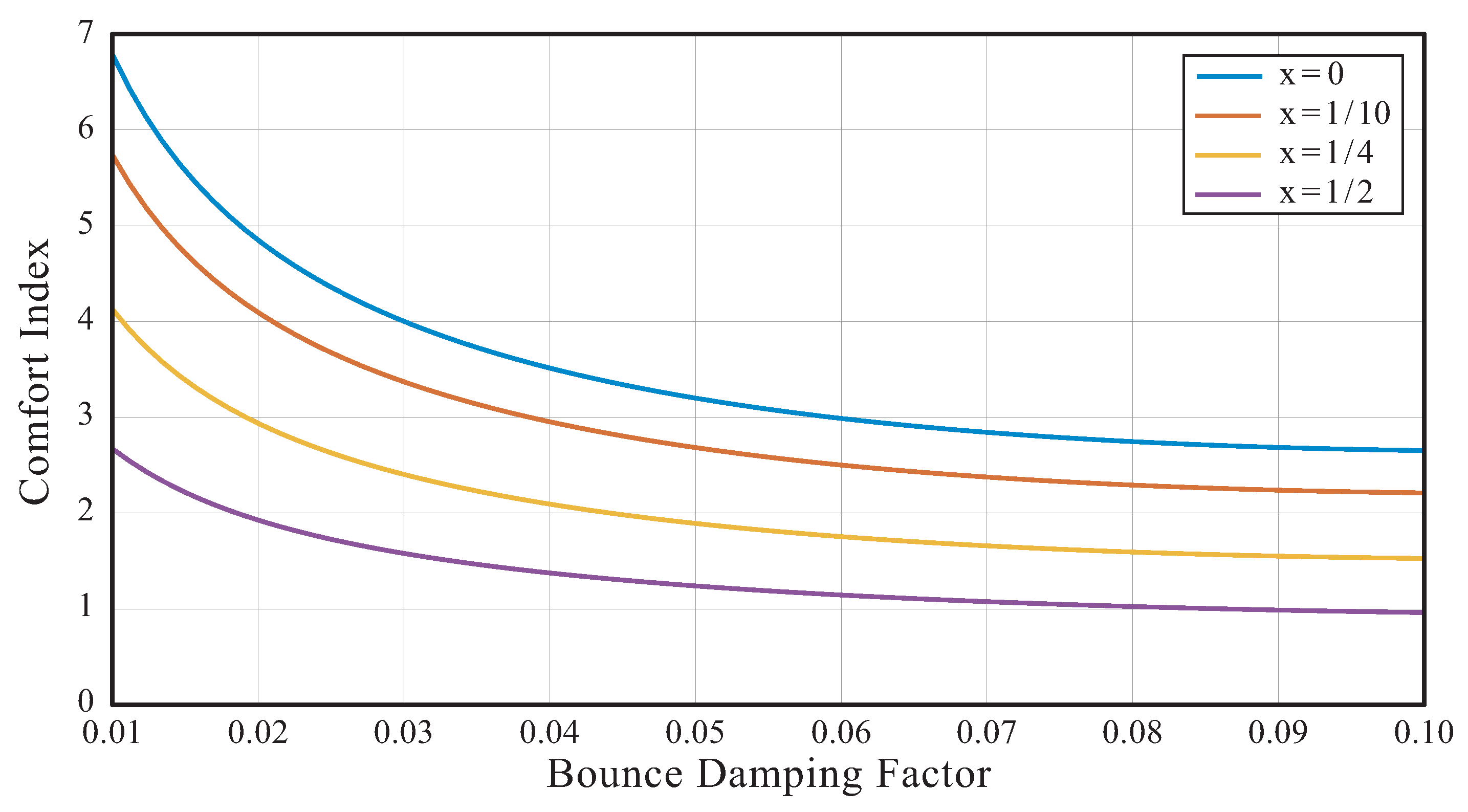
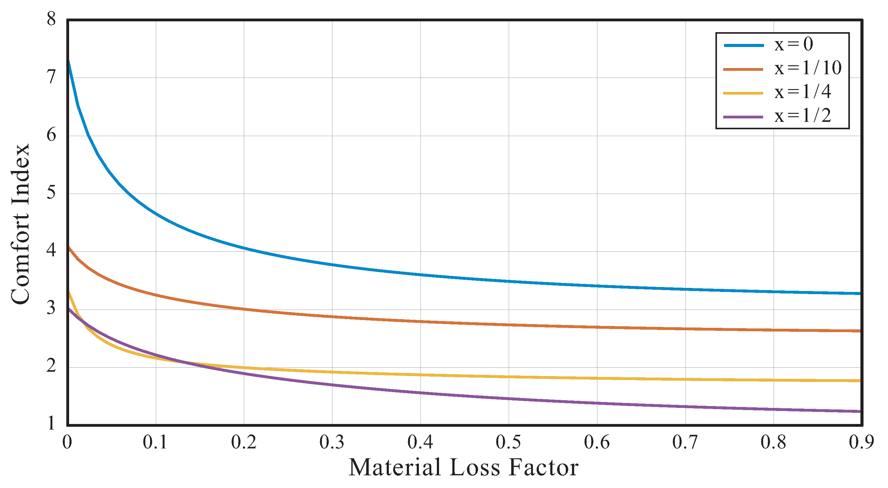
The influence of structural damping is depicted in Figure 10 and Figure 11. All parameters have the same values as in the previous analysis except for the bending frequency, which is now fixed at $f_3=8$ Hz, and the previously fixed material loss factor $\eta$, which is now free to vary from 0 to 10% (see Table 1). It can be seen that comfort improvements with an increasing loss factor are significant but not dramatic. These results indicate that railroad passenger car frames should have sufficient structural damping to improve comfort but that, at the same time, if the measures needed to increase the loss factor are too complicated, too costly, or too heavy (referring to the weight of the materials that would need to be added), the designer may pursue meeting specifications by other means rather than by increasing structural damping. The current trend to use viscoelastic materials to dampen vibrations is, in light of the simplified results presented in this paper, only advisable if the goal is to mitigate local vibrations of structural components rather than to dampen the overall vibration of the car. It could be argued that these statements may need to be revisited if it were possible to achieve much larger material loss factors. Nevertheless, as Figure 12 shows, marginal benefits go down as $\eta$ grows, becoming very small at most locations along the beam for $\eta >0.5$. Needless to say that the upper limit for the material loss factor in this figure has been stretched beyond what is feasible.

It was mentioned in the introduction that increasing the operational speed may have a negative effect on comfort. The assertion seemingly stands without proof. The rail irregularity spatial frequency content is mapped onto a larger range of frequencies for a higher velocity ($\omega =v\Omega$). As the speed increases, high spatial frequency harmonics are being pushed out of the interval of interest for comfort evaluation. However, at the same time, they are being replaced by low spatial frequency harmonics that, given the shape of typical input spectral density (Figure 2), are likely to have higher amplitudes. The consequence, therefore, is a larger response and reduced comfort. Nevertheless, the previous rationale forgets the fact that the mean square input displacement is not modified by the increase in speed and that, as a consequence, amplitudes are spread over a larger frequency range ($S_z\left(\omega \right)=(1/v)S_z(\Omega )$).

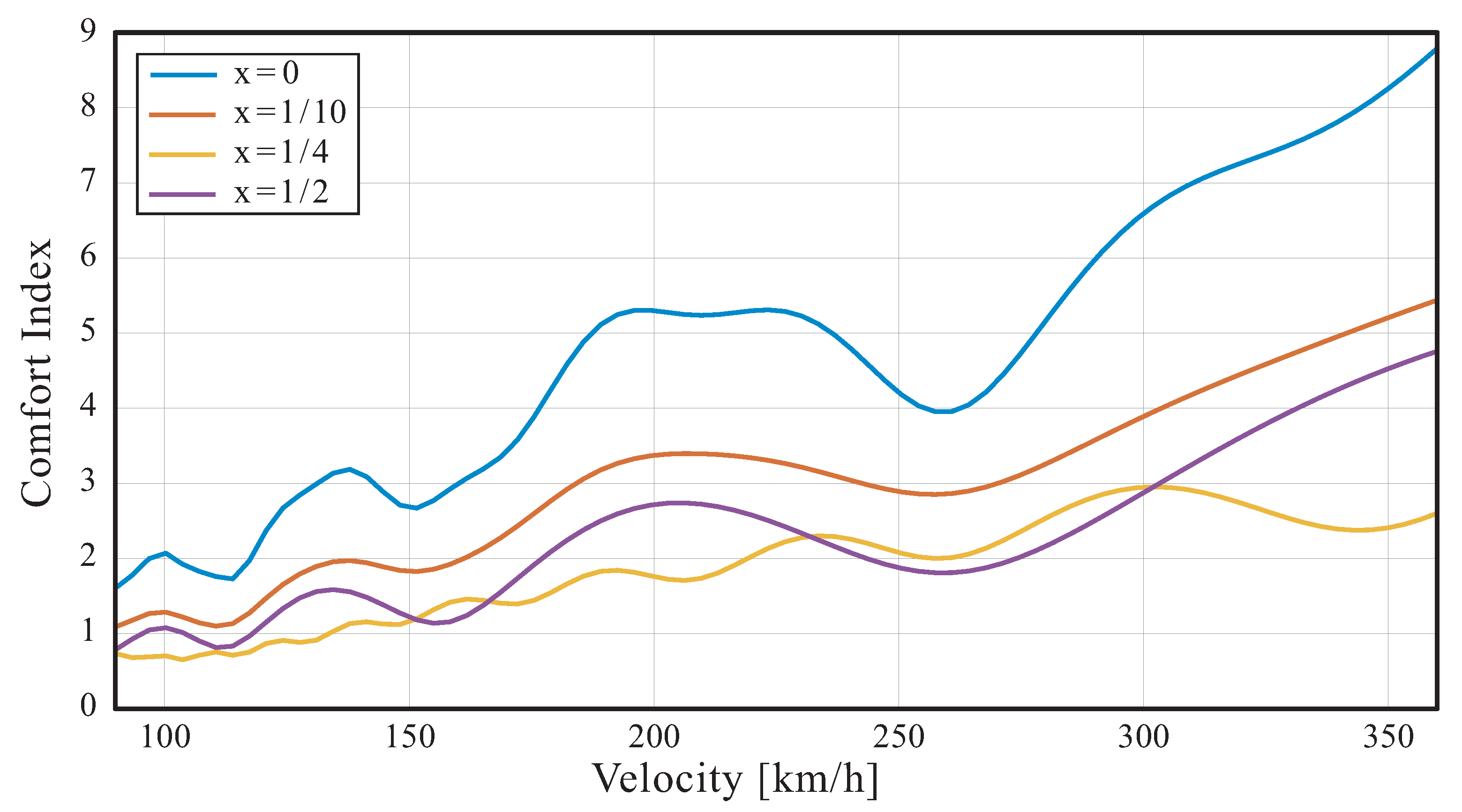
The two conflicting factors mentioned in the previous paragraph, along with the fact that the structural response is frequency-dependent, may (and, in fact, do) give rise to the non-monotonic evolution of comfort versus velocity. The influence of speed is depicted in Figure 13 and Figure 14. 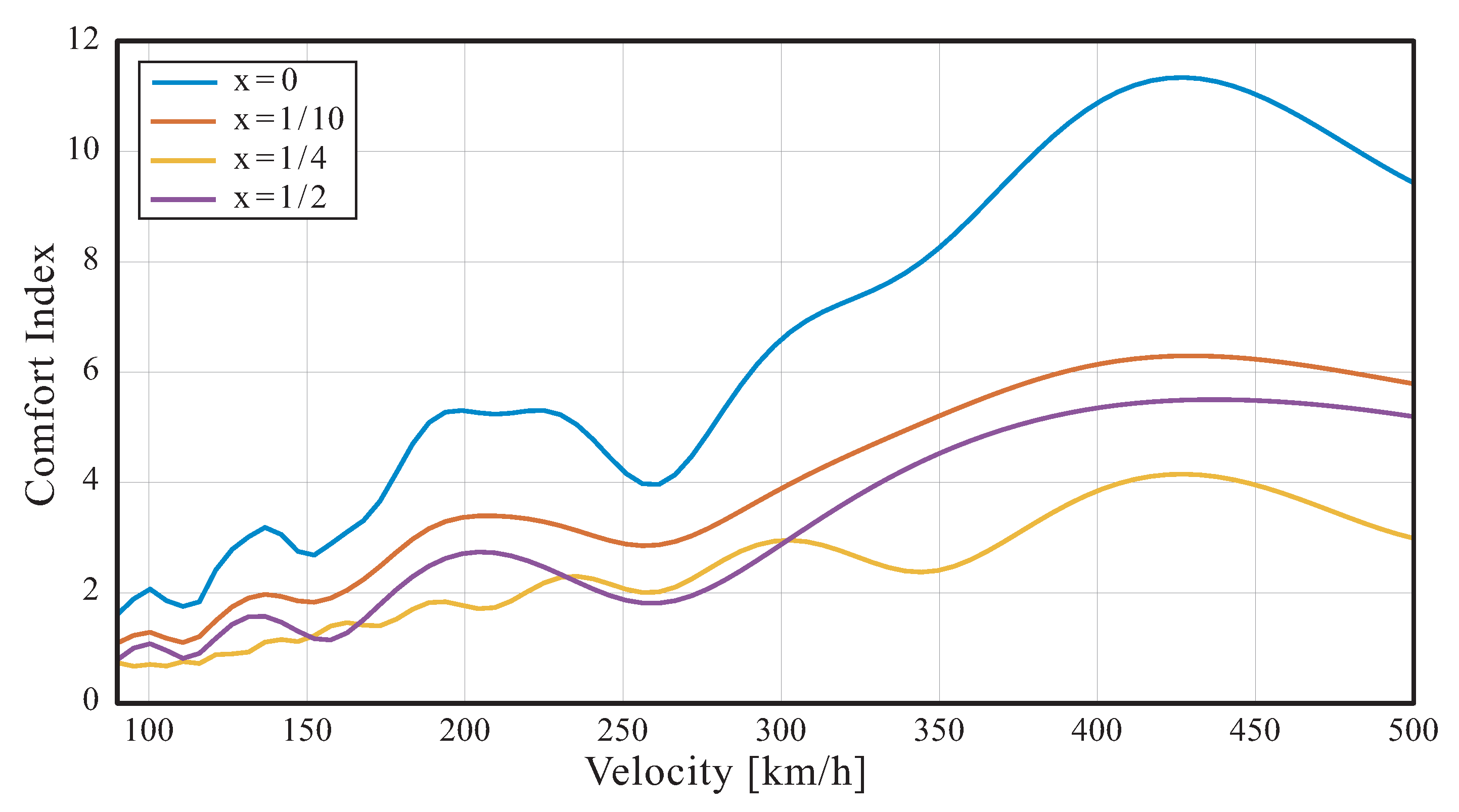All parameters have the same values as in the previous analysis except for the material loss factor, which is now fixed at $\eta =0.01$, and the previously fixed velocity v, which is now free to vary from 90 km/h to 360 km/h (see Table 1). The anticipated non-monotonic behavior is clearly seen in the plots. It is unfortunate that comfort deteriorates rapidly for speed increases that are now within reach (without major changes in infrastructure nor regulations) in typical high-speed train tracks (changing the maximum speed from 300 km/h to 360 km/m, for instance). As Figure 15 shows, velocity would have to be pushed beyond what is currently customary to start witnessing a new interval of comfort improvement with speed.

6. Conclusions

The main conclusions are: (a) using a viscous damping model overestimates the dissipation capacity of the structure, thus yielding too optimistic comfort levels; (b) determining comfort indexes from frequency domain analyses of beam models with complex moduli is not only feasible also but simple and straightforward. The analyses show that caution should be exercised when stiffening railway vehicle car structures. The general rule that “comfort improves as stiffness increases” breaks down for many stiffness intervals. Regarding the energy dissipation capacity of the structure, it has been shown that introducing moderate levels of structural damping noticeably reduces comfort indexes. Nevertheless, marginal benefits wane as the material loss factor grows, so a very large loss factor is seldom a cost-effective option.