
Gate Attentional Factorization Machines: An Efficient Neural Network Considering Both Accuracy and Speed


School of Mechanical and Information Engineering, Shandong University, Weihai 264209, China
*
Author to whom correspondence should be addressed.
Appl. Sci. 2021, 11(20), 9546; https://0-doi-org.brum.beds.ac.uk/10.3390/app11209546
Submission received: 22 August 2021
/
Revised: 30 September 2021
/
Accepted: 12 October 2021
/
Published: 14 October 2021
(This article belongs to the Collection Heuristic Algorithms in Engineering and Applied Sciences)
Abstract
:Nowadays, to deal with the increasing data of users and items and better mine the potential relationship between the data, the model used by the recommendation system has become more and more complex. In this case, how to ensure the prediction accuracy and operation speed of the recommendation system has become an urgent problem. Deep neural network is a good solution to the problem of accuracy, we can use more network layers, more advanced feature cross way to improve the utilization of data. However, when the accuracy is guaranteed, little attention is paid to the speed problem. We can only pursue better machine efficiency, and we do not pay enough attention to the speed efficiency of the model itself. Some models with advantages in speed, such as PNN, are slightly inferior in accuracy. In this paper, the Gate Attention Factorization Machine (GAFM) model based on the double factors of accuracy and speed is proposed, and the structure of gate is used to control the speed and accuracy. Extensive experiments have been conducted on data sets in various application scenarios, and the results show that the GAFM model is better than the existing factorization machines in both speed and accuracy.
1. Introduction
With the development and progress of social productivity and technology, the Internet is playing an increasingly important role. The continuous development of the Internet and the Internet of Things has brought exponential explosion of information, which is also the problem of information overload. It is under this background that the recommendation system comes into being, aiming to solve the problem of recommending appropriate items for users under massive information. It mainly studies the characteristics of users and items, and generates a better recommendation list by mining the potential or explicit links between users and items, so as to make recommendations for users. In this case, the recommendation accuracy becomes the most important factor to measure the quality of a recommendation system or model, and then becomes the core pursued in all stages of the development of the recommendation system.
The recommendation system is composed of three important modules: user modeling module, recommendation object modeling module and recommendation algorithm modeling module. Among them, recommendation algorithm modeling, also called recommendation model, is the core of the research. Recommended system model in the decades of development, there has been a qualitative leap, in the early days of the recommended model, the traditional collaborative filtering algorithm [1] undoubtedly occupies very important position, the recommendation algorithm based on user [2] and recommendation algorithm based on item [3] for a long time to occupy the mainstream of the recommendation algorithm, until now also doing well. The proposal of matrix factorization [4] provides the basis for the development of factorization machine [5], and logistic regression [6] based on classification problems has also become the core algorithm of classification problem model. Recommendation system has realized the real booming development after enter the deep learning time, the concept of the model is more important, the neural network is put forward and the development laid the foundation of deep learning model, Wide & Deep [7] model combines generalization and memorization, for the first time for subsequent model provides a new train of thought, to the recent time, image processing has become the hot of current recommender systems. The continuous evolution and development of CNN [8] and RNN [9] continue to promote the progress of image processing.
With the continuous development of the deep learning model, the complexity of the model is increasing. With the improvement of accuracy, the time complexity is also increasing, which has become one of the problems of the recommendation system model. There are many sources of time complexity. From a macro perspective, many hidden layers are added to the recommendation system model under deep learning. With the increasing of “depth”, the data processing time is prolonged; On the other hand, the use of Embedding technology [10] greatly increases the data processing time of the model, which is the main source of the time complexity of the model; Finally, the increasing size of the data set also causes the model to need more time to process the data. However, few models actively pay attention to solving the problem of speed, and the problem of time complexity is usually considered only when two models are compared. For example, the promotion and use of FNN [11] are precise because its model is relatively simple, and FM method is used to initialize parameters for the model, and the model has strong interpretability. However, FNN model itself is difficult to automatically extract information carried by high-order combination features, which means that it is not ideal for processing large data sets. Therefore, our research on model speed starts from the three factors mentioned before, and finally improves the model speed through processing of data, Embedding technology and model structure.
In this paper, we propose a Gate Attention Factorization Model (GAFM) based on the double factors of accuracy and speed, aiming at the problem of model speed proposed before. It can solve the time complexity problem of the model well and take into account the accuracy. The main contributions of this paper are:
(1) We have developed a model that takes into account both accuracy and speed, and can reconcile the trade-off between the two, improving the accuracy of the model to some extent and significantly reducing the time.
(2) We propose a flexible “gate” component that balances speed and accuracy by processing data. Readers can try to apply this component to their own models and combine it to produce good results.
(3) We have carried out experiments on data sets under different application scenarios. The experimental results show that GAFM has a certain improvement in accuracy and a significant improvement in speed compared with other factorization models, which proves the rationality and effectiveness of the model.
2. Related Work
Before the era of deep learning, the application of the most classic collaborative filtering algorithm can be traced back to the email filtering system in Xerox research Center in 1992 [12], but it was really promoted by Amazon in 2003 [13], which made it a well-known classic model, and still has its shadow in various models today. It was the development of collaborative filtering algorithm that promoted the emergence of matrix decomposition algorithm. In the 2006 Netflix Algorithm Competition [14], the recommendation algorithm based on matrix decomposition stood out and opened the prelude to the popularity of matrix decomposition. The core of matrix decomposition is expected to generate a hidden vector for each user and item, and make recommendations according to the distance between vectors. There are many methods to solve matrix decomposition, among which gradient descent has become the mainstream, and it also lays a foundation for the subsequent development of neural network. In view of the deficiency that matrix decomposition cannot be recommended comprehensively, the appearance of logistic regression is a good way to fill the loophole. At the same time, the foundation of neural network-“perceptron” concept formally appeared, has many aspects of significance. Logistic regression also has its disadvantages, that is, only using a single feature, the model expression ability is weak and do not use feature cross will not only cause information loss, but also sometimes significant errors. In order to solve the problem of feature crossing, a “violent” combination of POLY2 model was developed, which intersected all features in pairs and gave weights to all features, which inevitably brought high complexity. In order to optimize the complexity problem, Rendle proposed the FM model [15] in 2010, which used the inner product of two vectors to replace the single weight coefficient, that is, the implicit vector was introduced to better solve the problem of data sparsity. Specifically, let the feature be x and the weight w, and the basic expression of FM is:
By the introduction of implicit vector, the 𝑛 directly to level 2 weight and reduce the number of , when using gradient descent can greatly reduce the training costs.
With the continuous development of recommendation system, it finally ushered in a qualitative leap after the era of deep learning. In 2015, Auto Rec [16] proposed by Australian National University combined autoencoder and collaborative filtering, which really opened a new era of recommendation system. If Auto Rec is the initial attempt of deep learning, then the Deep Crossing model [17] proposed by Microsoft in 2016 is the complete application of deep learning system in recommendation system. Its biggest advance is to change the traditional way of feature crossing, so that the model is not only second-order crossover ability, can achieve deep crossover. The following models, such as Neural CF [18] and PNN [19], combine matrix decomposition and feature crossover with the deep learning framework. PNN emphasizes the diversification of feature Embedding crossover, and its defined inner product and outer product operations are more targeted. However, the obvious problem is that there’s a lot of simplification to optimize efficiency. In 2016, Google proposed the Wide & Deep model [20], which proposed the concepts of “memorization” and “generalization” for the first time, breaking the thinking of traditional models and directly developing a special system. The GAFM model proposed in this paper is also the evolution of Wide & Deep model to some extent. Among them, the memory ability can be understood as the ability of the model to directly learn and utilize the co-occurrence frequency of objects or features in the historical data, and the generalization ability can be understood as the ability of the model to transfer the correlation of features and explore the correlation between sparse or even never-appeared rare features and the final label. The Wide section is responsible for the model’s memory capability, while the Deep section is responsible for the model’s generalization capability. This combination of the two parts of the network structure, a good combination of the advantages of both sides, became an absolute hot. In the subsequent improvement of the Wide and Deep model, Deep FM model [21] in 2017 focused on the Wide part and improved the feature combination ability of the Wide part by using FM, while NFM model [22] in the same year focused on improving the structure of Deep and added feature cross pooling layer. Further enhance the data processing capability of the deep part. Additionally in 2017, AFM model [23] proposed by Ali introduced attention mechanism on the basis of NFM model, which once again contributed to the multi-domain integration of recommendation system.
As mentioned above, the recommendation system in the background of deep learning is committed to repeated innovation and improvement on the model, aiming to improve the accuracy of the model and produce better value in practical application. However, with the increasing complexity of the model, the time complexity of the model also increases. In this case, it is unreasonable to focus only on the prediction accuracy of the model, and the accuracy and time should be considered at the same time. For example, the point of PNN model is that it simplifies a lot of work of feature crossing, and it is not able to mining features well in terms of prediction, but its advantages lie in the simplification of model and high efficiency. On the contrary, AFM model has good feature combination crossover ability, but it is precise because of the introduction of attention mechanism, which further slows down the speed of the model, so in many large projects, it is considered to use PNN roughing and then further fining to save time. Therefore, in order to achieve the unity of accuracy and speed and solve the balance between them, this paper puts forward a new perspective to solve the problem and adds the concept of “gate” to optimize the structural model.
3. Materials and Methods
In this part, we will explain the basic structure and algorithm of the series of models related to our model in Part A; in part B, we will formally introduce the GAFM model proposed in this paper and give A detailed explanation of the algorithm; in Part C, we will make A summary of the model.
A. Related models and algorithms
(1) Wide & Deep
According to Google’s paper [20], the model is divided into four stages: Sparse Features, Dense Embeddings, Hidden Layers and Output Units. Sparse Features divide the input data into two parts, which are sent to the wide structure and the deep structure, respectively. The following three stages are the operation of deep. For the wide part, features are transformed by cross product to carry out feature combination, and the formula is as follows:
Among them, is a Boolean variable, when the ith feature belongs to the kth combined feature. is the value of the ith characteristic.
The Deep part is actually a feed-forward neural network. For category features, the original input is the feature string, and the sparse high-dimensional category features will first be converted into low-dimensional dense real vector, usually called embedding vector. These low dimensional dense vectors are fed into the hidden layer of the neural network in the forward transmission. Specifically, each hidden layer performs the following calculation:
where is the number of layers and f is the activation function, usually RELU, which is a common activation function of the form , and were the first layer of the activation of l, bias and weighting model. Finally, the wide and deep parts are combined through the full connection layer and finally output through the logical unit. For logistic regression models, the prediction of the model is:
where, Y is the binary classification label, is the sigmoid function, is the transformation of the original feature x, b is the bias term, and are the weight of the wide part and the deep part, respectively.
(2) Deep FM
As mentioned earlier, Deep FM improved on Wide & Deep by replacing the Wide part with FM. Specifically, the output of the FM part is the sum of the Addition unit and the Inner Product unit:
where, and . The Addition unit focuses on the first-order features while the Inner Product unit focuses on the second-order feature interaction.
(3) NFM
NFM is focused on improving the deep part of the Wide & Deep model, by introducing features cross pooling layer to solve the high order cross combination explosion problem, specifically, suppose is the set of all the characteristics of the domain Embedding, the characteristics of cross pooling layer concrete operation is as follows:
where, ⊙ represents the element product operation of two vectors, where the dimension operates as follows:
(4) AFM
AFM model introduces attention mechanism by adding attention network between feature cross layer and final output layer. The role of the attention network is to give weight to each cross feature. Specifically, the pooling process of AFM with attention score is as follows:
The indicate a score for the attention.
B. Explanation of GAFM
Since GAFM is proposed to solve the balance between speed and accuracy of the model, we first need to explore which factors affect the running time and prediction accuracy of the model. According to Sunil Ray’s 2015 article [24], some of the basic factors are shown in Table 1 below:
It can be clearly seen from the table that the complexity of model, the complexity of data and the weight calculation can significantly improve the accuracy of the model, but at the same time, all the influencing factors in the table will reduce the running speed.
According to the article, model complexity and data complexity are the primary factors affecting the accuracy of the model, which are the most intuitive and easy to manipulate. However, because these two factors have opposite effects on accuracy and speed, we should always be careful in choosing between them. The influence of Embedding is more impossible to ignore, which is often the factor that slows down the convergence speed of the whole neural network. The main reasons are as follows: (1) the number of parameters is huge, and most of the training time and calculation cost are occupied by Embedding. (2) The input vector is too sparse, which further reduces the convergence rate. Regularization and weight calculation have the same impact on the model and Embedding, which are the main factors to reduce the speed of the model.
It can be seen from the table that most of the factors conducive to improving the prediction accuracy will reduce the running speed of the model. Therefore, in order to ensure the first priority of accuracy, most models can only improve the time complexity of the model at the cost of. In order to alleviate this problem, the core idea of GAFM proposed in this paper is to start from the above main influencing factors, hoping to find a balance point to ensure the accuracy of model prediction and accelerate the operation speed. Based on this concept, we proposed the concept of “gate” structure and built the GAFM model.
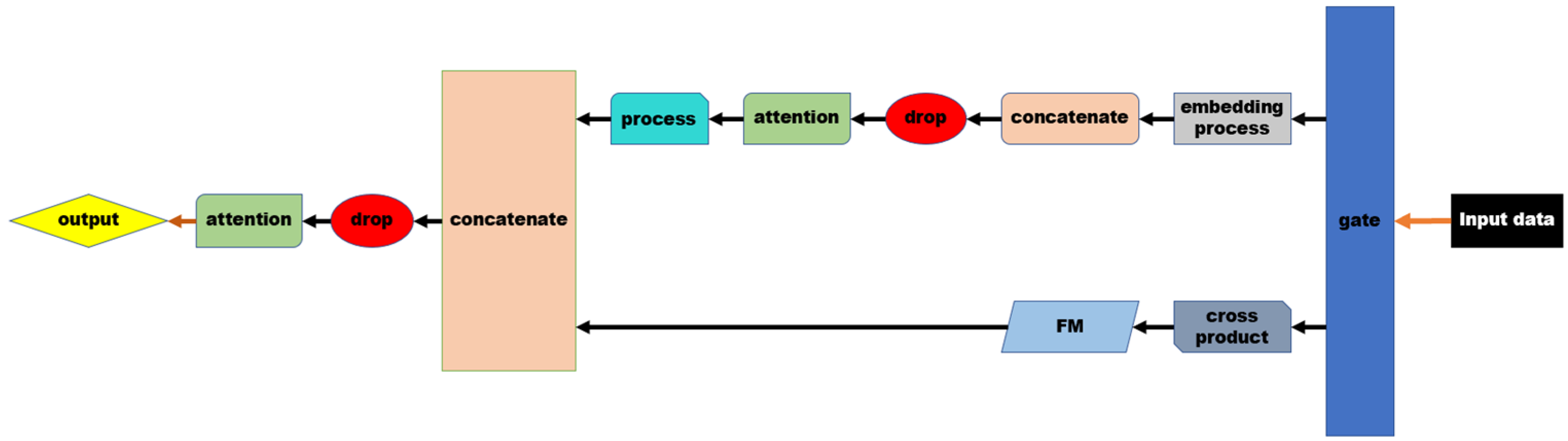
Figure 1 shows the main framework and data flow mode of GAFM. As mentioned above, GAFM is essentially an improvement of the series model of Wide & Deep. The input data is divided into two parts after processing by “gate”. The other is the wide processing part which is similar to Deep FM and replaced by FM part. Different from previous models, the drop layer is added to GAFM model, and the matching gate can reduce the time complexity. The roles and effects of the two attention layers in the model are also slightly different from those in AFM. In the following sections, the principles of the model are explained layer by layer.
(1) gate
Gate structure is the core structure of GAFM to improve the speed, and its main starting point is data complexity, that is, to solve the problem of model time-consuming from the perspective of data. In particular, the complexity of the data mainly comes from two aspects, one is the size of the data itself is too big, according to multiple studies by Smeden et al. [25,26,27], for large data sets, when data arrives at a certain scale will not continue to increase data has obvious improvement in accuracy, thus effectively compress the size of the input data reasonably is one of the ways to reduce the complexity of data; Embedding layer, on the other hand, the processing of greatly increased the running time, this is the major source of time complexity. Slow convergence speed and Embedding layer is the main reason of the parameters of the huge number and input vector is too sparse, this is mainly due to the category of the input feature vectors too much alone after hot coding vector dimensions is too high. Therefore, the processing of Embedding layer can be realized by reducing the vector dimension. However, this method will lose accuracy to some extent, because it will destroy the original data in exchange for a shorter time.
Starting from the two aspects mentioned above, we can acquire two processing formulas for gate structure, respectively:
a. Input data processing
Assuming that s for the input data size, for gate structure parameters, its value between 0 and 1, we can acquire the new data size as follows:
Using Equation (9), the input data can be compressed to a customized degree, and the parameter G is the hyperparameter.
b. Embedding layer processing
Assuming that the number of feature dimension of the input vector is n and is a gate structure parameter whose value is between 0 and 1, it has the same meaning as above, so subscripts 1 and 2 are used to distinguish the two variables. The dimension dim of Embedding can be obtained as follows:
Equation (10) can be used to reduce the vector dimension of Embedding layer, and parameter G is a hyperparameter.
In general, because of the large adjustable range of parameter G, it is often not necessary to use the above two methods at the same time in practical applications, so a parameter λ is introduced to combine the two formulas:
Among them, λ takes 1 to realize compressed data, λ takes 0 to realize compressed Embedding.
(2) drop
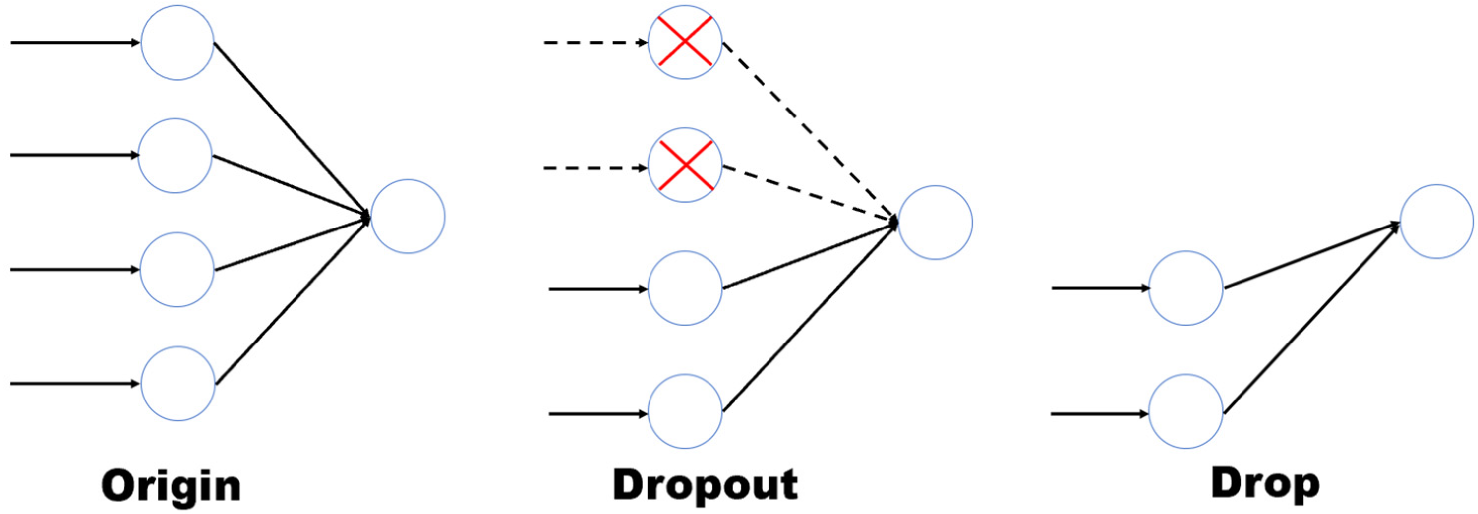
Drop structure is another structure we proposed to speed up the model. Its starting point is to reduce the complexity of the model, that is, to change the complexity of the model from the perspective of network structure. Specifically, we apply the pruning idea of the neural network to the drop structure. Given a parameter d with a value between 0 and 1, the neural network only keeps the neurons before d and drops the parts after (1-d). It should be noted that the drop structure is not the same as dropout. Dropout only inactivates random neurons and does not change the network structure of the neural network, so it can only prevent overfitting and even prolong the running time. The idea of pruning is to directly cut some neurons to simplify the network structure.
The essential difference between Dropout and Drop can be clearly seen in Figure 2. From an implementation perspective, there are two Drop structures in the GAFM model, one after the two fully connected layers, to solve the balance problem when entering large data, assuming that the matrix of fully connected neurons is concat_embeds, the number of neurons input is n, and the value of parameter D is between 0 and 1, then:
(3) attention
The attentional mechanism is a technology that has recently become popular in recommendation systems, and it comes from the most natural human habit of selective attention. The most typical example is when a user is browsing a web page, they will selectively pay attention to certain areas of the page and ignore other areas. It is based on this phenomenon that good benefits are often achieved when the influence of attention mechanism on prediction results is considered in the modeling process.
Similar to the feature crossover of the traditional model, for example, NFM, the feature Embedding vectors of different domains are intersected by the feature crossover pooling layer, and then each crossover feature vector is added and input into the output layer composed of multi-layer neural network. The key to the problem is the addition and pooling operation, which is equivalent to treating all the intersecting features equally, regardless of how different features affect the result, and in fact dissolves a lot of valuable information.
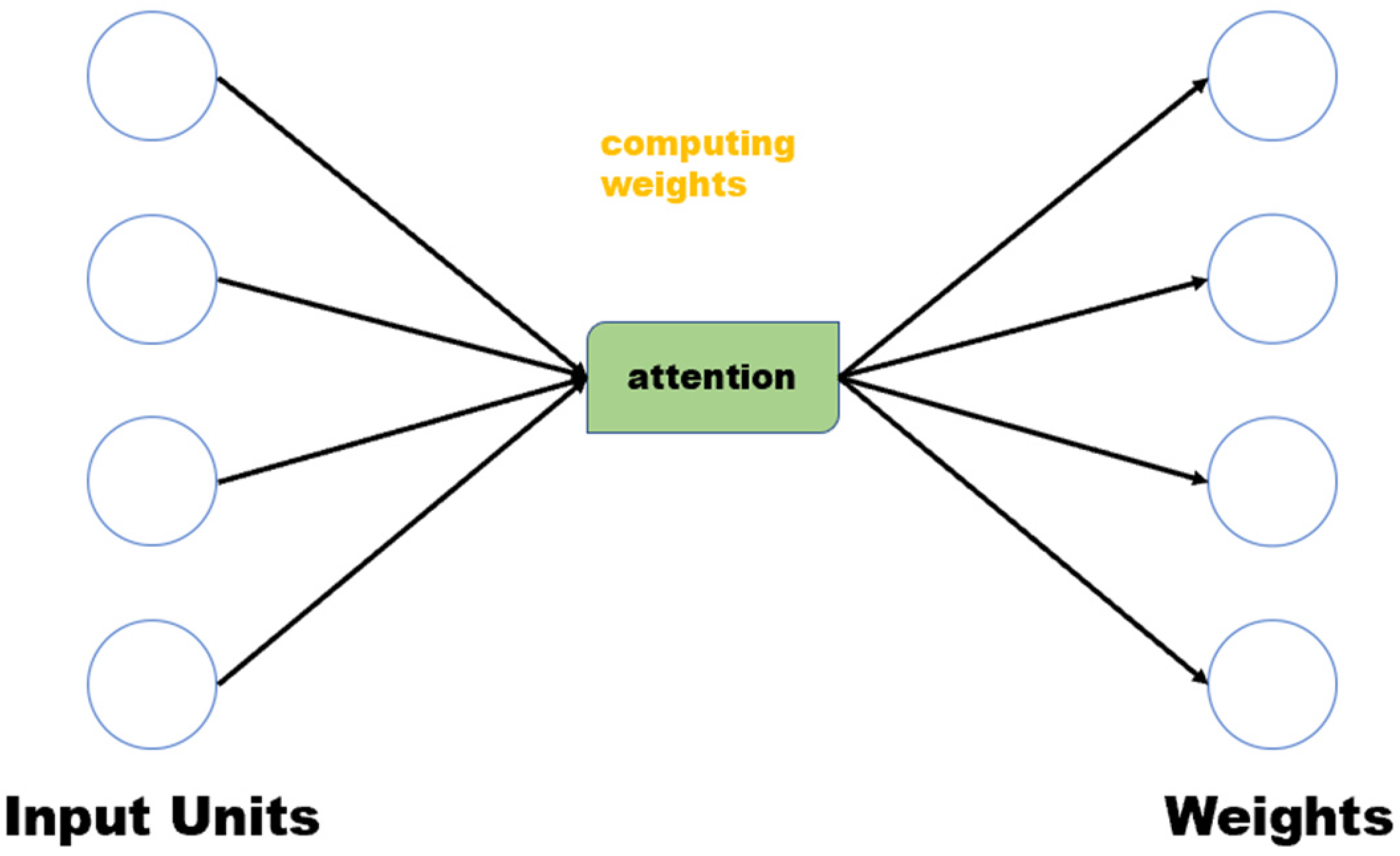
Therefore, the application of attention mechanism in the model is mainly to assign a weight to each input neuron, which can reflect the different weights of the input of different neurons. Specifically, after the drop layer, the attention layer in GAFM calculates the corresponding weight of the input of each neuron through the Sigmoid function. Next, you multiply that weight times the input vector to acquire the new weighted vector.
As shown in Figure 3, the corresponding weights of the input neurons are calculated by attention. Specifically, assume that the input is input_embeds, the sigmoid function is 𝜎 (), and the calculated weight is score:
The newly empowered neurons are:
(4) Other network structures
The other components of GAFM function are the same as the traditional model. The Wide part of the FM follows the processing of the Deep FM model, and the Process layer is actually composed of many hidden layers. Readers can design the structure of the Process layer to process their own data according to their needs, depending on the structure and depth of course. The effect of the model will have different results.
C. The summary of GAFM model
In general, the large framework of GAFM is based on the memory + generalization idea of Wide & Deep model, and new components are added on this basis. In the Wide part, the idea of Deep FM model is followed to strengthen the crossover capability of features and better explore the potential factors of features. In the Deep part, drop layer and Attention layer are added, and the data is processed by the Process layer. GAFM is proposed to solve the balance between accuracy and speed. How can this be achieved in the model? We know from the analysis that there are two aspects that affect the complexity of the model: Data complexity and model structure complexity. Therefore, gate and drop structures proposed by us are, respectively, used to solve the problems of data and structure. Attention is proposed to increase the prediction accuracy of the model, although it is on the premise of sacrificing certain speed.
Therefore, GAFM has the following advantages over other models:
(1) Compared to Deep FM model or AFM model, it has faster speed and relatively high accuracy, which has a good time advantage when dealing with large feature projects.
(2) Compared with models such as PNN and FNN, it has higher accuracy and a relatively high degree of freedom in time, and can have a good effect in the context of high accuracy.
(3) Compared with other traditional models, GAFM has both high accuracy and faster speed, with a significant performance improvement.
4. Experiments and Results
A. Settings
Before conducting experiments on our proposed model, we raised two core questions, around which we conducted experimental verification:
Q1. Does our model have a significant improvement in prediction accuracy over other existing models?
Q2. Does our model have a significant increase in speed compared to other existing models?
(1) Data set
In the selection of data sets, we choose three different data sets. The first data set is the data extracted by Becker from the 1994 census database [28]. Each data set records a person’s age, work and other data, and income can be predicted by using this data set. The other two data sets came from the public data and the Movielens [29] series. We selected data sets of 1 M and 10 M, respectively, to achieve multi-classification of movie ratings.
The first dataset has 14 features, which are numerical features age, education_num, capital_gain, capital_loss and hours_per_week. Category features include workclass, education, marital_status, occupation, relationship, race, gender, native_country and income_bracket.
For the Movielens dataset, we took category features gender and genres, numerical features user_id, movie_id, age, timestamp and occupation.
(2) Evaluation methodology
For model evaluation mainly from two aspects, the first is the prediction accuracy, we divide the data sets into training set and test set according to a certain scale, the model of training in the training set, evaluation of the effect on the test set, specific evaluation methods for, we will acquire the results of prediction and a numerical and acquire the total deviation. The proportion of the remaining correct value in the total value is the accuracy. For the evaluation of time efficiency, we statistically calculated the total time consuming from training to evaluation completion of the model, and made a horizontal comparison.
(3) Baselines
We ended up comparing our model to the following:
(a) Wide & Deep: As an original series of models, it will be used as a basic standard for the Wide & Deep model.
(b) PNN:PNN model plays an important role in machine learning tasks, and its fast speed makes it an important object of speed indicator.
(c) AFM:AFM model adopts attention mechanism, and the prediction accuracy of the model is further increased. We take its selection as the main comparison object of accuracy
(4) Parameter setting
In the GAFM model, the values of the two core parameters drop and g are the focus of our experimental discussion, considering that the parameter value is meaningless when it is 0, and the result increases too fast when the parameter value is too low, we select the values with a step of 0.01 in the range from 0.1 to 1, respectively, which convenient for experiment and values are the same, while other parameters are fixed parameters of the model. In the process structure, we set the Dense layer of 512, 256 and 128 units, respectively. The value of batchsize is 128, and the value of epochs is 15.
B. Accuracy assessment (Q1)
In order to answer the first question we raised, that is, the evaluation of model accuracy, we present the prediction accuracy effect of the model on different data sets in this part, and give the corresponding conclusions.
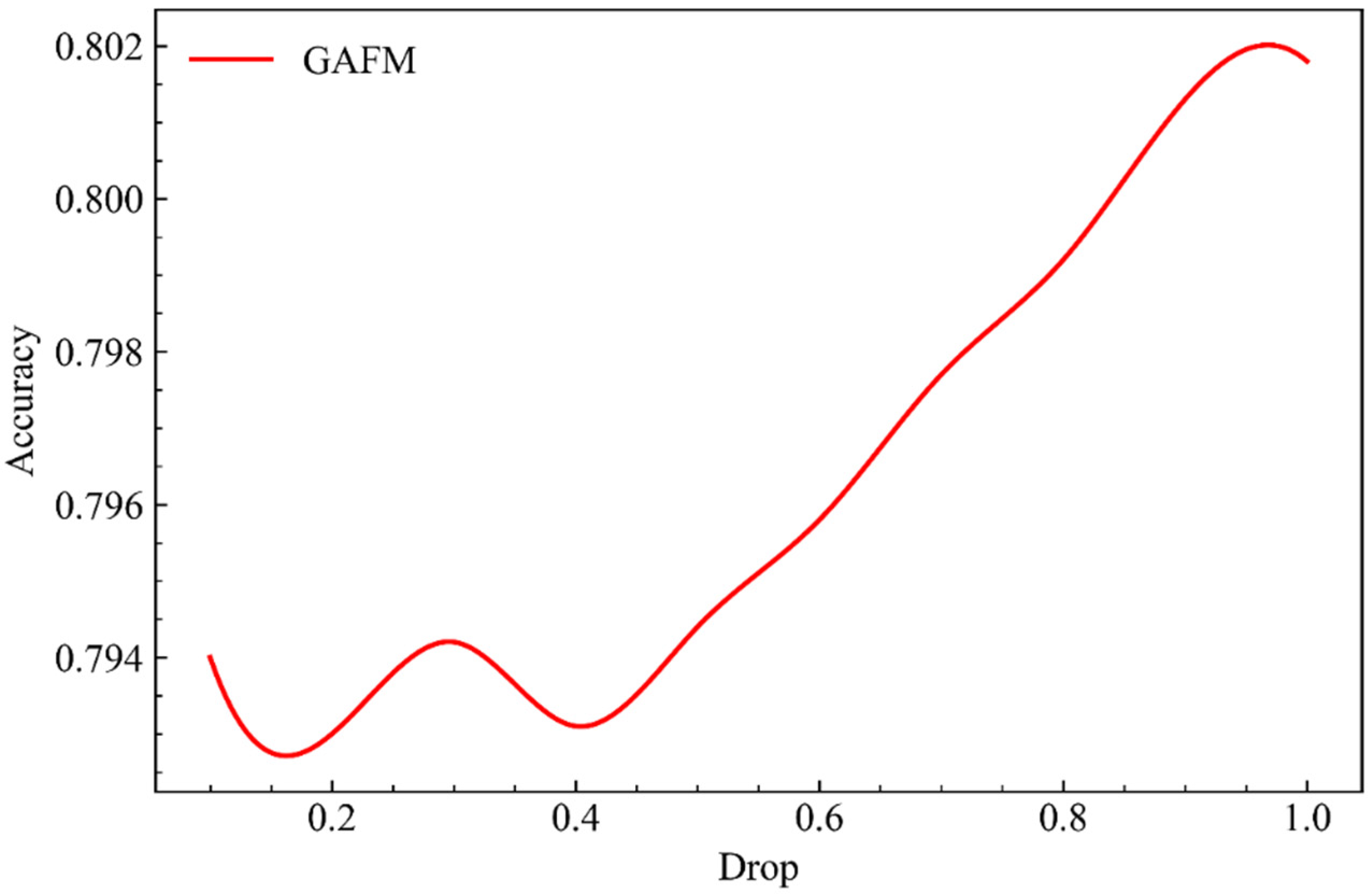
(1) The first is the experimental results on dataset 1:
As can be seen from Figure 4, when parameter g, namely gate structural parameter, remains unchanged, with the increase of parameter drop, the accuracy of GAFM running on dataset 1 increases slowly at first and then fast.
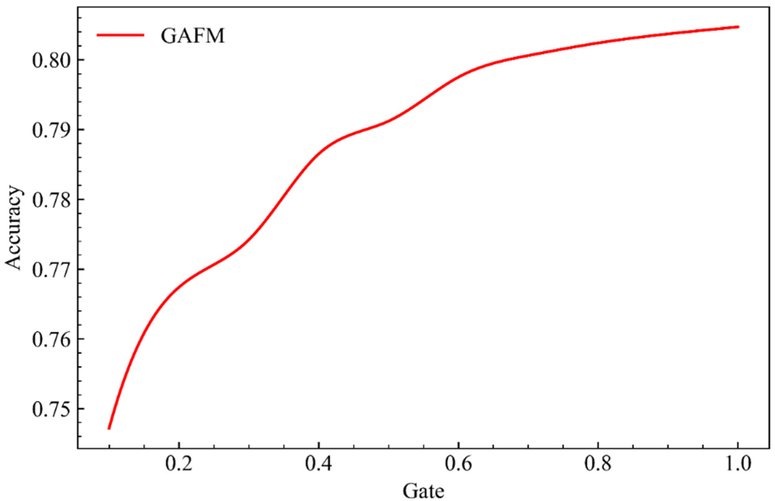
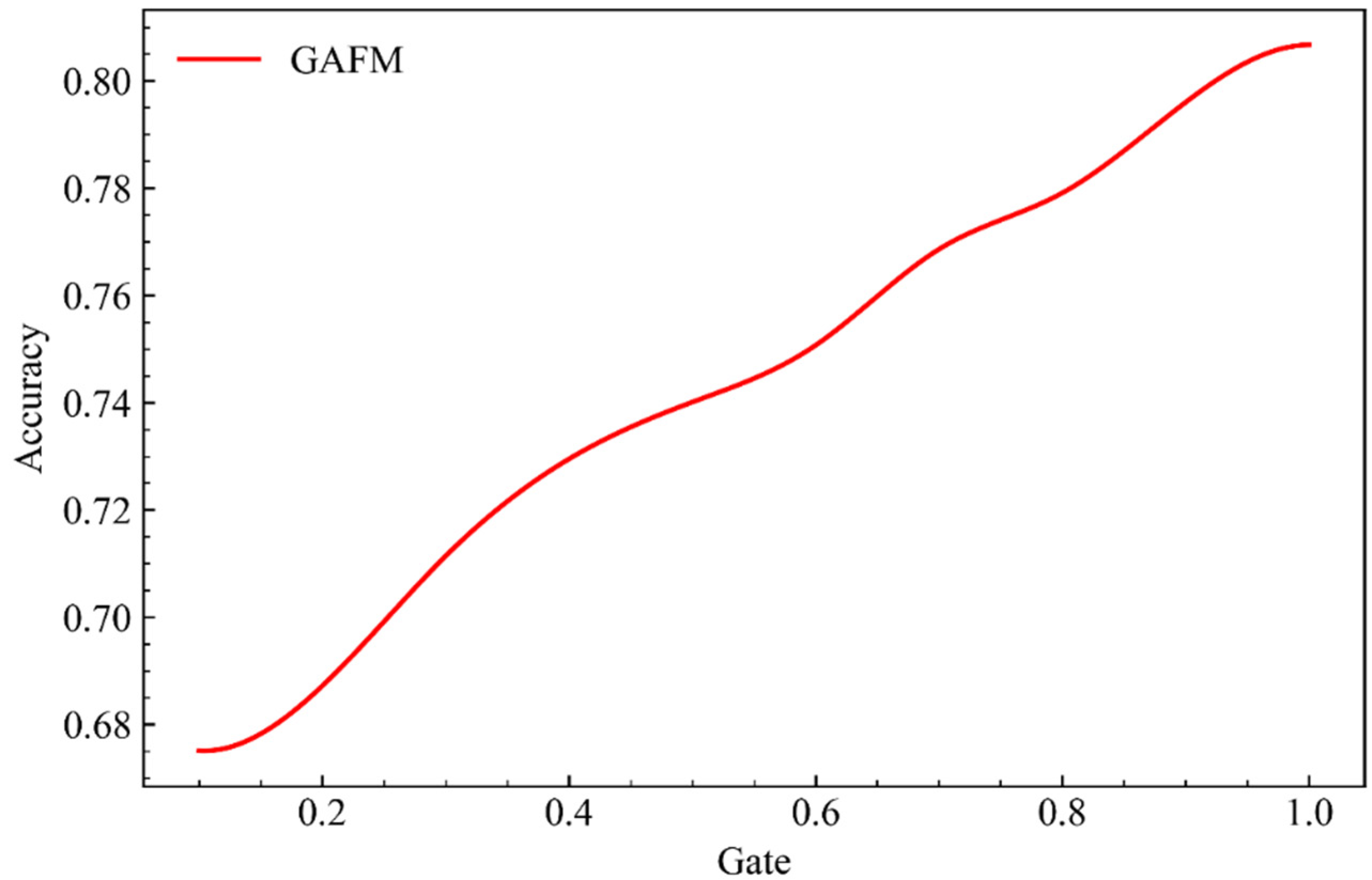
As can be seen from Figure 5, when parameter drop remains unchanged, with the increase of parameter g, the accuracy rate of the model on dataset 1 shows a rapid but slightly fluctuating increase.
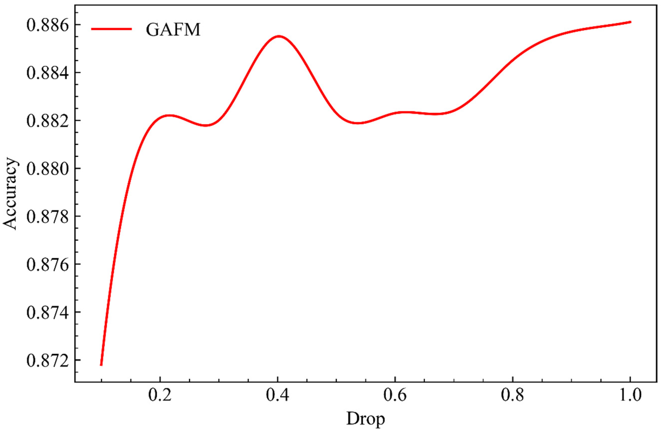
(2) The second is the experimental effect on dataset 2, which is the Movielens dataset with the size of 1 M:
As can be seen from Figure 6, under the condition that parameter g remains unchanged and parameter drop keeps increasing, GAFM performs slightly worse on dataset 2 than on dataset 1. It fluctuates greatly before parameter drop is 0.5 and then begins to grow rapidly.
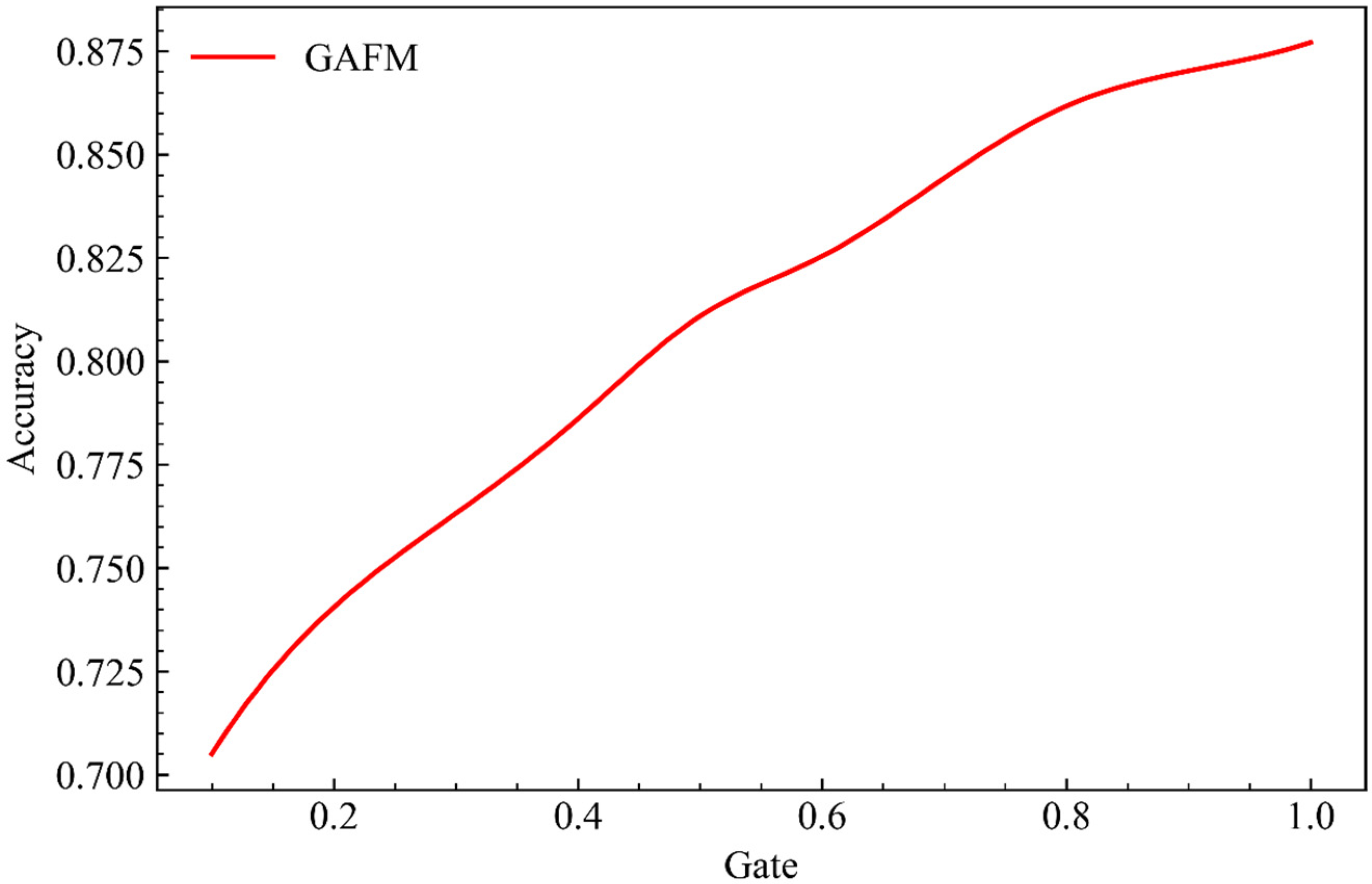
As can be seen from Figure 7, when parameter drop remains unchanged and parameter g increases, the performance of model dataset 2 is relatively stable without significant change in growth rate.
(3) Finally, the experimental results on dataset 3, namely the Movielens dataset of 10 M size:
As can be seen from Figure 8, due to the large increase in the data size of dataset 3, the accuracy of the model is generally good but fluctuates greatly in the process of parameter g remaining unchanged and parameter drop increasing.
It can be seen from Figure 9 that, different from the previous experiment, the accuracy of the model improved very steadily when parameter drop remained unchanged and parameter g kept increasing, which indicated that parameter g had better robustness compared with parameter drop.
(4) Conclusions:
In this section we present the GAFM in drop and g under the influence of two parameters, forecast accuracy, can be seen from the results of the drop and g is closely relative to both parameters and accuracy, but the drop parameters have significant volatility, and the results of the range is significantly smaller than g parameters under interval, the results of the influence of the parameter g for accuracy is stabler and clearer.
C. Evaluation of speed (Q2)
In this part, corresponding to the previous part, we mainly show the effect of the model’s running speed under different data sets, and give corresponding conclusions.
(1) The first is the experimental effect on data set 1:
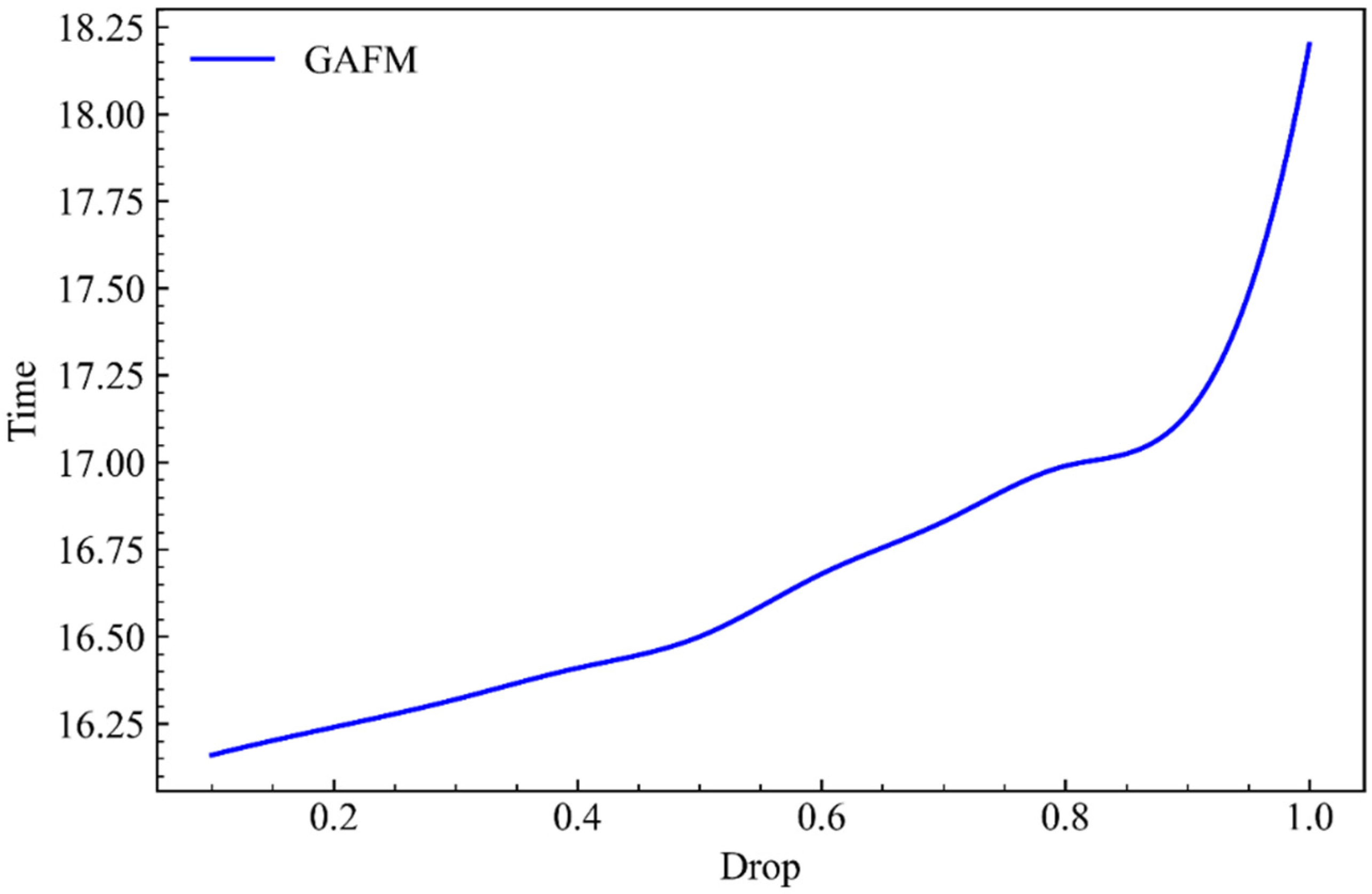
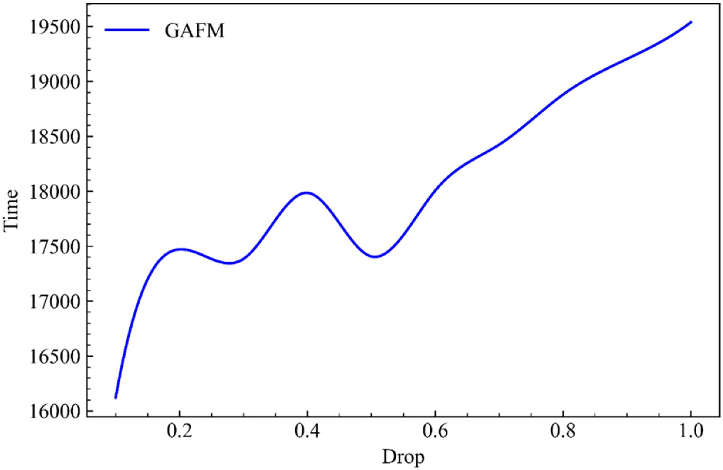
As for the experiments related to speed, we present them with intuitive running time, which indicates that the faster the growth in the figure, the greater the influence and limitation on speed.
As can be seen from Figure 10, when parameter g remains unchanged, the growth rate of the model’s running time on dataset 1 gradually increases with the increase of parameter drop.
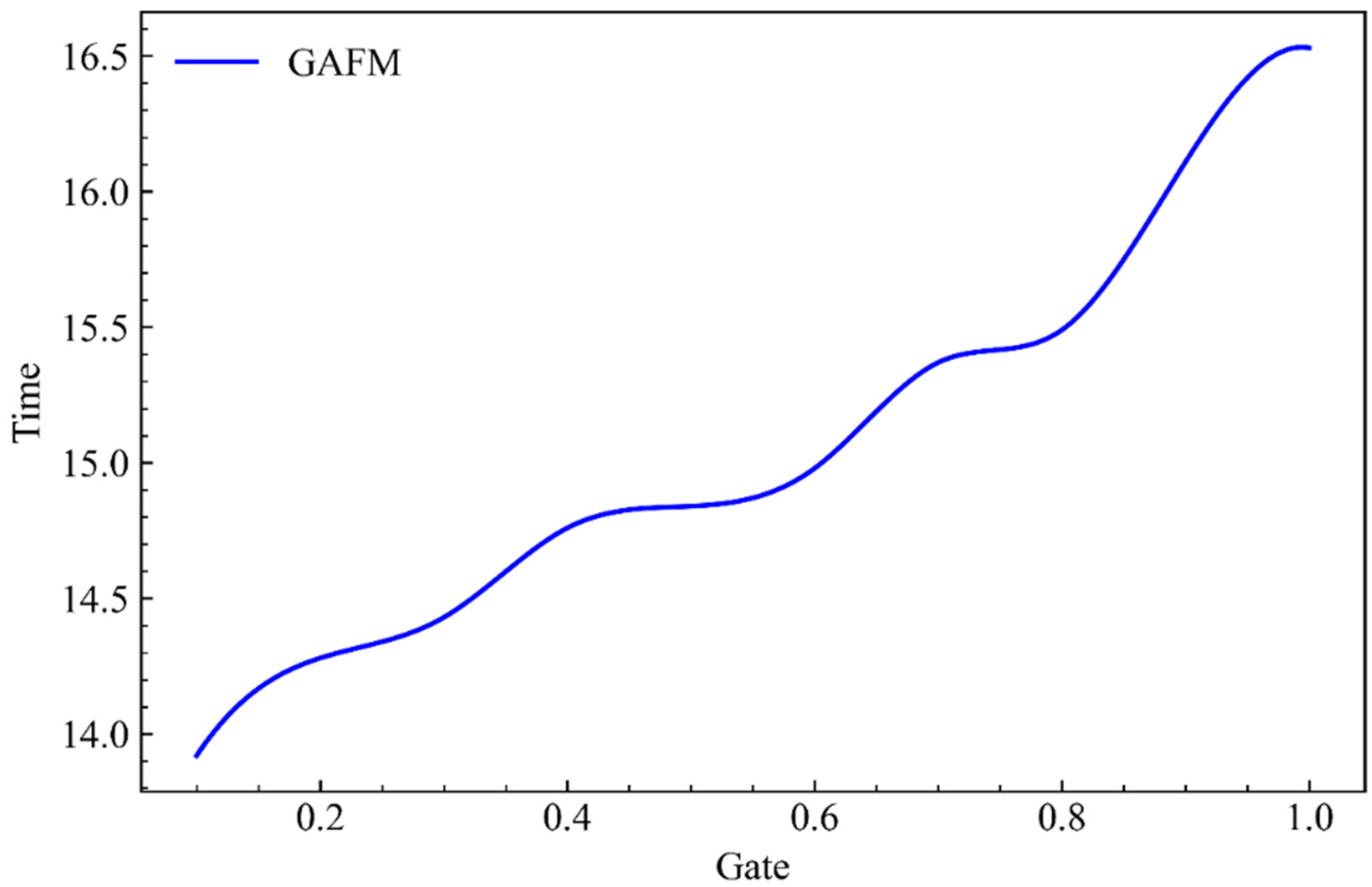
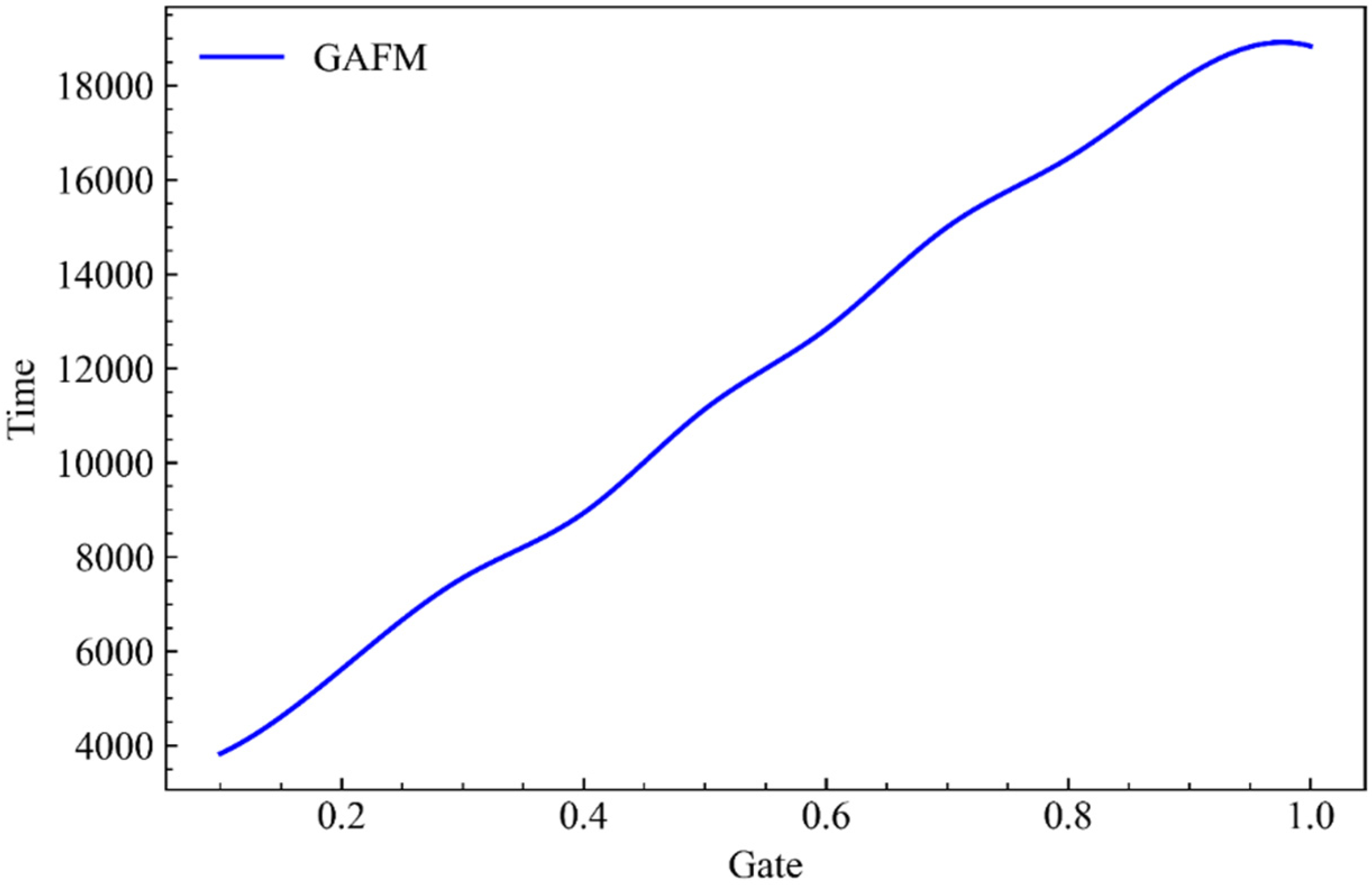
As can be seen from Figure 11, when parameter drop remains unchanged, the running time of the model increases with the increase of parameter g.
(2) The second is the experimental effect on dataset 2, which is the Movielens dataset with the size of 1 M:
As can be seen from Figure 12, in data set 2, when parameter g remains unchanged and parameter drop keeps increasing, we can find that the results presented by the model are almost consistent with the experiments related to accuracy, but with more unstable fluctuations.
As can be seen from Figure 13, when parameter drop remains unchanged and parameter g keeps increasing, the model presents a very stable time linear growth under dataset 2.
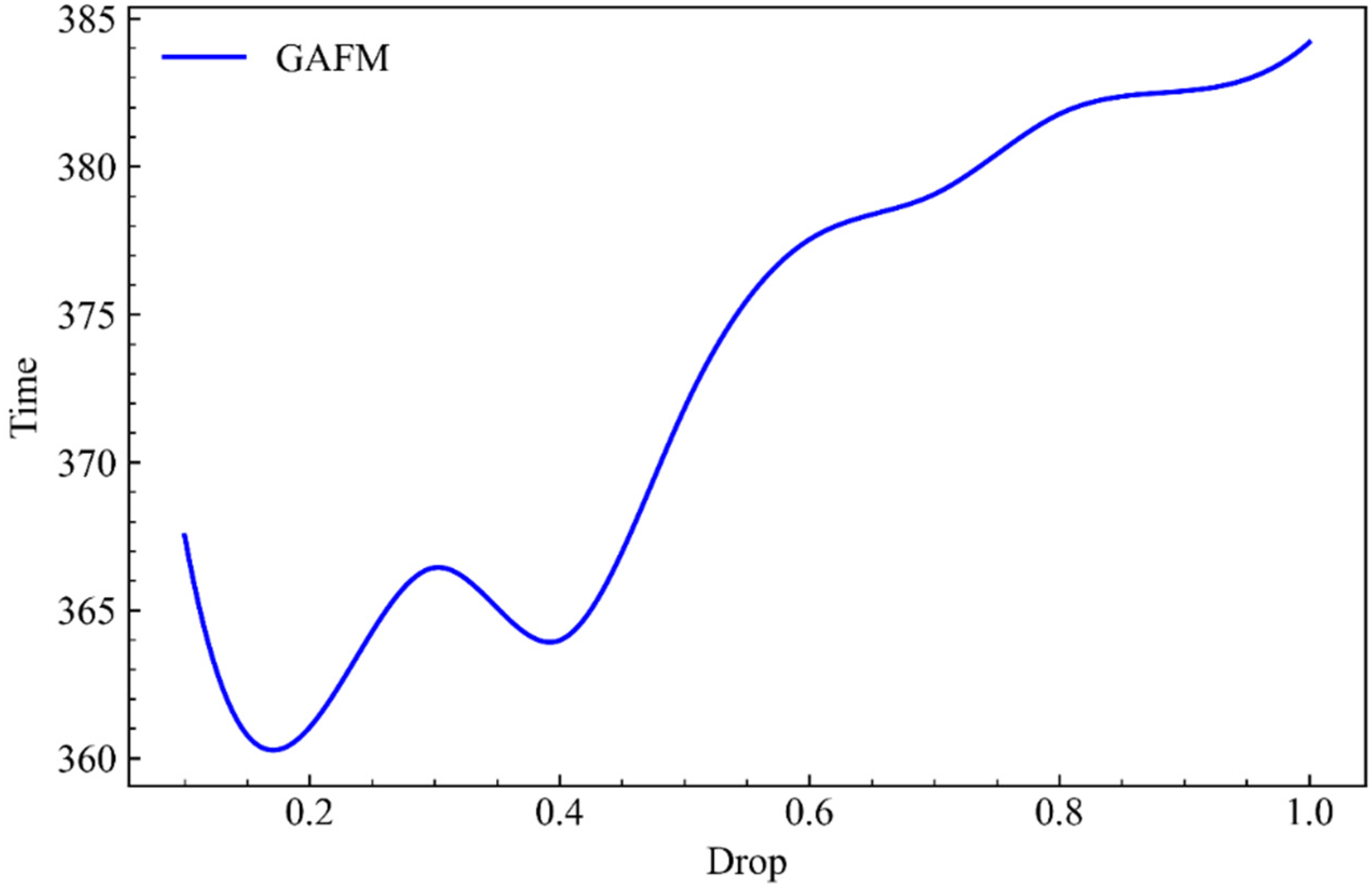
(3) Finally, the experimental results on dataset 3, namely the Movielens dataset of 10 M size:
From Figure 14, we can still find that time has a great relationship with the change of accuracy. Similar to the experiment of accuracy, when parameter g remains unchanged and parameter drop keeps increasing, the model has a large fluctuation time growth under dataset 3.
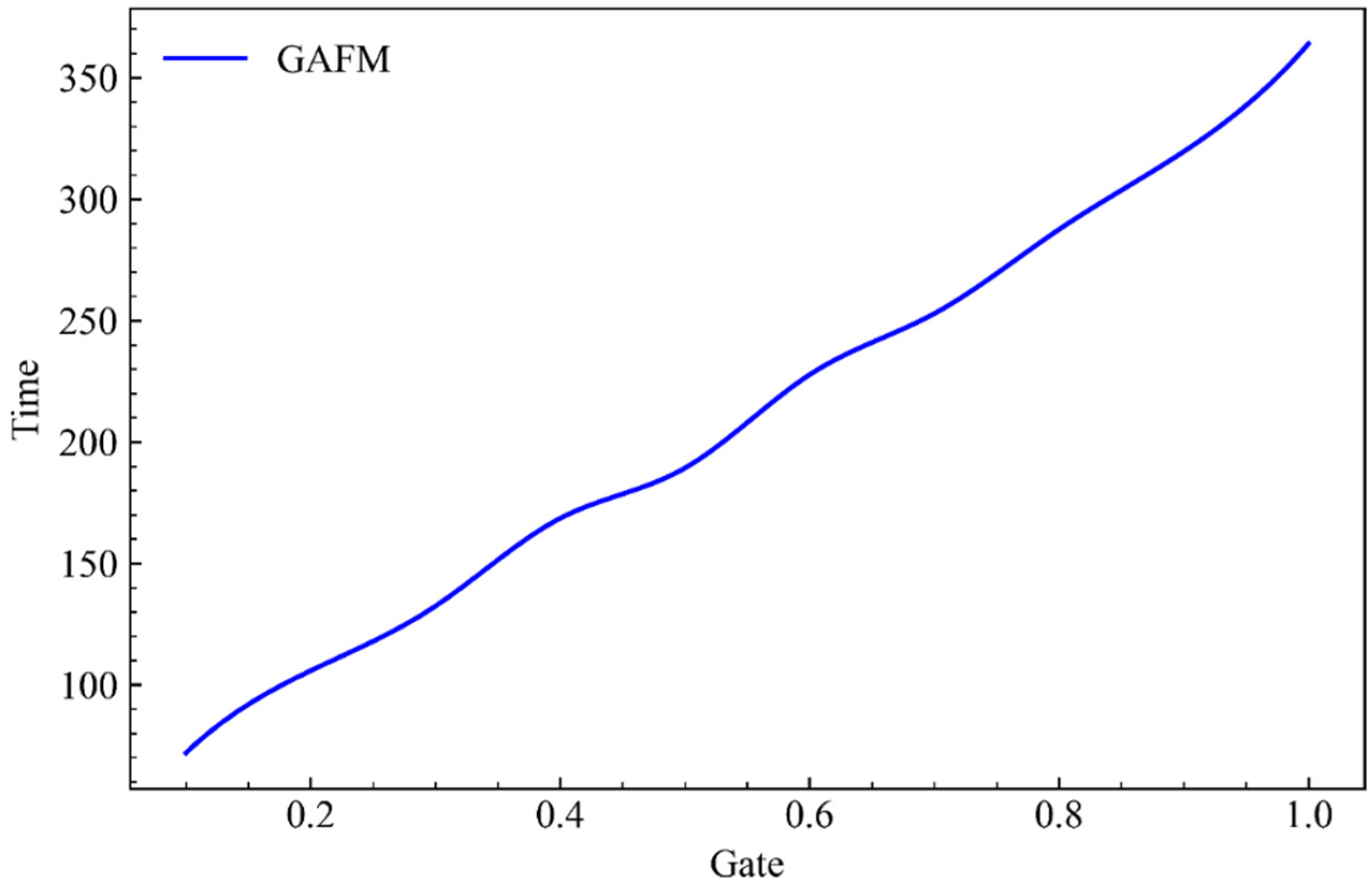
As can be seen from Figure 15, when parameter drop remains unchanged and parameter g keeps increasing, the running time of the model presents a stable linear growth.
(4) Conclusions:
In this part, we give the running time of GAFM under the influence of the two parameters drop and g. It can be seen that, similar to the accuracy, the impact of the two parameters on the running time is positively correlated, that is, negatively correlated with the speed. The impact of drop is also volatile, and the impact on the time is less than that of the parameter g. It can be seen that the influence of parameter g is more stable and significant.
D. Horizontal comparison
In this section, we compare the effects of GAFM with other models, and show the growth of one model against the benchmark.
(1) Experimental effects on dataset 1:
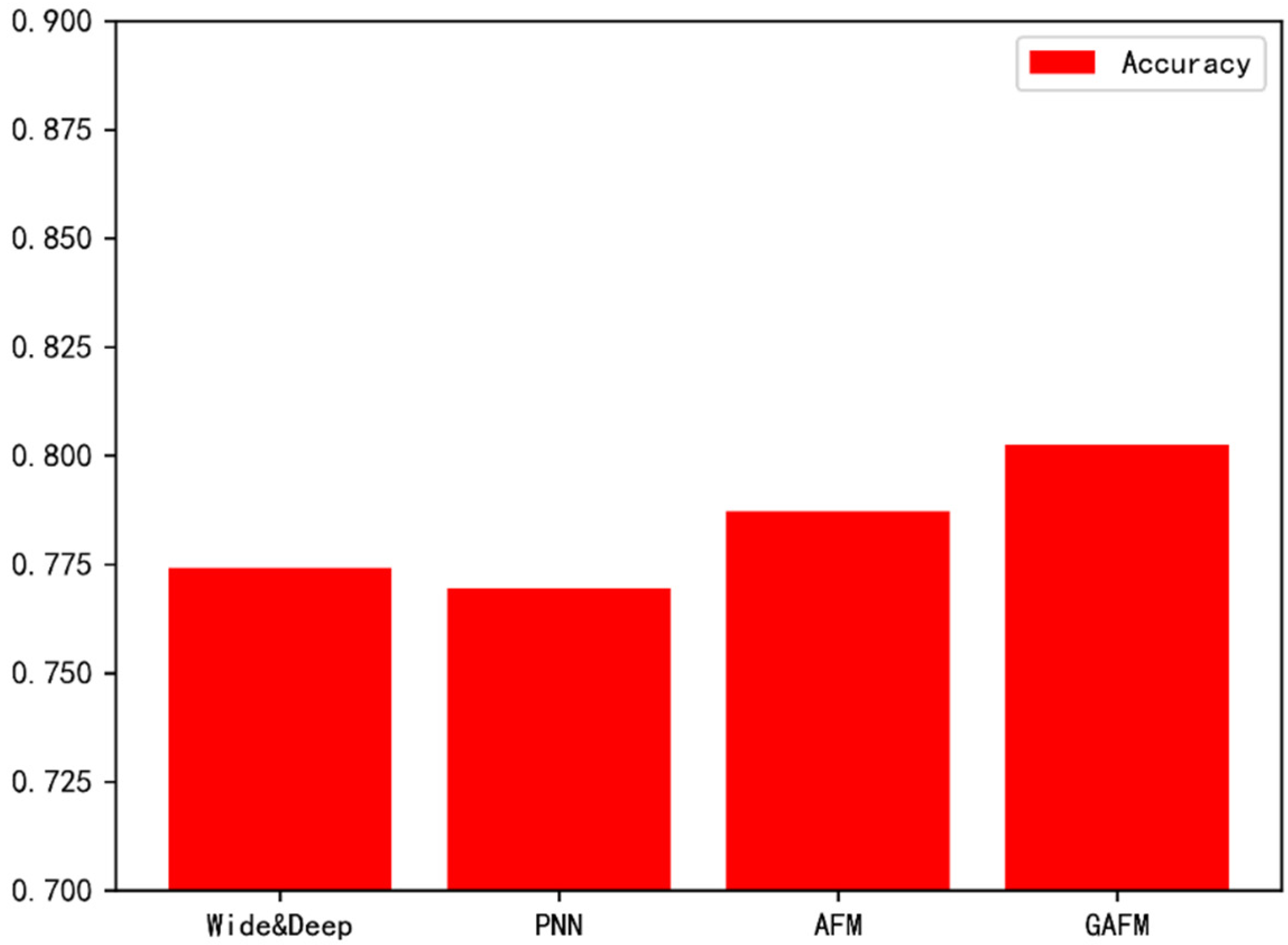
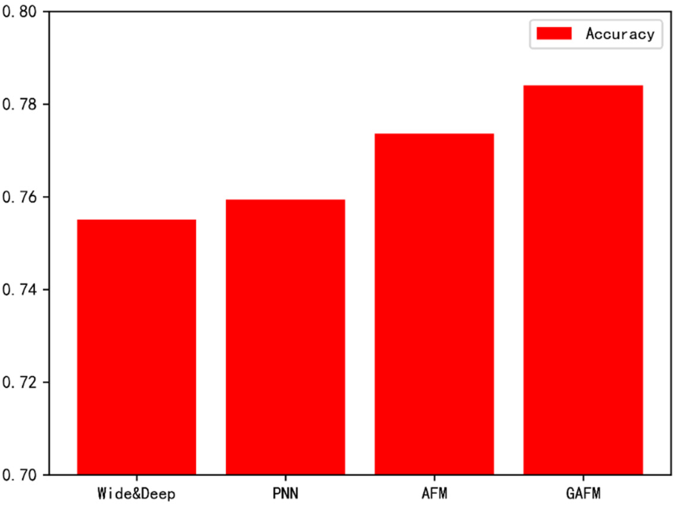
As can be seen from Figure 16, the performance of GAFM model on dataset 1 is significantly better than that of existing models.
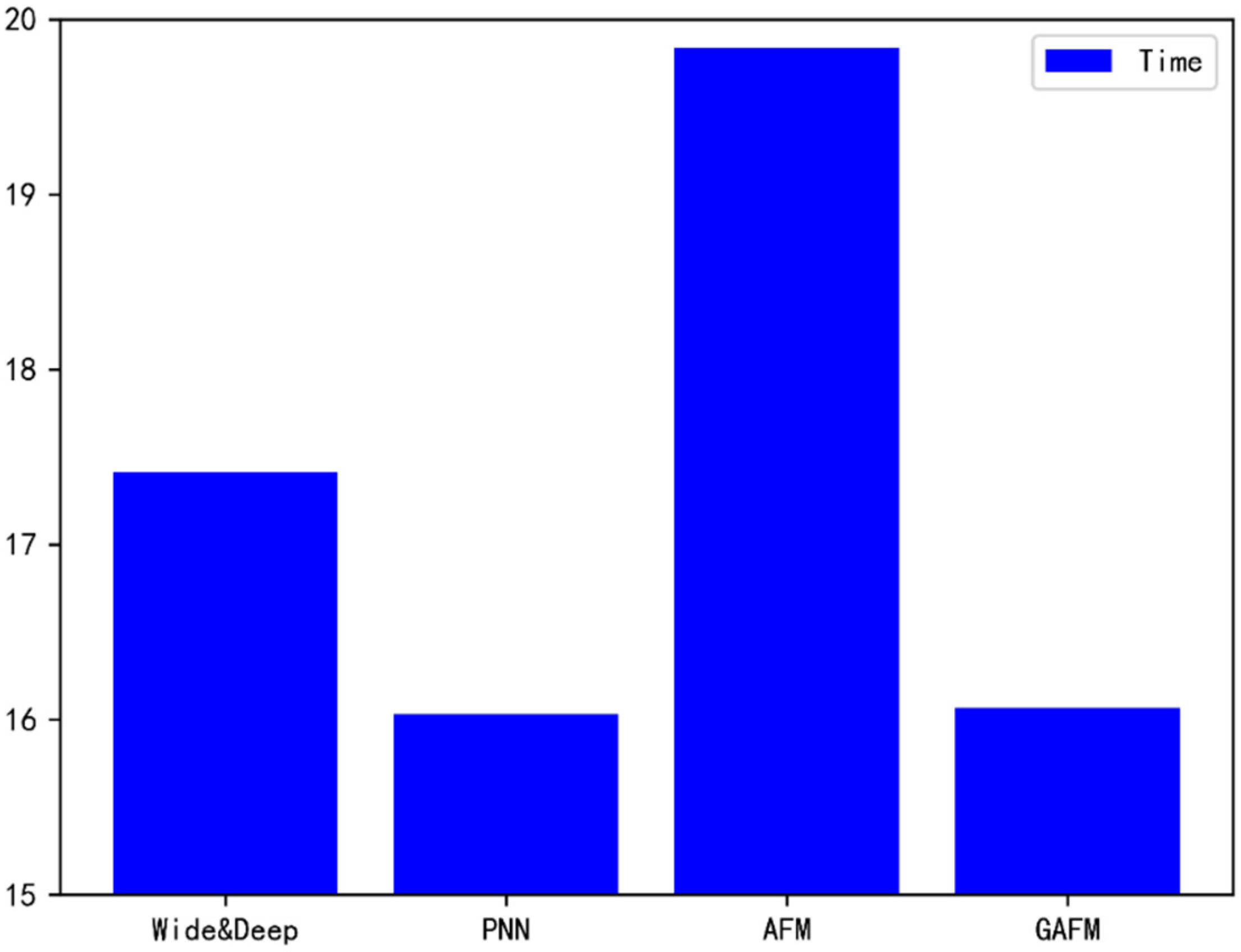
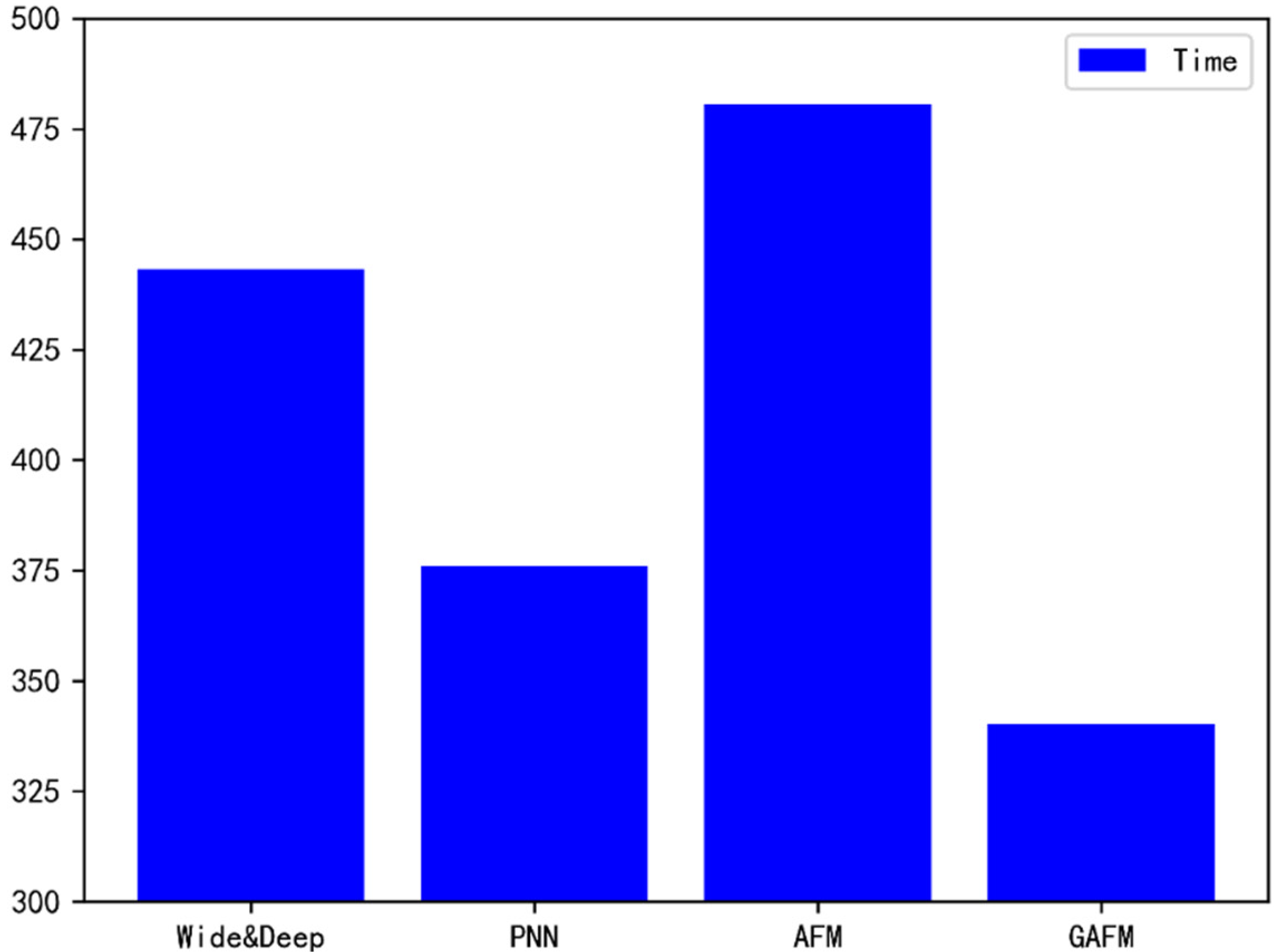
As can be seen from Figure 17, the running time of GAFM model on dataset 1 is significantly less than that of Wide & Deep model and AFM model, which is similar to that of PNN model.
(2) Dataset 2 is the experimental effect on the 1 M Movielens dataset:
As can be seen from Figure 18, similarly, the GAFM model performs well in accuracy.
It is obvious from Figure 19 that compared with dataset 1, the running time of GAFM on dataset 2 is significantly less than that of other models, which has obvious advantage.
(3) The experimental effect on dataset 3, namely the Movielens dataset with the size of 10 M:
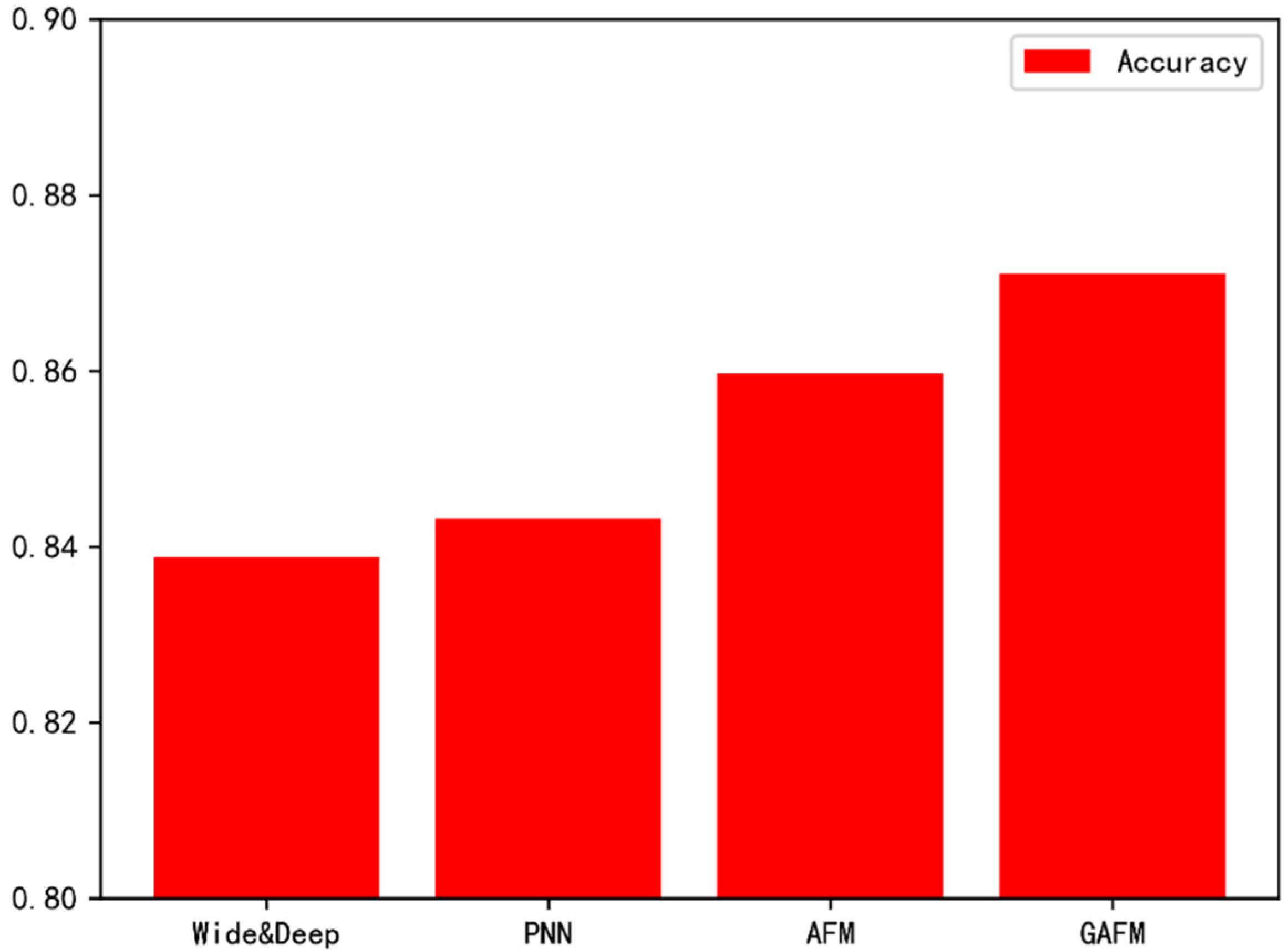
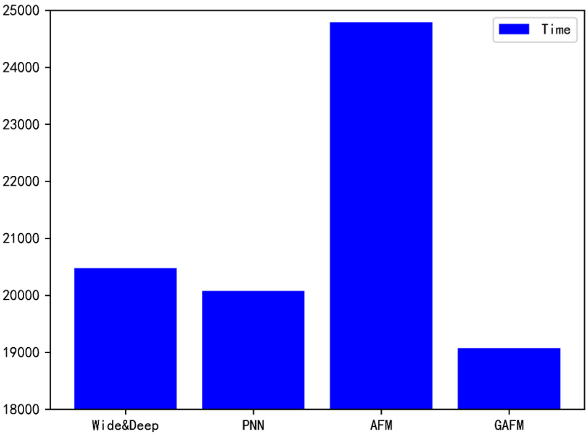
We can draw a basic conclusion from Figure 20 and Figure 21 that GAFM has more and more obvious advantages in accuracy and time with the increase of dataset size.
(4) Performance growth:
Annotation. The improvments part is the growth of accuracy and the growth of speed.
It can be concluded from Table 2 that GAFM’s time optimization is particularly obvious in the two factors of accuracy and time, and GAFM has incomparable advantages compared with AFM which is obviously backward in running speed.
5. Discussion
As can be seen from the experimental results in the fourth part, the GAFM proposed in this paper has the dual advantages of prediction accuracy and speed on different data sets. Specifically, we have the following findings:
1. The influence of parameter drop on the accuracy and speed of model prediction is positive, but it will fluctuate to different degrees due to the size of data set, and the influence effect is not significant compared with that of parameter g, but as a component of GAFM, it can play a role in adjusting the structure of model effect.
2. The influence of parameter g on the accuracy and speed of the model is significant. With the increase of g, the prediction accuracy of the model increases while the running speed decreases, which can be used to select the best value of g. In this paper, g = 0.91 is selected, this will be explained later in this paper.
3. According to the experimental results, when the value of parameter g is low, it does not have a good effect in terms of accuracy. Even though it is fast in speed, it should be abandoned in practical application. Only when g is greater than a threshold value the comparison of accuracy can have practical significance.
4. GAFM model on the data sets of different size is different, the significance of a comparison of three data sets, the greater the size of the data set and adjust the parameter g for the more significant the influence of running speed, and time factors on small data sets is very small, so the GAFM is suitable for the large data feature engineering scenarios recommendation system, can significantly optimize the accuracy and speed.
In this paper, the three models compared with GAFM are Wide & Deep, PNN and AFM. Except for the low accuracy when g value is too low, GAFM is better than Wide & Deep model in both accuracy and speed, while the accuracy is better than PNN when g value is high and the speed is similar. When g value is low, the speed is obviously better than AFM and the accuracy is similar. Therefore, in the actual application scenario, it is necessary to adjust the values of parameters g and drop repeatedly to reach an optimal solution suitable for this scenario, which is crucial for the overall efficiency of the model, scenarios in this experiment, comprehensive consider three data sets, because the parameter g for accuracy and running speed, especially with high sensitivity, selection and parameter value too low will lead to sharply lower accuracy, through the test, the drop = 0.84 selecting parameters, parameter g = 0.91, can achieve the optimal effect on the three data sets, and it’s a nice improvement over other models. Overall, GAFM improves both prediction accuracy and operating speed.
6. Conclusions and Future Work
Starting from solving the balance between accuracy and time of the recommendation system model, this paper explores various factors affecting the complexity of the model, innovatively adds the “gate” structure on the basis of the framework of the Wide & Deep series model, and proposes the GAFM model, which has achieved considerable results. Specifically, we divided the factors affecting the model complexity into data complexity and model structure complexity, and added the methods to solve the two kinds of problems into the two “gates”, respectively, adjusting the data scale and model structure, and achieving the balance between prediction accuracy and speed. We put our model on three data sets of different sizes and scenarios for horizontal comparison test, and the final experiment proved that compared with the existing model, GAFM model has significant advantages in both accuracy and speed.
In the future work, we hope to realize automatic learning of the model to find the optimal parameter g to adapt to different application scenarios, because it is troublesome to adjust the parameters repeatedly and it may not be able to find the best results, so automatic learning is a very necessary technology, which may need to rely on the relevant knowledge of reinforcement learning. Secondly, we plan to optimize the model structure of GAFM so that it can be significantly better than PNN model in time and AFM model in accuracy, making GAFM more convincing in a variety of application scenarios. Finally, we will continue to explore other potential factors affecting the complexity of the model, and discuss its reliability, whether it fits the GAFM model, and if it does, we will find ways to add it to the existing model to further improve the efficiency of the model.
Author Contributions
Conceptualization, H.Y.; methodology, H.Y.; software, H.Y.; validation, H.Y.; formal analysis, H.Y.; writing—original draft preparation, H.Y.; writing—review and editing, Y.L.; supervision, J.Y. All authors have read and agreed to the published version of the manuscript.
Funding
This research was funded by the National Natural Science Foundation of China under Grant 61971268 and the MOE (Ministry of Education in China) Project of Humanities and Social Sciences (Project No.19YJC760049).
Institutional Review Board Statement
Not applicable.
Informed Consent Statement
Not applicable.
Data Availability Statement
The datasets in this study are available online at UCI Machine Learning Repository: Adult Data Set and MovieLens|GroupLens.
Acknowledgments
We thank the National Natural Science Foundation of China for funding our work, grant number 61971268 and the MOE (Ministry of Education in China) Project of Humanities and Social Sciences (Project No.19YJC760049).
Conflicts of Interest
The authors declare no conflict of interest.
Abbreviations
The following abbreviations are used in this manuscript:
| PNN | Product-based Neural Network |
| CNN | Convolutional Neural Network |
| RNN | Recurrent Neural Network |
| FNN | Factorization Neural Network |
| FM | Factorization Machine |
| Deep | FM Deep Factorization Machine |
| NFM | Neural Factorization Machine |
| AFM | Attentional Factorization Machine |
| RELU | Rectified Linear Unit |
References
- Genius TV. An Integrated Approach to TV & VOD Recommendations; Archived 6 June 2012 at the Wayback Machine; Red Bee Media: London, UK, 2012. [Google Scholar]
- Liu, H.; Kong, X.; Bai, X.; Wang, W.; Bekele, T.M.; Xia, F. Context-Based Collaborative Filtering for Citation Recommendation. IEEE Access 2015, 3, 1695–1703. [Google Scholar] [CrossRef]
- Wu, Y.; Wei, J.; Yin, J.; Liu, X.; Zhang, J. Deep Collaborative Filtering Based on Outer Product. IEEE Access 2020, 8, 85567–85574. [Google Scholar] [CrossRef]
- Shan, H.; Banerjee, A. Generalized probabilistic matrix factorizations for collaborative filtering. In Proceedings of the IEEE International Conference on Data Mining, Sydney, Australia, 13–17 December 2010; pp. 1025–1030. [Google Scholar]
- Luo, X.; Zhou, M.; Xia, Y.; Zhu, Q. An efficient non-negative Matrix Factorization-Based approach to collaborative filtering for recommender systems. IEEE Trans. Ind. Inform. 2014, 10, 1273–1284. [Google Scholar]
- Wright, R.E. Logistic Regression. In Reading and Understanding Multivariate Statistics; Grimm, L.G., Yarnold, P.R., Eds.; American Psychological Association: Washington, DC, USA, 1995; pp. 217–244. [Google Scholar]
- Zheng, Z.; Yang, Y.; Niu, X.; Dai, H.; Zhou, Y. Wide and Deep Convolutional Neural Networks for Electricity-Theft Detection to Secure Smart Grids. IEEE Trans. Ind. Inform. 2018, 14, 1606–1615. [Google Scholar] [CrossRef]
- Vedaldi, A.; Lenc, K. Matconvnet: Convolutional neural networks for matlab. In Proceedings of the 23rd ACM International Conference on Multimedia, Brisbane, Australia, 26–30 October 2015; pp. 689–692. [Google Scholar]
- Mikolov, T.; Karafiát, M.; Burget, L.; Cernocký, J.; Khudanpur, S. Recurrent neural network based language model. In Proceedings of the Eleventh Annual Conference of the International Speech Communication Association, Chiba, Japan, 26–30 September 2010. [Google Scholar]
- Luft, J.H. Improvements in epoxy resin embedding methods. J. Biophys. Biochem. Cytol. 1961, 9, 409–414. [Google Scholar] [CrossRef] [PubMed]
- Zhang, W.; Du, T.; Wang, J. Deep Learning over Multi-Field Categorical Data. In European Conference on Information Retrieval; Springer: Cham, Switzerland, 2016; pp. 45–57. [Google Scholar]
- Goldberg, D.; Nichols, D.; Oki, B.M.; Terry, D. Using collaborative filtering to weave an information tapestry. Commun. ACM 1992, 35, 61–70. [Google Scholar] [CrossRef]
- Linden, G.; Smith, B.; York, J. Amazon.com recommendations: Item-to-item collaborative filtering. IEEE Internet Comput. 2003, 7, 76–80. [Google Scholar] [CrossRef] [Green Version]
- Koren, Y.; Bell, R.; Volinsky, C. Matrix factorization techniques for recommender systems. Computer 2009, 42, 30–37. [Google Scholar] [CrossRef]
- Rendle, S. Factorization machines. In Proceedings of the 2010 IEEE International Conference on Data Mining, Sydney, Australia, 13–17 December 2010; pp. 995–1000. [Google Scholar]
- Sedhain, S.; Menon, A.K.; Sanner, S.; Xie, L. Autorec: Autoencoders meet collaborative filtering. In Proceedings of the 24th International Conference on World Wide Web, Florence, Italy, 18–22 May 2015; pp. 111–112. [Google Scholar]
- Shan, Y.; Hoens, T.R.; Jiao, J.; Wang, H.; Yu, D.; Mao, J.C. Deep crossing: Web-scale modeling without manually crafted combinatorial features. In Proceedings of the 22nd ACM SIGKDD International Conference on Knowledge Discovery and Data Mining, San Francisco, CA, USA, 13–17 August 2016; pp. 255–262. [Google Scholar]
- He, X.; Liao, L.; Zhang, H.; Nie, L.; Hu, X.; Chua, T.S. Neural collaborative filtering. In Proceedings of the 26th International Conference on World Wide Web, Perth, Australia, 3–7 April 2017; pp. 173–182. [Google Scholar]
- Qu, Y.; Cai, H.; Ren, K.; Zhang, W.; Yu, Y.; Wen, Y.; Wang, J. Product-based neural networks for user response prediction. In Proceedings of the 2016 IEEE 16th International Conference on Data Mining (ICDM), Barcelona, Spain, 12–15 December 2016; pp. 1149–1154. [Google Scholar]
- Cheng, H.T.; Koc, L.; Harmsen, J.; Shaked, T.; Chandra, T.; Aradhye, H.; Anderson, G.; Corrado, G.; Chai, W.; Ispir, M.; et al. Wide & deep learning for recommender systems. In Proceedings of the 1st Workshop on Deep Learning for Recommender Systems, Boston, MA, USA, 15 September 2016; pp. 7–10. [Google Scholar]
- Guo, H.; Tang, R.; Ye, Y.; Li, Z.; He, X. DeepFM: A factorization-machine based neural network for CTR prediction. arXiv 2017, arXiv:1703.04247. [Google Scholar]
- He, X.; Chua, T.S. Neural factorization machines for sparse predictive analytics. In Proceedings of the 40th International ACM SIGIR Conference on Research and Development in Information Retrieval, Tokyo, Japan, 7–11 August 2017; pp. 355–364. [Google Scholar]
- Xiao, J.; Ye, H.; He, X.; Zhang, H.; Wu, F.; Chua, T.S. Attentional factorization machines: Learning the weight of feature interactions via attention networks. arXiv 2017, arXiv:1708.04617. [Google Scholar]
- Sunil Ray. 8 Proven Ways for improving the “Accuracy” of a Machine Learning Model. Anal. Vidhya 2015, 12. Available online: https://www.analyticsvidhya.com/blog/2015/12/improve-machine-learning-results/ (accessed on 11 October 2021).
- Van Smeden, M.; Moons, K.G.; de Groot, J.A.; Collins, G.S.; Altman, D.G.; Eijkemans, M.J.; Reitsmana, J.B. Sample Size for Binary Logistic Prediction Models: Beyond Events Per Variable Criteria. Stat. Methods Med Res. 2019, 28, 2455–2474. [Google Scholar] [CrossRef] [PubMed] [Green Version]
- Juba, B.; Le, H.S. Precision-Recall versus Accuracy and the Role of Large Data Sets; Association for the Advancement of Artificial Intelligence: Palo Alto, CA, USA, 2018. [Google Scholar]
- Lei, S.; Zhang, H.; Wang, K.; Su, Z. How Training Data Affect the Accuracy and Robustness of Neural Networks for Image Classification. In Proceedings of the International Conference on Learning Representations, New Orleans, LA, USA, 6–13 May 2019. [Google Scholar]
- Kohavi, R.; Becker, B. UCI Machine Learning Repository: Adult Data Set [EB/OL]. (1996-05-01). Available online: https://archive.ics.uci.edu/ml/datasets/adult (accessed on 17 February 2005).
- Harper, F.M.; Konstan, J.A. The MovieLens Datasets: History and Context. ACM Trans. Interact. Intell. Syst. 2015, 5, 1–19. [Google Scholar] [CrossRef]
Figure 1.
Main structure of GAFM.

Figure 2.
The difference between Dropout and Drop.

Figure 3.
The key currency principle of attention layer.

Figure 4.
Prediction accuracy of GAFM under the influence of the drop value.

Figure 5.
Prediction accuracy of GAFM under the influence of g value.

Figure 6.
Prediction accuracy of GAFM under drop.

Figure 7.
Prediction accuracy of GAFM under the influence of g.

Figure 8.
Prediction accuracy of GAFM under drop.

Figure 9.
Prediction accuracy of GAFM under the influence of g.

Figure 10.
Running time of GAFM under the influence of drop.

Figure 11.
Running time of GAFM under the influence of g.

Figure 12.
Running time of GAFM under the influence of drop.

Figure 13.
Running time of GAFM under the influence of g.

Figure 14.
Running time of GAFM under the influence of drop.

Figure 15.
Running time of GAFM under the influence of g.

Figure 16.
The accuracy of each model is compared.

Figure 17.
The running time of each model is compared.

Figure 18.
The accuracy of each model is compared.

Figure 19.
The running time of each model is compared.

Figure 20.
The accuracy of each model is compared.

Figure 21.
The running time of each model is compared.


Table 1.
Factors that affect accuracy and speed.
| Complexity of Model | Complexity of Data | Embedding | Regularization | Weight Calculation | |
|---|---|---|---|---|---|
| accuracy | |||||
| speed |
Annotation. means Positive correlation, means Negative correlation.
Table 2.
Performance growth of GAFM compared to other models.
| Baselines | Improvements |
|---|---|
| Wide & Deep | +2.76%&& + 7.58% |
| PNN | +2.44%&& + 4.93% |
| AFM | +1.17%&& + 24.09% |
Publisher’s Note: MDPI stays neutral with regard to jurisdictional claims in published maps and institutional affiliations. |
© 2021 by the authors. Licensee MDPI, Basel, Switzerland. This article is an open access article distributed under the terms and conditions of the Creative Commons Attribution (CC BY) license (https://creativecommons.org/licenses/by/4.0/).
Share and Cite
MDPI and ACS Style
Yu, H.; Yin, J.; Li, Y. Gate Attentional Factorization Machines: An Efficient Neural Network Considering Both Accuracy and Speed. Appl. Sci. 2021, 11, 9546. https://0-doi-org.brum.beds.ac.uk/10.3390/app11209546
AMA Style
Yu H, Yin J, Li Y. Gate Attentional Factorization Machines: An Efficient Neural Network Considering Both Accuracy and Speed. Applied Sciences. 2021; 11(20):9546. https://0-doi-org.brum.beds.ac.uk/10.3390/app11209546
Chicago/Turabian StyleYu, Huaidong, Jian Yin, and Yan Li. 2021. "Gate Attentional Factorization Machines: An Efficient Neural Network Considering Both Accuracy and Speed" Applied Sciences 11, no. 20: 9546. https://0-doi-org.brum.beds.ac.uk/10.3390/app11209546
Note that from the first issue of 2016, this journal uses article numbers instead of page numbers. See further details here.