Article

Experimental and Computational Aeroacoustic Investigation of Small Rotor Interactions in Hover

1
Department of Mechanical Engineering, Boston University, Boston, MA 02215, USA
2
Department of Engineering, Roma Tre University, 00146 Roma, Italy
*
Author to whom correspondence should be addressed.
Submission received: 4 October 2021 / Revised: 15 October 2021 / Accepted: 23 October 2021 / Published: 26 October 2021
(This article belongs to the Special Issue Aerodynamic Aeroelasticity and Aeroacoustics of Rotorcraft)

Abstract

:
This paper investigates the aeroacoustic interactions of small hovering rotors, using both experiments and computations. The experiments were conducted in an anechoic chamber with arrays of microphones setup to evaluate the azimuthal and polar directivity. The computational methodology consists of high fidelity detached eddy simulations coupled to the Ffowcs-Williams and Hawkings equation, supplemented by a trailing edge broadband noise code. The aerodynamics and aeroacoustics of a single rotor are investigated first. The simulations capture a Reynolds number effect seen in the performance parameters that results in the coefficient of thrust changing with the RPM. The acoustic analysis enables the identification of self-induced noise sources. Next, dual side-by-side rotors are studied in both counter-rotating and co-rotating configurations to quantify the impact of their interactions. Higher harmonics appear due to the interactions and it is verified that the counter-rotating case leads to more noise and a less uniform azimuthal directivity. Difficulties that arise when trying to validate small rotor calculations against experiments are discussed. Comparisons of computational and experimental results yield further insight into the noise mechanisms that are captured by each methodology.

1. Introduction

The rapid progress in the electric vertical takeoff and landing (eVTOL) industry warrants the need for fundamental understanding of flight-enabling technology. Aircraft from the scale of unmanned aerial vehicles (UAVs) for drone delivery to urban air mobility (UAM) transport vehicles rely on multiple rotors to attain controlled flight. These rotors will experience significant aerodynamic interactions that have implications on performance and noise. It is necessary to develop experimental and computational methods for the evaluation of these vehicles, whose noise could have implications on their acceptance in our society [1].
However, even the fundamental problem of a single rotor in hover poses an issue to the scientific community because of the difficulty in characterizing the noise sources. Experiments are contaminated by the influence of external factors, such as motor noise, interactions with test equipment, the influence of ground effect, recirculation in confined environments, and turbulence or gusts in open environments [2,3,4,5,6]. In addition, even when the effects of the environment are mitigated, the sources that contribute to both the tonal and broadband noise cannot be investigated without high resolution surface data or advanced flow visualization techniques, both of which are still in development. Computational approaches fulfill this need to study aeroacoustics in greater detail by providing insight into the flow physics and noise source localization [7,8]. Yet, it is challenging to incorporate all of the potential external factors from the experiments into computations; this calls into question whether validation is possible.
In lieu of validation, one can consider verification. However, even this is a bit complicated, with some in the field using Navier–Stokes (NS) codes that are based on the governing equations for fluid motion and others using Lattice–Boltzmann methods (LBM) based on kinetic equations to describe fluid motion. Each of these approaches is even further subdivided: for example, Navier–Stokes methods range in order of increasing turbulence resolution and cost from unsteady Reynolds-averaged Navier–Stokes (URANS) to large eddy simulation (LES) to direct numerical simulation (DNS) [9]. Due to the intense computational requirements of LES and DES methods, hybrid approaches, such as hybrid URANS/LES or detached eddy simulation (DES), have been popularized in which the turbulence is fully resolved when the turbulence length scales are greater than that of the CFD grid spacing. However, these approaches typically require a turbulence model near the wall, and model selection can also affect the results [10,11,12]. Similarly, the LBM modeler has to make choices in terms of their collision models, subgrid-scale turbulence models, and boundary conditions [13]. There is no unified approach for either LBM or NS that can be applied to every situation, due to computational constraints. Finally, for both LBM and NS methods, the user must also generate a mesh that is compatible with the chosen models and chosen geometry. Improper mesh generation is often the largest source of user error for CFD codes.
The resolution of turbulence and overall numerical accuracy in the entire domain dictates which computational aeroacoustics (CAA) methodology should be used, which noise sources are automatically captured, and the accuracy of the acoustic prediction. In this work, a DES is used to capture some of the turbulent spectrum; due to the nature of the grid, the pressure is only expected to be resolved well near the rotor surfaces. This scenario is well-suited for usage of the Ffowcs-Williams Hawking (FWH) analogy, which uses near-field velocity and pressure results to obtain the acoustics [14]. This methodology introduces additional issues of its own. For example, there is much debate over whether a permeable surface integration is superior to a simple impermeable, or solid, surface integration for small rotors [15]. The impermeable integration is applied on the rotor surface and describes both the thickness and loading noise, but neglects the quadrupole noise. On the other hand, the permeable surface is placed in the volume and is able to capture all of the noise sources. However, even when a user elects to use the permeable surface method, there is no common approach for its topology and placement. The surface must be placed close enough such that the effects of numerical dissipation are minimized but far enough to avoid hydrodynamic waves contaminating the acoustic waves, leading to spurious signals [16]. Finally, it is still unknown which combination of CFD and CAA approaches are able to capture the broadband noise, which can be caused by turbulence ingestion, wake interactions, or self noise [17,18]. Even the higher harmonic noise nominally associated with unsteady loading is seemingly sensitive to the methods.
In general, researchers have shown contradictory results both experimentally and computationally, indicating that the aeroacoustic characterization is extremely sensitive to the methodology. This paper describes experimental and computational findings for a single small rotor and small dual rotors in hover. These rotor configurations are not new. However, the exact rotor geometry was available from the manufacturer, allowing computational grids to be developed that represent well the rotor used in the experiment. In addition, the CFD suite of codes that are used was validated well for traditional large rotorcraft and was only recently applied to small rotors. What is presented in this paper, therefore, adds to the database of small rotor results that must continue to grow in order to enable the community to determine best practices for small rotor simulations.
To contextualize the current work, a summary of active research in the community is provided in the following background section, focusing on the three following topics: Section 2.1 highlights the significance of structural modeling and manufacturing discrepancies. Section 2.2 discusses the amplification of noise due to flow confinement. Section 2.3 compares results, using the impermeable and permeable surface, and also identifies the approaches to capturing broadband noise. Section 2.4 describes the efforts made to quantify aerodynamic interactions and their effects on noise.
Section 3.1 provides a description of the rotor configuration. The experimental setup for acoustics measurements at Roma Tre University is described in Section 3.2. The computational methodology involving the CFD and CAA tools used, including the computational mesh, is defined in Section 3.3. Next, the performance results are presented and discussed in Section 4.1 and the acoustics results are discussed in Section 4.2. The paper concludes with a summary of significant findings and potential future work in Section 5.

2. Background

In this section, we highlight results of others who have considered single and dual small rotors computationally and experimentally. The main goals of this section are to describe the known challenges and highlight the inconsistencies in the reported findings.

2.1. The Dependence on Rotor Materials and Manufacturing

Russell et al. studied multiple small rotors made of carbon fiber and injection molded plastic [19]. They showed that the injection molded plastic rotor is more susceptible to deflections. In addition, they tested five versions of the same rotor made of plastic and had a wide range of measured tip twist deflections across the entire RPM range tested. Both the manufacturing discrepancies and the blade material properties had an impact on the experimental results. In fact, they showed that incorporation of an elasticity model in the computations shows better agreement with the experimental measurements. However, this modification did not impact the thrust. Russell et al. also acknowledged the difficulty of defining the blade properties and had to iteratively adjust the material properties in the model based on the experimental results. The rotor structure is an important contributor to the performance and noise, but it is often difficult to quantify the effects in a way that can be integrated into the computations.

2.2. The Impact of Recirculation

Zawodny et al. conducted acoustic measurements of small-scale rotors in the NASA Langley Structural Acoustic Loads and Transition acoustic chamber and reported that the build up of recirculation resulted in high amplitude fluctuations in the load cell signals [20]. Weitsman et al. quantified the impacts of recirculation on rotor noise in closed anechoic chambers by examining the spectrogram of the acoustic pressure signal at several mic locations [4]. They showed that, after the flow develops in the chamber, not only does the thrust signal fluctuate wildly, but both the higher harmonic noise and broadband noise are amplified. This discovery somewhat conflicts with traditional acoustic measurement techniques in which the rotor is run at a constant operating condition until either the performance values or the acoustic signal reaches a steady state before data are collected. Therefore, care must be taken to record measurements prior to the effect of recirculation and after the rotor loads have stabilized. This window of opportunity can be very small depending on the rotor geometry, test equipment, and chamber size. They found that placing woven screen meshes in the wake could delay the effect of recirculation and enable a longer measurement duration. Whelchel et al. similarly made attempts to mitigate the effects of recirculation using a similar mesh screen, but their results were inconclusive [5], emphasizing the difficulties in conducting aeroacoustics experiments.
Nardari et al. were able to highlight the effect of recirculation [21]. They developed an experimental approach that ensured recirculation by maintaining the hovering operating condition until the aerodynamic loads were steady. They used the LBM solver PowerFLOW to simulate a confined and unconfined environment for a single rotor. They then showed that the confined simulation showed much better agreement than the unconfined simulation, especially at higher harmonics. They were able to examine the noise-generation mechanisms and identify leading-edge interactions with the recirculated vortices that amplified the higher harmonic peaks. However, the broadband components of the sound power watt level (PWL) of the confined and unconfined simulations were nearly identical. In addition, although neither the rotor rotation rate nor the absolute sound levels were reported, the PWL of the simulations underpredicted the experimental values by approximately 5 dBA/Hz.

2.3. The Difficulties of Acoustic Predictions

Casalino et al. implemented the LBM model in the PowerFLOW solver to simulate a low Reynolds number propeller at various advance ratios and obtained excellent agreement with experiments for hover, capturing both tonal and broadband noise [8]. They used both solid and permeable surface integration methods and showed that the integration surface had minimal impact on the results, indicating that the quadrupole effect was small and noise sources could be localized on the surface. This is in agreement with work by previous researchers that showed that the quadrupole noise scaled with the Mach number, and thus should be low for these small rotors.
However, Mankbadi et al. also performed simulations of a UAV propeller using a hybrid URANS/LES approach and found that a permeable surface integration showed great agreement with experimental data, but an impermeable surface integration could not capture the higher harmonic tones nor the broadband [7]. Mankbadi et al. attributed the difference between the permeable and impermeable surface results to noise sources present in the wake. However, the contribution of these sources is higher than one expects for quadrupole terms.
Finally, the presence of higher harmonic noise in experimental measurements is attributed to either recirculation [4] or unsteady motor variations [22]. Often, these harmonics do not appear in computational results, especially those that use low-fidelity blade element theory models [3,8,23,24,25]. However, some computational works that do not model recirculation or rotation rate perturbations also predict higher harmonics that seem to coincide with measured values [7,8,26].

2.4. The Significance of Rotor Interactions

Precise quantification of the impact of rotor interactions is necessary to inform conceptual design choices. Aircraft designers must limit the overall size of their vehicles but also ensure that their rotors are operating with high efficiency. Zhou et al. performed experiments of small hovering rotors and used stereoscopic particle image velocimetry (PIV) to capture the induced interactional flow [27]. They found increased tonal and broadband noise with increasing rotor proximity, characterized by enhanced turbulent kinetic energy in the gap region. They found that, although the mean thrust was the same, the thrust fluctuations increased with proximity as well. Shukla et al. similarly conducted PIV measurements of side-by-side rotors and also found that increased rotor proximity leads to increased wake interactions, although acoustic measurements were not performed and the performance results were inconclusive [28].
Some medium fidelity CFD simulations have captured reasonable interactional acoustics trends. For example, Lee et al. used the nonlinear vortex lattice method in combination with the vortex particle method (VPM) to predict the noise of a quadrotor and showed a decrease in noise with rotor separation distance [29]. Bernardini et al. used a boundary element method (BEM) to characterize the aeroacoustic signature of propeller arrays [30]. They found that the interactional noise caused by twin rotors greatly affected the directivity of the overall noise, with noise increases up to 50 dB, much greater than a simple pressure doubling. Broadband noise was not considered, and the findings were not backed up by experimental results.
Alvarez et al. compared URANS and the vortex particle method (VPM) approaches to rotor-on-rotor aerodynamics [24]. However, they used rather coarse time steps for their URANS simulations and used a compact source approximation for the acoustics. They were able to capture the first blade passage frequency (BPF) tone of the isolated rotor simulations well, but were unable to predict the increase in the higher harmonic tonal noise from the experiments in their URANS simulations. They did not include their high-fidelity broadband spectrum in their paper. On the other hand, Afari et al. conducted hybrid URANS/LES simulations of inline counter-rotating propellers in hover and discovered a large increase in the broadband noise, compared to the single rotor and negligible change in the higher harmonics [31]. Again, experimental measurements were not available for comparison. There has also been extensive computational work studying the NASA eVTOL common reference models, but the experimental characterization of these models was not conducted [32,33,34,35].
In this research, a DES, a type of hybrid URANS/LES method, is used to further investigate aerodynamic interactions and their impact on noise. Accompanying experimental data are used for comparison. Isolated rotor measurements and simulations are conducted to capture the aerodynamics and aeroacoustics of a single rotor at various rotor speeds. Then, a single RPM is chosen and used to investigate dual rotors in both co-rotating and counter-rotating configurations. Their tip-to-tip spacing is gradually increased to explore the impact of their interactions on both performance and noise.

3. Materials and Methods

3.1. Rotor Configuration

The rotor geometry chosen for this study is the advanced precision composite (APC) 8x45MR rotor, referred to in this paper as APC8x45MR. The name distinguishes the rotor diameter of 8 inches with a pitch of 4.5 inches, which was designed for multi-rotor (MR) configurations. Some other geometry details provided by APC include the hub diameter of 0.65 inches, a hub thickness of 0.33 inches, and a product weight of 0.32 ounces. This propeller is made of plastic using injection molding, and therefore may be subject to manufacturing defects that could impact the performance and noise. The computational model of the rotor was derived from the exact computer-aided design (CAD) geometry provided by APC for this study and will be discussed further in the Computational Methodology section. The counter-clockwise version of the rotor will be investigated for the isolated rotor and co-rotating dual rotor configurations. The counter-rotating dual rotor configuration includes one clockwise rotor and one counter-clockwise rotor.

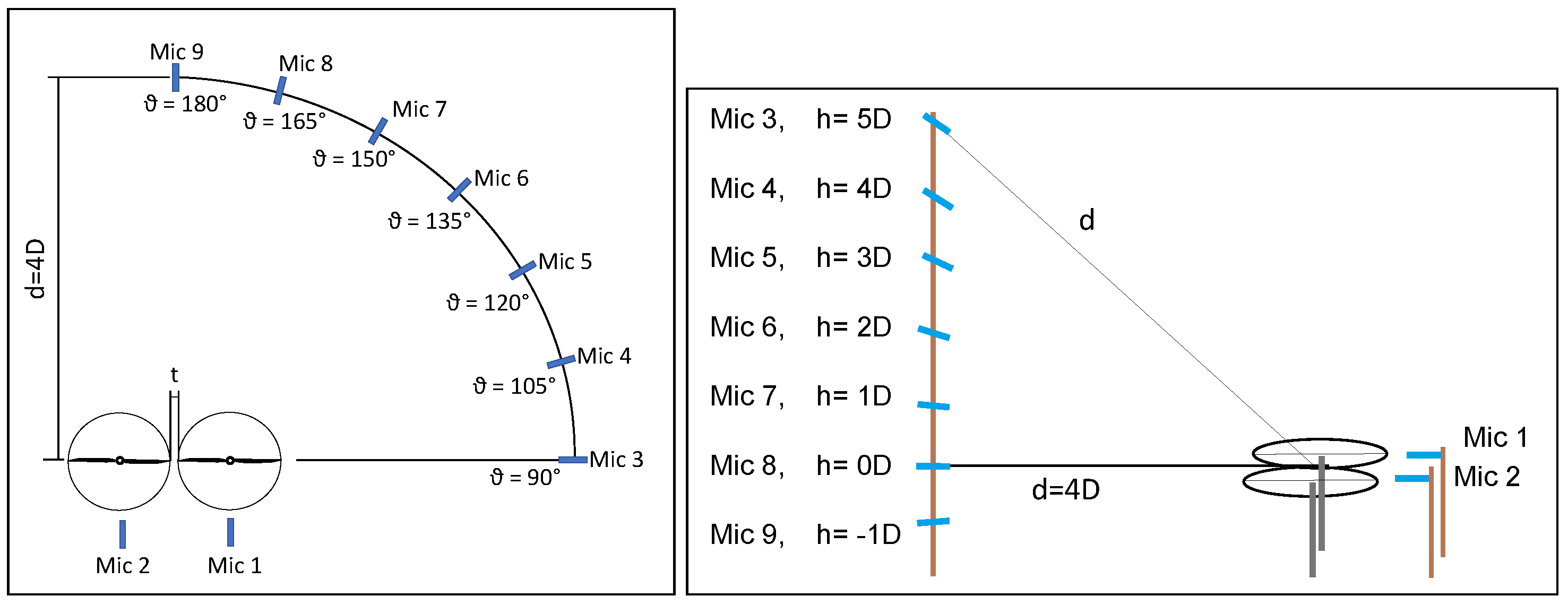
3.2. Experimental Setup

The experiments were conducted in the anechoic chamber of the Roma Tre University “G. Guj” fluid dynamics laboratory, which measures 3 m in height, 2 m in width and 4 m in length. The facility is treated with sound absorbent panels, and is able to absorb 99% of incident sound energy above 500 Hz. Due to the expected recirculation and turbulence ingestion effects, the flow was facilitated through an outlet. Each rotor was mounted in pusher configuration on a cylindrical support so that the propeller disk was at a height of 4 radii from the floor. A total of nine Microtech Gefell M360 free-field microphones were used to measure the pressure fluctuations from the rotors and characterize both azimuthal and polar directivity, using two different set-ups as shown in Figure 1.
The circular array was aligned with the rotor plane, and the microphones were located along a 90° arc at a distance of 8 rotor radii from the propeller hub center. The linear array was mounted parallel to the test stand at a radial distance of 8 rotor radii from the hub center, with the microphones spaced by 2 rotor radii and directed toward the center of the rotor system. Two more microphones were placed in the nearfield of the rotors at a distance that was determined to not influence the flow evolution. These microphones were used to control the rotational speeds of the rotors.
A LabView program was used for the open loop control of the propellers and to collect the data. The acoustic signals were acquired simultaneously for 5 s at a sampling rate of 100 kHz, using a NI PXI-6143 data acquisition unit installed on a NI PXIe-8840 chassis. Isolated and twin rotor configurations were tested by varying the rotational speed, the sense of rotation and the tip-to-tip clearance.
Additional information can be found in De Paola’s PhD thesis [6].

3.3. Computational Methodology

Descriptions of the rotorcraft simulation suite used for the CFD, the aeroacoustics solver used for the CAA, the broadband modeling framework, and the rotor geometry modeled for the simulations are presented in this section.

3.3.1. CREATE-AV Helios

The simulation framework used for the CFD portion of this study is the Department of Defense (DoD) High Performance Computing Modernization Program (HPCMP) code, CREATE-AV Helios version 11.0 [36,37,38]. Helios is an overset code developed by the U.S. Army Technology Development Directorate specifically for rotorcraft. Although it was originally used for helicopters, it was recently validated for small rotorcraft on the scale of drones and UAVs [12,23,39,40]. For this work, the Reynolds-averaged Navier–Stokes (RANS) equations are solved in the inertial frame, using the off-body solver SAMCART coupled to the near-body solver mStrand. A rendering of the overset mesh system near the blade tip is shown in Figure 2. A detached eddy simulation (DES) approach was used for the simulations in this study; therefore, the turbulent scales are resolved using LES when the grid is sufficient, and URANS is used otherwise [9].
SAMCART is a Cartesian grid solver that implements a 5th order central difference scheme with 4th order viscous terms for its spatial discretization and 2nd order backward differentiation in time. mStrand is a multi-strand finite volume solver that automatically generates the volume mesh during runtime, based on the surface discretization. mStrand uses a vertex centered approach with 2nd order spatial terms, and similarly uses 2nd order backward differentiation in time [41,42]. Other researchers have used NASA’s OVERFLOW for the near body, which is capable of using a 5th order spatial scheme with 2nd order discretization for the viscous terms [10,11,32,33,35,43,44,45,46,47,48,49]. However, the mesh generation procedure for OVERFLOW is more complicated than that of mStrand, which automatically generates the volume mesh [50]. Therefore, there is a trade-off, and we have selected mStrand for this study. The domain connectivity is handled by PUNDIT, described in further detail by Sitaraman et al. [51]. The Spalart–Allmaras (SA) turbulence model was chosen for this study, due to its robustness and accuracy, and is implemented in both the near body and off body [52]. Although laminar-turbulent transition models have been shown to improve torque predictions for low Reynolds number rotors, they are not used because they were also shown to lead to poor thrust predictions and increased computational cost [12].
The simulations were set up to match the isolated rotor, co-rotating dual rotor, and counter-rotating dual rotor configurations of the experiments. For all of the simulations, a time step of 0.25° azimuth was selected, corresponding to 1440 time steps per rotor revolution, based on prior rotorcraft CFD research [12,39,42,53]. Adaptive mesh refinement (AMR) was turned on in the off-body solver after two rotor revolutions. A total of 10 rotor revolutions were simulated, with the first 5 being used to allow the starting vortex to propagate away and properly develop the inflow. The acoustic calculations were then based on the last five. The results of simulations conducted in the present work will be referred to as the Helios results.

3.3.2. PSU-WOPWOP

The noise generated by an isolated rotor in a quiescent field can be computed based on the rotor’s surface pressure distribution and the rotor’s rotation rate. PSU-WOPWOP solves the Ffowcs-Williams Hawking (FWH) equation, using Farassat formulation 1A [54,55,56]. The thickness and loading acoustic pressure components are listed below as shown in [56]:
4 π p T ( x , t ) = f = 0 ρ 0 ( v ˙ n + v n ˙ ) r ( 1 M r ) 2 ret d S + f = 0 ρ 0 v n ( r M ˙ r + c M r c M 2 ) r 2 | 1 M r | 3 ret d S ,
4 π p L ( x , t ) = 1 c f = 0 l ˙ r r | 1 M r | 2 ret d S + f = 0 l r l M r | 1 M r | 2 ret d S + 1 c f = 0 l r ( r M ˙ r + c M r c M 2 ) r 2 | 1 M r | 3 ret d S .
Here, p T is the acoustic thickness pressure, p L is the acoustic loading pressure, c is the speed of sound in the fluid medium, ρ 0 is the fluid density, v n is the body’s normal velocity component, r ^ i is the radiation vector, r is the distance between the source and observer, l i = Δ P i j n ^ j is the surface loading vector, M i is the vectorized Mach number, and M r is the radiation Mach number. The terms l r and l M are the dot product of the loading vector with the radiation vector and vectorized Mach number, respectively. Although this formulation is used for both impermeable and permeable surface calculations, it should be noted that the Mach number terms are zero for the non-moving permeable surface, reducing the acoustic equation to three integrals.
The integrals are computed over the surfaces represented by f = 0 at the discrete elements of the computational mesh. The blade surface pressure and position were stored over the last five rotor revolutions for impermeable surface calculation. For the permeable surface, point probes were extracted from Helios’ off-body solver SAMCART to recreate the topology of a cylinder with radius 1.125R and length of 0.25R encapsulating the rotor. The bottom surface of the cylinder, in the rotor wake, was excluded to avoid hydrodynamic waves from the vortices contaminating the signal. A surface spacing of 0.025c was chosen to match the off-body fixed refinement region and minimize numerical interpolation errors. The coupling of the CFD and CAA methodology in this paper will be referred to as Helios/PSU-WOPWOP.

3.3.3. UCD-Quietfly

The broadband noise prediction framework UCD-Quietfly v1.0 developed by Li et al. [57,58,59] is used in this paper. The user inputs sectional airfoil geometry, velocity, and angle of attack, and the program automatically computes the boundary layer flow parameters, using XFOIL.
The noise of the unstalled sections is computed, using Lee’s wall pressure spectrum model [60] and the trailing-edge noise model by Amiet [61]. A correction to the implementation of Amiet’s model inside UCD-Quietfly is made in this paper to account for very small chord lengths. This correction, which was originally proposed by Moreau et al., effectively doubles the scattered pressure field by Amiet and results in a 6 dB increase in the sound pressure level (SPL) [62]. This modification is accounted for in newer versions of UCD-Quietfly starting with v2.0. The reader is referred to Lee et al. for a review of the turbulent boundary layer trailing-edge noise research [63].
Within UCD-Quietfly, the stalled airfoil sections are computed, using the Brooks, Pope, and Marcolini (BPM) model. The bluntness formulation of the BPM model may also be applied, but is typically negligible for small rotors. One supplies to UCD-Quietfly the sectional inflow and angle of attack. We use the high-fidelity CFD results to inform the inputs for this work. The tangential velocity component was taken as the relative rotation rate at the blade section, while the perpendicular velocity was taken from instantaneous point probes at the last timestep of the isolated rotor simulation placed 0.1D above the rotor plane along the rotor centerline. These velocities were combined with the sectional twist to compute the effective angles of attack. The airfoil at the 75% span location was used to calculate the boundary layer parameters, extracted at 99% chord in XFOIL, for the entire blade.

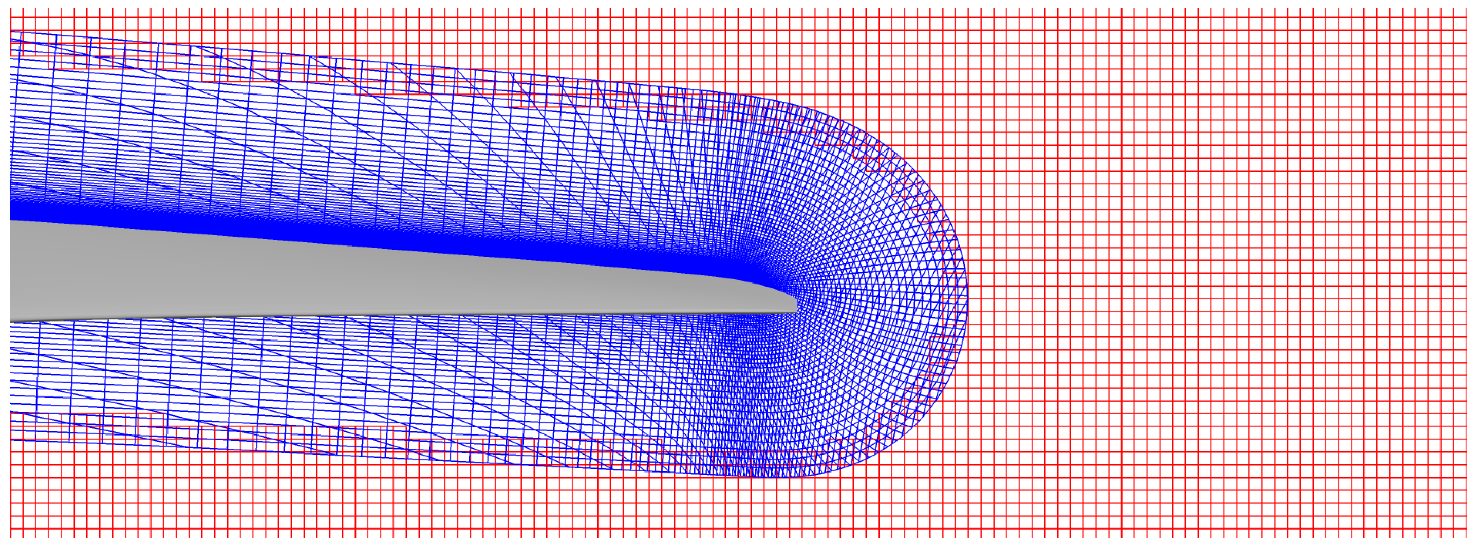
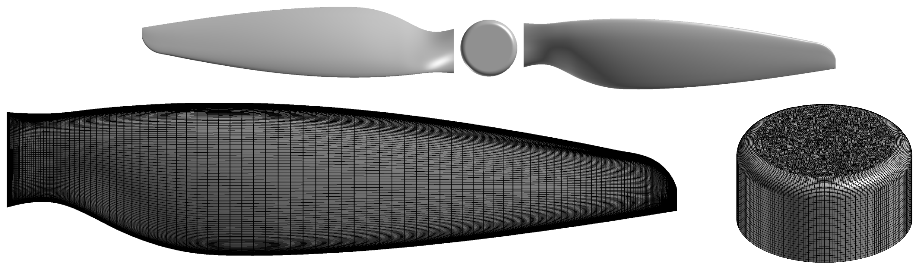
3.3.4. Rotor Geometry and Mesh

The CAD geometry of the APC8x45MR rotor was provided by APC and imported into Pointwise for surface mesh generation. The hub was modeled separately from the blades to avoid complex mesh generation at their intersection. The gap between the hub and the rotors was not expected to have a significant impact on the calculations due to the relatively low induced velocity inboard. However, the hub was included to mitigate the effects of artificially generated hub vortex caused by the separation. A picture of the computational model, including separate images for the rotor mesh and hub mesh, can be seen in Figure 3.
The rotor mesh was generated with 202 points along the span and 250 points around the airfoil. The root cutout was located at 0.1 R , and the tip was cut off at 0.99375 R . However, even though the tip was slightly trimmed, the rotor radius was still assumed to be 4 in. for the purpose of computing the performance coefficients and tip-tip distances. The wall spacing was computed to ensure y + < 1 and set to 10 4 c , where c is the mean chord. The strand length was set to 0.4 c and contains 51 points. The wake spacing of the near-body volume mesh was set to 0.025 c . A fixed refinement region of equal spacing was placed in the off-body volume mesh for proper interpolation of the solution between mStrand and SAMCart. These grid settings were determined to be sufficient for small scale rotors by Thai et al. [12].
The motors, load cells, test stand, and spinners were not included in the computational model but are not expected to significantly impact the aerodynamics. However, they may impact the acoustic measurements. In addition, the ground and surrounding walls were also not included, even though the recirculation effects may increase the noise as shown by Weitsman et al. [4] and Nardari et al. [21]. The limitation of this modeling approach is further discussed in the results.

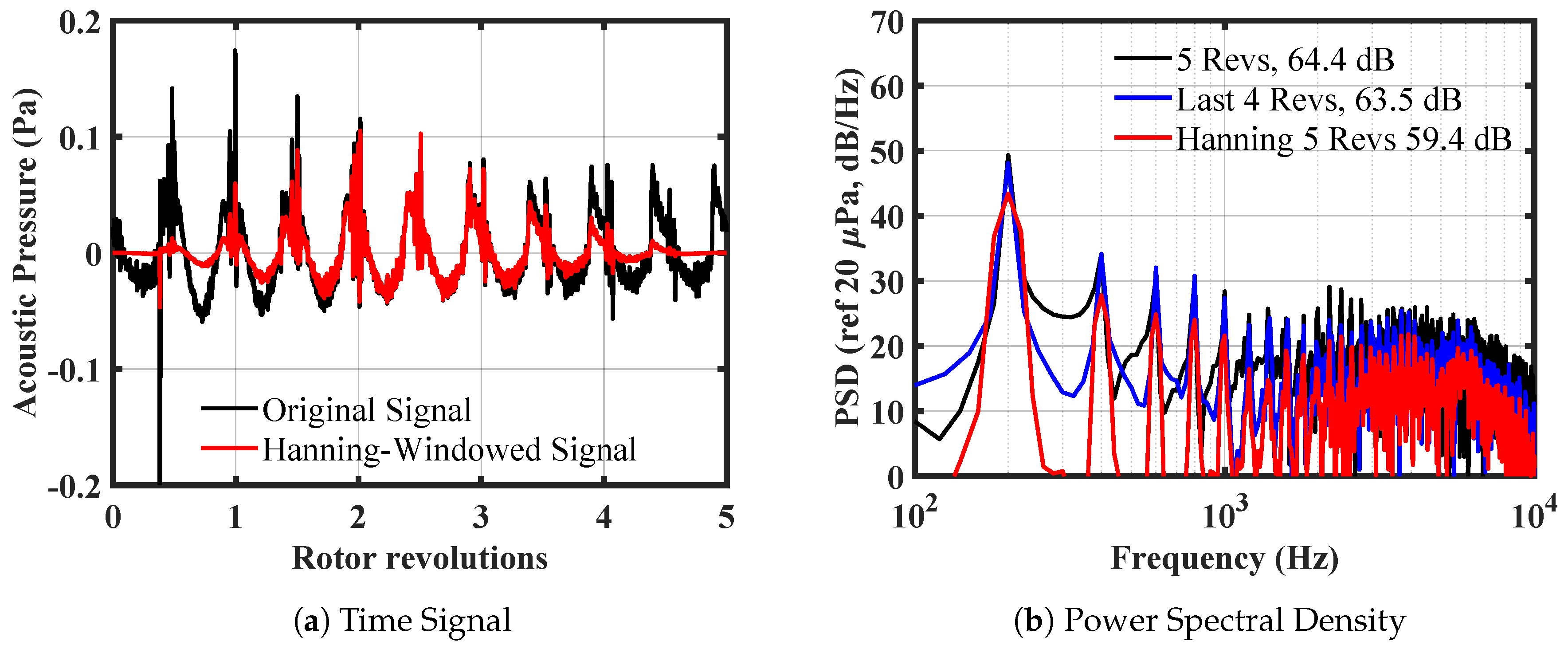
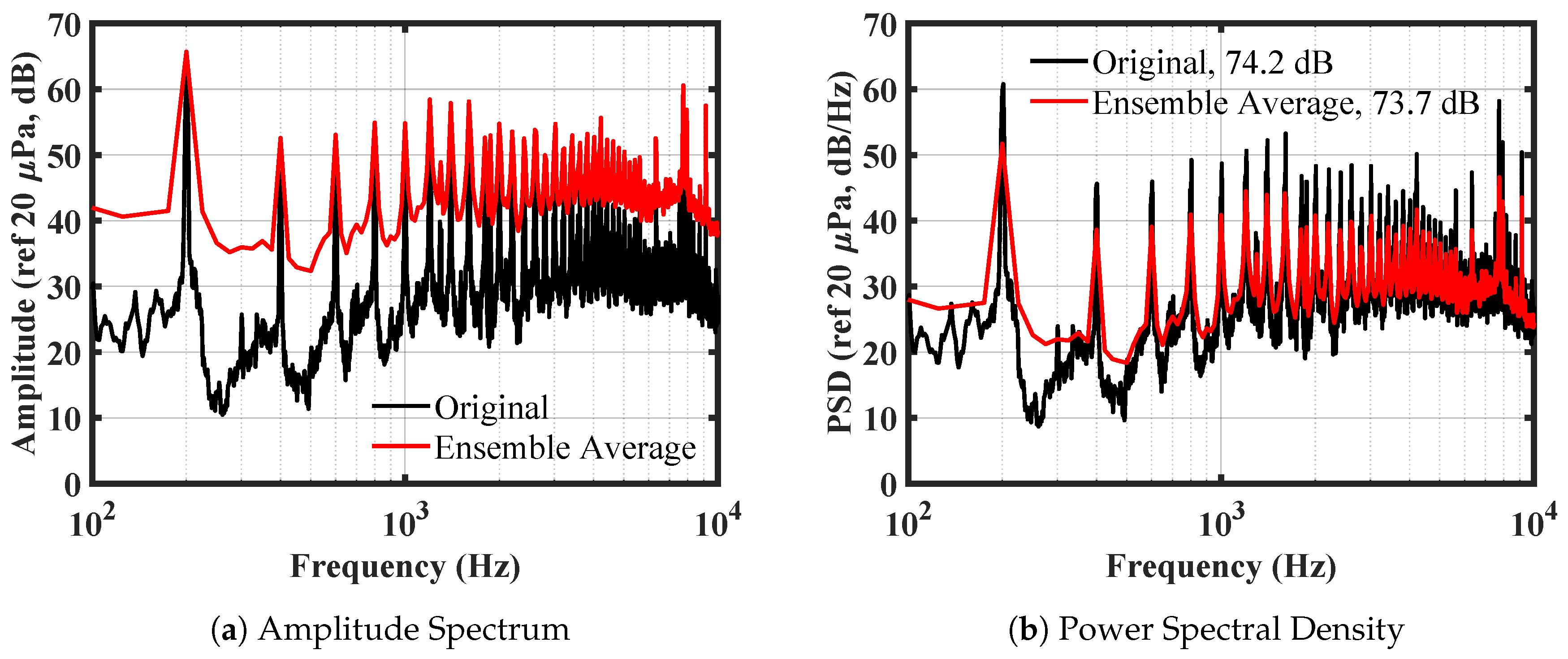
3.4. Processing of the Acoustic Signals

The acoustic signals measured in experiments and predicted computationally are compared. They are obtained using different sampling frequencies and sample lengths. There are many techniques used to prepare such data for comparison, and the methods used in this paper are described here. The processing of the computational data is discussed first. In PSU-WOPWOP, surface pressures are integrated to obtain the field pressure at the appropriate retarded time. Thus, the field pressure experiences a start-up effect in which there are no disturbances that have propagated to the point at the initial time, and as time progresses, disturbances from different surface locations begin to arrive. This start up manifests as a large pressure spike near the beginning of the audible time history. When the field pressure can be assumed to be periodic, the solver can assume that the end of the period can be wrapped into the beginning of the period filling in the disturbance information at the early times. Often, this leads to a regular field pressure signal. A drawback of the periodic assumption, though, is that only one period of computational data is used, which limits the frequency resolution of the associated spectrum.
To ensure better frequency resolution, five rotor revolutions were used for the acoustic integration in this paper. A periodic assumption was still made to try to avoid the effects of the initial acoustic spike. However, a spike still appeared in the first revolution as seen in Figure 4, which depicts the acoustic pressure signal at an above-plane observer of a dual rotor simulation, using Helios/PSU-WOPWOP. This most likely indicates that the simulation had not reached a perfectly periodic state when the acoustic integrals were started.
Researchers often employ a Hanning window when computing the spectrum of the acoustic signal [7,8,25]. It serves to dampen transient issues that can arise at the beginning and end of the pressure signal. A Hanning window is best used on longer signals than we have at our disposal in this work. Figure 4 shows the Hanning window applied to the five cycles of data we have at a given field point. The alteration to the signal at the beginning and end of the sampling can be seen in the left plot. The FFT of the original signal and the signal with the Hanning window applied is presented in the right plot. The Hanning window alters the tones and the broadband. Another approach to avoid the spike is to simply ignore the first revolution of the field pressure data. When an FFT is taken over the last four revolutions (and then adjusted for the differing frequency resolution via the power spectral density (PSD)), the nature of the signal is not as affected as when the Hanning window is applied as shown in Figure 4b. The overall sound pressure level was computed over the frequency band of 50 Hz to 10 kHz and included in the legend for each signal. The Hanning window dampens the energy of both the tones and the broadband. This results in a drop in the overall sound pressure level, compared to the other cases, and is not a good representation of the total noise. Therefore, the processing in this paper computes the acoustic pressure at the field point for five revolutions but will use only the last four revolutions to obtain the spectrum.
Next, the experimental measurements were prepared for comparison with simulations. The large sampling time of the experiments, 5 s, corresponds to 500 rotor revolutions. This leads to a frequency resolution much finer than that of the 4 or 5 rotor revolutions available from Helios/PSU-WOPWOP. The broadband amplitude spectra cannot be directly compared due to the differing frequency resolution. The PSD corrects for this difference by normalizing the spectral energy by the resolution, but should only be applied to the broadband, as the tones are unaffected by these issues, due to their periodicity. Therefore, ensemble averaging is typically employed to equalize the frequency resolution of the experiments with the simulations. Thus, an ensemble of 4 rotor revolutions was employed with no overlap, and the mean frequency spectrum of all ensembles is considered the ensemble average. The amplitude spectrum of the ensemble average, with a frequency resolution of 25 Hz, is compared to that of the original signal produced in De Paola’s thesis at a frequency resolution of 1.5 Hz in Figure 5a. As previously discussed, the amplitude spectrum of the ensemble average is shown to be higher than the original signal, due to the coarser frequency resolution. Thus, the PSD is calculated to account for this effect and shown in Figure 5b. The broadband matches well and the tones are slightly reduced, due to the spread of energy into neighboring frequency bins. However, the OASPL, shown in the legend, is similar because the energy of the entire spectrum is conserved. The small difference of 0.5 dB is caused by the numerical effects of averaging and is considered to be negligible enough for comparison with the simulations. The PSD of this ensemble averaged experimental data is, therefore, suitable for comparison with the PSD of the Helios/PSU-WOPWOP results.
Finally, the Helios/PSU-WOPWOP impermeable surface–based calculations are not able to capture the trailing edge noise. Therefore, the Helios/PSU-WOPWOP impermeable results are combined with the broadband noise predicted by UCD-Quietfly. To demonstrate this effect, the noise of each separate component as well as the total noise is plotted in Figure 6. The largest increase from the Helios/PSU-WOPWOP results occurs in the high frequency broadband, where the noise was relatively low. The combination of Helios/PSU-WOPWOP impermeable surface–based pressure and UCD-Quietfly broadband pressure is used throughout the paper.

4. Results

4.1. Performance Measurements and Predictions

The aerodynamic performance results of the isolated rotor and dual rotor configurations are discussed in this section.

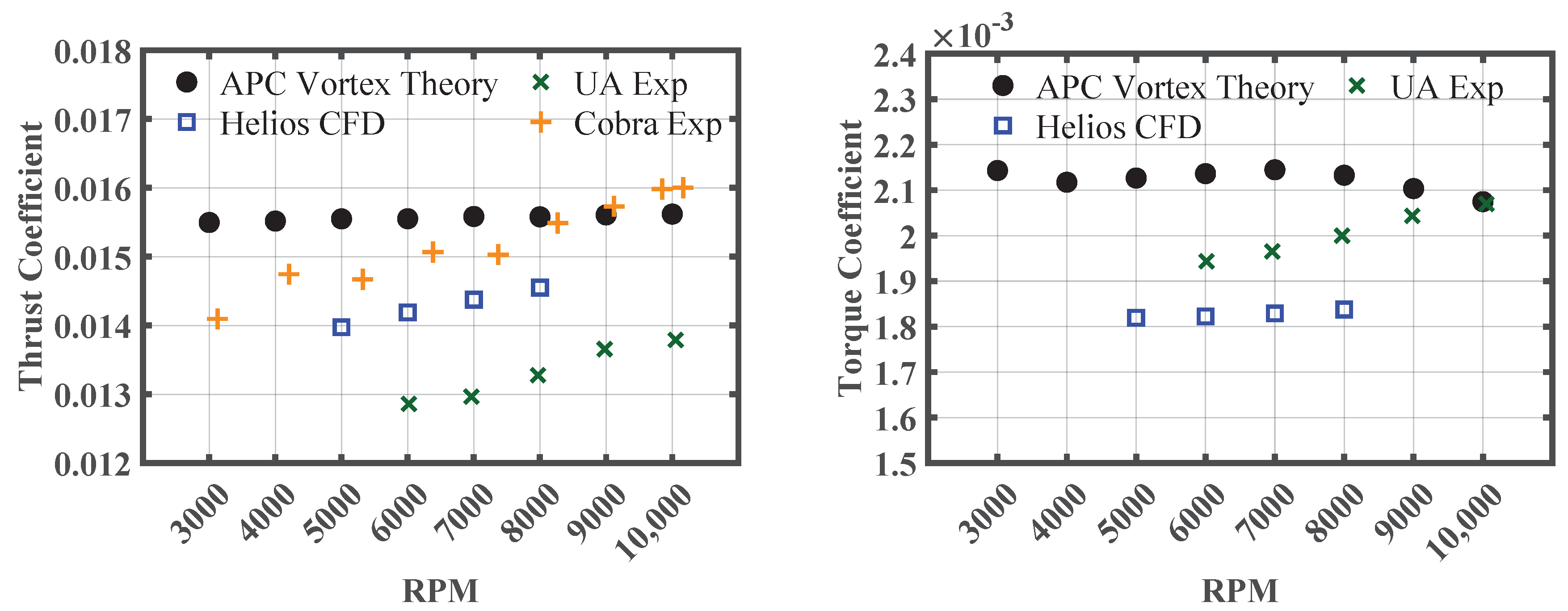
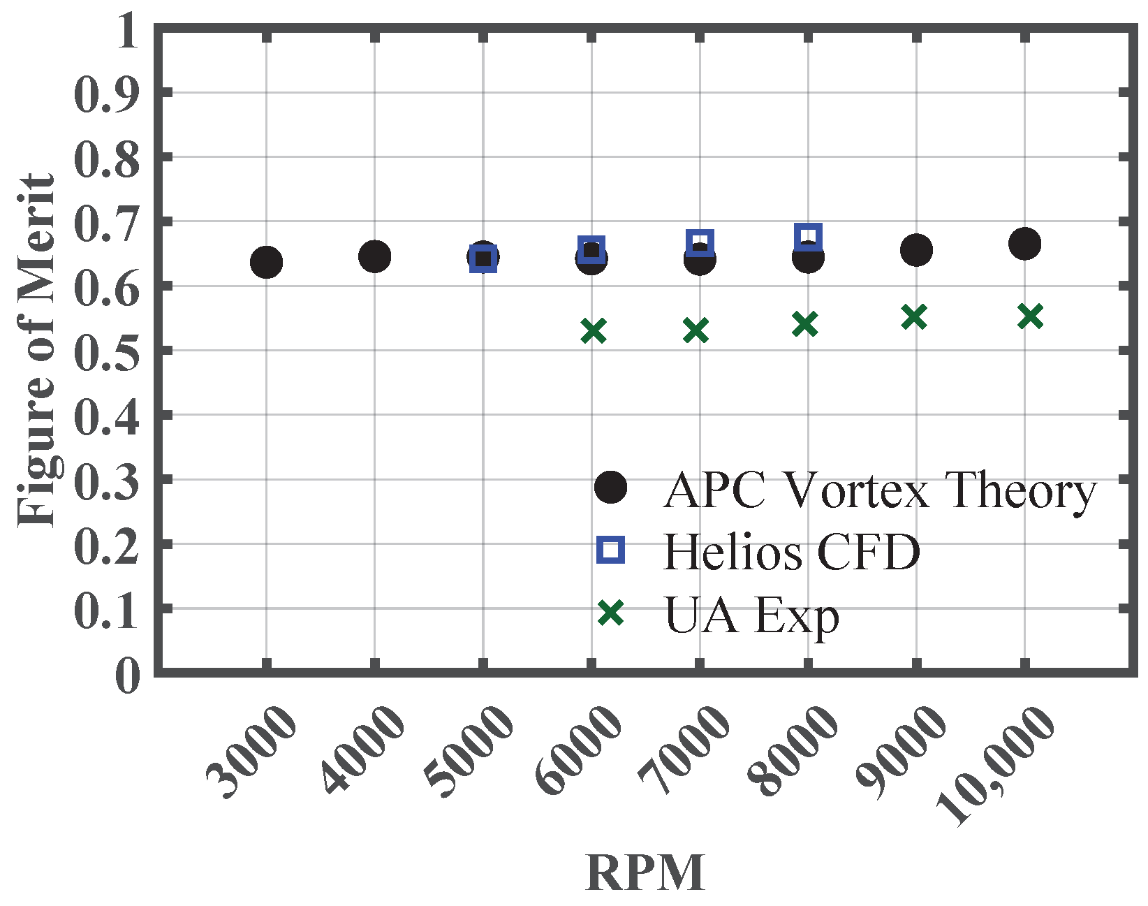
4.1.1. Isolated Rotor
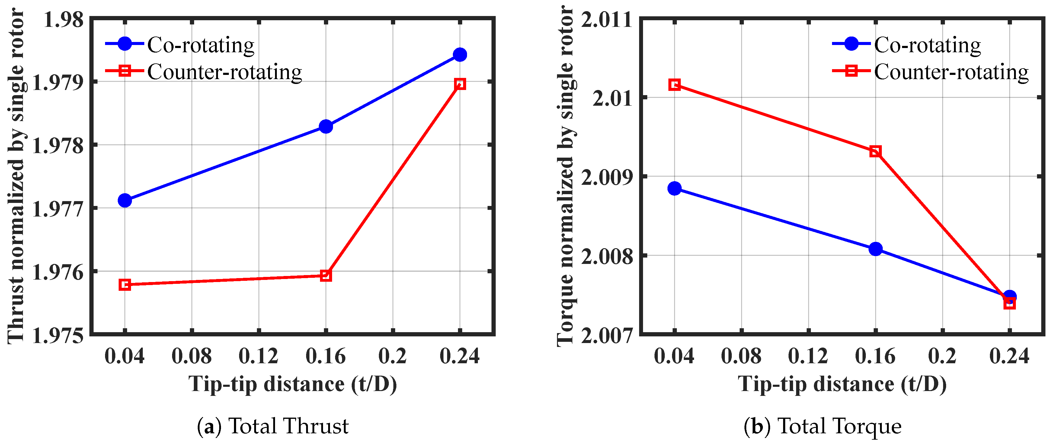
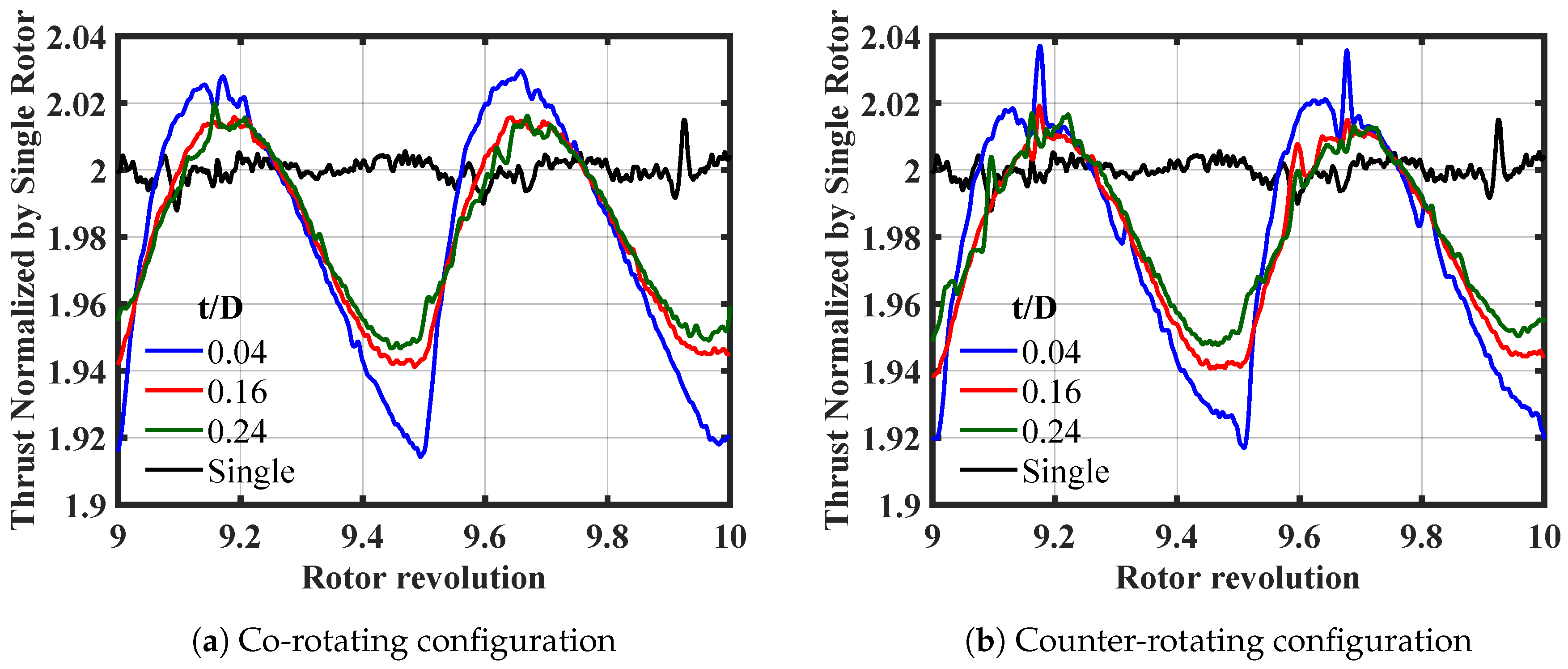
Rotor performance values are calculated as the mean over the tenth, and final, rotor revolution. The isolated rotor performance results of this paper are compared with other available data for the APC 8x4.5-MR rotor in the literature and in industry. Experiments conducted by Arterburn et al. at the University of Alabama, referred to as UA in this paper, measured thrust and torque using the RC Benchmark Series 1580 Dynamometer [64]. The rotor was also tested, using the Cobra CM-2206/30 Motor. The thrust data are available on the Innov8tive Designs website [65]. This work will be referred to as Cobra data. Only thrust was measured. Finally, we also include the manufacturer-reported performance data available on the APC that are computed using vortex theory [66].
The thrust coefficient C T = T / ( ρ π R 4 Ω 2 ) , where T is the thrust, ρ is the air density, R is the rotor radius, and Ω is the rotor rotation rate and the torque coefficient C Q = Q / ( ρ π R 5 Ω 2 ) , where Q is the torque are plotted in Figure 7. The CFD results are in reasonable agreement with the experimental data. However, the scatter in the experimental data further highlights the difficulty of characterizing a rotor’s performance. While the UA thrust values were obtained using an industry standard benchmark measurement device, they seem quite low. This is also confirmed by initial thrust measurements of the same rotor at BU performed using a JR3 Multi-Axis Force/Torque Sensor, which are closer to the Cobra and Helios results. The low value could be due to a calibration issue in the experiment. Even given all of these challenges faced when attempting validation, one can draw some general conclusions. Both the CFD and the experiments show an overall increasing trend with RPM for both thrust and torque coefficient values, which is not present in the APC inviscid calculation. This points to a Reynolds number effect that can only be captured with CFD.
The rotor figure of merit is a measure of hovering efficiency defined as η = C T 3 / 2 / ( 2 C Q ) [67]. A comparison of experimental and computed values for the APC rotor is plotted in Figure 8. The Helios results compare well with APC, even though the APC vortex theory predicted higher thrust and torque coefficients than Helios. When compared to UA, the computed FOM is higher, due to the low thrust value recorded by UA. Previous CFD results using fully-turbulent turbulence models have shown low figure of merit predictions, due to failure to capture boundary layer transition and separation [23,39]. The current results would, therefore, indicate that the flow is largely turbulent over this rotor, which allows the simulation to give a good prediction of FOM.

4.1.2. Dual Rotor

To explore the impact of rotor interactions, a pair of co-rotating counter-clockwise rotors and a pair of counter-rotating rotors were simulated using Helios. The 6000 RPM case was chosen, and the rotors were placed at tip-to-tip separation distances of t = 0.04 D , t = 0.16 D , and t = 0.24 D , where t is the tip-to-tip separation distance and D is the rotor diameter. The mean thrust of the entire system and the sum of the torques of the two rotors were normalized by the single rotor values and plotted in Figure 9. As expected, the interactions of the dual rotors reduce the performance of the individual rotors and lead to lower thrust and higher torque than the ideal value of 2. The expected trend is captured in which both performance parameters approach the ideal value of 2 with increasing distance. Another interesting result is the sensitivity of the performance parameters to the interactions. The thrust reduced by more than 1% for each rotor in the dual rotor system, compared to the isolated rotor, but the torque is only reduced by less than 0.5%, on average. Although these differences are negligible and may not be noticeable on a real propeller subject to external factors, the computations indicate that the interactions and induced flow are stronger perpendicular to the rotor plane.
The counter-rotating configuration demonstrates lower thrust and greater torque overall, due to a higher number of interactions. The trends of the counter-rotating configuration are not as well behaved as those of the co-rotating case, due to the unsteadiness in the thrust signal caused by the interactions. To show this, the thrust signal over the final rotor revolution is plotted in Figure 10 for both configurations. The thrust signal of the single rotor was doubled and plotted in black for comparison. All values were again normalized by the mean thrust over the final rotor revolution of the single rotor. The amplitude of the thrust oscillation clearly increases with the presence of a second rotor. The results show that increasing the rotor proximity increases the amplitude of the thrust oscillation, which will increase the noise. In addition, the unsteady behavior of the counter-rotating configuration is highlighted by a strong impulsive increase in thrust directly after the blade crossing, seen in Figure 10b. This impulse is not seen in the torque signal, emphasizing the larger interactional effects perpendicular to the rotor plane.
The flowfields of the dual rotors at the closest separation distance of t = 0.04 D were extracted from the simulation at the last time step to provide insight into the flow physics. A planar slice of vorticity magnitude across the rotors’ centerline can be seen in Figure 11. Iso-surfaces of q-criterion = 0.001 colored by the vorticity magnitude are shown in Figure 12. Both the co-rotating configuration and counter-rotating configuration are pictured. The same omega-shaped, horseshoe vortex predicted and measured in Refs. [27,31,33,35] can be seen in the counter-rotating configuration between the two rotors in Figure 12b. This vortex is generated by the interaction between the tip vortices of the two rotors; here, it is shown to be stronger for the counter-rotating case, indicated by the high vorticity band noticeable in Figure 11b, which is not visible in Figure 11a.
The co-rotating configuration displays more significant mixing in the wake below the gap region but does not generate the omega-shaped vortex and has little associated interaction effect appearing in its thrust signal. This mixing is not present for the counter-rotating rotors, due to induced upwash in the gap region. To demonstrate this effect, a slice of the downward vertical velocity is shown in Figure 13. The image of the downwash velocity is qualitatively similar to the PIV measurements of Zhou et al. [27]. These phenomena are not significant at the other distances simulated, which are sufficiently far enough to minimize interactions. A more careful study of the effect of this omega vortex at higher resolution intervals of the separation distance could be conducted in the future.

4.2. Aeroacoustics Measurements and Predictions

The aeroacoustics measurements and predictions of the isolated and dual rotor configurations are discussed in this section.

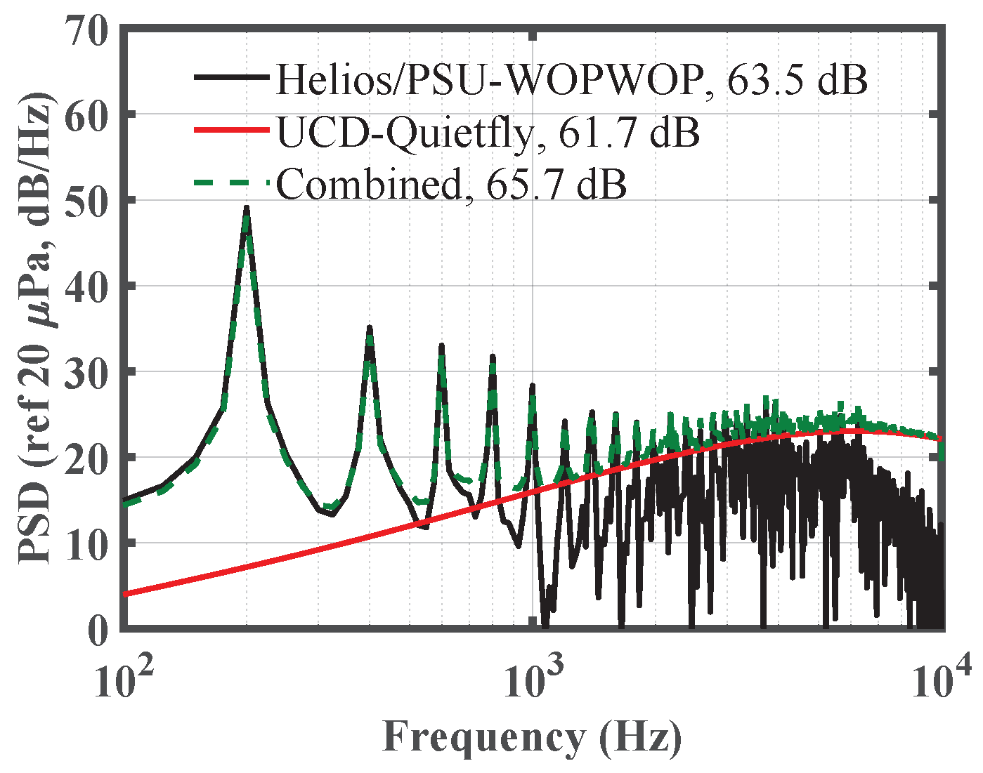
4.2.1. Isolated Rotor Noise Sources

The sound pressure level measured at Mic 3 of the azimuthal array, representing an in-plane observer, and Mic 3 of the linear array, representing an above-plane observer, are plotted in Figure 14 against predictions using combined Helios/PSU-WOPWOP with UCD-Quietfly. The in-plane mic shows an overprediction at the BPF and reasonable agreement at the second BPF harmonic. Although the azimuthal directivity of the isolated rotor should be uniform due to the symmetric loading, there were experimental installation effects which impacted the results. These effects showed a greater impact on tonal noise, and can explain the discrepancy in results when comparing a single mic location. The details of this discovery are explained further in Appendix A. Although the relative magnitude of the tones varied slightly, the higher harmonic tones present in the experiment were still noticeable around the entire azimuth. These tones are not present in the predictions, as there are no higher harmonic amplitudes that stand out from the broadband signal. On the other hand, the computations at the above-plane mic demonstrate some weak harmonics into the 5 kHz range. The thickness and loading acoustic pressure signals of the isolated rotor at the two mic locations are plotted in Figure 15. We see that the thickness contribution is fairly smooth and a low source of noise mainly at the BPF at both mics. The loading noise contribution is shown to dominate and contains slightly higher harmonic content, which is more prevalent at the out-of-plane mic than the in-plane mic. As an aside, BEMT predictions of the thrust are uniform around the azimuth, due to the steady leading of the blade and as such, would predict only noise at the BPF. This was demonstrated previously [24].
In previous papers that discuss the presence of higher harmonics, they are attributed to recirculation [4], random motor fluctuations [22], or self-generated turbulent inflow. Since the effects of recirculation and motor fluctuations are not modeled here, it must be the self-generated turbulent inflow that is responsible for the higher harmonics in the CFD simulations. However, the amplitude of the harmonics predicted by the computational methodology is low compared to the experimental measurements, which is most likely because the recirculation effect is not modeled. The low higher harmonic amplitudes match the findings of LBM predictions by Casalino et al. [25].
Turbulent inflow will also contribute to the broadband noise as will blade–wake interactions. These mechanisms are considered leading edge interactions as opposed to the trailing edge mechanisms modeled by UCD-Quietfly and have been shown to mainly affect the lower frequency [21]. The underprediction of the broadband by the present methodology in the frequency range under 1 kHz may indicate that the leading edge interaction is not fully resolved by the computation. The trailing edge contribution to the broadband is fairly well predicted, except that it has a more uniform directivity with a similar broadband hump occurring at high frequencies for both observers. The overprediction of the in-plane high frequency broadband by UCD-Quietfly as compared to the present experimental data is not understood at this time.

4.2.2. Choice of Integration Surface

A permeable surface calculation was conducted to quantify the influence of quadrupole sources. Mankbadi et al. posited that this source was significant for the broadband noise component, due to wake interactions that would not be captured with a surface integration [7]. It is also hypothesized here that the permeable surface should capture the pressure scattering predicted by the trailing edge model in UCD-Quietfly. Therefore, the Helios/PSU-WOPWOP + UCD-Quietfly results for the impermeable surface are compared with the standalone Helios/PSU-WOPWOP permeable surface calculations. The results for an in-plane and above-plane observer listening to the isolated rotor in hover at 6000 RPM are plotted in Figure 16. The experimental measurements are included for reference.
Focusing first on the in-plane results, there is a noticeable overall increase in noise at the first BPF. However, the broadband shape and amplitude are predicted with reasonable agreement. The permeable surface prediction reflects the relative flat broadband of the experiment, compared to the UCD-Quietfly predictions. The permeable surface also demonstrates excellent agreement for the above-plane observer. Previously, Mankbadi et al. showed much better agreement with the predicted BPF, using the two methods [7]. The large difference at the BPF shown here suggests the influence of hydrodynamic waves, which may be caused when the permeable surface is too close to the body. In addition, the comparison with experiments makes it even more difficult to validate either method because the impermeable integration matches in-plane but the permeable integration matches above-plane. It is unlikely that the computed noise at the BPF could be greater than that of the experiments because of the lack of recirculation in the simulations. Therefore, the current study will continue using the impermeable surface integration method for predictions. Future work will focus on identifying the effect of placement and topology of the permeable surface.

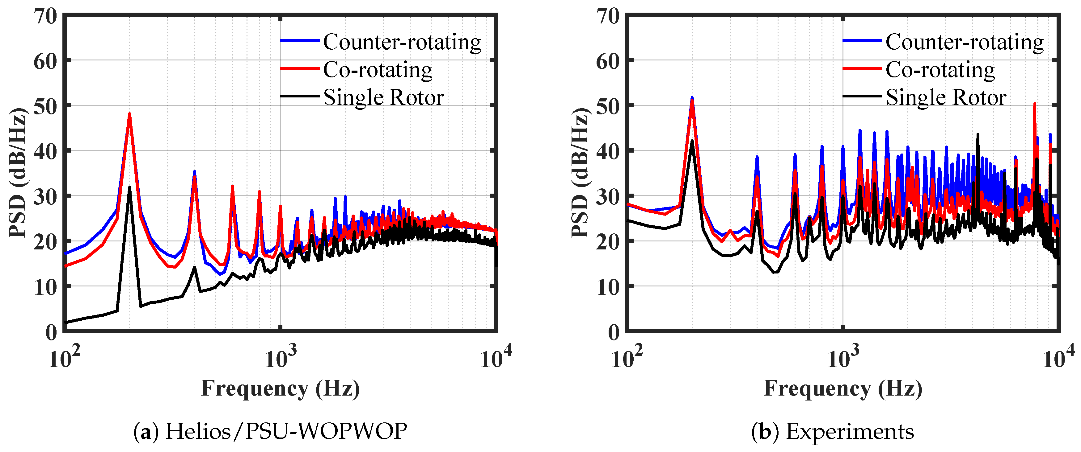
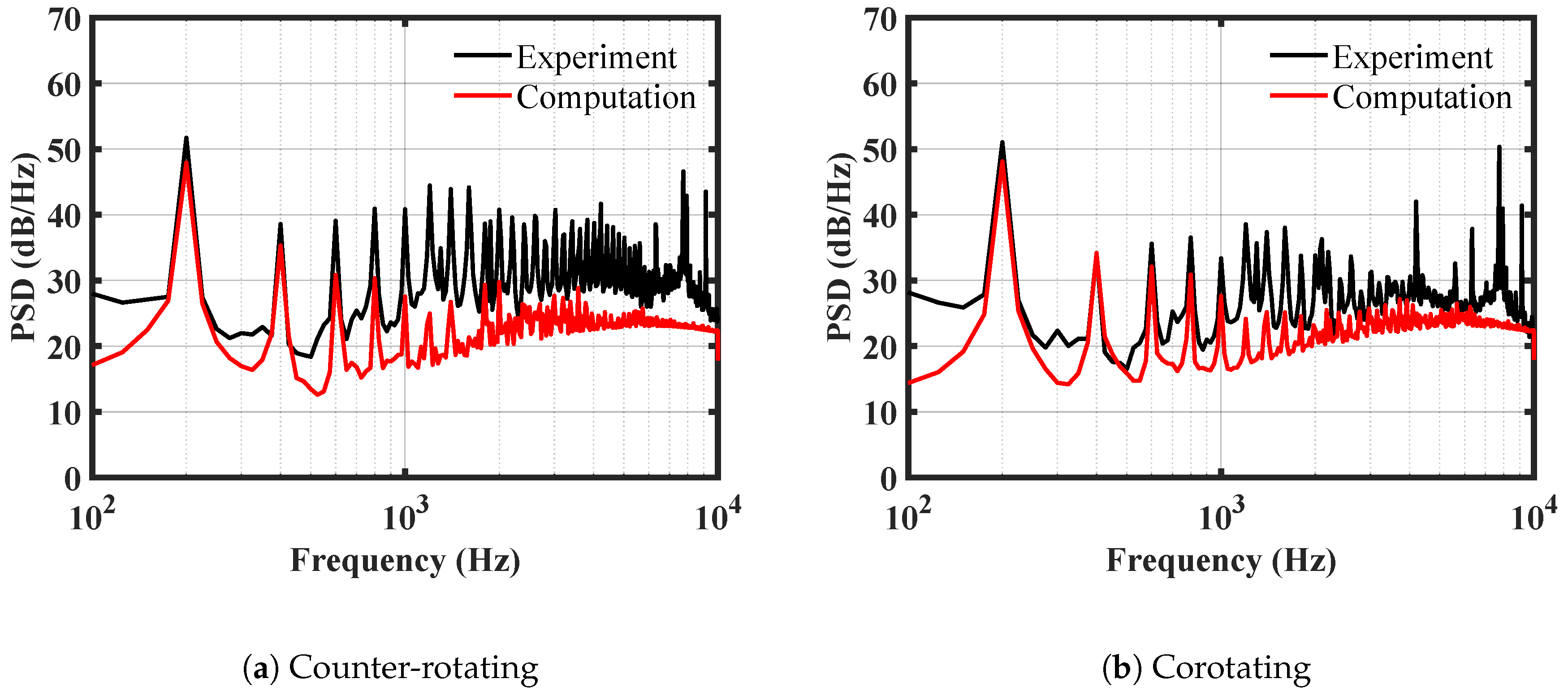
4.2.3. Dual Rotor Interactions

The interactional aerodynamics of the dual rotors predicted by Helios suggests an increase in noise from the single rotor case. The computed and measured sound at mic 3 of the linear array for the dual rotor configuration is plotted in Figure 17. The Helios/PSU-WOPWOP results show a significant increase in noise from the isolated rotor case, with greater than 15 dB increase at the BPF. This is greater than the effect of a pressure doubling, which means the computational methodology is able to capture the effect of the interaction. The experiment is also able to capture this effect, although it is less severe.
An even greater interactional effect lies in the higher harmonics. Although the single rotor simulations do show some weak harmonics, the dual rotor simulations are rich with strong BPF tones into the 2 kHz range. Zawodny et al. were able to identify increases in higher harmonic noise with the installation of different obstructions in the wake that represented a typical airframe [3]. These results indicate that the presence of an additional rotor is able to induce periodic unsteady loading, due to the impact of the blade-crossover events. The experiments show stronger higher harmonics for the dual rotor case as compared to the single rotor and they are much higher than predicted. This is, again, attributed to the effect of recirculation in the experiment, which is not modeled computationally.
It is interesting to note that the high frequency broadband of the Helios/PSU-WOPWOP results shows a negligible change between the isolated rotor and dual rotor configurations. This is attributed to the fact that the influence of the vortices of the adjacent rotor is due largely to leading edge interactions, whereas the high frequency broadband is sourced at the trailing edge. Nardari et al.’s experiments of a confined rotor also found that flow recirculation did not increase the trailing edge noise in the high frequency by much, and localized the increase in low-frequency noise at the leading edge [21]. This result is reflected in the present study, where the simulated low frequency broadband of the dual rotor is much greater than that of the single rotor.
Direct comparison between the computed results and experimental data at Mic 3 of the linear array for the co and counter rotating rotors at t = 0.04 D is provided in Figure 18 There is negligible difference in the broadband between the two configurations for the computations. The Helios/PSU-WOPWOP method resolves the acoustics in the low frequency, due to the leading edge interactions, while the UCD-Quietfly models the high frequency trailing edge noise. Therefore, the shape of the broadband shows excellent agreement with the experiments, although the amplitude is slightly low. It is possible that neither Helios/PSU-WOPWOP nor UCD-Quietfly is able to capture the effect of the blade wake or blade vortex interactions on the trailing edge noise, which would be greater for the dual-rotor case.

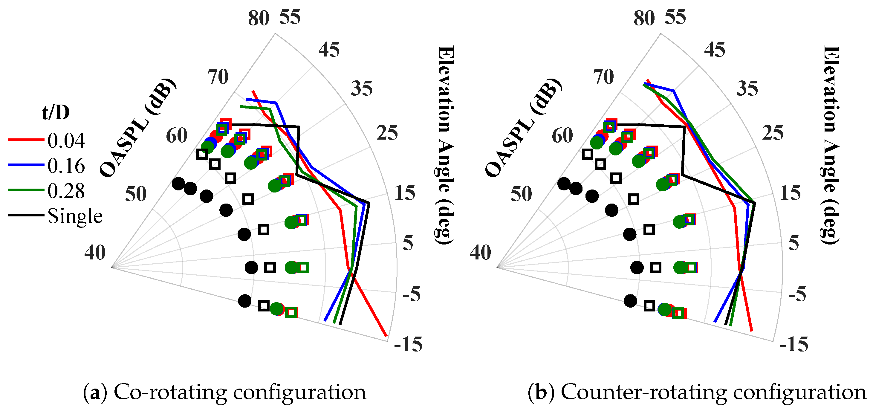
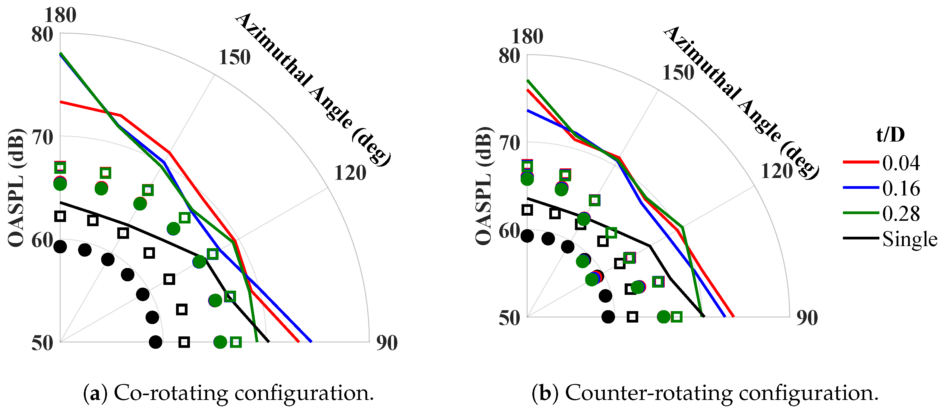
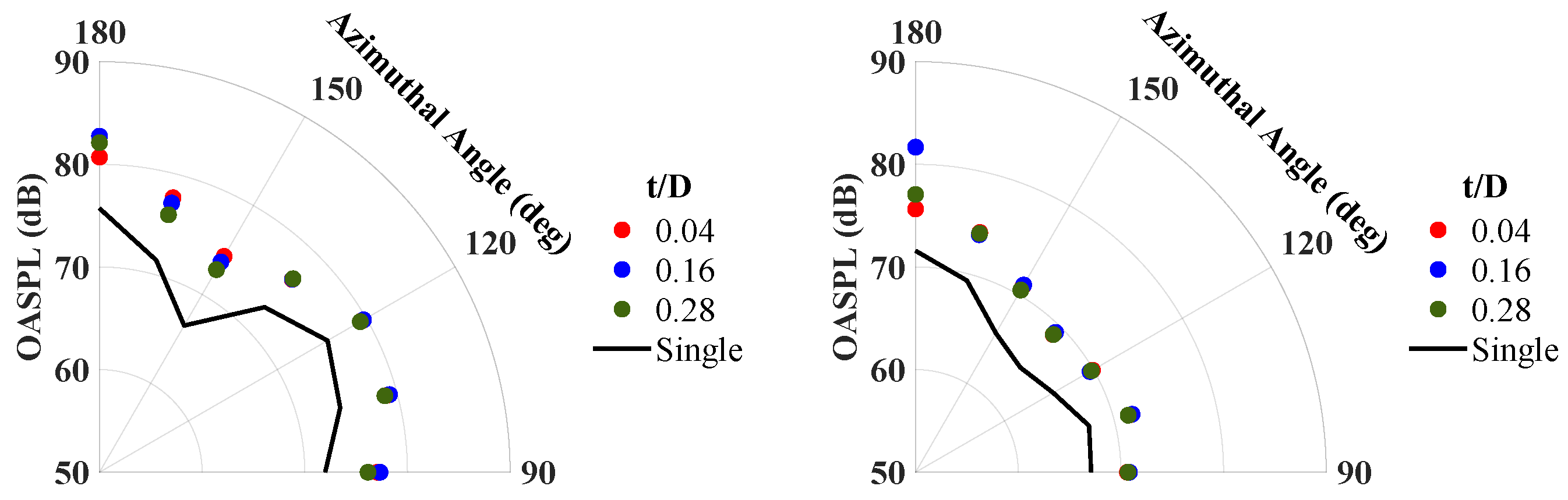
4.2.4. Overall Sound Pressure Level and Directivity

To combine the acoustic results across the multitude of cases run, the directivity of the total sound is addressed in this section. The overall sound pressure level (OASPL) is used as a metric for the total sound across both tonal and broadband components and is defined here as the integral of the PSD in the frequency band of 50 Hz to 10 kHz.
The polar directivity of both dual rotor configurations is shown in Figure 19. The experimental values are shown as lines, the combined Helios/PSU-WOPWOP and UCD-Quietfly results are shown as squares, and the standalone Helios/PSU-WOPWOP results are shown as circles. It is obvious from the results in previous sections, including the acoustic spectra, that the OASPL of the experiments would be much greater than that of the single rotor computation due to the impact of other effects, including recirculation, unsteady motor vibration, motor noise, and any potential structural dynamics. These factors, in addition to installation effects, may explain the lack of trend across the different tip separation distances of the dual rotor measurements. The factors make it particularly difficult to see the expected trend between single and dual rotor experimental results. Validation of the computational predictions with the experimental data is not possible. If one has some faith that the computations provide good predictions for rotors in a free field environment void of motor noise, etc., then a few conclusions follow. (1) Rotor–rotor interactions lead to higher harmonics that are on the order of, or greater than, higher harmonics caused by recirculation. (2) The polar directivity between −15 deg and 15 deg is symmetric for the single rotor, but greater above-plane for the dual rotor. In general, the largest OASPL is seen near the rotor plane. (3) Both configurations show similar directivity. (4) The contribution of the trailing edge broadband noise to the OASPL is proportionally greater for the single rotor than the dual rotor, due to the relative amplitude of the BPF. (5) The decreasing tip distance between the dual rotors barely affects the noise from −15 degrees to 25 degrees and increases the noise by a few dB at a higher elevation. The influence of rotor proximity has a greater impact on above-plane noise than thrust, highlighting the fact that the noise is more susceptible to interactions than interaction.
Next, the azimuthal directivity of the noise is plotted in Figure 20. The authors again refer the reader to Appendix A for insight into the asymmetry of the experimental OASPL. The predicted acoustic magnitude is lower than experiment as expected, given the aforementioned environmental effects. The co-rotating configuration demonstrates a uniform directivity around the azimuth, while the counter-rotating configuration shows a reduction in OASPL between 120 deg and 150 deg, even beyond the magnitudes of the single rotor. The reduction is due to destructive interference of the tones of in-phase counter-rotating rotors. These results are in agreement with those of Pascioni et al. and Schiller et al., who compared computations and experiments of counter-rotating and co-rotating side-by-side rotors and found interesting directivity patterns in-plane depending on the phasing [68,69]. They concluded that exact rotor phasing and less than 0.5% variation in the RPM were required to produce the destructive interference. It is not surprising then that the experiments, which are not phase locked, do not show as dramatic of a reduction in the OASPL from 120 deg to 150 deg for the counter-rotating case.

5. Conclusions

In this paper, the aeroacoustic interactions of small rotors in hover were evaluated experimentally and computationally. The APC 8x4.5MR rotor was tested in both single and dual rotor hover configurations to quantify the effect of self-induced interactions as well as rotor–rotor interactions. Experimental performance values for the single rotor were taken from reports available online. Experimental acoustic values for single and dual rotors were obtained at University Roma Tre in an anechoic chamber, using a linear array of microphones oriented vertically to obtain the polar directivity and horizontally to obtain the azimuthal directivity. Computational predictions were obtained, using the CREATE-AV Helios suite coupled to PSU-WOWOP and UCD-Quietfly. The CFD employed DES, a hybrid URANS/LES method, and the PSU-WOPWOP was used to perform an impermeable surface Ffowcs-William and Hawkings calculation. UCD-Quietfly accounted for trailing edge broadband noise.
The predicted performance values and trends of the isolated rotor in hover were consistent with previously reported results. Differences between reported results are attributed here to manufacturing differences between the blades and possible experimental calibration errors. The predicted acoustic spectrum demonstrated reasonable first and second BPF for the in-plane mic when compared to the experiment, but did not predict the higher harmonics. All BPF harmonics were under-predicted for the above-plane observers. Due to the dominance of the loading noise effects above the plane, it was posited that the computations were not capturing the effects of recirculation. The UCD-Quietfly broadband modeling framework showed good prediction of the broadband shape and amplitude, although the in-plane results need further inspection.
No dual rotor performance values were available for comparison. Examination of the computed dual rotor performance trends showed decreasing mean thrust and increasing torque with increasing proximity. Increasing proximity also created large thrust fluctuations. For counter-rotating rotors, an impulsive type thrust response was seen and attributed to the interaction of the rotor and disturbances in the gap between the rotors. An omega-shaped vortex appeared in the gap that qualitatively matched computations and PIV measurements of prior works.
The dual rotor acoustic predictions showed higher harmonic noise, indicating that the effects of the interaction are more significant than those of the recirculation for dual rotors. The broadband shape of the combined Helios/PSU-WOPWOP and UCD-Quietfly results showed excellent agreement with the experiment, although the amplitude was low. The counter-rotating configuration was shown to have greater noise than the co-rotating configuration above-plane, reflecting the aerodynamic performance trend. The azimuthal directivity of the counter-rotating rotors demonstrated the effects of destructive interference due to rotor-phasing and was much stronger in the computation, where the phasing is perfect, than in the experiment, which did not control for the rotor phase.
This work highlights how challenging it is to obtain experimental data for the validation of small rotor acoustics computations. It also shows the challenge for computations for application to realistic vehicle settings in which the rotors are not perfectly phased or at the exact same RPM, the flow near the rotors are disturbed by the rest of the vehicle’s structure, and the flow field may not be quiescent. It was demonstrated that high-fidelity CFD modeling captures a Reynolds number performance effect that inviscid models do not capture. It was also shown that the high-fidelity CFD model can capture the impact of interactional effects on the creation of higher harmonics. The high-fidelity CFD together with an impermeable surface FWH, however, does not capture all of the noise sources; their effect was added via the use of UCD-Quietfly. The single rotor permeable surface FWH calculation presented in the paper suggests that more of the noise sources are captured using the permeable surface. However, an inconsistency in the BPF prediction with the permeable surface called into question the accuracy of this implementation. It is surmised that the issue is due to imperfect placement or topology of the surface, which requires further investigation. The Helios/PSU-WOPWOP simulation framework requires computational resources for the dual rotor cases on the order of 10 5 CPU hours. Such computations are not helpful for design, but will continue to help identify important contributors to the performance and acoustics of different multi-rotor configurations.

Author Contributions

Conceptualization, A.D.T., S.M.G.; methodology, A.D.T., S.M.G.; software, A.D.T.; validation, A.D.T., S.M.G.; formal analysis, A.D.T., S.M.G.; investigation, A.D.T., E.D.P., L.G.S., A.D.M., S.M.G.; resources, A.D.T., R.C., S.M.G.; data curation, A.D.T., E.D.P., L.G.S., A.D.M., S.M.G.; writing—original draft preparation, A.D.T., E.D.P., S.M.G.; writing—review and editing, A.D.T., E.D.P., S.M.G.; visualization, A.D.T.; supervision, A.D.M., R.C., R.T., S.M.G.; project administration, R.T., S.M.G.; funding acquisition, R.T., S.M.G. All authors have read and agreed to the published version of the manuscript.

Funding

The computational aspect of this research was partially funded by NSF Grant Number 1728277 and the Boston University Mechanical Engineering Department. The U.S. Army provided the computational resources, funding support, and software for the first author through the Department of Defense High Performance Computing Modernization Program.

Institutional Review Board Statement

Not applicable.

Informed Consent Statement

Not applicable.

Data Availability Statement

The data can be obtained upon request from the corresponding author.

Acknowledgments

APC, the manufacturer of the rotor used in this study, provided the CAD model of the rotor geometry. Roger Strawn and Andy Wissink provided the computing hours and administrated the internships of the first author. Mark Potsdam provided the software for the coupling between Helios and PSU-WOPWOP. Kenneth Brentner provided the PSU-WOPWOP software and aided in Helios/PSU-WOPWOP coupling. Sicheng Li and Seongkyu Lee provided the UCD-Quietfly code. W. Nathan Alexander, Damiano Casalino, and Nikolas Zawodny provided insight into the higher harmonic noise. The experimental test campaign was carried out in support of the EU funded CLEAN SKY 2 Joint Undertaking Project ERACLE (Grant Agreement No. 687015-8).

Conflicts of Interest

The authors declare no conflict of interest. The funders had no role in the design of the study; in the collection, analyses, or interpretation of data; in the writing of the manuscript, or in the decision to publish the results.

Abbreviations

The following abbreviations are used in this manuscript:
AMRAdaptive Mesh Refinement
BPFBlade Passage Frequency
BPMBrooks, Pope, and Marcolini
CAAComputational Aeroacoustics
CADComputer-Aided Design
CFDComputational Fluid Dynamics
DNSDirect Numerical Simulation
DoDDepartment of Defense
eVTOLElectric Vertical Take-off and Landing
FWHFfowcs-Williams Hawking
HPCMPHigh Performance Computing Modernization Program
NSNavier–Stokes
LBMLattice Boltzmann Methods
LESLarge Eddy Simulation
OASPLOverall Sound Pressure Level
RPMRevolutions per minute
PWLPower Watt Level
SPLSound Pressure Level
VPMVortex Particle Method
UAMUrban Air Mobility
UAVUnmanned Aerial Vehicles
URANSUnsteady Reynolds-Averaged Navier–Stokes

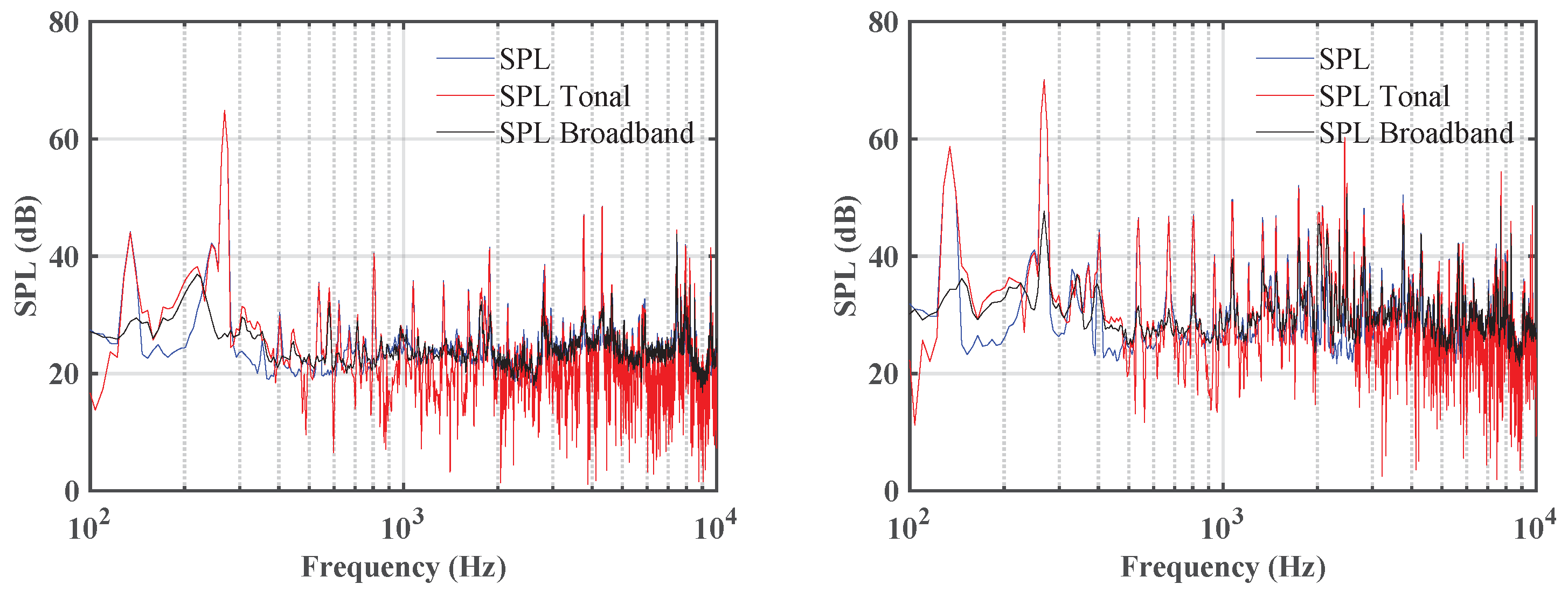
Appendix A. Tonal and Broadband Noise Separation

The analysis of the experimental data showed a dependence of the azimuthal directivity on the rotational speed of the rotors. In particular, both for the single and twin-rotor configuration, the OASPL curves exhibited a significant variation in curvature as RPM increases. However, especially in the single propeller case, by approximating the noise source as a monopole, one would have expected a uniform trend along the microphone array, which is not the case in the experimental results. To better clarify the reasons behind the nonuniform directivity, a signal decomposition method was used to separate the sound pressure spectrum into the two components of tonal and broadband contributions.
The method followed for the tonal and broadband noise separation is the one presented by Sree and Stephens [70], usually adopted to separate open rotor acoustic data, based on the removal of an average tonal waveform.
In particular, the technique involves the following steps. First, divide the raw acoustic data into uniform segments, take two consecutive ones, and perform a cross-correlation operation to realign and phase-adjust them. In this way, each segment is composed of a common tone component plus a realization of a stationary random part that can be isolated by canceling the tone portion of the signal, which is coherent between the segments. Doing this for the all raw signal length allows building a pseudo time-series of the broadband signal. However, appending the individual broadband segments will create discontinuity at each junction and, thus, introduce a small amount of white noise into the computed spectrum. This effect can be mitigated using a smoothing window, such as Hanning, with each segment. A long time-series of the broadband signal is reconstructed, having the total length equal to about one-half of that of the original raw data set. An FFT operation is now performed to obtain the broadband spectral values as a function of frequency, which can be subtracted to the averaged total spectrum to obtain the tonal contribution.
The major drawback of this method is that the broadband spectrum may contain irregular, tone-like spikes, due to unaccounted random phase shifts occurring in the data segment-pairs selected for the cross-correlation operation. In addition, the spectrum of the random component may be slightly amplified as a result of the averaging operation in the frequency domain together with the use of smoothing windows. Despite this, the procedure was found to be particularly suited for the case of dual-rotor systems having approximately equal rotational speed [70,71]; it allows one to obtain a reasonable approximation of the broadband level. For both configurations, Figure A1 presents an example of the spectra obtained with the separation procedure at the ninth microphone ( θ = 180°) of the azimuthal array. The figures refer to a rotational speed of 8000 rpm and to the minimum separation distance ( t = 0.04 D ) of the dual propeller system.
The OASPL can now be computed by integrating the separated spectra to retrieve the directivities of each contribution. For the co-rotating case, Figure A2 illustrates the OASPL at each microphone for the three relative distances analyzed, t = 0.04 D , t = 0.16 D , t = 0.24 D , and the comparison with the isolated rotor configuration at 8000 rpm.
The modification in the shape of the curves with increasing rpm is mainly attributed to the behavior of the tonal noise, dominated by the trend of the first BPF, which suggests the presence of considerable installation effects. Being at static thrust conditions, a higher rotational speed results in more air being sucked in by the rotor; asymmetries due to the experimental set up in the upstream lead to a visible variation in the directivity patterns.

References

  1. Rizzi, S.A.; Huff, D.L.; D. Douglas Boyd, J.; Bent, P.; Henderson, B.S.; Pascioni, K.A.; Sargent, D.C.; Josephson, D.L.; Marsan, M.; He, H.; et al. Urban Air Mobility Noise: Current Practice, Gaps, and Recommendations; Technical Report TP-2020-5007433; NASA: Hampton, VA, USA, 2020.
  2. Intaratep, N.; Alexander, W.N.; Devenport, W.J.; Grace, S.M.; Dropkin, A. Experimental Study of Quadcopter Acoustics and Performance at Static Thrust Conditions. In Proceedings of the 22nd AIAA/Council of European Aerospace Studies Aeroacoustics Conference, Lyon, France, 30 May–1 June 2016. [Google Scholar] [CrossRef] [Green Version]
  3. Zawodny, N.S.; Boyd, D.D. Investigation of Rotor-Airframe Interaction Noise Associated with Small-Scale Rotary-Wing Unmanned Aircraft Systems. In Proceedings of the American Helicopter Society 73rd Annual Forum, Fort Worth, TX, USA, 8–11 May 2017. [Google Scholar]
  4. Weitsman, D.; Stephenson, J.H.; Zawodny, N.S. Effects of flow recirculation on acoustic and dynamic measurements of rotary-wing systems operating in closed anechoic chambers. J. Acoust. Soc. Am. 2020, 148, 1325–1336. [Google Scholar] [CrossRef] [PubMed]
  5. Whelchel, J.; Alexander, W.N.; Intaratep, N. Propeller Noise in Confined Anechoic and Open Environments. In Proceedings of the AIAA Scitech 2020 Forum, Orlando, FL, USA, 6–10 January 2020. [Google Scholar] [CrossRef]
  6. De Paola, E. Aeroacoustic Experimental Characterization of Rotor-to-Rotor Interaction Effects. Ph.D. Thesis, Roma Tre University, Rome, Italy, 2020. [Google Scholar]
  7. Mankbadi, R.R.; Afari, S.O.; Golubev, V.V. High-Fidelity Simulations of Noise Generation in a Propeller-Driven Unmanned Aerial Vehicle. AIAA J. 2021, 59, 1020–1039. [Google Scholar] [CrossRef]
  8. Casalino, D.; Grande, E.; Romani, G.; Ragni, D.; Avallone, F. Towards the definition of a benchmark for low Reynolds number propeller aeroacoustics. In Proceedings of the 18th International Symposium on Transport Phenomena and Dynamics of Rotating Machinery, Online, 23–26 November 2020. [Google Scholar]
  9. Spalart, P. Strategies for turbulence modelling and simulations. Int. J. Heat Fluid Flow 2000, 21, 252–263. [Google Scholar] [CrossRef]
  10. Jia, Z.; Lee, S. Impulsive Loading Noise of Lift-Offset Coaxial Rotor in High-Speed Forward Flight. AIAA J. 2020, 58, 687–701. [Google Scholar] [CrossRef]
  11. Jain, R. Sensitivity Study of High-Fidelity Hover Predictions on the Sikorsky S-76 Rotor. J. Aircr. 2018, 55, 78–88. [Google Scholar] [CrossRef]
  12. Thai, A.D.; Grace, S.M.; Jain, R. The Effect of Turbulence Modeling Selection within HPCMP CREATE-AV Helios for Small Quadrotor Aerodynamics. J. Aircr. 2021. in review. [Google Scholar]
  13. Chen, S.; Doolen, G.D. Lattice Boltzmann Method for Fluid Flows. Annu. Rev. Fluid Mech. 1998, 30, 329–364. [Google Scholar] [CrossRef] [Green Version]
  14. Williams, J.E.F.; Hawkings, D.L. Sound generation by turbulence and surfaces in arbitrary motion. Philos. Trans. R. Soc. Ser. A 1969, 264, 321–342. [Google Scholar] [CrossRef]
  15. Spalart, P.; Belyaev, K.V.; Shur, M.L.; Strelets, M.K.; Travin, A.K. On the differences in noise predictions based on solid and permeable surface Ffowcs Williams-Hawkings integral solutions. Int. J. Aeroacoustics 2019, 18, 621–646. [Google Scholar] [CrossRef]
  16. Lopes, L.V.; D. Douglas Boyd, J.; Nark, D.M.; Wiedemann, K.E. Identification of Spurious Signals from Permeable Ffowcs Williams and Hawkings Surfaces. In Proceedings of the American Helicopter Society 73rd Annual Forum, Fort Worth, TX, USA, 8–11 May 2017. [Google Scholar]
  17. Brooks, T.F.; Pope, D.S.; Marcolini, M.A. Airfoil Self-Noise and Prediction; Technical Report RP-1218; NASA: Hampton, VA, USA, 1989.
  18. Pettingill, N.A.; Zawodny, N.S. Identification and Prediction of Broadband Noise for a Small Quadcopter. In Proceedings of the 75th VFS Forum, Philadelphia, PA, USA, 13–16 May 2019. [Google Scholar]
  19. Russell, C.; Sekula, M. Comprehensive Analysis Modeling of Small-Scale UAS Rotors. In Proceedings of the American Helicopter Society 73rd Annual Forum, Fort Worth, TX, USA, 8–11 May 2017. [Google Scholar]
  20. Zawodny, N.S.; Boyd, D.D., Jr.; Burley, C.L. Acoustic Characterization and Prediction of Representative, Small-Scale Rotary-Wing Unmanned Aircraft System Components. In Proceedings of the American Helicopter Society 72nd Annual Forum, West Palm Beach, FL, USA, 16–19 May 2016. [Google Scholar]
  21. Nardari, C.; Casalino, D.; Polidoro, F.; Coralic, V.; Brodie, J.; Lew, P.T. Numerical and Experimental Investigation of Flow Confinement Effects on UAV Rotor Noise. In Proceedings of the 25th AIAA/Council of European Aerospace Studies Aeroacoustics Conference, Delft, The Netherlands, 20–23 May 2019. [Google Scholar] [CrossRef]
  22. McKay, R.S.; Kingan, M.J. Multirotor Unmanned Aerial System Propeller Noise Caused by Unsteady Blade Motion. In Proceedings of the 25th AIAA/Council of European Aerospace Societies Aeroacoustics Conference, Delft, The Netherlands, 20–23 May 2019. [Google Scholar] [CrossRef]
  23. Thai, A.D.; Grace, S.M. Prediction of Small Quadrotor Blade Induced Noise. In Proceedings of the 25th AIAA/Council of European Aerospace Societies Aeroacoustics Conference, Delft, The Netherlands, 20–23 May 2019. [Google Scholar] [CrossRef]
  24. Alvarez, E.J.; Schenk, A.; Critchfield, T.; Ning, A. Rotor-on-Rotor Aeroacoustic Interactions of Multirotor in Hover. In Proceedings of the Vertical Flight Society 76th Annual Forum, Online, 5–8 October 2020. [Google Scholar]
  25. Casalino, D.; Grande, E.; Romani, G.; Ragni, D.; Avallone, F. Definition of a benchmark for low Reynolds number propeller aeroacoustics. Aerosp. Sci. Technol. 2021, 113, 106707. [Google Scholar] [CrossRef]
  26. Kocheemoolayil, J.G.; Stitch, G.D.; Barad, M.F.; Kiris, C. Propeller Noise predictions using the Lattice Boltzmann Method. In Proceedings of the 25th AIAA/Council of European Aerospace Societies Aeroacoustics Conference, Delft, The Netherlands, 20–23 May 2019. [Google Scholar] [CrossRef]
  27. Zhou, W.; Ning, Z.; Li, H.; Hu, H. An Experimental Investigation on Rotor-to-Rotor Interactions of Small UAV. In Proceedings of the 35th AIAA Applied Aerodynamics Conference, Denver, CO, USA, 5–9 June 2017. [Google Scholar] [CrossRef] [Green Version]
  28. Shukla, D.; Komerath, N. Multirotor Drone Aerodynamic Interaction Investigation. Drones 2018, 2, 43. [Google Scholar] [CrossRef] [Green Version]
  29. Lee, H.; Lee, D.J. Rotor interactional effects on aerodynamic and noise characteristics of a small multirotor unmanned aerial vehicle. Phys. Fluids 2020, 32, 047107. [Google Scholar] [CrossRef] [Green Version]
  30. Bernardini, G.; Centracchio, F.; Gennaretti, M.; Iemma, U.; Pasquali, C.; Poggi, C.; Rossetti, M.; Serafini, J. Numerical Characteristics of the Aeroacoustic Signature of Propeller Arrays for Distributed Electric Propulsion. Appl. Sci. 2020, 10, 2643. [Google Scholar] [CrossRef] [Green Version]
  31. Afari, S.; Mankbadi, R.R. Simulations of Noise Generated by Rotor-Rotor Interactions at Static Conditions. In Proceedings of the AIAA Scitech 2021 Forum, Nashville, TN, USA, 11–15 January 2021. [Google Scholar] [CrossRef]
  32. Diaz, P.V.; Johnson, W.; Ahmad, J.; Yoon, S. Computational Study of the Side-by-Side Urban Air Taxi Concept. In Proceedings of the Vertical Flight Society 75th Annual Forum and Technology Display, Philadelphia, PA, USA, 13–16 May 2019. [Google Scholar]
  33. Sagaga, J.; Lee, S. CFD Hover Predictions for the Side-by-Side Urban Air Taxi Concept Rotor. In Proceedings of the AIAA Aviation 2020 Forum, Virtual, 15–19 June 2020. [Google Scholar] [CrossRef]
  34. Jia, Z.; Lee, S. Acoustic Analysis of Urban Air Mobility Quadrotor Aircraft. In Proceedings of the Vertical Flight Society Aeromechanics for Advanced Vertical Flight Technical Meeting, San Jose, CA, USA, 21–23 January 2020. [Google Scholar]
  35. Sagaga, J.; Lee, S. Acoustic Predictions for the Side-by-Side Air Taxi Rotor in Hover. In Proceedings of the 77th VFS Forum, Online, 10–14 May 2021. [Google Scholar]
  36. Sankaran, V.; Sitaraman, J.; Wissink, A.; Datta, A.; Jayaraman, B.; Potsdam, M.; Mavriplis, D.; Yang, Z.; O’Brien, D.; Saberi, H.; et al. Application of the Helios Computational Platform to Rotorcraft Flowfields. In Proceedings of the 48th Aerospace Sciences Meeting, Orlando, FL, USA, 4–7 January 2010. [Google Scholar] [CrossRef]
  37. Sankaran, V.; Wissink, A.; Datta, A.; Sitaraman, J.; Jayaraman, B.; Potsdam, M.; Katz, A.; Kamkar, S.; Roget, B.; Mavriplis, D.; et al. Overview of the Helios Version 2.0 Computational Platform for Rotorcraft Simulations. In Proceedings of the 49th Aerospace Sciences Meeting, Orlando, FL, USA, 4–7 January 2011. [Google Scholar] [CrossRef] [Green Version]
  38. Wissink, A.; Jude, D.; Jayaraman, B.; Roget, B.; Lakshminarayan, V.K.; Sitaraman, J.; Bauer, A.C.; Forsythe, J.R.; Trigg, R.D. New Capabilities in Helios Version 11. In Proceedings of the AIAA Scitech 2021 Forum, Nashville, TN, USA, 11–15 January 2021. [Google Scholar] [CrossRef]
  39. Thai, A.D.; Jain, R.; Grace, S.M. CFD Validation of Small Quadrotor Performance using CREATE-AV Helios. In Proceedings of the Vertical Flight Society 75th Annual Forum and Technology Display, Philadelphia, PA, USA, 13–16 May 2019. [Google Scholar]
  40. Thai, A.D.; Grace, S.M. Multirotor Trim using Loose Aerodynamic Coupling. In Proceedings of the Vertical Flight Society Aeromechanics for Advanced Vertical Flight Technical Meeting, San Jose, CA, USA, 21–23 January 2020. [Google Scholar]
  41. Lakshminarayan, V.K.; Sitaraman, J.; Roget, B.; Wissink, A.M. Development and Validation of a Multi-strand Solver for Complex Aerodynamic Flows. Comput. Fluids 2017, 147, 41–62. [Google Scholar] [CrossRef] [Green Version]
  42. Lakshminarayan, V.; Sitaraman, J.; Wissink, A. Sensitivity of Rotorcraft Hover Predictions to Mesh Resolution in Strand Grid Framework. AIAA J. 2019, 57, 3173–3184. [Google Scholar] [CrossRef]
  43. Yoon, S.; Chaderjian, N.M.; Pulliam, T.H.; Holst, T.L. Effect of Turbulence Modeling on Hovering Rotor Flows. In Proceedings of the 45th AIAA Fluid Dynamics Conference, Dallas, TX, USA, 22–26 June 2015. [Google Scholar] [CrossRef] [Green Version]
  44. Yoon, S.; Lee, H.C.; Pulliam, T.H. Computational Analysis of Multi-Rotor Flows. In Proceedings of the 54th AIAA Aerospace Sciences Meeting, San Diego, CA, USA, 4–8 January 2016. [Google Scholar] [CrossRef] [Green Version]
  45. Yoon, S.; Diaz, P.V.; Boyd, D.D., Jr.; Chan, W.M.; Theodore, C.R. Computational Aerodynamic Modeling of Small Quadcopter Vehicles. In Proceedings of the American Helicopter Society 73rd Annual Forum, Fort Worth, TX, USA, 8–11 May 2017. [Google Scholar]
  46. Jain, R. Hover Predictions on the S-76 Rotor with Tip Shape Variation Using Helios. J. Aircr. 2018, 55, 66–77. [Google Scholar] [CrossRef]
  47. Diaz, P.V.; Yoon, S. High-Fidelity Computational Aerodynamics of Multi-Rotor Unmanned Aerial Vehicles. In Proceedings of the 2018 AIAA Aerospace Sciences Meeting, Kissimmee, FL, USA, 8–12 January 2018. [Google Scholar] [CrossRef] [Green Version]
  48. Jia, Z.; Lee, S.; Sharma, K.; Brentner, K.S. Aeroacoustic analysis of a lift-offset coaxial rotor using high-fidelity CFD/CSD loose coupling simulation. J. Am. Helicopter Soc. 2020, 65, 1–15. [Google Scholar] [CrossRef]
  49. Jia, Z.; Lee, S.; Sharma, K.; Brentner, K.S. Aerodynamically induced noise of a lift-offset coaxial rotor with pitch attitude in high-speed forward flight. J. Sound Vib. 2020, 491, 115737. [Google Scholar] [CrossRef]
  50. Roget, B.; Sitaraman, J.; Lakshminarayan, V.; Wissink, A. Prismatic Mesh Generation Using Minimum Distance Fields. Comput. Fluids 2020, 200, 104429. [Google Scholar] [CrossRef]
  51. Sitaraman, J.; Floros, M.; Wissink, A.; Potsdam, M. Parallel domain connectivity algorithm for unsteady flow computations using overlapping and adaptive grids. J. Comput. Phys. 2010, 229, 4703–4723. [Google Scholar] [CrossRef]
  52. Spalart, P.; Allmaras, S. A One Equation Turbulence Model for Aerodynamic Flows. In Proceedings of the 30th Aerospace Sciences Meeting and Exhibit, Reno, NV, USA, 6–9 January 1992. [Google Scholar] [CrossRef]
  53. Bodling, A.; Potsdam, M. Numerical Investigation of Secondary Vortex Structures in a Rotor Wake. In Proceedings of the Vertical Flight Society 76th Annual Forum, Online, 5–8 October 2020. [Google Scholar]
  54. Brentner, K.S.; Bres, G.A.; Perez, G.; Jones, H.E. Maneuvering Rotorcraft Noise Prediction: A New Code for a New Problem. In Proceedings of the AHS Aerodynamics, Acoustics, and Test Evaluation Specialist Meeting, San Francisco, CA, USA, 23–25 January 2002. [Google Scholar]
  55. Farassat, F.; Succi, G.P. A review of propeller discrete frequency noise prediction technology with emphasis on two current methods for time domain calculations. J. Sound Vib. 1980, 71, 399–419. [Google Scholar] [CrossRef]
  56. Farassat, F. Derivation of Formulations 1 and 1A of Farassat; Technical Report TM–2007–214853; NASA: Hampton, VA, USA, 2007.
  57. Li, S.; Lee, S. Prediction of Rotorcraft Broadband Trailing-Edge Noise and Parameter Sensitivty Study. J. Am. Helicopter Soc. 2020, 65, 1–14. [Google Scholar] [CrossRef]
  58. Li, S.; Lee, S. Prediction of Urban Air Mobility Multirotor VTOL Broadband Noise Using UCD-QuietFly. J. Am. Helicopter Soc. 2021, 66, 1–13. [Google Scholar] [CrossRef]
  59. Li, S.; Lee, S. Acoustic Analysis of a Quiet Helicopter for Air Taxi Operations. In Proceedings of the Vertical Flight Society 77th Annual Forum and Technology Display, Online, 10–14 May 2021. [Google Scholar]
  60. Lee, S. Empirical Wall-Pressure Spectral modeling for Zero and Adverse Pressure Gradient Flows. AIAA J. 2018, 56, 1818–1829. [Google Scholar] [CrossRef]
  61. Amiet, R.K. Noise Due to Turbulent Flow Past a Trailing Edge. J. Sound Vib. 1976, 47, 387–393. [Google Scholar] [CrossRef]
  62. Moreau, S.; Roger, M. Back-scattering correction and further extensions of Amiet’s trailing edge noise model. Part II: Application. J. Sound Vib. 2009, 323, 397–425. [Google Scholar] [CrossRef]
  63. Lee, S.; Ayton, L.; Bertagnolio, F.; Moreau, S.; Chong, T.P.; Joseph, P. Turbulent boundary layer trailing-edge noise: Theory, computation, experiment, and application. Prog. Aerosp. Sci. 2021, 126, 100737. [Google Scholar] [CrossRef]
  64. Arterburn, D.; Duling, C.; Sallis, C. Final Report for the Uvionix Propeller Performance Measurement-Static Thrust; Technical Report; The University of Alabama in Huntsville: Huntsville, AL, USA, 2016. [Google Scholar]
  65. Innov8tive-Designs. Cobra Motor Test Data with APC 8x4.5-MR Prop. 2021. Available online: https://www.innov8tivedesigns.com/images/specs/CM-2206-30-APC-8x45MR-Perf-3S.pdf (accessed on 15 August 2021).
  66. APC-Propellers. APC Propeller Performance Data. 2021. Available online: https://www.apcprop.com/technical-information/performance-data/ (accessed on 15 August 2021).
  67. Leishman, G. Principles of Helicopter Aerodynamics, 2nd ed.; Cambridge University Press: New York, NY, USA, 2006. [Google Scholar]
  68. Pascioni, K.A.; Rizzi, S.A.; Schiller, N.H. Noise Reduction Potential of Phase Control for Distributed Propulsion Vehicles. In Proceedings of the AIAA SciTech 2019 Forum, San Diego, CA, USA, 7–11 January 2019. [Google Scholar]
  69. Schiller, N.H.; Pascioni, K.A.; Zawodny, N.S. Tonal Noise Control using Rotor Phase Synchronization. In Proceedings of the 75th VFS Forum, Philadelphia, PA, USA, 13–16 May 2019. [Google Scholar]
  70. Sree, D.; Stephens, D. Improved Separation of Tone and Broadband Noise Components from Open Rotor Acoustic Data. Aerospace 2016, 3, 29. [Google Scholar] [CrossRef] [Green Version]
  71. Kennedy, J.; Eret, P.; Bennett, G.J. A parametric study of airframe effects on the noise emission from installed contra-rotating open rotors. Int. J. Aeroacoustics 2018, 17, 624–654. [Google Scholar] [CrossRef]
Figure 1. Experimental set-up of the acoustics measurements. Top view of the azimuthal array, which characterizes the azimuthal directivity (left). The linear array was set up to characterize the polar directivity (right).
Applsci 11 10016 g001
Figure 2. Close-up view of a slice of the Helios overset mesh system. The near-body volume mesh, whose solution is computed by mStrand, is colored blue and body-fitted around the grey APC rotor. The off-body volume mesh, colored in red, is structured in nature and solved by SAMCart. The solution in the overlap region is automatically interpolated.
Applsci 11 10016 g002
Figure 3. Computational model of the counter-clockwise rotor showing: top view of the rotor model demonstrating the separation from the hub and blade root, top view of a single blade mesh, and oblique view of the hub mesh.
Applsci 11 10016 g003
Figure 4. The acoustic pressure time history and acoustic spectra of dual rotors in hover at an above-plane observer, using Helios/PSU-WOPWOP. The acoustic pressure spectra are computed using the different postprocessing techniques. The resulting overall sound pressure level is shown in the legend.
Applsci 11 10016 g004
Figure 5. The acoustic spectra of a dual rotor case at an above-plane mic measured in the experiments.
Applsci 11 10016 g005
Figure 6. The acoustic spectra of a dual rotor case at an above-plane mic predicted by Helios/PSU-WOPWOP, UCD-Quietfly, and a combination of both.
Applsci 11 10016 g006
Figure 7. A collection of measured and computed thrust coefficient and torque coefficient values for the APC8x4.5−MR rotor in hover.
Applsci 11 10016 g007
Figure 8. Figure of merit measurements and predictions for the APC8x4.5−MR rotor in hover.
Applsci 11 10016 g008
Figure 9. Helios predictions of the performance of the dual rotor systems operating at 6000 RPM in hover normalized by isolated rotor values.
Applsci 11 10016 g009
Figure 10. Computed time-varying thrust using Helios of the dual rotor systems operating at 6000 RPM normalized by the mean thrust value of the single rotor. The thrust signal of the single rotor was doubled and plotted in black for comparison.
Applsci 11 10016 g010
Figure 11. Instantaneous planar slice of vorticity magnitude along the centerline of the mesh system at the final time step for the dual rotor configuration with t = 0.04D.
Applsci 11 10016 g011
Figure 12. Instantaneous flow visualization of the dual rotor configuration with t = 0.04D at the final time step. The blade surfaces and iso-surfaces of q-criterion = 0.001 are colored by the vorticity magnitude.
Applsci 11 10016 g012
Figure 13. Instantaneous planar slice of downward vertical velocity along the centerline of the mesh system at the final time step for the dual rotor configuration with t = 0.04D.
Applsci 11 10016 g013
Figure 14. Sound pressure level of the isolated rotor in hover at 6000 RPM measured at two different mic locations.
Applsci 11 10016 g014
Figure 15. Thickness and loading acoustic pressure signals computed using Helios/PSU-WOPWOP of the isolated rotor in hover over the final rotor revolution. Mic 3 of the azimuthal array is plotted in blue, while mic 3 of the linear array is plotted in red.
Applsci 11 10016 g015
Figure 16. Impermeable and permeable surface calculations of the single rotor in hover at 6000 RPM using Helios/PSUWOPWOP, compared to experimental data.
Applsci 11 10016 g016
Figure 17. Computations using Helios/PSU-WOPWOP and UCD-Quietfly (a) and experimental measurements (b) of the dual rotor configurations with a separation distance of t = 0.04d at mic 3 of the linear array. The results of the isolated rotor are also included for reference.
Applsci 11 10016 g017
Figure 18. Direct comparison of computational and experimental acoustic spectra of the dual rotors with a separation distance of t = 0.04 at Mic 3 of the linear array.
Applsci 11 10016 g018
Figure 19. Overall sound pressure level of the dual rotors in hover at 6000 RPM versus elevation angle. Experimental results are shown as lines. Total noise from Helios/PSU-WOPWOP combined with UCD-Quietfly is shown as squares. Standalone Helios/PSU-WOPWOP predictions are shown as circles.
Applsci 11 10016 g019
Figure 20. Overall sound pressure level of the dual rotors in hover at 6000 RPM versus azimuthal angle. Experimental results are shown as lines. Total noise from Helios/PSU-WOPWOP combined with UCD-Quietfly is shown as squares. Standalone Helios/PSU-WOPWOP predictions are shown as circles.
Applsci 11 10016 g020
Figure A1. Total, tonal and broadband noise spectra: (left) isolated rotor; (right) twin rotors.
Applsci 11 10016 g0a1
Figure A2. Azimuthal directivity: (left) tonal noise; (right) broadband noise.
Applsci 11 10016 g0a2
Publisher’s Note: MDPI stays neutral with regard to jurisdictional claims in published maps and institutional affiliations.

