
A Thermal Discomfort Index for Demand Response Control in Residential Water Heaters


1
Administración Nacional de Usinas y Transmisiones Eléctricas, Montevideo 11300, Uruguay
2
Computer Science Institute, Engineering Faculty, Universidad de la República, Montevideo 11300, Uruguay
*
Authors to whom correspondence should be addressed.
†
These authors contributed equally to this work.
Appl. Sci. 2021, 11(21), 10048; https://0-doi-org.brum.beds.ac.uk/10.3390/app112110048
Submission received: 30 June 2021
/
Revised: 30 August 2021
/
Accepted: 6 September 2021
/
Published: 27 October 2021
(This article belongs to the Special Issue CITIES: Energetic Efficiency, Sustainability; Infrastructures, Energy and the Environment; Mobility and IoT; Governance and Citizenship)
Abstract
:Featured Application
The methodology described in this article is applicable to design proper management strategies for demand response in smart electricity grids to fairly select water heaters to intervene while guaranteeing the lower discomfort of users.
Abstract
Demand-response techniques are crucial for providing a proper quality of service under the paradigm of smart electricity grids. However, control strategies may perturb and cause discomfort to clients. This article proposes a methodology for defining an index to estimate the discomfort associated with an active demand management consisting of the interruption of domestic electric water heaters. Methods are applied to build the index include pattern detection for estimating the water utilization using an Extra Trees ensemble learning method and a linear model for water temperature, both based on analysis of real data. In turn, Monte Carlo simulations are applied to calculate the defined index. The proposed approach is evaluated over one real scenario and two simulated scenarios to validate that the thermal discomfort index correctly models the impact on temperature. The simulated scenarios consider a number of households using water heaters to analyze and compare the thermal discomfort index for different interruptions and the effect of using different penalty terms for deviations of the comfort temperature. The obtained results allow designing a proper management strategy to fairly decide which water heaters should be interrupted to guarantee the lower discomfort of users.
1. Introduction
Energy demand management is a crucial idea for the modern paradigm of smart cities. The concept of smart electricity networks, or smart grids, refers to electrical grids enhanced by including operation and management features to improve the controlling of production and distribution of energy [1]. Smart grids are mainly oriented to maintain a reliable and secure infrastructure to allow properly satisfying the demand growth, the integration of distributed energy resources, smart storage, and other features related to smart devices and real-time information provided to clients [2]. Information and Communication Technologies (ICT) are very closely connected to smart grids, as they provide the basis for communicating and processing information that is very useful at different levels to implement the aforementioned services [3].
The daily consumption pattern of electricity involves periods with higher-than-average electricity consumption (peaks) and other periods with lower-than-average electricity consumption (valleys). A common situation in the daily operation of electric grids is that electricity generation and transmission systems may not always meet peak demand requirements. In these situations, power demand management strategies are helpful tools for operation of electric grids.
Power demand management refers to the proper administration of power consumption for end consumers in a smart grid in order to promote better energy utilization. Two of the most widely applied actions for power demand management are load management, whose main goal is modifying, reducing, or shifting the demand, and energy conservation, which is mainly focused on reducing the demand, e.g., via technological improvements. In turn, several other actions have been applied for demand management, including fuel substitution and load building [4]. Among load management techniques, the most used are peak reduction, oriented to reduce power consumption in periods of maximum demand; valley filling, whose main goal is to promote energy utilization in off-peak periods,; and load shifting from peak to off-peak periods.
Several demand response and demand management tools can be applied to mitigate overloads in the electrical system. One of the simplest yet most effective methods for direct load control is allowing the electric company to remotely control user devices. This method is properly applied to control those devices with a thermostat, especially those that have important thermal inertia. On the one hand, remote control is a very effective technique to achieve peak reduction and load shifting at critical periods. On the other hand, the benefits of the achieved reduction of energy consumption in the overall operating cost of the electrical system must be weighted against the loss of comfort that the users of the controlled devices may have. In order to define an economic value to the loss of comfort associated with an intervention, to be taken into account in the business model of the electric company, the discomfort of users must be properly evaluated with quantifiable metrics in advance.
In this line of work, this article proposes and evaluates a methodology to calculate a Thermal Discomfort Index (TDI) associated with a remote intervention for load management from the electric company. The computed index evaluates the discomfort for users, generated by the intervention of electric water heater appliances. The main goal of the index is to be a valuable tool for defining a method to manage a set of water heaters to defer electrical demand by properly identifying those appliances that have the lower impact on user comfort to be interrupted first. This way, the values of the computed TDI make it possible to decide in which order water heaters should be interrupted to minimize the overall total discomfort of a set of users. The key aspect of the proposed strategy is to know in advance the value of TDI in order to decide if it is economically profitable to carry out an intervention.
The proposed methodology for computing TDI is based on real data, a linear temperature model, and a forecasting model for water utilization applying ensemble learning and Monte Carlo simulation. The proposed TDI was developed and evaluated with data from the electrical system in Montevideo, Uruguay. This is a relevant case study since electricity is the main resource used for heating and other domestic activities in Uruguay, far superior to natural gas and other sources. In Montevideo, as in other main Uruguayan cities, more than 90% of households have a thermostat-controlled electric water heater (according to the 2019 household survey by National Statistics Institute [5]). Since the electric water heater is one of the most energy-intensive household appliance (accounting for 34% of residential energy consumption, on average), it is an ideal candidate for remote load control as a demand management technique.
The experimental analysis was performed both on real and simulated scenarios built using data from real electric water heaters in Uruguay, gathered in the ECD-UY dataset [6]. ECD-UY includes utilization of time series data about power consumption of several appliances, including water heaters, and aggregated consumption for representative households in the main Uruguayan cities.
Results reported for the considered case studies demonstrate that the proposed index managed to capture the impact of thermal discomfort, fulfilling the goal of sorting electric water heaters to be properly managed by applying a direct control strategy, and allows special cases to be defined where a particular water heater is required to never be interrupted for security reasons.
This article extends our previous conference article “Demand response control in electric waterheaters: evaluation of impact on thermal comfort” [7], presented at III Iberoamerican Congress on Smart Cities. The main contributions beyond those of the previous conference article include: (i) an extension of the developed temperature model for electric water heaters, only measuring the electrical state of the device; (ii) an improved procedure to predict water utilization by applying data analysis to real electricity consumption data from the ECD-UY dataset; (iii) the definition of an index to approximate the discomfort associated with an active demand management interruption of the water heater; and (iv) an extended evaluation of the proposed methodology for several cases of active demand management interruption of water heaters over different realistic scenarios.
The article is organized as follows. Section 2 presents the formulation of the demand management problem through direct control of electric appliances. Section 3 reviews related works. Section 4 describes the proposed approach to define a TDI for direct control of electric water heaters. Section 5 reports the experimental validation of the water utilization forecasting, the temperature model, and the proposed TDI for realistic case studies. Finally, Section 7 presents the main conclusions and lines for future work.
2. Demand Management and Direct Control of Electric Water Heaters
This section presents the main concepts of demand management strategies. In particular, direct load control strategies applied to load shifting are described, and the problem of affecting comfort of the end-user is discussed.
2.1. Demand Management and Direct Load Control
The traditional model of an electrical system supplies electricity to end consumers through a unidirectional flow of energy, which is delivered by centrally controlled generators. However, in the last thirty years, power grids all over the world became decentralized systems, thus resulting in distributed energy resources that have fostered new business models and specific transformations of energy markets. The concept of energy demand management emerged within these new business models.
Energy demand management involves a set of techniques oriented to modify the energy demand of consumers of an electric grid to fulfill specific goals [8]. The subset of techniques oriented to reduce the energy demand of consumers in the short term are known as demand response methods. A specific technique within demand response methods is direct load control. The main idea of direct load control is to provide the energy company the permission to control (i.e., switch off) the devices of end-users, which is usually obtained via specific agreements that grant users a monetary incentive. Load control is considered an effective technique to achieve immediate power reduction in a very short time and is very useful to deal with peak reduction needs [9] in order to obtain a more stable grid operation. Another situation where load control methods are very useful is to provide frequency regulation services [10], with the main goal of maintaining the system frequency close to the utility frequency (i.e., the nominal oscillation frequency of alternating current, 60 Hz in the Americas and Asia, and 50 Hz in other sites), preventing deviations that affect generators and also make the grid unstable. This article addresses some aspects related to the direct load control of electric water heaters, mainly focusing on the impact of using direct load control in the thermal comfort of end-users.
2.2. Load Shifting by Direct Control of Electric Water Heaters
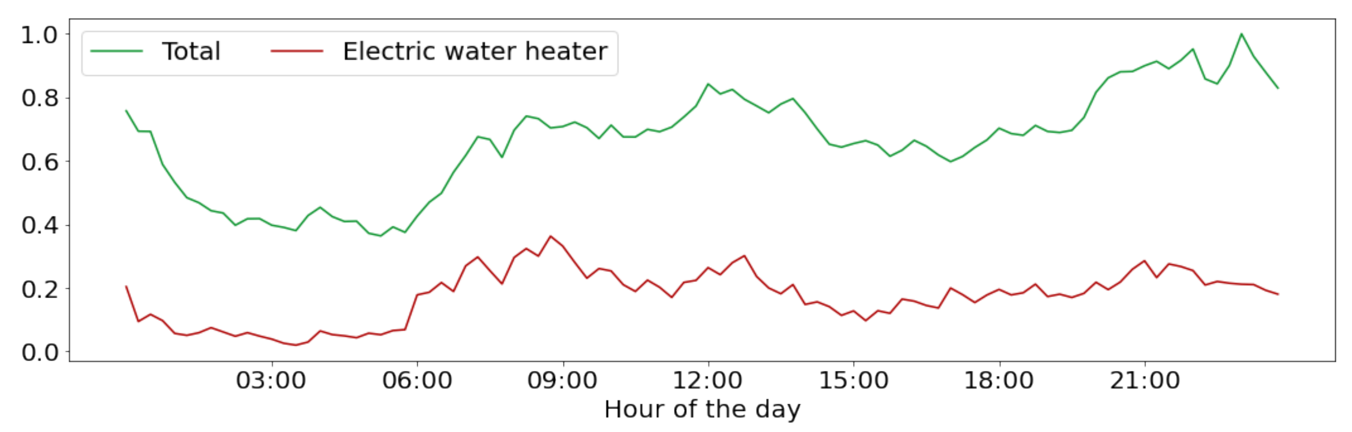
In most countries, the profile of total electricity consumption shows two pronounced peaks: early in the morning, before starting the working day, and near two hours after people return to their homes from work. Usually, the power consumption of electric water heaters has a high correlation with the total consumption: both present coincident peaks, as shown in Figure 1, for a representative analysis using data from the electric water heater consumption subset, part of the ECD-UY dataset. This correlation is explained by the high impact of water heaters compared with other domestic appliances. For example, in the case study analyzed in this article (Uruguay), water heaters account for 27% of the total residential electricity consumption, on average, peaking at 35%, according to the subset data. A specific feature of water heaters is that they have the ability to accumulate energy in the form of heat inside the water tank. This thermal inertia allows proper planning of switch on/switch off periods to help the grid operation while trying to affect the thermal comfort of users as little as possible.
According to the correlation between total energy consumption and water heaters’ energy consumption, the amount of energy associated with electric water heaters within a demand peak can be deferred by switching off the devices in a proper moment and switching them on in the future. This strategy allows implementing a load shifting on the demand curve, since the total amount of energy consumed in the period remains equal but the load profile is modified. Several studies have addressed the load shifting problem using direct control of devices [11,12], but few articles have focused on quantifying the thermal discomfort generated by the real application of this strategy.
2.3. Problem Formulation
The problem proposes determining an index for the quantitative evaluation of the discomfort generated by the application of load shifting using a direct control of electric water heaters. Two main challenges must be addressed to solve the problem: determining proper variables for the analysis and, since no-deterministic behavior is involved, proposing an effective methodology to estimate their values.
The first step is evaluating relevant variables for the problem. In the case of electric water heaters, the main variables affecting the comfort of the users is the temperature of the water in the tank and variables that determine the utilization pattern of water heaters. Regarding user comfort, installing a remote device to the water heater that allows measuring its power and switching it off or on is reasonable, since it can be achieved via specific Internet of Things controllers without modifying the water heater structure [13,14]. However, installing a remote thermometer to measure the temperature of the tank requires modifying the structure of the water heater, which implies a significant monetary investment. Thus, non-intrusive methods [15] are preferred for the analysis.
The main goal of defining a proper direct control strategy is to determine the discomfort introduced by the same controlling action among several electric water heaters to decide which of them intervene and minimize the probability of generating discomfort. Therefore, it is not crucial to compute the temperature exactly, but a good approximation is enough for analyzing differences. Another relevant aspect for the analysis is that the user perceives thermal discomfort only when using water and the temperature is below a given threshold. At any other time, or if the water temperature is still above the threshold despite the intervention, users are not aware of the switching-off actions.
Two variables must be estimated to define a discomfort index in the event of an intervention: the water utilization and the temperature of the water in the tank. By estimating these two variables, the proposed TDI takes into account the period of time that the water temperature is below the comfort temperature for a person using the water. This way, the proposed TDI properly models the human discomfort associated with an intervention.
3. Related Works
This section reviews relevant related works about load reduction techniques and thermal discomfort evaluation.
Several works in the literature have described the main concepts of peak load reduction strategies and specific implementations in smart grids [9,16]. In particular, direct load control allows utilities to remotely manage electricity demand by modifying the operation of end-use devices to perform load shifting [11,17]. A special type of devices to perform load shifting are thermostat-controlled appliances (TCA). The main feature of TCA is that they provide flexibility to select the desired temperature, i.e., the thermostat set point [18,19]. In addition, some TCAs can also store energy in the form of heat, providing a great advantage over non-storage appliances when performing load shifting strategies. This is the case of domestic electric water heaters, which are the focus of this article.
Nehrir et al. [20] proposed and analyzed an interactive demand-side management strategy for electric water heaters, but the research did not elaborate on specific aspects of thermal discomfort of users. A recent article by Xiang et al. [21] introduced a complex strategy to minimize thermal discomfort related with electric water heater control. The proposed strategy requires information to build a time-varied weight matrix based on detected utilization patterns of domestic electric water heaters. In turn, the weight matrix and other information are used to generate a customer satisfaction prediction index. Due to the large amount of information required to build the model, the approach is difficult to apply in practice.
Demand response control strategies for TCA can be effectively implemented provided that thermal comfort is not compromised. Thus, quantifying the impact on user comfort is a crucial aspect, and it has been the focus of several works. Kampelis et al. [22] evaluated the thermal discomfort in demand response control of several appliances used for heating, ventilation, and air conditioning in a university building. A daily discomfort score was proposed for demand response events to reduce the cost of energy, but the proposed strategy requires knowing the real temperature. Regarding electric water heaters, the study of the hot water utilization profile by end-users is a key aspect for estimating discomfort. Tabatabaei and Klein [23] studied whether a smart heating system can benefit from good predictions of the user behavior. Pirow et al. [24] proposed an algorithm for estimating domestic hot water utilization, but the technique requires the installation of temperature and vibration sensors.
The main factor that defines comfort is the water temperature. Thus, a model to estimate water temperature from measured information is crucial for the effectiveness of the comfort evaluation. Paull et al. [25] proposed a water heater model to estimate the temperature of the water in the tank as a function of time and the related variables, including the thermal losses and the water utilization. Data from smart meters, recorded at 15 min intervals, were used for validation. The model was proposed to be applied in a multiobjective demand-side management program. The study by Lutz et al. [26] provided a comprehensive empirical analysis of a simplified energy consumption model for water heaters considering the variation of the temperature of the water in the tank. Results of the proposed Water Heater Analysis Model (WHAM) model were compared with data from water heaters simulation programs (TANK, WATSIM, and WATSMPL). WHAM obtained very accurate prediction results, while being significantly faster. In addition, WHAM requires less detailed engineering information about the water heaters. Finally, comfort evaluation must be considered in the problem of controlling a subset of electric water heaters, e.g., by building a ranking to sort all interruptible devices according to appropriate criteria. Yin et al. [27] proposed a scheduling strategy based on a temperature state priority list. In turn, Al-Jabery et al. [28] analyzed a scheduling strategy for electric water heaters based on approximate dynamic programming techniques and q-learning.
The analysis of related works allows concluding that few articles have studied the thermal comfort effect when applying direct load control of electric water heaters. Existing approaches are based on installing specific sensors or devices to monitor water temperature or on building sophisticated algebraic formulations for modeling utilization patterns. This article contributes in this line of works by proposing an approach to evaluate the thermal discomfort of an intervention on electric water heaters, without requiring installing additional devices (e.g., a thermometer to measure the water temperature). Instead, the proposed model follows a non-intrusive approach, applying data analysis and computational intelligence and demonstrates its effectiveness on realistic problem instances.
4. The Proposed Approach for Defining a Discomfort Index
This section describes the proposed approach for defining a discomfort index for demand response via direct control of water heaters. The approach applies ideas described in the previous sections and follows a data analysis approach [29,30] considering inforation from a group of remotely controlled electric water heaters located in Uruguay.
4.1. Data Preparation
The data used in this article were provided by the Uruguayan National Electricity Company (UTE). Data are available in the “Electric water heater consumption” dataset, one of the three subsets included in EDC-UY [6], an effort to build a national database of energy consumption by gathering data from several households located in the main Uruguayan cities.
In this article, only the electric water heater consumption records were used. These records have a sample period of one minute and cover a date range from 2 July 2019 to 26 October 2020. Customer records were filtered by the recording length, keeping only those with more than 5 months of recording (i.e., at least 216,000 records).
The disaggregated electric water heater data have several gaps caused by different problems that arose during the data collection process (e.g., malfunctioning of the data transmission network, power failures, etc.). The gaps were filled using two techniques: resampling and refilling. The resampling technique normalizes the sample period to an exact minute. First, the records are grouped by customers to build one-minute record containers, starting from the date and time of the first record. Then, records whose date and time match with the date range of the container are assigned to it. In case one or more records match the same container, the minimum consumption value is set; otherwise, a null value is set (i.e., it corresponds to a missing record). The resulting data are taken as the input of the refilling technique. First, refilling detects the data gaps (i.e., consecutive missed records) and refills each one of them according to the following criteria. Starting from both extremes of the gap up to seven minutes forward/backwards, the missing data is recreated by a linear interpolation method. Finally, if missing values are still present at the gap (i.e., the gap is larger than 14 min), the null value is assigned to all missing values. The described process results in normalized time series of consumption values without gaps. For data preparation purposes, a Jupyter notebook was implemented, and the basis of the scripts was provided by the ECD-UY dataset. The Jupyter notebook uses Python (version 3) programming language and libraries Pandas and Numpy. The resulting notebook is available to download from https://bit.ly/3h133qu (accessed on 23 October 2021).
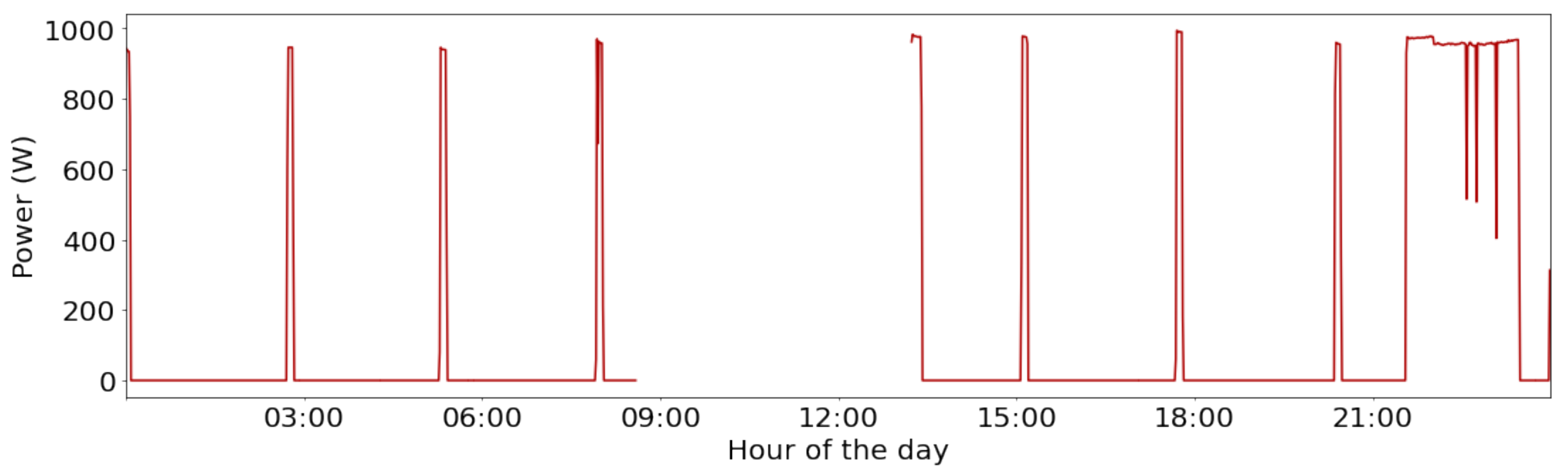
An example of the effects of the refilling procedure on electric water heater activations is presented in Figure 2 (missing records) and Figure 3 (after processing). Both figures show the same water heater activations in the same date and time range. The first graphic shows the dataset before refilling the gaps and include the missing records. The second graphic was captured after the data were processed.
4.2. Water Utilization Forecasting Model
4.2.1. Overall Description
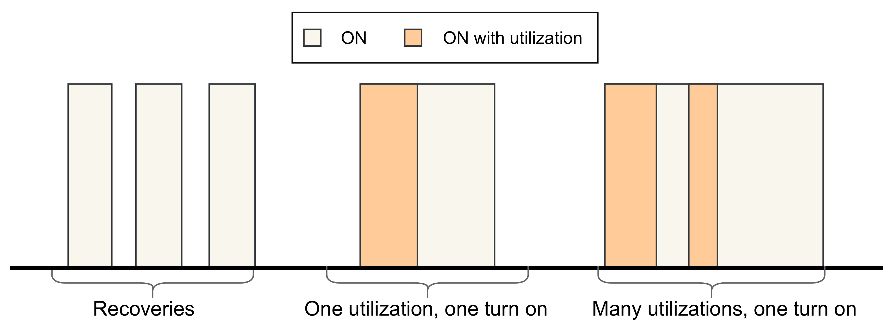
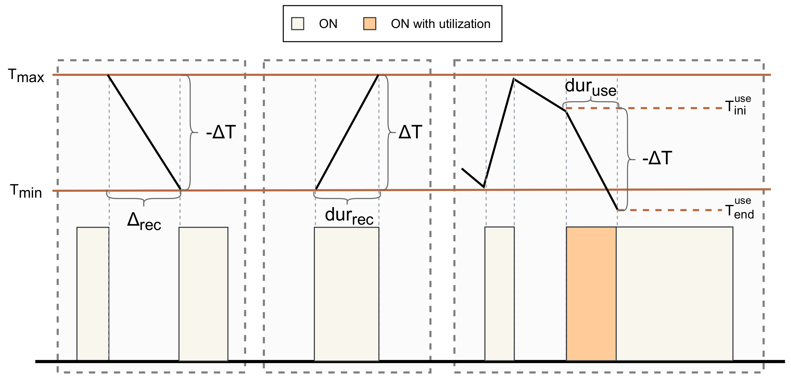
The proposed model for water utilization forecasting is based on a specific characteristic of electric water heaters: when this appliance is on, its power consumption can be considered as constant, since it just has slight variations. Therefore, the load curve of an electric water heater can be represented in a binary format (0 when the appliance is off and a given value C when the appliance is on). A pattern similarity approach [15] is proposed to estimate water utilization. To properly characterize the utilization patterns, let us define an on block as the time interval in which the electric water heater is switched on continuously. From the analysis of the power consumption time series, some of these on blocks are associated with water utilization by the user and other (shorter) on blocks correspond to thermal recoveries to maintain the target temperature of the water.
4.2.2. Methodology
The proposed forecasting model is based on identifying the on blocks associated with water utilization and discarding those corresponding to thermal recoveries. In this regard, a threshold duration is defined, and any on block shorter than the threshold duration is considered to be a thermal-recovery on block and not considered for the analysis. The proposed approach is robust, since discarding short blocks is not relevant for the main goal of identifying long-term utilization blocks, which are generally associated with showers. The analysis considers as a baseline an electric water heater with a capacity of 60 L and an average water outlet flow rate, which is representative of a highly efficient appliance. In fact, these electric water heaters are the main target of a campaign to promote energy efficiency in residential buildings in Uruguay. For an electric water heater with a capacity of 60 L, the empirical duration of an on block is on average eight times the duration of the utilization period. The proposed approximation is applied to convert the information about on blocks into an estimation of the water utilization by users. An example of the identified on blocks and the inferred water utilization patterns obtained with the aforementioned procedure is presented in Figure 4. In the analysis, the proposed model is applied to forecast the water utilization each minute in a period of two hours. Thus, the output of the model is a vector of 120 Boolean values, indicating the water utilization (or lack thereof) in each minute.
4.2.3. Formulation
The forecasting model for water utilization is based on an extremely randomized trees (ExtraTrees) regression model. ExtraTrees is an ensemble learning method for solving classification and regression problems that operates as a Random Forest (RF) technique. ExtraTrees defines a set of decision trees that is trained with training data, and the resulting output class (for classification problems) or prediction (for regression problems) is defined as the mode (for classification) or mean/average prediction (for regression) of the considered decision trees [31]. Using a large number of trees allows properly dealing with overfitting problems that arise when using few trees. ExtraTrees has two main differences with the standard procedure defined by RF: (i) each tree is trained using all the training data (and not using just a bootstrap sample, as the standard RF method), and (ii) a further step of randomization is included in the top-down splitting in the tree learner by selecting a random cut point for each considered feature in the problem (according to a uniform empirical distribution to select between the values for each feature in the training set). The split that computes the best result is then used to split the considered node of the tree [32]. ExtraTrees have proven to be an accurate predictor for electricity-related problems (e.g., for demand forecasting in industrial and residential facilities [7]).
Input features considered for the proposed ExtraTrees regression method include:
- Use (, 120 Boolean values): indicating whether a water utilization occurs in the past 120 min.
- Month (m, integer): indicating the month of the horizon to forecast.
- Day (d, integer): indicating the day of the horizon to forecast.
- Hour (h, integer): indicating the hour of the horizon to forecast.
- Dayofweek (, integer): indicating the day of the horizon to forecast.
- Workingday (, Boolean): indicating if the horizon to forecast is a working day or not.
Fine-tuning of the proposed ExtraTrees regression method was performed using grid search techniques for hyperparameter settings. Hyperparameters are external parameters, inherent to the learning model, whose values cannot be set or estimated from training data. Hyperparameter values affect the quality of the resulting model, and appropriate values must be set before launching the learning process. Grid search techniques define a search space as a grid of different combinations of candidate hyperparameter values and proceed to evaluate every combination in the grid. In this article, the GridSearchCV method from scikit-learn was used. GridSearchCV (the CV stands for cross validation) was applied with varying parameters: number of estimators and max tree depth, considering 10-folds cross-validation and the predetermined evaluation metrics over the model. After the model is trained, a vector with 120 Boolean values (), representing the water utilization forecast for the next two hours, is obtained according to the Equation: .
4.3. Water Temperature Model
4.3.1. Overall Description
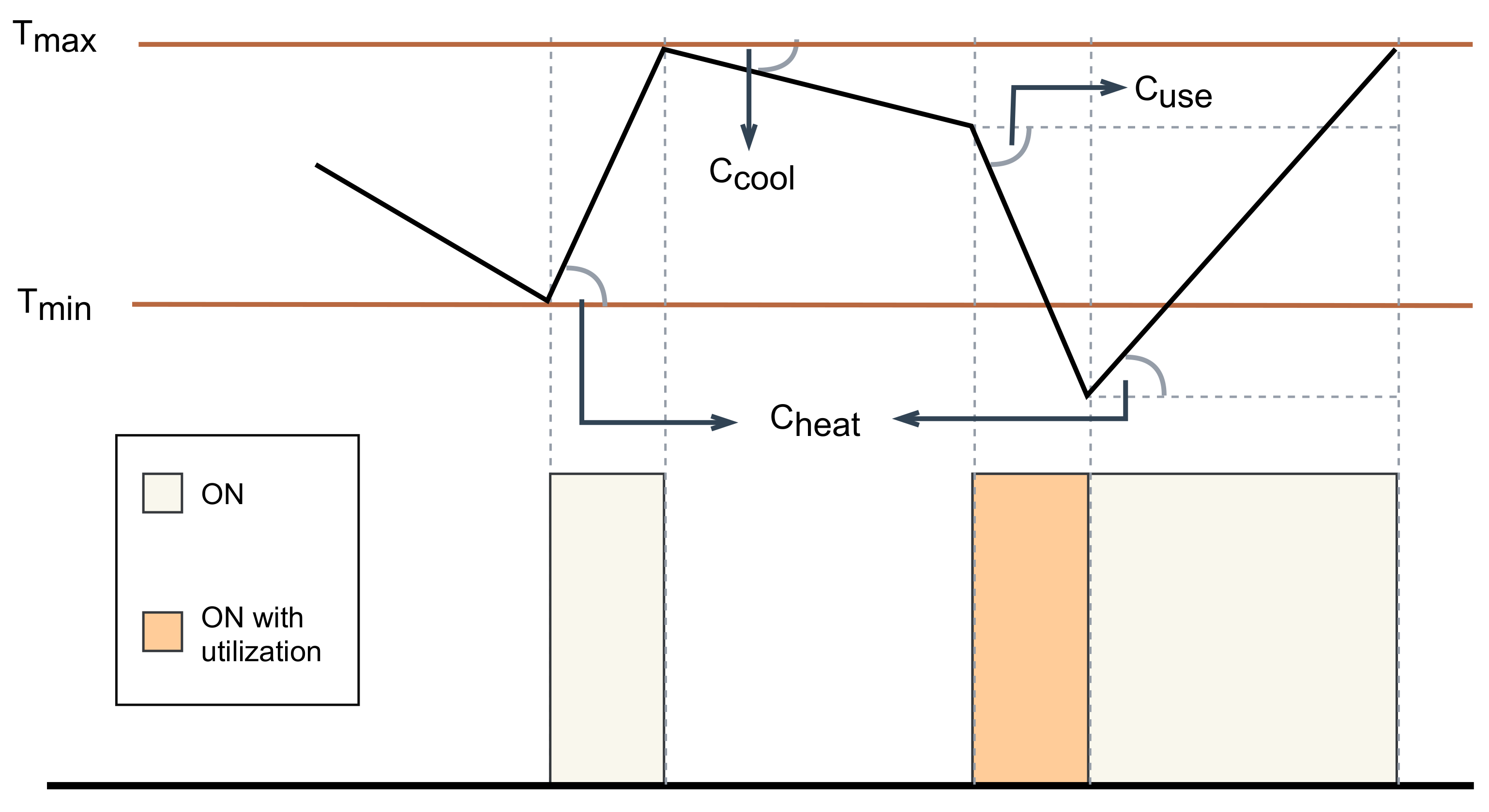
The general formulation of equations for heating and cooling water in thermal tank devices, such as water heaters for domestic use, include a large number of variables. Existing models, even when they simplify the formulations, depend on several variables, including the insulation factor, the ambient temperature, the flow of water used, the time of use, and the tank volume, among other factors [26]. To overcome the difficulties of knowing beforehand all these variables, which are often difficult to determine in practice, the pattern similarity approach proposed for estimating water utilization is applied to define a linear temperature model, which provides a good approximation in order to estimate the TDI. The linear model provides a reasonable approximation, since the cooling and heating curves in this model are straight lines.
Five parameters are defined to build the temperature model from gathered data about on blocks and water utilization:
- is the temperature at which the electric water heater is turned on by the action of the thermostat when the water is cooling.
- is the temperature at which the electric water heater is turned off by the action of the thermostat when the water is heating.
- is the slope of the line when the electric water heater is turned on.
- is the slope of the line when the electric water heater is turned off and no water is being used.
- is the slope of the line when using water, whether or not water is being used.
The considered parameters depend on several factors. In this article, a specific approach is proposed to compute a robust approximation for each parameter value, i.e., to guarantee that all possible temperature approximation errors always produce underestimated temperature values. Thus, the proposed model is conservative about comfort estimation, in order to not affect the quality of service provided to the user.
The model assumes that the user sets the thermostat at a temperature value of 60°, which is the suggested temperature not only to achieve energy efficiency in households, but also due to health concerns, such as avoiding the proliferation of Legionella bacteria [33,34]. Without loss of generality, the variation range defined by and is considered. In any case, the proposed model is fully extensible to work with other values of and . The use of this model in an industrial context should consider: (i) variations in the set point of the thermostat (e.g., values extracted from statistics or provided by the users via survey or web/mobile application), and (ii) variations in the temperature of the room, in the average water utilization, and in the temperature of supplied water. Variations are captured by recomputing the coefficients after variations occur. Since the model is estimated from on-and-off data of the water heater in real time, the variations of and should be updated frequently. After that, coefficients , , and should be recomputed using the updated values of and . These dynamics allow properly modeling different climate conditions and user preferences.
Figure 5 presents a schema of the proposed model definition from on blocks and water utilization. The black line on the upper graphic is the water temperature. On the bottom, grey on blocks represents thermal recoveries, and on blocks caused by water utilization are marked in orange. The analysis of the water temperature curve indicates that the water cools with a slope until it reaches the value ; at that moment, the electric water heater turns on. The heating phase starts with a slope until the temperature reaches the value . Then, another cooling phase occurs until a water utilization causes a much faster cooling with a slope . During the water utilization, the electric water heater turns on almost immediately after opening the water stream. When the water utilization ends, the electric water heater remains on because the water temperature is below , so it heats the water with a slope until temperature is reached, where the gray on block ends. Assuming the described behavior, an algebraic approach can be applied to compute the three slopes.
The described procedure allows computing an approximation of the water temperature in a given interval from a set of on blocks and water utilization data in that interval. Therefore, a temperature forecast can be obtained from a set of on blocks predicted for a future time interval. The forecasting method can be applied to other situations, e.g., to simulate a remote switch off of the electric water heater, associated with a demand response action, and obtain the water temperature forecast for this event.
4.3.2. Formulation
The linear temperature model is applied to determine the values of coefficients , , and . The input data for the temperature model are the values of and and the information about on blocks and water utilization.
The coefficients of the model are calculated as follows:
- Coefficient . First, two consecutive temperature recoveries are identified. Then, is calculated as the time between the the end of the first recovery and the beginning of the next recovery. Finally, is calculated by Equation (1). The procedure is described in the left box of Figure 6. From the graphic, .
- Coefficient . The first step is identifying a temperature recovery followed by a water utilization event. Then, and are defined as the temperature at the beginning and end of the utilization, respectively. To compute , the value of (already computed) is used as the slope to draw the line that passes through at the end of the recovery, and intersects with the start of the utilization. Similarly, to compute , the value of (already computed) is used as the slope to draw the line that passes through the end of the on block associated with the utilization and intersects with the end of the utilization. is defined as the duration of the utilization. Finally, is calculated by Equation (3). The procedure is described in the right box of Figure 6.
4.4. Defining the Thermal Discomfort Index
The proposed index is conceived to capture the thermal impact that a user suffers due to an intervention by the electrical company in the electric water heater. The TDI is defined using the defined water use forecasting model and the temperature model. Since every forecast has uncertainty, the index is defined in terms of the expected value of the difference of the aforementioned temperatures, as expressed by Equations (4) and (5).
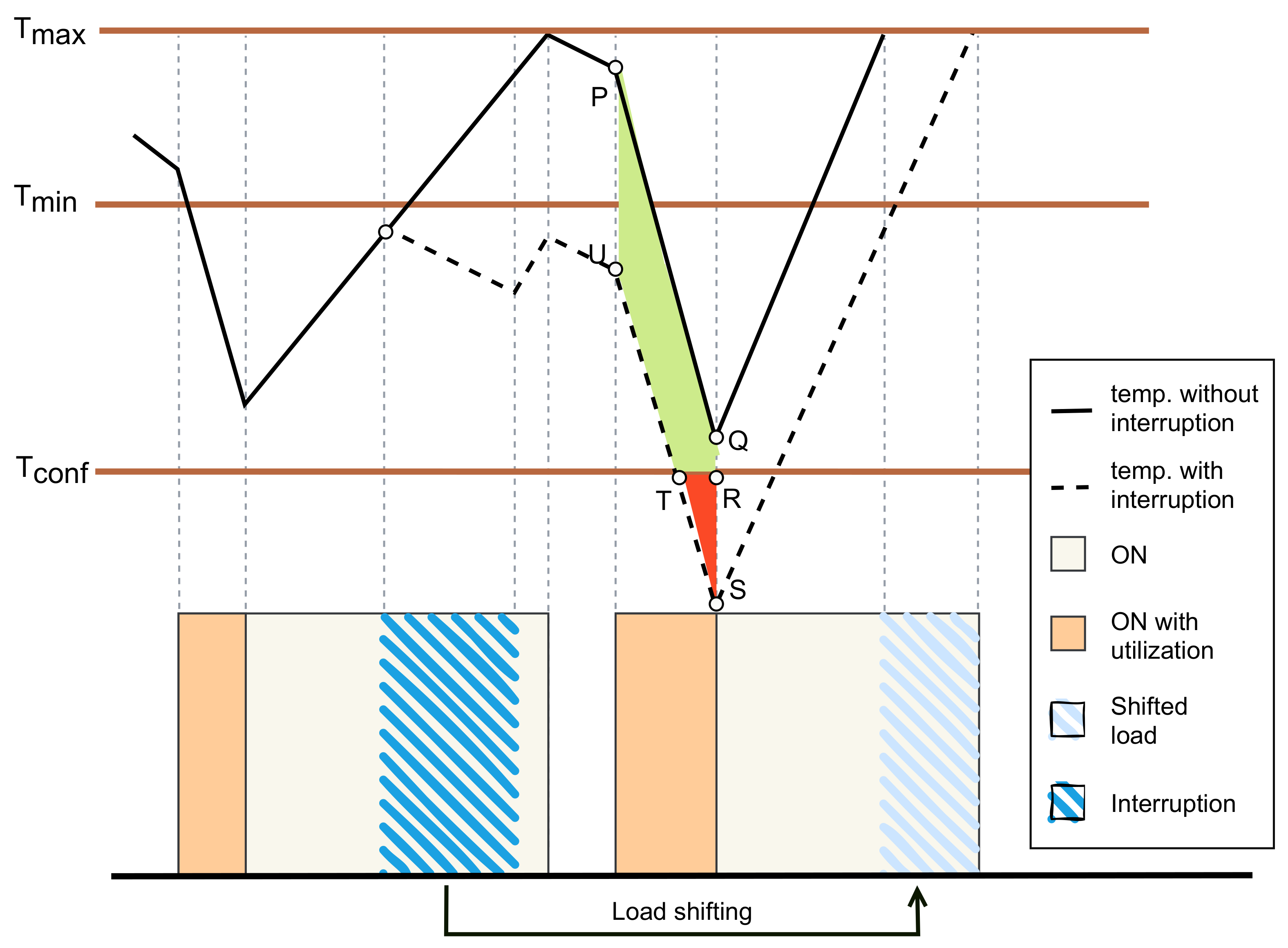
In Equation (4), represents the discomfort index of an interruption I, a water utilization u, and a realization w that defines a single scenario of water use and temperature evolution. The values and are the starting and finishing time of utilization u. For every realization w, is the temperature curve without interruption and is the temperature curve with interruption. Both curves are obtained using the temperature model described in Section 4.3 for the realization w.
Finally, is the lowest water temperature that does not produce discomfort to the users, and represents the time interval in which ≤ . The value is a parameter that acts as a penalty over the area below the comfort temperature.
In Equation (5), I denotes the interruption of the electric water heater by the electric company. In turn, ] represents the expected value of the expression inside parenthesis with respect to the random variable w. Each realization of the random variable w generates a different forecast of water use. Therefore, a forecast of the temperature obtained using the model described in Section 4.3 is also generated. U(w) is the set of water utilization intervals in the analyzed time horizon associated with the forecast generated by w.
Figure 7 presents a visual representation of . Two temperature curves are represented on the upper graphic. The full black line represents the water temperature when no interruption occurs. In turn, the dotted black line represents the water temperature when an interruption occurs at time . The green area between the curve of water temperature without interruption and the curve of water temperature with interruption (defined by the polygon PQRTU) is computed by the integral . This area represents the heat loss due to the interruption. In turn, the red area below the comfort temperature (defined by the polygon RST) is computed by the integral and weighted by the penalty . Introducing the penalty term is interesting to provide the model the flexibility for adjusting the weight of the red area below the comfort temperature with respect to the whole area of temperature reduction (PQSU).
The expected value of TDI, as defined in Equation (4), is computed by applying a Monte Carlo (MC) simulation method. First, the MC method samples 100 realizations of the value w, with a normal distribution . Then, for each value of w, the following procedure is applied:
- The next 12 h are forecasted using the model described in Section 4.2. Six iterations are applied, considering that the Extra Trees regressor is defined for a period of two hours (120 observations).
- Using the temperature model described in Section 4.3 and the water utilization forecast, the water temperature is obtained for the next 12 h.
- An interruption of k minutes is simulated and the temperature for the next 12 h is obtained using the proposed temperature model.
- Since , , are known, Equation (5) is applied to compute for the current realization w and all uses.
- An auxiliary variable is defined by Equation (6).
Finally, after computing for each realization, TDI is computed as the empirical expected value defined in Equation (7).
5. Experimental Validation
This section presents the experimental validation of the proposed approach for defining a TDI.
5.1. Methodology
The methodology for the experimental evaluation includes two steps: validation of forecasting models and validation of the proposed index.
5.1.1. Validation of Forecasting Models
The first step of the experimental evaluation consists of validating the two models required to calculate the TDI (water utilization forecasting and water temperature). For the validation of the aforementioned models, the standard mean absolute percentage error (MAPE) metric is used to evaluate the forecasting capabilities. MAPE is defined in Equation (8), where represents the measured value for , represents the predicted value, and n is the predicted horizon length.
5.1.2. Validation of the Proposed TDI
After determining the forecasting accuracy of the proposed models, the second step of the experimental evaluation consists of validating the TDI calculation and utilization in realistic scenarios in order to properly evaluate the thermal discomfort of users. For this purpose, three experiments were designed based on scenarios that adequately represent the real operation of water heaters. A water heater dynamic simulator was developed and used to generate real scenarios. The description of the simulator and the experiments performed are presented in Section 6.
5.2. Development and Execution Platforms
Data processing algorithms and the proposed models to build the TDI were implemented using Python and well-known open source libraries such as Pandas, Numpy and Tensorflow. Data processing and the experimental analysis were performed on the high performance platform of National Supercomputing Center (Cluster-UY), Uruguay [35].
5.3. Evaluation of the Water Utilization Forecasting
Metrics defined in Section 4.2 were applied to evaluate the implementation of the water utilization forecasting model. A subset of ECD-UY was used, consisting of ten electric water heaters with more than five months of measurements. The grid search was performed on a two-dimensional grid to determine the best values for the number of trees in the forest and the maximum depth of the tree. The best parameter setting found applying the grid search configuration was n_estimators = 50, max_depth = 200.
Using the best parameter configuration, the ExtraTrees regressor achieved a MAPE value of 11.79 in just 4.09 s of execution time. This accuracy is adequate for estimation purposes to compute TDI, considering the high variance of individual water utilization. The method is useful for generating scenarios to apply the Monte Carlo simulation approach in order to estimate the empirical probability distribution of water utilization.
5.4. Evaluation of the Water Temperature Model
The linear model described in Section 4.3 was evaluated for a real case study corresponding to an electric water heater with a thermometer to measure the temperature of the water in the tank. The defined setting of the thermostat allowed knowing in advance the values of parameters and . The corresponding values are and . Then, the other parameters of the model were calculated as described in Section 5.3. Finally, data of twelve hours on blocks of the electric water heater were used to estimate the temperature and compared with the real temperature measured. Table 1 reports the comparison of the real and the estimated temperature, and the largest difference in the three long utilization periods in the twelve hours analyzed.
The second utilization had the largest temperature difference ( , marked in light blue in Table 1), which represents a percentage error of in the worst case. The other utilizations had a significantly lower error. The accuracy of the temperature model is adequate for the purpose of estimating TDI.
6. Application of the Proposed Model: TDI Calculation
This section describes the application of the proposed model for TDI calculation over relevant sample scenarios.
6.1. Overall Description
The main challenge when designing the TDI was to properly capture the differences between demand response strategies in order to fairly select water heaters to interrupt while minimizing the discomfort of users. Therefore, evaluating the TDI calculation is important to have real scenarios that capture the utilization profile of the users of electric water heaters. Evaluating the proposed methodology over a real scenario is not an easy task. The scenario must include a set of real water heaters large enough to carry out experiments on real water uses, and real interventions must be set up. To overcome these difficulties, a common approach in the related literature [22,26] consists of using simulations of thermal appliances.
A simulator was implemented to perform the experimental evaluation in those scenarios where real data is not available. The consists of two modules: the individual water heater module simulates the energy dynamics of a water heater, based on the work by Lutz [26] and the household utilization module generates scenarios of water utilization for a group of households, using a vector of hourly probabilities of water usage as input.
The proposed TDI is evaluated in three different scenarios accounting for different number of water heaters, households, and priorities. Scenario #1 considers two water heaters and real data for both temperature and the electrical state (ON/OFF) of the water heaters. Scenarios #2 and #3 considers a large number of water heaters, for which real data about the electrical state are available. In turn, the developed temperature and water utilization models, implemented in the simulator, were applied to validate the proposed TDI. The main details of the evaluation are reported in the following subsections.
6.2. Scenario #1: Evaluation of a Simple Case Study with Two Real Water Heaters
One of the main challenges related to the definition of TDI is modeling the differences of temperature (, a quantitative factor) between performing an interruption in different moments. A relevant case is analyzing the values situations in the interruption affects the most to comfort.
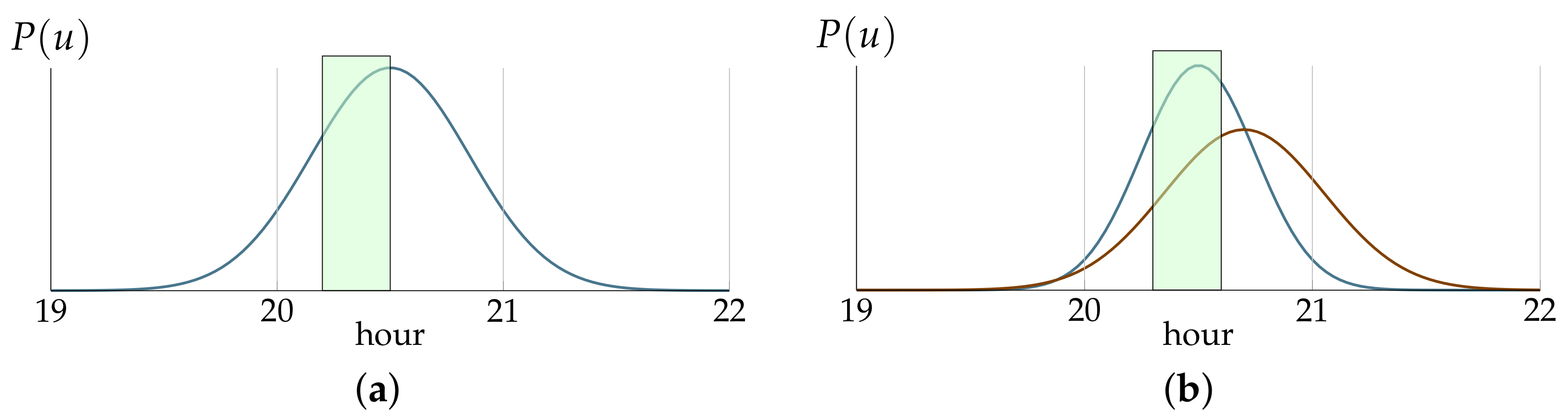
As a relevant sample study, the comparison of the TDI for two different values of and two particular electric water heaters ( and ) is presented. The considered electric water heaters model two different utilization patterns from two different users. On weekdays, has two consecutive utilizations, and is only used once. The TDI associated with a 20 min interruption between 20:10 and 20:30 was considered for this case. Figure 8 presents the empirical distribution of uses () from 19:00 to 22:00 for (left) and (right). For each case, the interruption period is represented by a green band.
For the presented example, it is expected for the TDI value to be higher for than for , because in the hours immediately after the interruption analyzed, the average historical utilization is higher for . On the other hand, as the value of increases, it is expected that the gap between the TDI of both electric water heaters becomes larger. Table 2 reports the TDI values computed for each electric water heater, considering two different values of (, and ).
The results in Table 2 confirm that the proposed index correctly models discomfort. The TDI value is higher for , and the difference widens when considering larger penalty values (). Results show that TDI properly models the differences of temperature between a scenario with an interruption and a scenario without interruption, as expected.
6.3. Scenario #2: Evaluation on a Group of Households with Water Heaters
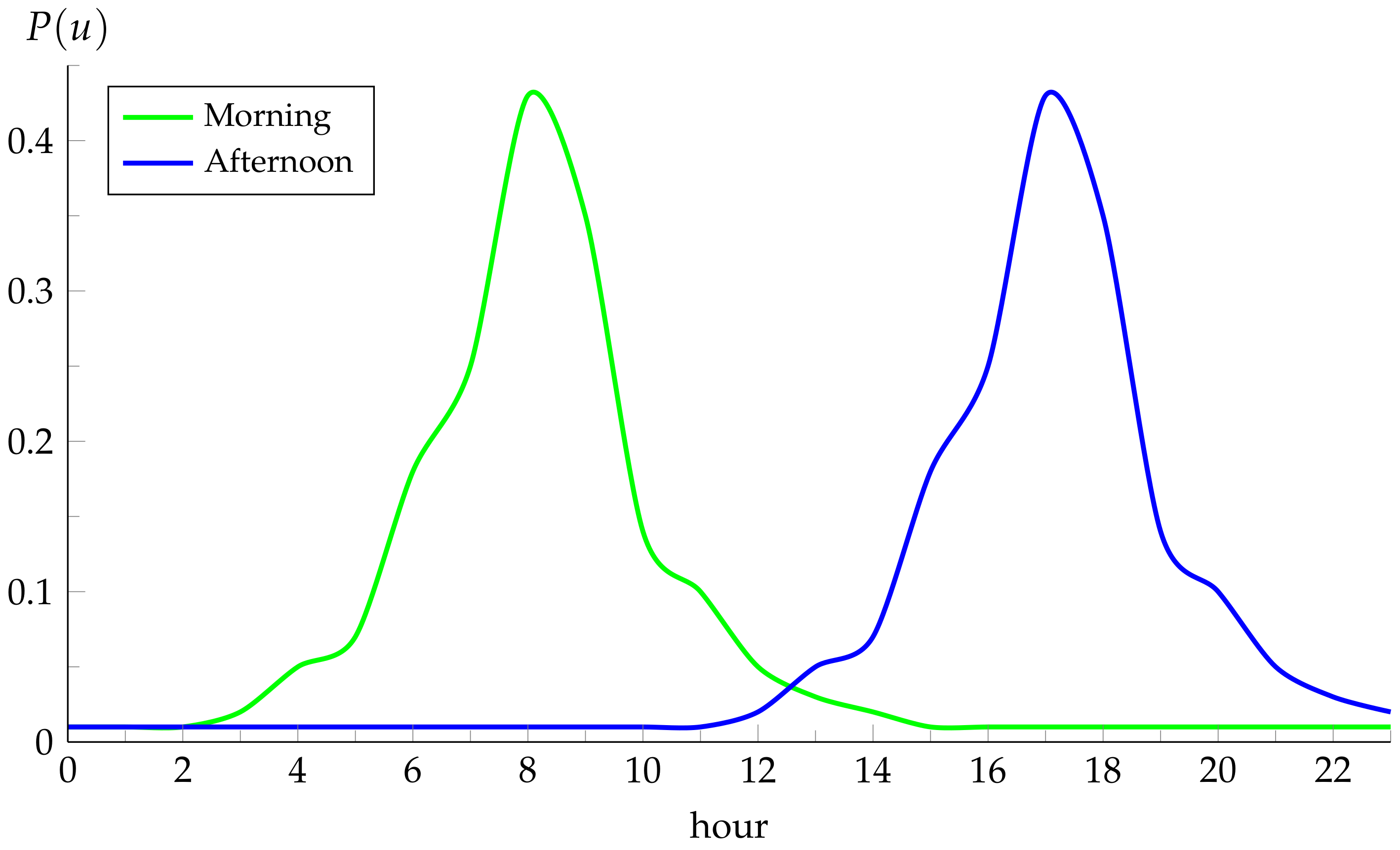
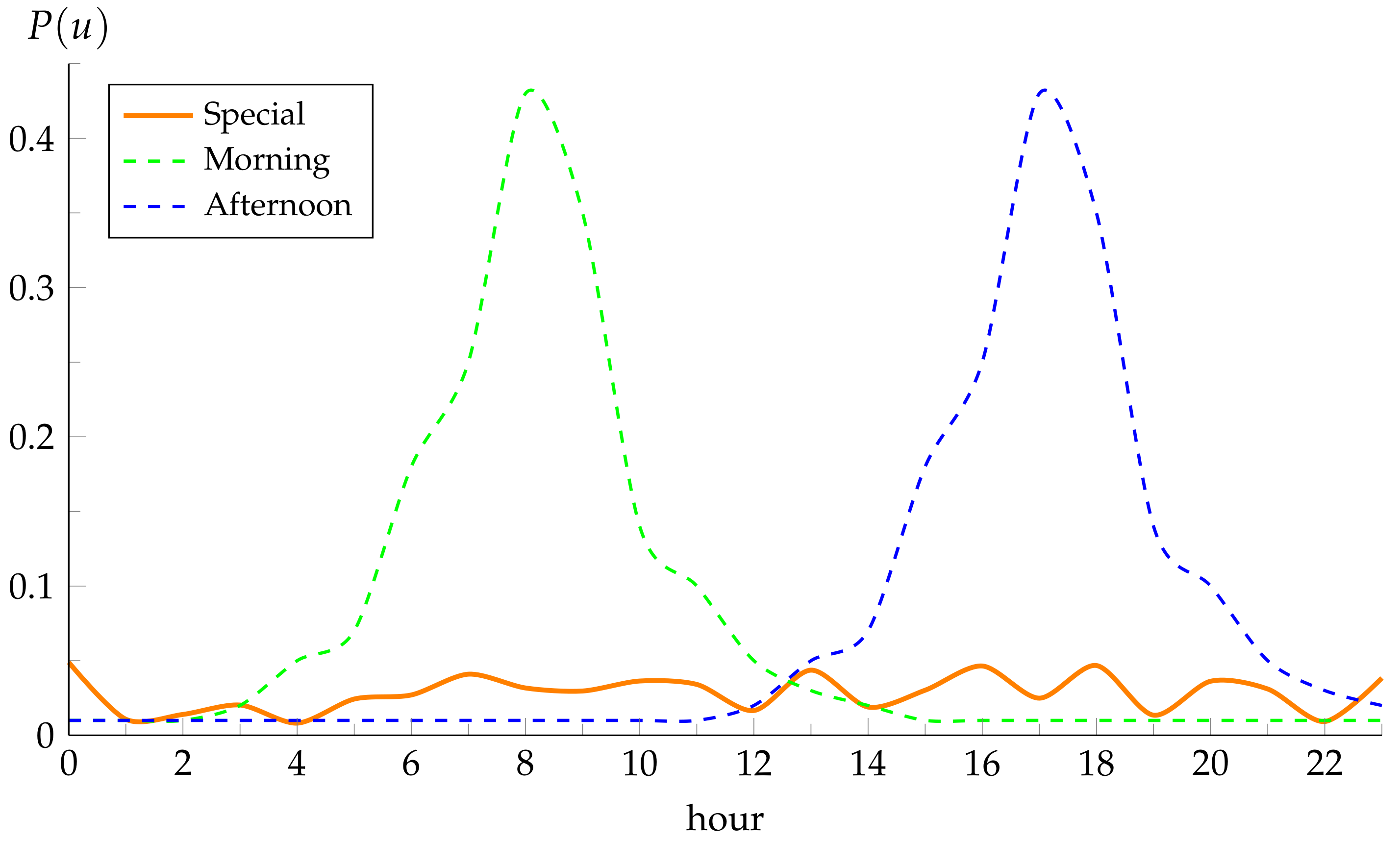
Another challenge related to the definition of TDI is to prioritize which group of water heaters should be interrupted to reduce electricity demand while minimizing discomfort (e.g., for demand response management in a peak situation). In this experiment, a group of twenty households H with electric water heaters was studied using the developed simulator. Ten households () have a water use profile concentrated in the morning hours and the other ten households () in the evening hours. Figure 9 presents the average water use profiles for each type of household.
A simulation of a complete day for the twenty defined households was performed. In turn, the TDI associated with a 20 min interruption between 7:10 and 7:30 () and the TDI associated with a 20 min interruption between 20:10 and 20:30 () were computed for the twenty households using the method presented in Section 4.4.
Table 3 reports the computed TDI values for each household. Table 4 presents the two rankings defined: Ranking sorts households according to the values of and Ranking sorts households according to the values of , both from lowest to higher values. households are highlighted in green and in blue.
For the presented case study, and considering that the probability of affecting comfort when interrupting water heaters in the morning is higher for households H1, ..., H10 these ten households are expected to be in the last ten positions of Rankingm. Analogously, H11, ..., H20 are expected to be in the last ten positions of Rankinga. Results in Table 4 confirm that the TDI properly sorts the water heaters according to the real discomfort produced for users, as expected. These results allow for very precise information to decide about specific demand-management interventions.
6.4. Scenario #3: Setting ρ to Tune the Interruption Priority of a Special Water Heater
In several circumstances, an electric water heater is installed with specific objectives and should not be considered to be interrupted in a demand-management event. An example of this situation is a nursing home, where hot water is used for sanitary purposes. A simple approach to deal with this scenario is excluding the electric water heater from the list of appliances to be interrupted by the energy utility. This approach is not flexible because it only allows inserting or removing a device from the interruptible list and does not allow prioritizing special appliances. However, using the proposed TDI definition, the parameter ρ is used to independently weight those special electric water heaters. In this experiment, the case presented in Section 6.3 is extended by adding a household (HE) with an special water heater. The hypothesis of the experiment is that the special water heater in household HE has a water use profile almost constant throughout the day, and it cannot be interrupted in demand-response events. Figure 10 shows in orange the hourly probability vector of this special water heater. Green and blue dotted lines correspond to the profiles of households with water use concentrated in the morning and in the evening, respectively. The experiment consists of adding the device with the same value of the parameter ρ = 1 used in the base experiment and calculating Rankingm and Rankinga. Then, the value of the parameter ρ for the special device is set to a very large value (ρ = 1000), and differences are analyzed.
The proposed scenario was studied via simulations. Two special household values were included, using ρ = 1 and using ρ = 1000. Table 5 reports the TDI values obtained in the simulations, considering the two special households (highlighted in red) and highlighted in orange). Table 6 reports the order defined by Rankingm and Rankinga considering , and Table 7 reports the order defined by Rankingm and Rankinga considering .
Results reported in Table 6 demonstrate that the special electric water heater isnot ranked at the end of either Rankingm or Rankinga. A different situation is observed in the results reported in Table 7, which indicate that using the value ρ = 1000 only for the special electric water heater , this appliance appears last in both rankings Rankingm and Rankinga, as expected.
Overall, results obtained for scenario #3 validate the proposed approach and confirm the effect of modifying the ρ parameter for some water heaters to allow flexible demand-response strategies to be designed. For instance, a possible strategy is to define a classification of the complete set of households in three classes and associate each class with a different ρ value to define water heaters that are not interruptible, interruptible if necessary, and no restrictions for interruption.. The flexibility of the proposed TDI using different values of ρ facilitates, in a real scenario that is continually changing in structure, performing active demand management to quickly adapt to the needs of the electrical system.
7. Conclusions and Future Work
This article presented an approach to evaluate the impact on the thermal comfort of direct demand response control using electric water heaters. An index associated with the thermal discomfort was defined according to the following procedure. First, a water utilization forecasting model was built using real power data from a set of electric water heaters and applying an ensemble learning technique. Then, a linear model was developed to estimate the temperature of the water in the electric water heater tank. Finally, the TDI associated with an intervention on the electric water heater was defined stochastically, and calculated via Monte Carlo simulation. A specific water heater simulator was developed for the evaluation of the proposed TDI.
The computational models and the reliability of the proposed index were evaluated in three real case studies. The first case considered two electric water heaters from different users with different average historical utilization. The TDI values were analyzed for both electric water heaters for different penalization factors ρ. Results confirmed that the proposed index correctly models discomfort since higher TDI values were computed for the electric water heater with the higher average historical utilization. The difference in TDI values increased when considering larger penalty values. The second case analyzed the use of TDI for sorting water heaters according to the discomfort caused by their intervention. Two sets of ten households were generated and simulated, considering two different utilization patterns and two interruptions (in the morning and the evening). Results confirmed that in the ranking generated with the TDI computed for the morning interruption, households with high probability of water utilization in the morning were in the last ten positions of the ranking. A similar result was obtained for the afternoon interruption, as expected. The third case study explored the use of parameter ρ to tune the interruption priority, considering an additional special household and two values of ρ. Results demonstrated that the new special household was in eleventh position in both rankings when ρ = 1 and changed to the last position in both rankings when ρ = 1000, properly modeling a non-interruptible appliance (e.g., for sanitary reasons). The main lines of future work are related to estimating an economic value of the TDI index (in USD/MWh), useful to characterize the profit of reducing the energy demanded by a set of electric water heaters by applying the interruption action in order to compare this strategy with other demand response techniques (e.g., using fuel generators or batteries). Expanding the developed simulator to consider all generators in the system is another line for future work to fairly compare demand response strategies by using TDI values and the economic impact of an interruption.
Author Contributions
R.P.: research conceptualization, data analysis, code development, manuscript writing, manuscript revision and correction. J.C.: data analysis, data cleansing, manuscript writing, manuscript revision and correction. S.N.: research conceptualization, data analysis, manuscript writing, manuscript revision and correction. All authors have read and agreed to the published version of the manuscript.
Funding
This research received no external funding.
Institutional Review Board Statement
Not applicable.
Informed Consent Statement
Not applicable.
Acknowledgments
The work of S. Nesmachnow was partly supported by ANII and PEDECIBA, Uruguay.
Conflicts of Interest
The author declares no conflict of interest.
References
- Momoh, J. Smart Grid: Fundamentals of Design and Analysis; Wiley-IEEE Press: Hoboken, NJ, USA, 2012. [Google Scholar]
- Assessment of Demand Response & Advanced Metering; Technical Report AD-06-2-00; Federal Energy Regulatory Commission: Washington, DC, USA, 2006.
- European Automotive Research Partner Association. Smart Grids European Technology Platform. Available online: https://www.etip-snet.eu/ (accessed on 21 January 2021).
- Bhattacharyya, S. Energy Demand Management. In Energy Economics; Springer: London, UK, 2011; pp. 135–160. [Google Scholar]
- Instituto Nacional de Estadística, Uruguay. Microdatos de la Encuesta Continua de Hogares. 2019. Available online: http://www.ine.gub.uy/microdatos (accessed on 17 August 2020).
- Chavat, J.; Nesmachnow, S.; Graneri, J.; Alvez, G. ECD-UY: Detailed household electricity consumption dataset of Uruguay. Sci. Data 2020, submitted. [Google Scholar]
- Porteiro, R.; Nesmachnow, S.; Hernández-Callejo, L. (Eds.) Electricity demand forecasting in industrial and residential facilities using ensemble machine learning. Rev. Fac. Ing. Univ. Antioq. 2020, 102, 9–25. [Google Scholar]
- Deng, R.; Yang, Z.; Chow, M.; Chen, J. A Survey on Demand Response in Smart Grids: Mathematical Models and Approaches. IEEE Trans. Ind. Inform. 2015, 11, 570–582. [Google Scholar] [CrossRef]
- Hassan, N.U.; Khalid, Y.I.; Yuen, C.; Tushar, W. Customer engagement plans for peak load reduction in residential smart grids. IEEE Trans. Smart Grid 2015, 6, 3029–3041. [Google Scholar] [CrossRef] [Green Version]
- Tang, R.; Wang, S.; Yan, C. A direct load control strategy of centralized air-conditioning systems for building fast demand response to urgent requests of smart grids. Autom. Constr. 2018, 87, 74–83. [Google Scholar] [CrossRef]
- Ozoh, P.; Apperley, M.; Olayiwola, M. Modelling of household power consumption and its effects on load shifting strategies. J. Sci. Arts 2018, 18, 1067–1072. [Google Scholar]
- Witherden, M.; Rayudu, R.; Tyler, C.; Seah, W. Managing peak demand using direct load monitoring and control. In Proceedings of the Australasian Universities Power Engineering Conference, Hobart, TAS, Australia, 29 September–3 October 2013; pp. 1–6. [Google Scholar]
- Orsi, E.; Nesmachnow, S. Smart home energy planning using IoT and the cloud. In Proceedings of the IEEE URUCON, Montevideo, Uruguay, 23–25 October 2017. [Google Scholar]
- Orsi, E.; Nesmachnow, S. IoT for smart home energy planning. In Proceedings of the XXIII Congreso Argentino de Ciencias de la Computación, La Plata, Argentina, 9–13 October 2017; pp. 1091–1100. [Google Scholar]
- Chavat, J.P.; Nesmachnow, S.; Graneri, J. Non-intrusive energy disaggregation by detecting similarities in consumption patterns. Rev. Fac. Ing. Univ. Antioq. 2020, 98, 27–46. [Google Scholar] [CrossRef]
- Yoon, A.; Kang, H.; Moon, S. Optimal Price Based Demand Response of HVAC Systems in Commercial Buildings Considering Peak Load Reduction. Energies 2020, 13, 862. [Google Scholar] [CrossRef] [Green Version]
- Huang, D.; Billinton, R. Effects of load sector demand side management applications in generating capacity adequacy assessment. IEEE Trans. Power Syst. 2011, 27, 335–343. [Google Scholar] [CrossRef]
- Lu, N.; Katipamula, S. Control strategies of thermostatically controlled appliances in a competitive electricity market. In Proceedings of the IEEE Power Engineering Society General Meeting, San Francisco, CA, USA, 16 June 2005; pp. 202–207. [Google Scholar]
- Perfumo, C.; Braslavsky, J.H.; Ward, J. Model-based estimation of energy savings in load control events for thermostatically controlled loads. IEEE Trans. Smart Grid 2014, 5, 1410–1420. [Google Scholar] [CrossRef] [Green Version]
- Nehrir, M.; LaMeres, B.; Gerez, V. A customer-interactive electric water heater demand-side management strategy using fuzzy logic. In Proceedings of the Winter Meeting IEEE Power Engineering Society, New York, NY, USA, 31 January–4 February 1999; Volume 1, pp. 433–436. [Google Scholar]
- Xiang, S.; Chang, L.; Cao, B.; He, Y.; Zhang, C. A Novel Domestic Electric Water Heater Control Method. IEEE Trans. Smart Grid 2019, 11, 3246–3256. [Google Scholar] [CrossRef]
- Kampelis, N.; Ferrante, A.; Kolokotsa, D.; Gobakis, K.; Standardi, L.; Cristalli, C. Thermal comfort evaluation in HVAC Demand Response control. Energy Procedia 2017, 134, 675–682. [Google Scholar] [CrossRef]
- Tabatabaei, S.; Klein, M. The role of knowledge about user behaviour in demand response management of domestic hot water usage. Energy Effic. 2018, 11, 1797–1809. [Google Scholar] [CrossRef] [Green Version]
- Pirow, N.; Louw, T.; Booysen, M. Non-invasive estimation of domestic hot water usage with temperature and vibration sensors. Flow Meas. Instrum. 2018, 63, 1–7. [Google Scholar] [CrossRef] [Green Version]
- Paull, L.; MacKay, D.; Li, H.; Chang, L. Awater heater model for increased power system efficiency. In Proceedings of the Canadian Conference on Electrical and Computer Engineering, St. John’s, NL, Canada, 3–6 May 2009. [Google Scholar]
- Lutz, J.; Whitehead, C.; Lekov, A.; Winiarski, D.; Rosenquist, G. WHAM: A Simplified Energy Consumption Equation for Water Heaters; American Council for and Energy-Efficient Economy Summer Study on Energy Efficiency in Buildings: Washington, DC, USA, 1998. [Google Scholar]
- Yin, Z.; Che, Y.; Li, D.; Liu, H.; Yu, D. Optimal scheduling strategy for domestic electric water heaters based on the temperature state priority list. Energies 2017, 10, 1425. [Google Scholar] [CrossRef] [Green Version]
- Al-Jabery, K.; Xu, Z.; Yu, W.; Wunsch, D.C.; Xiong, J.; Shi, Y. Demand-side management of domestic electric water heaters using approximate dynamic programming. IEEE Trans. Comput.-Aided Des. Integr. Circuits Syst. 2016, 36, 775–788. [Google Scholar] [CrossRef]
- Massobrio, R.; Nesmachnow, S.; Tchernykh, A.; Avetisyan, A.; Radchenko, G. Towards a cloud computing paradigm for big data analysis in smart cities. Program. Comput. Softw. 2018, 44, 181–189. [Google Scholar] [CrossRef]
- Luján, E.; Otero, A.; Valenzuela, S.; Mocskos, E.; Steffenel, L.; Nesmachnow, S. An integrated platform for smart energy management: The CC-SEM project. Rev. Fac. Ing. Univ. Antioq. 2019, 97, 41–55. [Google Scholar] [CrossRef]
- De Ville, B. Decision trees. Wiley Interdiscip. Rev. Comput. Stat. 2013, 5, 448–455. [Google Scholar] [CrossRef]
- Zhang, C.; Ma, Y. Ensemble Machine Learning; Springer: New York, NY, USA, 2012. [Google Scholar]
- Lévesque, B.; Lavoie, M.; Joly, J. Residential Water Heater Temperature: 49 or 60 Degrees Celsius? Can. J. Infect. Dis. 2004, 15, 11–12. [Google Scholar] [CrossRef]
- Sangoi, J.; Ghisi, E. Energy Efficiency of Water Heating Systems in Single-Family Dwellings in Brazil. Water 2019, 11, 1068. [Google Scholar] [CrossRef] [Green Version]
- Nesmachnow, S.; Iturriaga, S. Cluster-UY: Collaborative Scientific High Performance Computing in Uruguay. In High Performance Computing; Springer International Publishing: Berlin/Heidelberg, Germany, 2019; pp. 188–202. [Google Scholar]
Figure 1.
(Normalized) total power and electric water heater demand in a representative workweek (11 November to 15 November 2019) in Uruguay. Data from the ECD-UY dataset [6].
Figure 1.
(Normalized) total power and electric water heater demand in a representative workweek (11 November to 15 November 2019) in Uruguay. Data from the ECD-UY dataset [6].

Figure 2.
A day (14 November) of the electricity consumption of an electric water heater (customer id. 115747 from dataset ECD-UY) before refilling the data gaps.
Figure 2.
A day (14 November) of the electricity consumption of an electric water heater (customer id. 115747 from dataset ECD-UY) before refilling the data gaps.

Figure 3.
A day (14 November) of the electricity consumption of an electric water heater (customer id. 115747 from dataset ECD-UY) after refilling the data gaps.
Figure 3.
A day (14 November) of the electricity consumption of an electric water heater (customer id. 115747 from dataset ECD-UY) after refilling the data gaps.

Figure 4.
On blocks and water utilization patterns in the electric water heater consumption.

Figure 5.
Linear temperature model.

Figure 6.
Graphic representation of (left box), (middle box), and (right box).

Figure 7.
Graphical representation of TDI.

Figure 8.
Probability distribution for the water utilization of two electric water heaters. (a) ; (b) .
Figure 8.
Probability distribution for the water utilization of two electric water heaters. (a) ; (b) .

Figure 9.
Water use profiles for a day.

Figure 10.
Water use profiles for a day in the special household.


Table 1.
Accuracy of the water temperature model.
| 1st Utilization | 2st Utilization | 3st Utilization | |
|---|---|---|---|
| measured temperature | |||
| linear temperature | |||
| difference | 2.09 C |
Table 2.
TDI applied for the interruption for and .
| Appliance | ||
|---|---|---|
| 11,041.7 C s |
Table 3.
TDIm and TDIa for each water heater.
| ( ) | ( ) | |
|---|---|---|
| 3140.2 | 64.1 | |
| 3170.4 | 55.9 | |
| 3131.0 | 67.2 | |
| 3158.6 | 77.1 | |
| 3171.4 | 79.8 | |
| 3176.7 | 77.4 | |
| 3161.5 | 31.2 | |
| 3110.8 | 74.7 | |
| 3100.5 | 66.8 | |
| 3146.9 | 77.2 | |
| 71.6 | 1962.8 | |
| 87.3 | 1996.9 | |
| 97.8 | 2017.7 | |
| 15.4 | 2019.5 | |
| 55.8 | 1993.2 | |
| 96.6 | 1986.6 | |
| 29.4 | 2018.9 | |
| 38.1 | 1954.8 | |
| 82.6 | 1977.3 | |
| 72.6 | 1956.2 |
Table 4.
Rankings of water heaters sorted by TDI in ascending order.
| Order | ||||||||||||||||||||
|---|---|---|---|---|---|---|---|---|---|---|---|---|---|---|---|---|---|---|---|---|
| 1 | 2 | 3 | 4 | 5 | 6 | 7 | 8 | 9 | 10 | 11 | 12 | 13 | 14 | 15 | 16 | 17 | 18 | 19 | 20 | |
| Ranking | ||||||||||||||||||||
| Ranking | ||||||||||||||||||||
Table 5.
TDIm and TDIa for each water heater with ρ = 1, adding a special household using ρ = 1 (red), and another special household ρ = 1000 (orange).
Table 5.
TDIm and TDIa for each water heater with ρ = 1, adding a special household using ρ = 1 (red), and another special household ρ = 1000 (orange).
| ( ) | ( ) | |
|---|---|---|
| 3140.2 | 64.1 | |
| 3170.4 | 55.9 | |
| 3131.0 | 67.2 | |
| 3158.6 | 77.1 | |
| 3171.4 | 79.8 | |
| 3176.7 | 77.4 | |
| 3161.5 | 31.2 | |
| 3110.8 | 74.7 | |
| 3100.5 | 66.8 | |
| 3146.9 | 77.2 | |
| 71.6 | 1962.8 | |
| 87.3 | 1996.9 | |
| 97.8 | 2017.7 | |
| 15.4 | 2019.5 | |
| 55.8 | 1993.2 | |
| 96.6 | 1986.6 | |
| 29.4 | 2018.9 | |
| 38.1 | 1954.8 | |
| 82.6 | 1977.3 | |
| 72.6 | 1956.2 | |
| 354.4 | 309.5 | |
| 72,305.4 | 71,588.1 |
Table 6.
Rankings of water heaters sorted by TDI using ρ = 1 in ascending order, considering the special household.
Table 6.
Rankings of water heaters sorted by TDI using ρ = 1 in ascending order, considering the special household.
| Order | |||||||||||||||||||||
|---|---|---|---|---|---|---|---|---|---|---|---|---|---|---|---|---|---|---|---|---|---|
| 1 | 2 | 3 | 4 | 5 | 6 | 7 | 8 | 9 | 10 | 11 | 12 | 13 | 14 | 15 | 16 | 17 | 18 | 19 | 20 | 21 | |
| Ranking | |||||||||||||||||||||
| Ranking | |||||||||||||||||||||
Table 7.
Rankings of water heaters sorted by TDI in ascending order using ρ = 1000 for the special household and ρ = 1 for the rest of the households.
Table 7.
Rankings of water heaters sorted by TDI in ascending order using ρ = 1000 for the special household and ρ = 1 for the rest of the households.
| Order | |||||||||||||||||||||
|---|---|---|---|---|---|---|---|---|---|---|---|---|---|---|---|---|---|---|---|---|---|
| 1 | 2 | 3 | 4 | 5 | 6 | 7 | 8 | 9 | 10 | 11 | 12 | 13 | 14 | 15 | 16 | 17 | 18 | 19 | 20 | 21 | |
| Ranking | |||||||||||||||||||||
| Ranking | |||||||||||||||||||||
Publisher’s Note: MDPI stays neutral with regard to jurisdictional claims in published maps and institutional affiliations. |
© 2021 by the authors. Licensee MDPI, Basel, Switzerland. This article is an open access article distributed under the terms and conditions of the Creative Commons Attribution (CC BY) license (https://creativecommons.org/licenses/by/4.0/).
Share and Cite
MDPI and ACS Style
Porteiro, R.; Chavat, J.; Nesmachnow, S. A Thermal Discomfort Index for Demand Response Control in Residential Water Heaters. Appl. Sci. 2021, 11, 10048. https://0-doi-org.brum.beds.ac.uk/10.3390/app112110048
AMA Style
Porteiro R, Chavat J, Nesmachnow S. A Thermal Discomfort Index for Demand Response Control in Residential Water Heaters. Applied Sciences. 2021; 11(21):10048. https://0-doi-org.brum.beds.ac.uk/10.3390/app112110048
Chicago/Turabian StylePorteiro, Rodrigo, Juan Chavat, and Sergio Nesmachnow. 2021. "A Thermal Discomfort Index for Demand Response Control in Residential Water Heaters" Applied Sciences 11, no. 21: 10048. https://0-doi-org.brum.beds.ac.uk/10.3390/app112110048
Note that from the first issue of 2016, this journal uses article numbers instead of page numbers. See further details here.