Holographic 3D Display Using Depth Maps Generated by 2D-to-3D Rendering Approach

Abstract

Holographic display has the potential to be utilized in many 3D application scenarios because it provides all the depth cues that human eyes can perceive. However, the shortage of 3D content has limited the application of holographic 3D displays. To enrich 3D content for holographic display, a 2D to 3D rendering approach is presented. In this method, 2D images are firstly classified into three categories, including distant view images, perspective view images and close-up images. For each category, the computer-generated depth map (CGDM) is calculated using a corresponding gradient model. The resulting CGDMs are applied in a layer-based holographic algorithm to obtain computer-generated holograms (CGHs). The correctly reconstructed region of the image changes with the reconstruction distance, providing a natural 3D display effect. The realistic 3D effect makes the proposed approach can be applied in many applications, such as education, navigation, and health sciences in the future.

1. Introduction

Holography is a technology which can build mathematical and physical connections between targets and holographic fringes. Thus, it has been widely employed in the fields of 3D imaging and 3D display. In the field of 3D imaging, captured holographic fringes are often employed to reconstruct corresponding targets [1,2,3]. Applications of holographic imaging include sonar [4], radar [5], microscopy [6], et al. In the field of 3D display, holographic fringes are often calculated from targets by algorithms [7,8,9]. As the holographic display can provide all the depth cues that human eyes are capable of perceiving, it is considered a promising option for 3D display [10,11,12,13]. It has the potential to be utilized in many augmented reality (AR) application scenarios, including video education [14,15], spatial cognition and navigation [16], and health sciences [17].

Currently, the shortage of 3D content limits the application of holographic 3D displays. Three-dimensional acquisition devices, including light-field cameras [18] and time-of-flight (TOF) cameras [19], are regarded as the solution to produce 3D content. For light-field cameras, the quality of image reduces with the shooting distance [20]. The additional processes that are required to address this issue [21] increase system complexity. For most TOF cameras, the resolution is insufficient, leading to lower quality displays with limited definition. In addition, the production of 3D content by 3D acquisition devices is expensive and hardware intensive. Furthermore, existing 2D content cannot be fully utilized in 3D acquisition devices.

2D-to-3D rendering provides an alternative option to enrich 3D content. Various features, including edge [22,23], texture [22,24], color [25], and motion [24,26], have been used to calculate computer-generated depth maps (CGDMs) from 2D images. However, a 2D-to-3D rendering approach that uses only one of these features may not be widely applicable. Therefore, 2D-to-3D rendering approaches that use mixed features have been employed [27,28,29]. The CGDMs calculated by the mixed-features-based method are more stable than that by single-feature-based method. Currently, most 2D-to-3D rendering approaches are utilized for spatial cognition and image identification. The CGDMs are usually not optimized for holographic algorithms.

With the development of machine learning technology, learning-based 2D-to-3D rendering approaches have also been widely employed to enrich 3D content [30,31,32,33,34]. Learning-based approaches utilize deep neural network to generate CGDMs of 2D images, which have the advantages of strong ability of generalization and high accuracy of depth estimation. However, learning-based approaches need tons of data for training. Obtaining reliable 2D/3D data pairs is a challenging task for current learning-based approaches.

In this study, we present a 2D-to-3D rendering approach with mixed features. Based on features, 2D images are first classified into three categories, including the distant view, perspective, and close-up types. The CGDM for each category is obtained by using a corresponding model. The obtained CGDMs have been optimized for the layer-based holographic algorithm and can be applied directly to calculate the computer-generated holograms (CGHs) of the 2D images. The resulting CGHs provide 3D reconstructions with prominent depth variations.

2. Generation of Depth Maps

2.1. Distant View Images

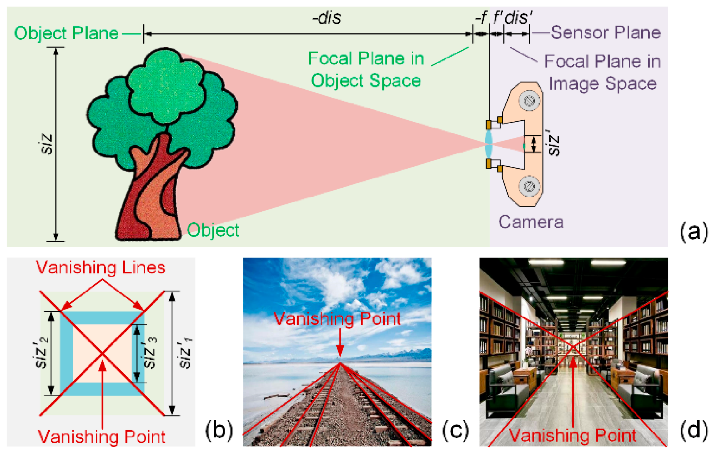
Currently, 2D images are usually captured by 2D cameras. Most 2D cameras can be simplified as lens-based imaging systems, as shown in Figure 1a. When dis is the distance between the object and the focal plane in the object space, f is the focal length in the object space, and siz is the size of the object, then the size of the object in the captured 2D image siz′ can be obtained from Newton’s image formula (Equation (1)):

$${siz}^{\prime }=\frac{f}{dis}\times siz$$

(1)

An object located at an infinite distance from the lens appears to be a point in a 2D image. This point is called the vanishing point. In a 2D image, as the distance to the vanishing point changes, objects with a same size appear to be distributed along divergent lines originating at the vanishing point, as shown in Figure 1b. These divergent lines are called vanishing lines.

There are two types of 2D images that contain a vanishing point and vanishing lines. The first type is a 2D image with a large shooting distance. These images are often captured outdoors, and typically present the sky, land areas, and water bodies. These type of images are referred to as distant view images, which primarily capture scenes on the horizontal plane. The second type is a 2D image with a moderate shooting distance, and such images contain an obvious perspective effect. The scenes on both the horizontal and vertical planes are presented, and such images are referred to as perspective images. The vanishing point of a distant view image is always located on the borderline between the sky and other physical elements (Figure 1c), while that of a perspective image is located near the central area of the image (Figure 1d).

The CGDMs of these two types of 2D images are calculated according to different depth gradient models in the proposed method. Therefore, the image type should be firstly identified. Identification of a distant view image uses the color feature. The 2D image is transformed from the RGB color space to the hue-saturation-intensity (HSI) color space [35]. Pixels representing the sky, land areas, and water bodies, have typical pixel values in the range [36]:

$$Pixel Value\in \left\{\begin{array}{c}\left(\left(80<I<255\right)\& \&\left(100<H<180\right)\right)\\ \left|\right| \left(\left(80<S<255\right)\& \&\left(20<H<100\right)\right)\end{array}\right\}$$

(2)

where H, S, and I are the hue, saturation, and intensity, respectively. In addition, p is the proportion of the pixels whose values are in the above range (Equation (2)). When p > 0.5, the 2D image is classified as a distant view type.

Because the vanishing point of a distant view image is always located on the borderline between the sky and other physical elements, the CGDM is calculated using a cumulative horizontal edge histogram [37]. In this model, the sky is assumed to be infinitely far from the observer. The distances to other physical elements are linearly far-to-near, from the top edge of the image to its bottom edge. The borderline is therefore distinguished first, and subsequently the CGDM depth (x, y) can be expressed as:

$$depth\left(x,y\right) =\frac{2^{BD}-1}{N-y_{bo}}\left(y-y_{bo}\right)$$

(3)

where BD is the bit depth of the CGDM, N is the pixel number of the CGDM in the vertical direction, and y_bo is the vertical coordinate value of the borderline. A larger pixel value indicates that the point is nearer to the observer. The pixel value for the sky is assigned as zero. As the distant view image appears far-to-near, extraction of the vanishing point and vanishing lines is unnecessary in the cumulative horizontal edge histogram.

2.2. Perspective View Images

If p ≤ 0.5, it is necessary to determine if the 2D image is a perspective type. This is determined by edges extracted from the original image. Edges in the 2D image are extracted using Canny algorithm [38]. The Hough transform [39] is used to detect straight lines from the edges. If and only if straight lines intersect at one point, the intersection is regarded as a vanishing point. The existence of a vanishing point is key to determining whether the 2D image belongs to the perspective type.

For the perspective image, the vanishing point is regarded as the farthest point. Since a typical perspective scene will contain image data in both the horizontal and vertical planes, the CGDMs for content on the two planes are calculated separately. Vanishing lines are used to distinguish the horizontal and vertical planes [40]. The CGDMs can be calculated by:

$$depth\_h\left(x,y\right) =\frac{2^{BD}-1}{N-y_{vp}}\left(y-y_{vp}\right)$$

(4)

$$depth\_v\left(x,y\right) =\frac{2^{BD}-1}{M-x_{vp}}\left(x-x_{vp}\right)$$

(5)

where depth_h and depth_v are the depth gradients on the horizontal and vertical planes, respectively. Additionally, (x_vp, y_vp) is the coordinate value of the vanishing point, and M and N are the number of pixels in the CGDM in the horizontal and vertical directions, respectively. For content on the horizontal plane, the depth gradient is assigned 0 to 255 along the columns, from the vanishing point to the edge of the CGDM. For content on the vertical plane, the depth gradient is assigned 0 to 255 along the rows.

Sometimes the position of the vanishing point is not located in the central area of the image. The depth gradient of the holographic reconstruction might be different from the reality in this case. To avoid depth error in the holographic reconstruction, some adjustments are conducted when calculating the CGDM. Firstly, the image should be expanded to twice the original size by zero-padding. Secondly, the vanishing point of the image is searched. The padded image should be cropped with the vanishing point as the center and the maximum length from the vanishing point to the edge of image as the side length. Thirdly, the CGDM of the cropped image is calculated. The depth map of the original image is obtained by cutting the CGDM of the cropped image.

2.3. Close-Up Images

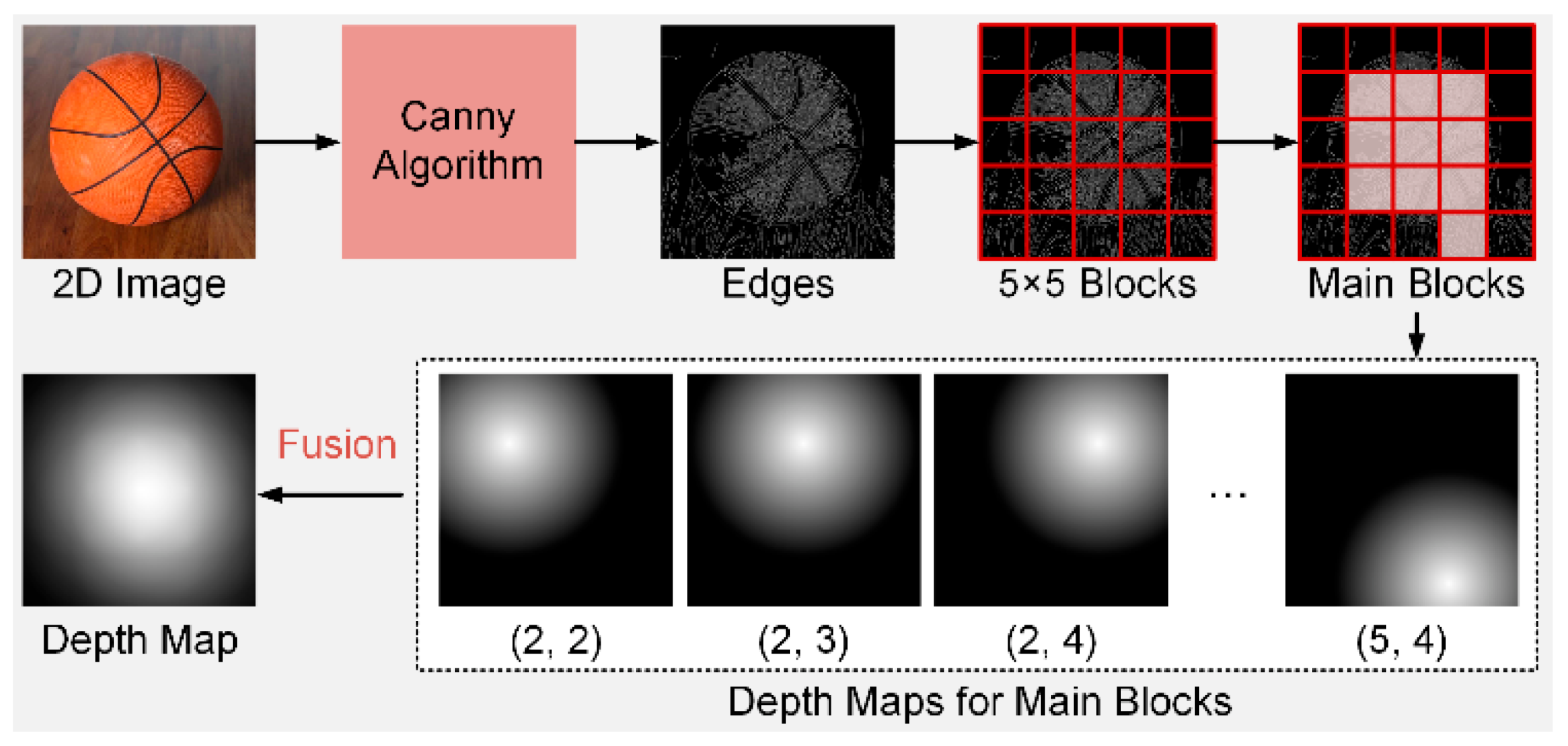
If no convergence point is detected in the image, or multiple convergence points are detected, the image will be classified as a close-up image, rather than a perspective view image. For a close-up image, the CGDM can be found using occlusion [41]. Regions that contain fewer edges generally represent that they are farther away. The spatial relationship of a series of objects with multiple depths can be easily determined by counting the amount of edges. The local edge histogram [40] is employed to calculate the CGDM. As shown in Figure 2, the edges of the 2D image are first extracted by Canny algorithm. Then, the image of the edges is divided into 5 × 5 blocks. The number of edges N_ij in each block is counted. Blocks where N_ij is larger than the average (N_av) are defined as the main blocks. The total number of main blocks is M, while the number of edges in each main block is denoted by N₁′, N₂′, …, N_M′. From a series of simulations, the reliable CGDM for each main block is proved to be a circle with a depth gradient. The center of the circle locates at the center of the corresponding block. The pixel values of the center and the circumference are assigned as 255 and 0, respectively. Meanwhile, the pixel value decreases evenly from the center to the circumference. The radius of the circle is obtained by traversal comparisons, and an optimized radius is the half the length (or width) of the image. The CGDM for the entire close-up image is obtained by fusing together the depth maps of the main blocks. If D_i is the CGDM of the lth main block, the fused CGDM D_f can be expressed as:

$$D_f={\displaystyle \sum _{i=1}^M\left(D_i\times \frac{{N_i}^{\prime }}{{\displaystyle \sum _{i=1}^M{N_i}^{\prime }}}\right)}$$

(6)

3. Calculation and Reconstructions of CGHs

3.1. Calculation of CGHs

A layer-based holographic algorithm [42] is employed to calculate the CGHs. Because an 8-bit CGDM is employed, the 3D model obtained by 2D-to-3D rendering is sliced into 256 parallel layers. A random phase r (x, y) is superposed on each layer to simulate the diffusive effect of the object surface. The complex amplitude distribution on the holographic plane E_com (x, y) is calculated as follows:

$$E_{com}\left(x,y\right) ={\displaystyle \sum _{l=0}^{255}\left\{{\mathrm{FT}}^{-1}\left\{\mathrm{FT}\left\{U_l\left(x,y\right)\exp \left[ir\left(x,y\right)\right]\right\}\left.\exp \left[i2\pi z_l\sqrt{1-{\left(\lambda u\right)}^2-{\left(\lambda v\right)}^2}/\lambda \right]\right\}\right.\right\}}$$

(7)

$$u= \left(\cos \alpha \right)/\lambda ,v= \left(\cos \beta \right)/\lambda$$

(8)

where FT represents the Fourier transform, U_l (x, y) is the amplitude of the lth layer, z_l is the distance between the lth layer and the holographic plane, λ is the wavelength, u and v are the spatial frequencies, and α and β are the angles between the incident wave and the x- and y-directions, respectively. As this study uses a phase-only spatial light modulator (SLM), the phase-only distribution E_p (x, y) should be extracted from E_com (x, y) (Equation (7)).

3.2. Reconstruction of CGHs

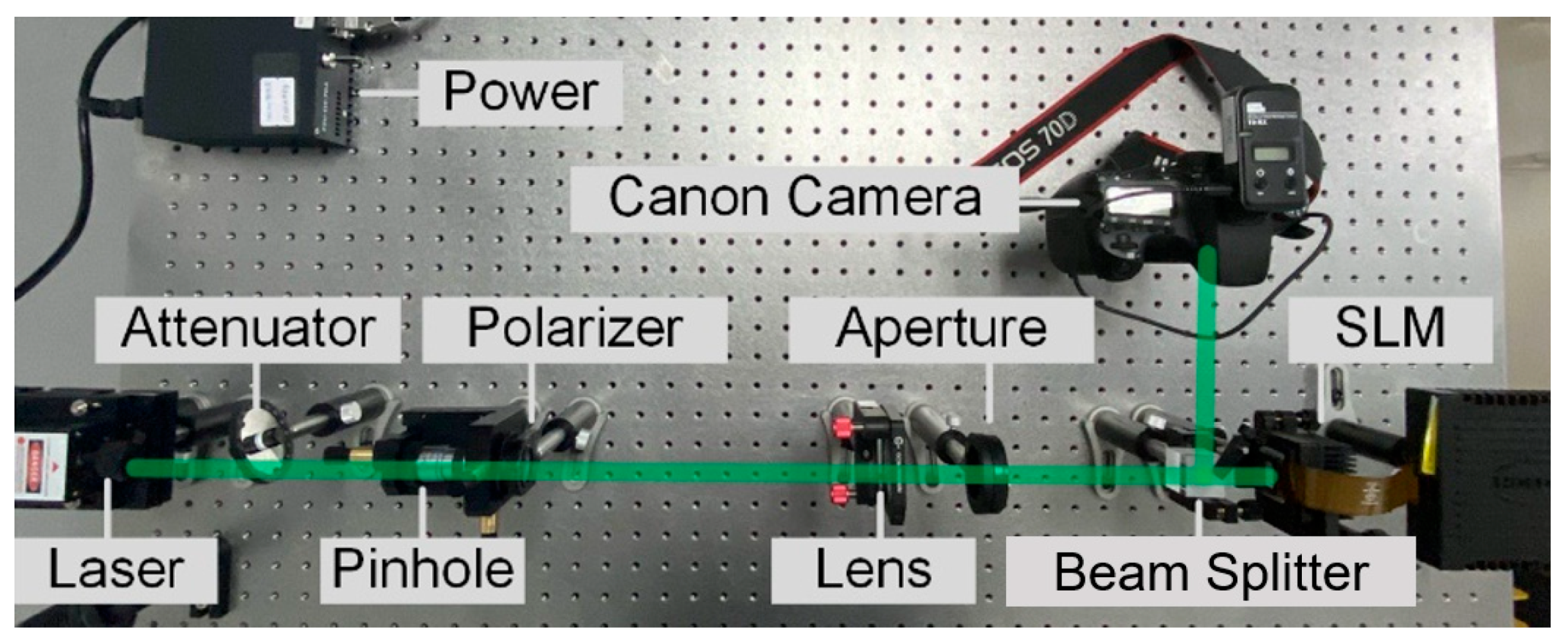
To verify the effectiveness of the 2D-to-3D rendering approach in practical applications, we built a phase-only holographic display system, as shown in Figure 3. The illumination laser beam was filtered by a pinhole and collimated by a lens. The CGH of was uploaded on a phase-only SLM. The SLM employed in the system was a Holoeye Gaea-2 VIS. After being modulated by the CGH on the SLM, the reconstructed wavefront was captured by a Canon 60D digital camera.

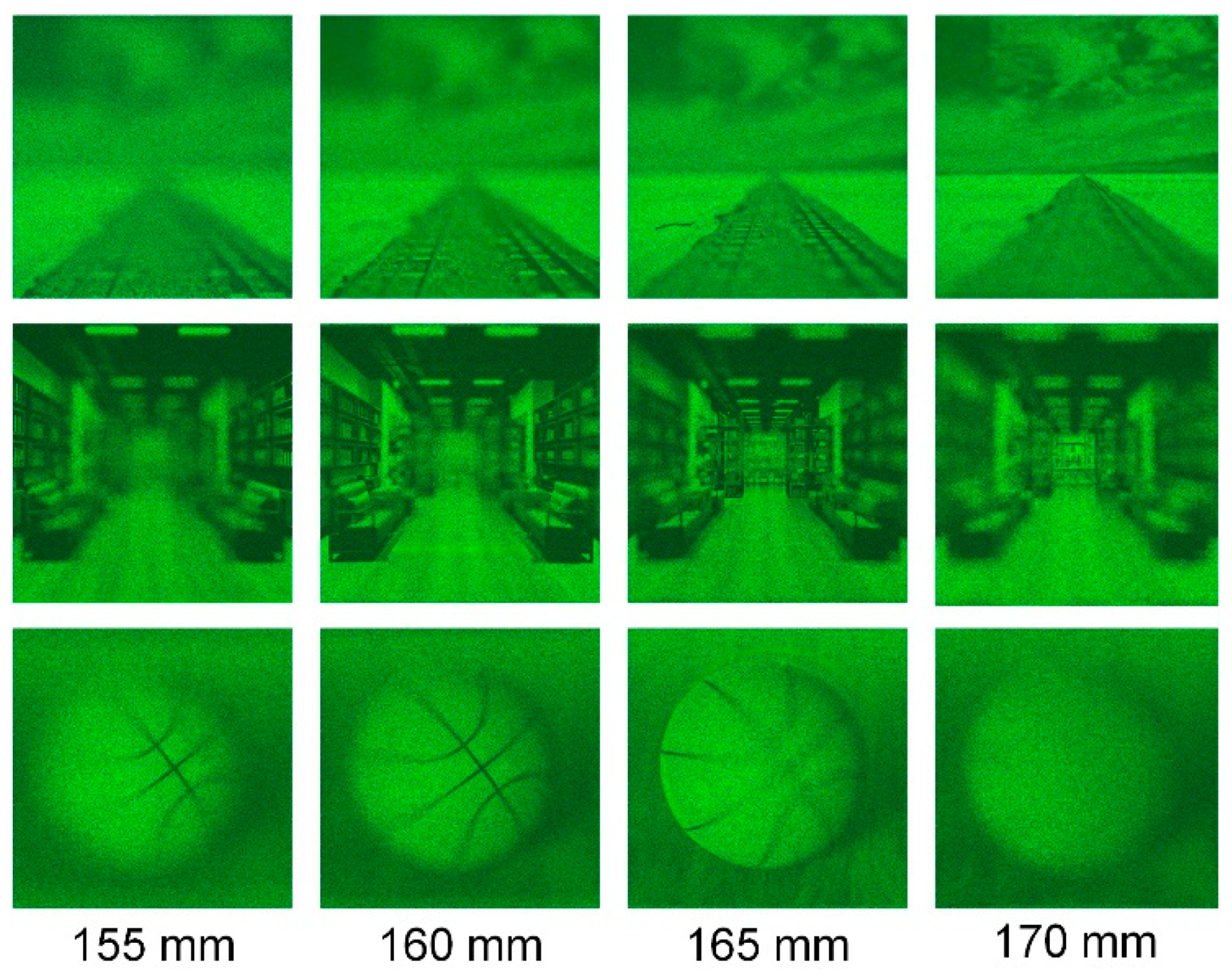
In the experimental system, the illumination wavelength, pixel pitch, and resolution of the CGH are 532 nm, 3.74 μm and 2000 × 2000, respectively. During the experiments, the camera is placed at shooting distances of 155, 160, 165, and 170 mm, respectively. The captured results are shown in Figure 4. When the shooting distance is 155 mm, the part of the reconstruction that is nearest to the camera is clear, while the distant part is blurred. As the shooting distance varies, the focus position of the reconstruction also changes. Hence, a 3D effect can be obtained using CGDMs in this 2D-to-3D rendering approach.

4. Discussion

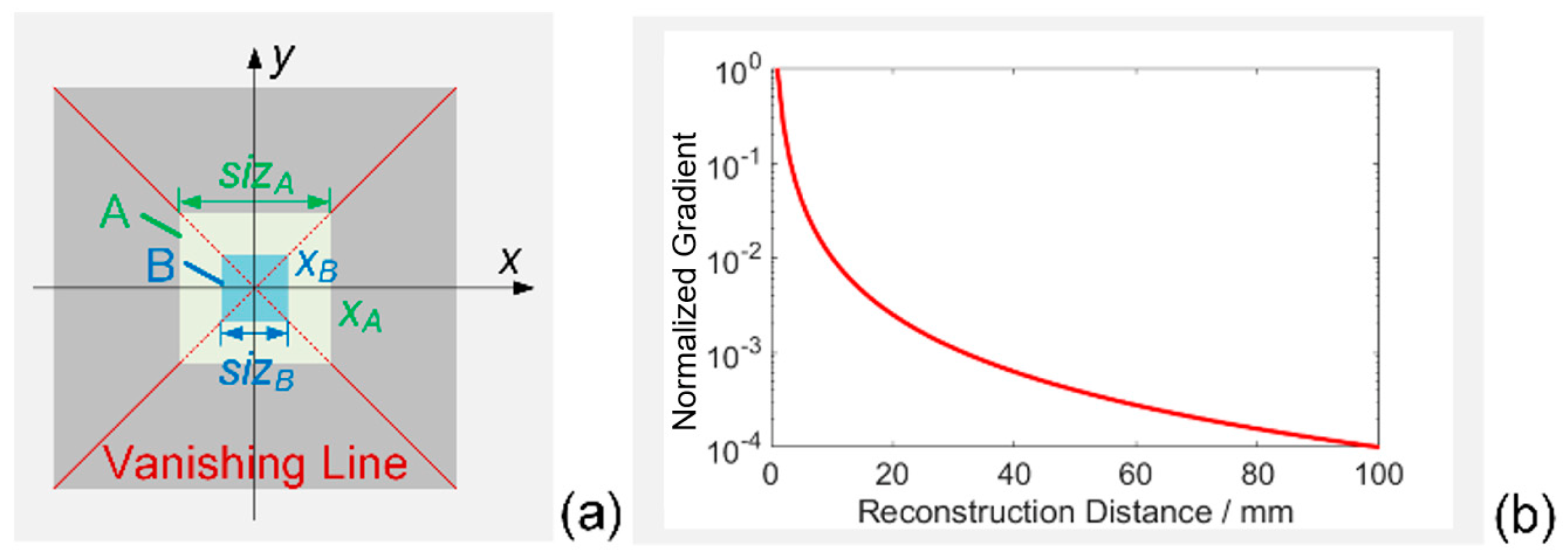
In Figure 5a, objects A and B are the same size, but are placed at different shooting distances. Thus, their sizes in the captured 2D image are different, siz_A and siz_B, respectively. For simplification, only the image sizes in the x-direction x_A and x_B are discussed. The pixel value of the CGDM changes linearly along the vanishing line. Thus, the CGDM values for these two objects, depth_A and depth_B, are proportional to their sizes. From Equation (1), the relationship between the real shooting distance and the pixel value of the CGDM can be expressed as:

$$\left(dept{h}_A-dept{h}_B\right) \propto \left(x_A-x_B\right) =-fx\frac{di{s}_A-di{s}_B}{di{s}_{A}di{s}_B}$$

(9)

When Δdepth is infinitely small, Equation (9) can be rewritten as:

$$k=\frac{\mathsf{\Delta }depth}{\mathsf{\Delta }dis}\propto \frac{1}{di{s}^2}$$

(10)

As the shooting distance increases, each increment in the CGDM gray scale represents a larger change in depth, as shown in Figure 5b. The human eye’s perception of depth information wanes as the observation distance increases. Thus, human factor engineering is fully considered during the design of the CGDM.

In this study, the average processing time for the image classification, CGDM calculation, and CGH generation are 9.67, 87.33, and 1201.67 ms, respectively. The total calculation time is 1298.67 ms, which limits the application of the proposed approach in dynamic 3D display. Considering that both the calculation of CGDMs and the generation of CGHs can be realized by deep learning [43], further optimization of the calculation time would be practical. Combining the proposed method with deep learning network is the future direction of the work.

5. Conclusions

Adoption of holographic 3D displays is inhibited by the dearth of rich 3D content. To address this issue, we successfully demonstrate a layer-based holographic algorithm by applying 2D images to a 2D-to-3D rendering approach. In this study, 2D images are first classified into three categories: the distant view, perspective, and close-up types. A cumulative horizontal edge histogram, vanishing line method, and local edge histogram are employed to calculate the CGDMs. The layer-based holographic algorithm is then employed to calculate the CGHs for 3D models obtained by the 2D-to-3D approach. Identical 3D variations are obtained in the reconstructions of 2D images. The average processing time is approximately 1200 ms. Further improvement of the CGH calculation time would assist application of the proposed approach in dynamic holographic displays.

References

- Kim, M.K. Full color natural light holographic camera. Opt. Express 2013, 21, 9636–9642. [Google Scholar] [CrossRef] [PubMed]
- Lee, K.R.; Park, Y.K. Exploiting the speckle-correlation scattering matrix for a compact reference-free holographic image sensor. Nat. Commun. 2016, 7, 13359. [Google Scholar] [CrossRef] [PubMed] [Green Version]
- Antipa, N.; Kuo, G.; Heckel, R.; Mildenhall, B.; Bostan, E.; Ng, R.; Waller, L. DiffuserCam: Lensless single-exposure 3D imaging. Optica 2018, 5, 1–9. [Google Scholar] [CrossRef]
- Bradley, M.; Sabatier, J.M. Applications of Fresnel-Kirchhoff diffraction theory in the analysis of human-motion Doppler sonar grams. J. Acoust. Soc. Am. 2010, 128, EL248. [Google Scholar] [CrossRef] [PubMed]
- Zhang, W.; Hoorfar, A. Three-dimensional real-time through-the-wall radar imaging with diffraction tomographic algorithm. IEEE Trans. Geosci. Remote Sens. 2013, 51, 4155–4163. [Google Scholar] [CrossRef]
- Lee, M.K. Wide area quantitative phase microscopy by spatial phase scanning digital holography. Opt. Lett. 2020, 45, 784–786. [Google Scholar]
- Wu, L.; Zhang, Z. Domain multiplexed computer-generated holography by embedded wavevector filtering algorithm. PhotoniX 2021, 2, 1. [Google Scholar] [CrossRef]
- Wang, Z.; Zhang, X.; Lv, G.; Feng, Q.; Ming, H.; Wang, A. Hybrid holographic Maxwellian near-eye display based on spherical wave and plane wave reconstruction for augmented reality display. Opt. Express 2021, 29, 4927–4935. [Google Scholar] [CrossRef]
- Wang, Z.; Zhang, X.; Tu, K.; Lv, G.; Feng, Q.; Wang, A.; Ming, H. Lensless full-color holographic Maxwellian near-eye display with a horizontal eyebox expansion. Opt. Lett. 2021, 46, 4112–4115. [Google Scholar] [CrossRef]
- Wang, D.; Zheng, Y.-W.; Li, N.-N.; Wang, Q.-H. Holographic display system to suppress speckle noise based on beam shaping. Photonics 2021, 8, 204. [Google Scholar] [CrossRef]
- He, Z.; Sui, X.; Zhang, H.; Jin, G.; Cao, L. Frequency-based optimized random phase for computer-generated holographic display. Appl. Opt. 2021, 60, A145–A154. [Google Scholar] [CrossRef]
- Wang, D.; Liu, C.; Shen, C.; Wang, Q.-H. Holographic capture and projection system of real object based on tunable zoom lens. PhotoniX 2020, 1, 6. [Google Scholar] [CrossRef] [Green Version]
- Zhao, Y.; Cao, L.; Zhang, H.; Tan, W.; Wu, S.; Wang, Z.; Yang, Q.; Jin, G. Time-division multiplexing holographic display using angular-spectrum layer-oriented method. Chin. Opt. Lett. 2016, 14, 010005. [Google Scholar] [CrossRef]
- Keil, J.; Edler, D.; Dickmann, F. Preparing the Hololens for user studies: An augmented reality interface for the spatial adjustment of holographic objects in 3D indoor environments. J. Cartogr. Geogr. Inf. 2019, 69, 205–215. [Google Scholar] [CrossRef] [Green Version]
- Wyss, C.; Bührer, W.; Furrer, F.; Degonda, A.; Hiss, J.A. Innovative teacher education with the augmented reality device Microsoft Hololens—results of an exploratory study and pedagogical considerations. Multimodal Technol. Interact. 2021, 5, 45. [Google Scholar] [CrossRef]
- Keil, J.; Korte, A.; Ratmer, A.; Edler, D.; Dickmann, F. Augmented reality (AR) and spatial cognition: Effects of holographic grids on distance estimation and location memory in a 3D indoor scenario. J. Photogramm. Remote Sens. Geoinf. Sci. 2020, 88, 165–172. [Google Scholar] [CrossRef]
- Moro, C.; Phelps, C.; Redmond, P.; Stromberga, Z. HoloLens and mobile augmented reality in medical and health science education: A randomised controlled trial. Br. J. Educ. Technol. 2020, 52, 680–694. [Google Scholar] [CrossRef]
- Mishina, T.; Okui, M.; Okano, F. Calculation of holograms from elemental images captured by integral photography. Appl. Opt. 2006, 45, 4026–4036. [Google Scholar] [CrossRef]
- Yanagihara, H.; Kakue, T.; Yamamoto, Y.; Shimobaba, T.; Ito, T. Real-time three-dimensional video reconstruction of real scenes with deep depth using electro-holographic display system. Opt. Express 2019, 27, 15662–15678. [Google Scholar] [CrossRef]
- Yamaguchi, M. Light-field and holographic three-dimensional displays. J. Opt. Soc. Am. A 2016, 33, 2348–2364. [Google Scholar] [CrossRef]
- Igarashi, S.; Nakamura, T.; Matsushima, K.; Yamaguchi, M. Efficient tiled calculation of over-10-gigapixel holograms using ray-wavefront conversion. Opt. Express 2018, 26, 10773–10786. [Google Scholar] [CrossRef]
- Tsai, S.-F.; Cheng, C.-C.; Li, C.-T.; Chen, L.-G. A real-time 1080p 2D-to-3D video conversion system. IEEE Trans. Consum. Electron. 2011, 57, 915–922. [Google Scholar] [CrossRef]
- Cheng, C.-C.; Li, C.-T.; Chen, L.-G. A novel 2D-to-3D conversion system using edge information. IEEE Trans. Consum. Electron. 2010, 56, 1739–1745. [Google Scholar] [CrossRef]
- Lai, Y.-K.; Lai, Y.-F.; Chen, Y.-C. An effective hybrid depth-generation algorithm for 2D-to-3D conversion in 3D displays. J. Disp. Technol. 2013, 9, 154–161. [Google Scholar] [CrossRef]
- Zhang, Z.; Yin, S.; Liu, L.; Wei, S. A real-time time-consistent 2D-to-3D video conversion system using color histogram. IEEE Trans. Consum. Electron. 2015, 61, 524–530. [Google Scholar] [CrossRef]
- Gil, J.; Kim, M. Motion depth generation using MHI for 2D-to-3D video conversion. Electron. Lett. 2017, 53, 1520–1522. [Google Scholar] [CrossRef]
- Tsai, T.-H.; Fan, C.-S.; Huang, C.-C. Semi-automatic depth map extraction method for stereo video conversion. In Proceedings of the 6th International Conference on Genetic and Evolutionary Computing (ICGEC 2012), Kitakyushu, Japan, 25–28 August 2012; pp. 340–343. [Google Scholar]
- Boleček, L.; Říčný, V. The estimation of a depth map using spatial continuity and edges. In Proceedings of the 36th International Conference on Telecommunications and Signal Processing (TSP 2013), Rome, Italy, 2–4 July 2013; pp. 890–894. [Google Scholar]
- Yang, Y.; Hu, X.; Wu, N.; Wang, P.; Xu, D.; Rong, S. A depth map generation algorithm based on saliency detection for 2D to 3D conversion. 3D Res. 2017, 8, 29. [Google Scholar] [CrossRef]
- Brox, T.; Bruhn, A.; Papenberg, N.; Weickert, J. High accuracy optical flow estimation based on a theory for warping. In Proceedings of the 8th European Conference on Computer Vision (ECCV 2004), Prague, Czech Republic, 11–14 May 2004; pp. 25–36. [Google Scholar]
- Laina, I.; Rupprecht, C.; Belagiannis, V.; Tombari, F.; Navab, N. Deeper depth prediction with fully convolutional residual networks. In Proceedings of the 4th International Conference on 3D Vision (3DV 2016), Stanford, CA, USA, 25–28 October 2016; pp. 239–248. [Google Scholar]
- Sun, D.; Yang, X.; Liu, M.-Y.; Kautz, J. PWC-Net: CNNs for optical flow using pyramid, warping, and cost volume. In Proceedings of the 2018 Conference on Computer Vision and Pattern Recognition (CVPR 2018), Salt Lake City, UT, USA, 18–23 June 2018; pp. 8934–8943. [Google Scholar]
- Song, M.; Kim, W. Depth estimation from a single image using guided deep network. IEEE Access 2019, 7, 142595–142606. [Google Scholar] [CrossRef]
- Ranftl, R.; Lasinger, K.; Hafner, D.; Schindler, K.; Koltun, V. Towards robust monocular depth estimation: Mixing datasets for zero-shot cross-dataset transfer. IEEE Trans. Pattern Anal. Mach. Intell. 2020. early access. [Google Scholar] [CrossRef]
- Perez, F.; Koch, C. Toward color image segmentation in analog VLSI: Algorithm and hardware. Int. J. Comput. Vis. 1994, 12, 17–42. [Google Scholar] [CrossRef] [Green Version]
- Huang, Y.-S.; Cheng, F.-H.; Liang, Y.-H. Creating depth map from 2D scene classification. In Proceedings of the 2008 3rd International Conference on Innovative Computing Information and Control, Dalian, China, 18–20 June 2008; p. 69. [Google Scholar]
- Cheng, C.-C.; Li, C.-T.; Chen, L.-G. An ultra-low-cost 2-D/3-D video-conversion system. SID Symp. Dig. Tech. Pap. 2010, 41, 766–769. [Google Scholar] [CrossRef]
- Canny, J. A computational approach to edge detection. IEEE Trans. Pattern Anal. Mach. Intell. 1986, 8, 679–698. [Google Scholar] [CrossRef]
- Ballard, D.H. Generalizing the Hough transform to detect arbitrary shapes. Pattern Recognit. 1981, 13, 111–122. [Google Scholar] [CrossRef] [Green Version]
- Battiato, S.; Curti, S.; La Cascia, M.; Tortora, M.; Scordato, E. Depth map generation by image classification. Proc. SPIE 2004, 5302, 95–104. [Google Scholar]
- Yin, S.; Dong, H.; Jiang, G.; Liu, L.; Wei, S. A novel 2D-to-3D video conversion method using time-coherent depth maps. Sensors 2015, 15, 15246–15264. [Google Scholar] [CrossRef] [Green Version]
- Zhao, Y.; Cao, L.; Zhang, H.; Kong, D.; Jin, G. Accurate calculation of computer-generated holograms using angular-spectrum layer-oriented method. Opt. Express 2015, 23, 25440–25449. [Google Scholar] [CrossRef]
- Wu, J.; Liu, K.; Sui, X.; Cao, L. High-speed computer-generated holography using an autoencoder-based deep neural network. Opt. Lett. 2021, 46, 2908–2911. [Google Scholar] [CrossRef]
Figure 1.
Images captured by lens-based imaging systems. (a) Relationship between size of an image and shooting distance in a lens-based imaging system. (b) Same size objects distributed along the vanishing lines. (c) Vanishing point in distant view image. (d) Vanishing point in perspective image.
Figure 2.
Calculation of the CGDM for a close-up image.
Figure 3.
The phase-only holographic display system.
Figure 4.
Reconstructions of 3D scenes by 2D-to-3D rendering method at depths of 155 mm, 160 mm, 165 mm and 170 mm, respectively.
Figure 5.
The relationship between shooting distance and gray scale in CGDM. (a) Variation of CGDM with shooting distance (same size objects). (b) Normalized gradient of CGDM variation with shooting distance.
Publisher’s Note: MDPI stays neutral with regard to jurisdictional claims in published maps and institutional affiliations. |
© 2021 by the authors. Licensee MDPI, Basel, Switzerland. This article is an open access article distributed under the terms and conditions of the Creative Commons Attribution (CC BY) license (https://creativecommons.org/licenses/by/4.0/).
Share and Cite
MDPI and ACS Style
He, Z.; Sui, X.; Cao, L. Holographic 3D Display Using Depth Maps Generated by 2D-to-3D Rendering Approach. Appl. Sci. 2021, 11, 9889. https://0-doi-org.brum.beds.ac.uk/10.3390/app11219889
AMA Style
He Z, Sui X, Cao L. Holographic 3D Display Using Depth Maps Generated by 2D-to-3D Rendering Approach. Applied Sciences. 2021; 11(21):9889. https://0-doi-org.brum.beds.ac.uk/10.3390/app11219889
Chicago/Turabian StyleHe, Zehao, Xiaomeng Sui, and Liangcai Cao. 2021. "Holographic 3D Display Using Depth Maps Generated by 2D-to-3D Rendering Approach" Applied Sciences 11, no. 21: 9889. https://0-doi-org.brum.beds.ac.uk/10.3390/app11219889
Note that from the first issue of 2016, this journal uses article numbers instead of page numbers. See further details here.