
Revising of the Near Ground Helicopter Hover: The Effect of Ground Boundary Layer Development


1
Department of Fluid Mechanics, School of Mechanical Engineering, National Technical University of Athens (NTUA), Ir. Politechniou 9, 15780 Zografou, Greece
2
Department of Naval and Marine Hydrodynamics, School of Naval Architecture and Marine Engineering, National Technical University of Athens (NTUA), Ir. Politechniou 9, 15780 Zografou, Greece
*
Author to whom correspondence should be addressed.
Appl. Sci. 2021, 11(21), 9935; https://0-doi-org.brum.beds.ac.uk/10.3390/app11219935
Submission received: 30 September 2021
/
Revised: 15 October 2021
/
Accepted: 20 October 2021
/
Published: 24 October 2021
(This article belongs to the Special Issue Aerodynamic Aeroelasticity and Aeroacoustics of Rotorcraft)
Abstract
:The interaction of a helicopter rotor with the ground in hover flight is addressed numerically using a hybrid Eulerian–Lagrangian CFD model. When a helicopter takes off or lands, its wake interferes with the ground. This interaction, depending on the height-to-rotor diameter ratio, causes the altering of the rotor loading and performance as compared to the unconstrained case and gives rise to the development of a complex outwash flow field in the surrounding of the helicopter. The present study aims to characterize the interactional phenomena occurring in the early stages of the rotor wake development and in particular the interference of the starting vortex with the ground boundary layer and the effect of this interaction in the motion of the vortex in the rotor outwash flow. The hybrid CFD method employed combines a standard URANS compressible finite volume solver, the use of which is restricted to confined grids around solid bodies, and a Lagrangian approximation of the entire flow field in which conservation equations are solved in their material form, disctretized using particle representation of the flow quantities. The two methods are strongly coupled to each other through an appropriate iterative scheme. The main advantage of the proposed methodology is that it can conveniently handle complex configurations with several bodies that move independently from one another, with affordable computational cost. In this paper, thrust coefficient predictions of the hybrid model are compared to predictions of a free wake code and to experimental data indicating that consistent prediction of the rotor load requires the inclusion of the ground boundary layer in the analysis. Moreover, detailed comparisons of the rotor wake evolution predicted by the hybrid model are presented.
1. Introduction
When a helicopter executes hover flight during takeoff and landing, a complex flow field is developed in the wake of its main rotor which is affected by the blockage of the ground. The starting vortex ring of the rotor impinges on the ground and thereafter a so-called “ground vortex” is formed that moves outwards forming an outwash flow. The formation and the intensity of the ground vortex depend on several parameters such as the helicopter distance from the ground; the wind velocity and direction, if any; and the thickness of the boundary layer on the ground. The presence of the ground near the rotor has been known to alter the aerodynamics of the rotor In Ground Effect (IGE) as compared to Out of Ground Effect (OGE) and gives rise to performance benefits (reduced power consumption for a given thrust), however there are also reports of operational and handling issues [1].
The rotor wake–ground interference has been addressed in several experimental and numerical studies. Curtiss et al. [2] conducted IGE experiments in an in-door test rig. An isolated rotor was towed in a long towing shed. They measured the loads of the rotor for different values of the advance ratio within the range 0–0.1 and for different flight height–to-rotor diameter ratios within the range 0.23–0.45. They distinguished two wake flow states:
- (i)
- the re-circulation flow in which the starting vortex rolls up ahead of the rotor disk and
- (ii)
- the ground vortex flow in which the starting vortex rolls up below the rotor disk
while, through extensive flow visualization, they identified the conditions that favor the development of each of them.
In the framework of HELIFLOW project, Boer et al. [3] performed wind tunnel IGE tests during side-ward flight. The campaign took place in the large low speed facility (LLF) of the German–Dutch wind tunnel (DNW). The rotor outwash and the position of the ground vortex were measured via particle image velocimetry (PIV). Smaller scale wind tunnel IGE tests were conducted by Ganesh and Komerath in the John J. Harper Low-Speed Wind Tunnel of Georgia Institute of Technology [4] and by Nathan and Green in a low-speed, closed-return wind tunnel with a 2.7 m wide × 2.10 m high × 4 m long, octagonal working section [5]. Ganesh and Komerath measured the velocity in the wake using hot-wire anemometry, which was combined with pulsed laser sheet flow visualizations and hub-load measurements. Their objective was to characterize the unsteadiness of the wake flow in ground effect. They measured fluctuations in the rotor inflow which were found 5–10% higher than the ones corresponding to OGE. They attributed the fluctuations to the ingestion of the re-circulation flow into the rotor near wake region. Nathan and Green mimicked the relative motion of the helicopter with respect to the ground when in forward flight, by adding a moving belt on the ground level instead of the tunnel wind flow. This suggests that the presence of the ground boundary layer is essential for the correct prediction of the interactional phenomena between the rotor wake and the ground. More recently, Sugiura et al. [6] conducted IGE flight tests of the JAXA research helicopter. Velocity measurements were taken with a LIDAR system as well as ultra sonic anemometers and were combined with smoke visualizations. Sugiura et al. [7] used these measured data to validate their URANS simulations. The focus of the comparison was in forward flight cases with low advance ratios values. Cavallo et al. [8] conducted a similar study on the rotor–ground interference using URANS simulations combined with an actuator disk model of the rotor. Similar to the work in [7], the authors focused on forward flight conditions with low advance ratio values and assessed the developed flow field around the helicopter. More recently, Pasquali et al. [9] used a potential BEM solver for investigating the aerodynamics of a hovering rotor in ground effect. In the modeling of the ground, two approaches were followed by the authors. The first mimics the grounds as a infinite symmetry plane (mirroring technique), and the second treats the ground as a panel body (bounded domain method). The results in general were found to be in good agreement with measurements. However, both methods due to their inviscid character showed some limitations by predicting the increase in trust coefficient at with a deviation of ≈.
Due to its importance, the ground effect problem was also addressed in a recent GARTEUR action group (AG-22 [10]) within the broader scope of analyzing rotor–obstacle interactional phenomena. Within the group, computational tools of varying fidelity and wind tunnel experiments were employed with the aim to unravel the complex flow field and characterize the loads of a helicopter rotor flying at low altitude, in close proximity to a well shaped obstacle in addition to ground effect. A number of wind tunnel test campaigns were performed as part of this action group [11,12], while one of them, was conducted in the atmospheric flows test section of POLIMI’s wind tunnel, addressing the pure ground effect problem.
In the present paper, numerical activities addressing the rotor–ground interference problem are presented, part of which were contributed to this GARTEUR group. The work was motivated by an earlier study by the authors [13] in which the loads of a hovering helicopter main rotor in IGE were computed using a potential free wake solver [14]. The predictions were found in very good agreement with the POLIMI measured data [12] at altitudes higher than 1.5 rotor diameters. However, accuracy degraded as the distance from the ground decreased. At lower altitudes the potential solver underestimated the increase in the loads caused by ground blockage. This led to the conjecture that at low altitude flights the displacement effect induced by the development of the ground boundary layer which is absent in potential methods, becomes important and may explain the deviation of the predictions. Similar observations were also made by other participants of the same Garteur group. Schmid et al. [15] investigated the effect of the ground and of a nearby obstacle on the loading of the rotor using the UPM panel code of DLR. He compared results of UPM code to data from the same experimental database and he arrived at the same conclusion, that panel codes underestimate the increase in thrust IGE at low altitude hovering conditions by ≈.
Based on the above, in the present analysis a hybrid Computational Fluid Dynamics (CFD) model is applied that can accurately predict the formation of viscous boundary layers. The corresponding flow solver, couples a standard Eulerian finite volume solver with a Lagrangian particle approximation [16,17]. In the Eulerian part, separate grids of limited width are defined around every solid body, on which the flow equations in Eulerian description are solved. In particular for the rotor–ground interaction problem different Eulerian grids are built around the rotating blades, extending by 1.5× radius in the radial direction and by 0.5× radius around every cross section. The blades are simulated as rotating actuator lines. Although the existing CFD framework is capable of treating the blades in a fully resolved manner [16], given that the present work emphasizes on the effect of the ground boundary layer on the rotor surrounding flow, it is considered that the simple and cost effective actuator line modeling approach is sufficient for capturing rotor loads correctly without aggravating computational cost. A separate grid is defined on the ground which extends 0.5× the radius above the ground level. In order to interconnect the independent domains defined by the various grids, the entire flow is described in Lagrangian coordinates and the corresponding flow equations are solved via particle approximations in a fully coupled mode with the solutions within the Eulerian grids. The Eulerian part solves the compressible flow equations in density-velocity-pressure formulation and uses pre-conditioning at low Mach while the Lagrangian part is based on the density-dilatation-vorticity-pressure formulation. The main advantage of the hybrid model is that it can effectively deal with flow problems which involve several bodies, that move independently the one from the other while the same time resolves viscous phenomena.
2. Description of the Numerical Tools
2.1. The Eulerian Solver—MaPFlow
MaPFlow is a compressible, cell-centered finite volume CFD solver, which employs both structured and unstructured grids. The convective fluxes are discretized using Roe’s approximate Riemann solver [18] together with the Venkatakrishnan limiter [19], while the viscous fluxes are discretized using a central 2nd-order scheme. Turbulence closure includes several options; the one equation turbulence model of Spalart (SA) [20], as well as the two equation turbulence model of Menter ( SST) [21]. MaPFlow can handle both steady and unsteady flows, the latter being an important requirement for aerodynamic tools employed in helicopter analysis. Time integration is achieved in an implicit manner permitting large CFL numbers. The unsteady calculations use a 2nd order time accurate scheme combined with the dual time-stepping technique to facilitate convergence. Additionally, flows in the in-compressible regime are realized using Low Mach Preconditioning [22].
Let D denote a volume of fluid and its boundary. By integrating the governing equations over D, the following integral form is obtained:
where, , and are the convective and viscous fluxes, respectively; is the fluid density; is the flow velocity; p is the pressure; E is the total internal energy; H is the total enthalpy; denotes the viscous stress tensor; the normal velocity; and Q the source terms (if any).
Actuator Line Model
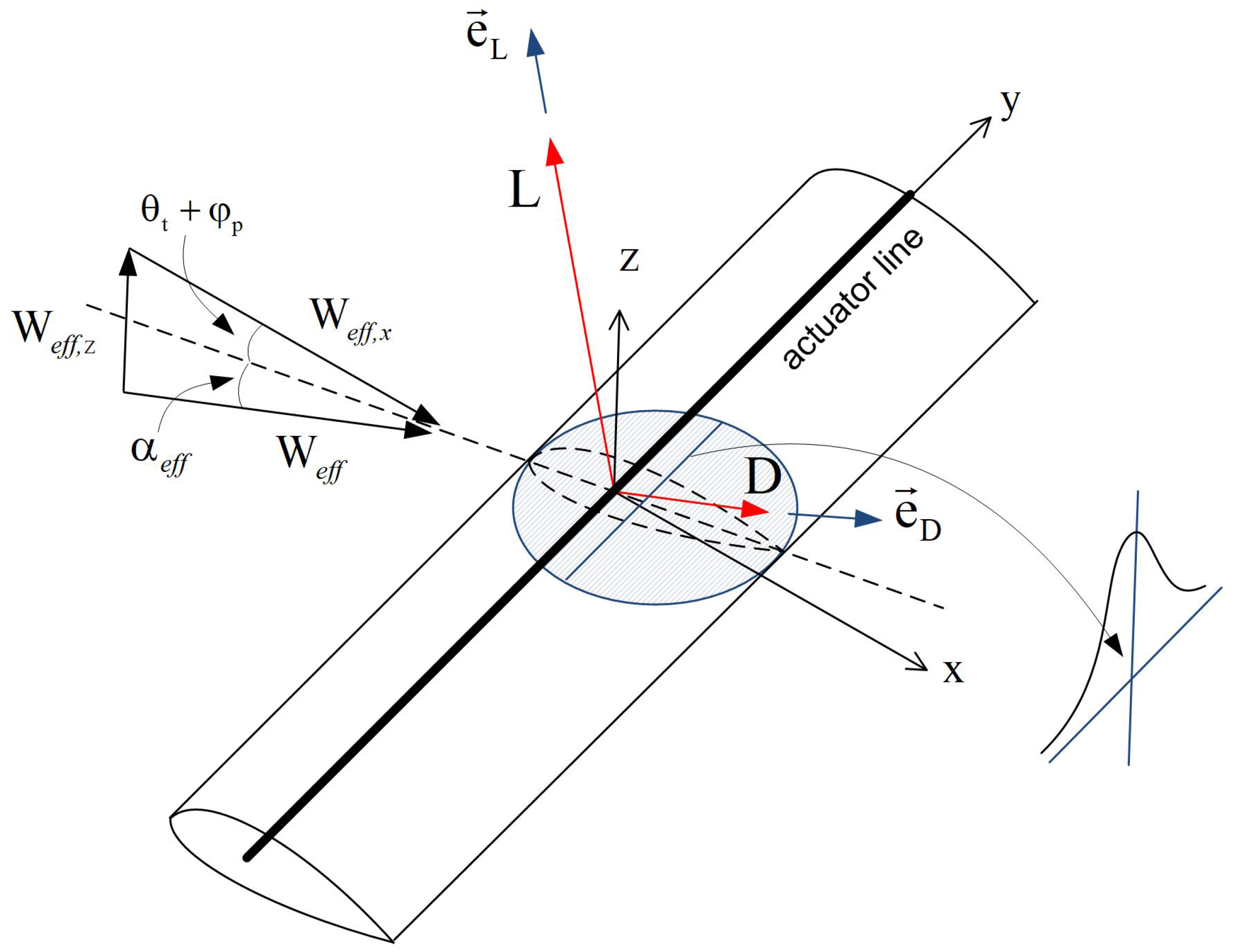
In the present work, the rotor blades are modeled as rotating actuator lines that contribute the corresponding body forces to the source term Q of the previous equation. The loading is calculated on the basis of blade element analysis along the blade span and in conjunction with tabulated polars [23]. The blade is divided in a number of elements with a span-wise extent. The centers of these elements constitute the control points of the numerical process. A lift and drag resultant body force is assigned to each actuator line control point depending on the airfoil type, twist angle, chord length, and incoming flow velocity. Lift and drag are calculated (as shown in Figure 1), by the following equations:
where is the inflow angle; is the local twist angle; is the pitch angle of the blade; is the effective angle of attack; and are the lift and drag coefficient for the specific angle of attack, respectively; is the density of the fluid; is the local two dimensional inflow velocity; c is the blade element characteristic chord; is the width of the blade element; and , are the unit vectors in the direction of lift and drag, respectively.
The reaction of this body force and the corresponding power are then imposed as source terms in the momentum and energy equations of the cells swept by the blades during their rotation. In order to avoid singularities, the body forces are distributed over a number of neighboring cells using a isotropic Gaussian distribution [24].
where is the regularization Gaussian kernel and is the distance between a cell centered grid point and the control point of a blade element.
The freestream velocity vector is directly sampled on the control points of the actuator lines [25]. The control points lie over the line of the blade bound vorticity, where blade sectional flow effects are negligible. The velocity at the control points is estimated through a distance and volume weighted interpolation to the computed velocities of the neighboring cells of CFD grid using Radial Basis Functions (RBF) [26].
Even though recommended by [26], tip correction models are not frequently applied. The reason is that as actuator lines follow the blades in their rotation, body forces are imposed in the rotating frame. Therefore, 3D wake flow is reproduced in a more realistic manner than in actuator disk method and consists of both the shed and the trailed vortices released by the blades. Prerequisite of the above is that adequately fine grid resolution is used in the vicinity of the actuator lines. With a small enough characteristic cell length of the CFD grid (grid spacing) in the range of the distributed force suggested in [27] has been found to be sufficient to resolve the tip and root vortices. In the present work, the CFD grid spacing is chosen to be in the order of . The application of tip corrections is only then required if the utilized grid is not as fine as suggested above. Coarser grid cab be considered when the priority of simulations focuses only on blade loads predictions.
2.2. Lagrangian Solver—Compressible Vortex Particles Approximation
The Lagrangian solver is configured based on particle approximations. Particles are centered at ; occupy a volume ; and carry volume integrals of density , vorticity , dilatation , and pressure :
In the above, is any of and, respectively, is any of (e.g., ). Furthermore, denotes a smooth approximation of the Dirac function [28].
In Lagrangian (material) coordinates, the flow equations for inviscid conditions take the form
where denotes evaluation at the particle position . The velocity vector is not explicitly given by the above equations. Using the Helmholtz velocity decomposition it follows that
and therefore velocity is defined by its scalar and vector potentials, and , respectively, that are both solutions of the Poisson equation with free far field conditions. Both potentials can be directly obtained through the Biot–Savart law; however the corresponding cost may be prohibitively high and therefore instead the particle mesh technique is employed.
2.3. The Particle Mesh Scheme
The Particle Mesh (PM) scheme solves Equation (10) using a fast Fourier transformation (FFT) on a uniform Cartesian grid. Even though FFT methods significantly reduce the cost of the solving Poisson equations, having a finite grid, means that boundary terms must be calculated at the outer boundaries of the grids. Because of its convolution form, the corresponding cost is high. In order to avoid such a cost penalization the James–Lackner algorithm [16] is utilized.
The first step in the Particle Mesh scheme is to transform the flow information carried by the particles into a continuous distribution. To this end, the particle quantities are projected on the PM grid using interpolation functions (see (11)). Then, the Poisson equations are solved and the velocity at the PM grid nodes is obtained through finite differences. Similarly the entire right hand side of (9) is calculated at the grid nodes. The final step is to back interpolate the information from the grid notes to particle position, using the interpolation operator (13). Finally, the Lagrangian evolution Equation (9) are integrated in time using a 4th order Runge–Kutta scheme.
where denoted the position of the grid node,
, h denotes the grid spacing and the interpolation function used. Concerning the present work a 4th order interpolation function is used which conserves the moments up to 3rd order [29].
A well-known problem in particle methods is that as the particles loose their regularity, accuracy deteriorates. A way to mitigate this inherent problem of particle methods is remeshing. Remeshing consists of repositioning the vortex blob periodically on the PM grid nodes. In the present work re-meshing takes place at each time-step.
2.4. The Hybrid Solver
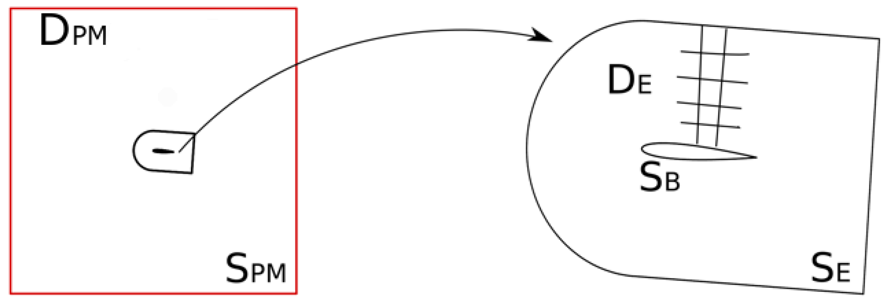
The combination of the previously described numerical methods results in a Hybrid Eulerian–Lagrangian solver (from hereon HoPFlow). A typical numerical setup for the hybrid solver can be seen in Figure 2. The computational domain is decomposed in two overlapping parts; the Eulerian one, , and the Lagrangian one . In MaPFlow CFD solver is utilized and thus wall boundary conditions on are handled exactly, which particle methods have several difficulties to efficiently implement. For the Eulerian part, boundary conditions are also needed on . They are provided by the Lagrangian solver. In this way the two solvers are coupled. Because the two domains are independent and overlapping, a correct communication between them should provide a smooth transition from one solution to the other.
Coupling is achieved by a two way communication. The Lagrangian solver provides on the boundary conditions needed for the Eulerian solver, and the Eulerian solver provides back the effect of solid boundaries on by substituting the vorticity–dilatation distributions over its defining domain .
2.4.1. Communicating the Boundary Conditions on to the Eulerian Solver
In order to solve the Eulerian equations, the correct boundary conditions on must be defined. To this end, the Lagrangian solution that is defined at the nodes of the PM grid, is interpolated at the ghost nodes of the Eulerian grid, situated outside . Next, the average over the surrounding ghost nodes indicate the flow state at the center of each ghost cell. Finally the fluxes through are determined from the Riemann invariants associated to the flow states on the two sides of .
2.4.2. Communicating the Presence of to the Lagrangian Solver
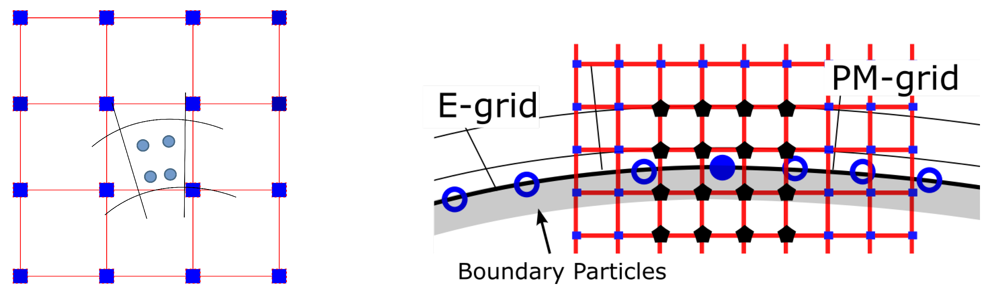
The PM grid that the Lagrangian solver is using, does not respect the solid boundaries and therefore the presence of is missing. For a Lagrangian flow description based on the formulation, flow perturbations are represented by modifications in the dilatation and vorticity fields. Assuming that the Eulerian solution in is correct if the solver is given appropriate conditions at , then the modifications in vorticity and dilatation due to are already contained in the Eulerian solution. Therefore, two steps are taken that define the coupling procedure between the Eulerian and Lagrangian parts of HoPFlow: (a) transform the Eulerian solution into compressible particles and (b) replace the Lagrangian particles contained in by those produced in step (a) (Figure 3). As the Eulerian solver is cell centered and does not use as primary quantities dilation and vorticity, step (a) includes: (i) use of Green–Gauss formula in order to obtain and at the grid nodes, (ii) interpolation of and p from cell centers at the Eulerian grid notes, and (iii) interpolation of the flow information from the Eulerian grid nodes at regular positions within every cell (in the schematic, there are four particles per cell). It is important to have good spatial density of particles, and so more than one Eulerian particles are defined per cell. Along with space particles, surfaces ones are also generated in order to obtain the correct solution near solid boundaries(Figure 3 right). The key difference is that surface intensities are multiplied by the corresponding surface in order to obtain the particle intensities. Next, space and surface particles are both projected to the PM grid in order to obtain the Lagrangian solution.
3. Description of the Test Cases
Validation is carried out against measured data from a wind tunnel test campaign, conducted at Politechnico Di Milano (Polimi) [11]. The test campaign concerns a helicopter hovering at varying distances above the ground (pure ground effect). The helicopter rotor is a four bladed one with diameter of 0.75 m. Blades are formed by NACA0012 un-tapered, untwisted airfoil sections with chord length of 0.032 m. The collective pitch was set at 10 degrees, the rotational speed at 2580 RPM and the tip Mach is equal to 0.3. The test matrix of the experiment and the simulations concern steady hover flight above the ground at different altitudes, starting from and going up to and zero wind (vertical sweep). Besides measured data-sets, predictions of the HoPFlow code are also compared to results from a previous numerical study conducted with the potential free wake solver GenUVP [13].
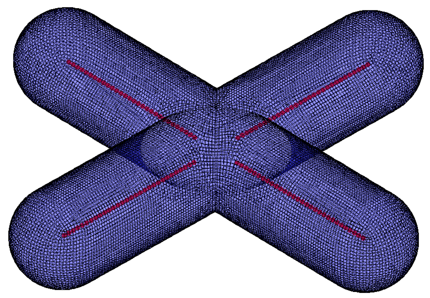
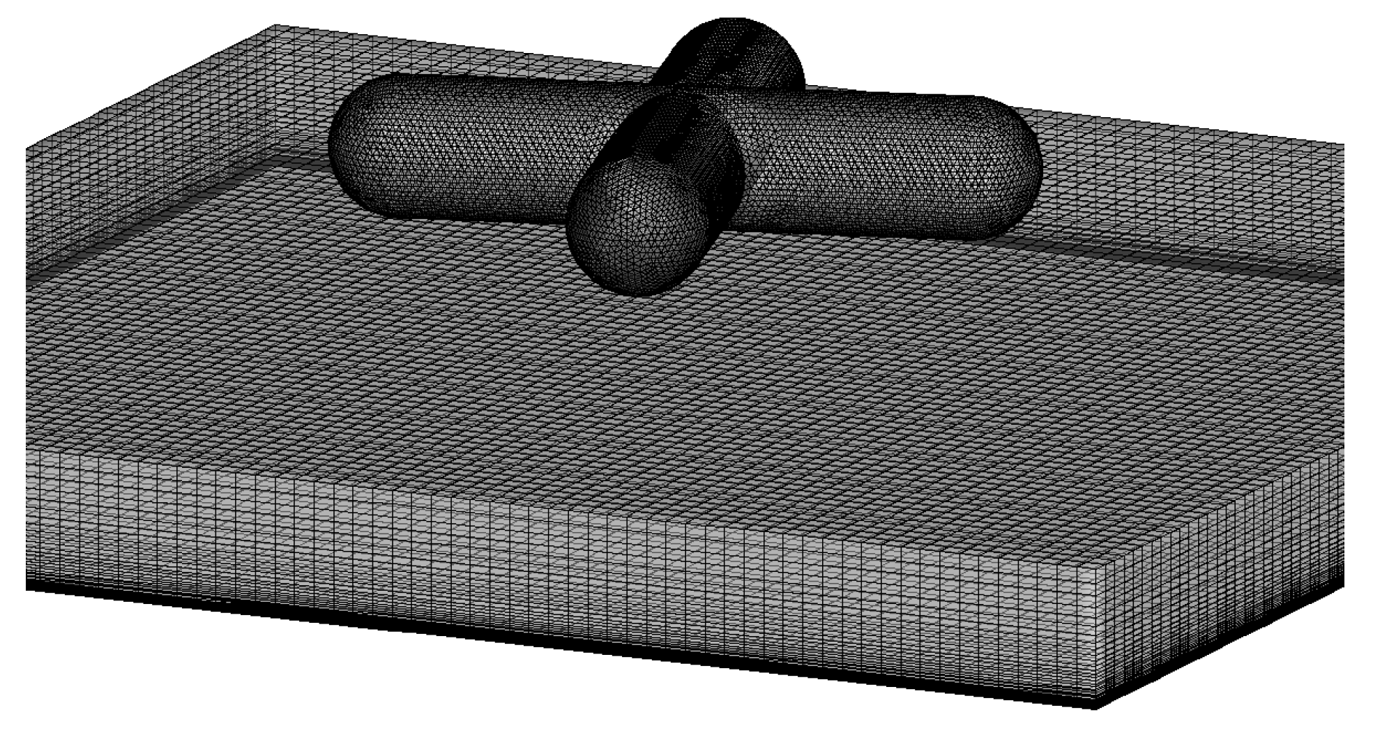
In the HoPFlow simulations, the blades are modeled as actuator lines embedded in a CFD grid of 60,000 cells (see Figure 4 and Figure 5), while the fuselage and the rotor hub are not considered. The ground is simulated as a viscous wall over which a CFD grid of 1,000,000 cells is defined with the a first cell height of m (Figure 6). The flow is considered laminar because of the moderate low velocities and Re numbers. The selection of the numerical parameters of the grid spacing has been derived from previous work [16,23]. The rest of the flow domain (between the rotor and the ground level) is filled with 2,904,000 particles. The flow velocity is determined by the PM method in which re-meshing is applied at every time step. Finally, the time step chosen corresponds to azimuth angle.
4. Validation against Measurements
4.1. Hover Flight Simulations Outside the Ground Effect (OGE)
The wind tunnel test case in which the rotor hovers at is considered as the OGE case. The measured as well as the predicted thrust values of the OGE case are shown in Table 1. Despite their many differences, both numerical methods (HoPFlow and GenUVP) predict well the thrust. The two prediction methods are based on the same airfoil polars in order to calculate the loading, which explains their agreement [30].
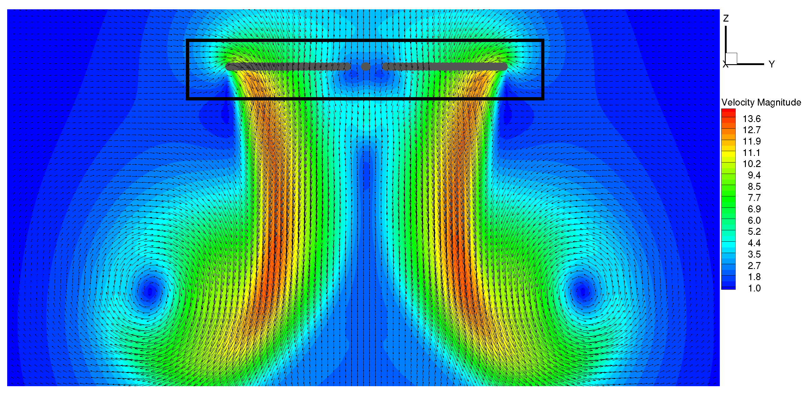
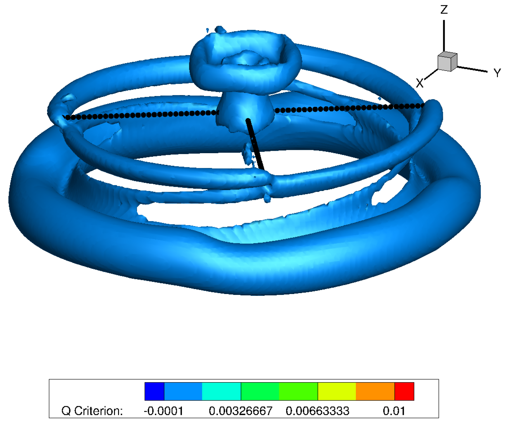
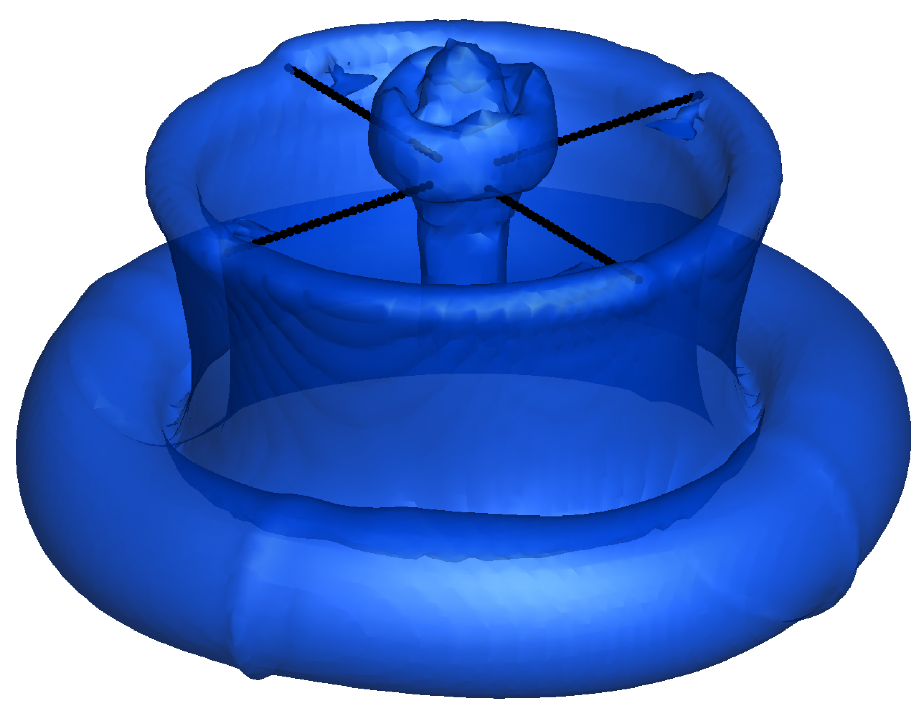
Figure 7 shows a snapshot of the OGE flow field of the hovering rotor as computed by HoPFlow after 10 rotor revolutions. Vectors and velocity contours are illustrated over a vertical plane that passes through the center of the rotor. The black box in the plot indicates the extent of the CFD grid that covers the blades. Noticeable is the continuity of the predicted flow field, in particular in the vicinity of the CFD grid boundary, which indicates that the coupling of the Eulerian method (solved within the CFD grid) with the Lagrangian method (solved over the whole computational domain) is performed in a consistent manner. Even though the actuator line model accounts for the blades as body forces that alter the momentum balance of the free flow, the model consistently reproduces the rotor wake flow in contrast to actuator disk method. This is mainly due to the fact the body forces are applied in the rotating frame of the blade and not on fixed annular elements that neglect the blades rotation as in actuator disk method. Figure 8 illustrates wake vorticity iso-surfaces at the early stages of the wake development. The figure suggests that the actuator line model captures the trailed vorticity released by the tips and roots of the blades. In Figure 9 the wake vorticity after 10 revolutions is shown. Trailed vorticity can still be recognized near the blade tips. However, in this hover case, due to the low convection velocity, wake spirals remain closely packed and strongly interact with each other producing thus the contracting shear layer of the far wake and the torus shape starting vortex ring. A similar wake pattern is obtained in the Genuvp free wake simulation (not shown in the plots).
In Figure 7, wake velocities over an axi-symmetry plain are shown. The wake vortex ring travels downstream with an average velocity of 3–4 m/s (after 10 rotor revolutions the ring has traveled 1D downwards). This ring starts to form at the very beginning of the simulation as a result of the interaction of the starting shed vortices emitted by the different blades. Moreover, the contracting jet flow that develops under the rotor disk is also visible in the flow field plot. As expected, the rotor inflow velocity varies along the blade span and obtains its maximum value within the range 70–95% of the rotor radius. In this radial range, local blade thrust also obtains its maximum value. The absence of the fuselage, hub and rotor mast, justify the hole in the flow field appearing close to the rotor center. The absence of aerodynamic loading leads to a flow field that appears to be almost stagnant in this region. The 1D distance of the starting vortex ring from the rotor plane and the convergence of the wake contracted shape indicate that after 10 revolutions the rotor loading has also converged as shown in Figure 10.
4.2. Hover Flight Simulations in IGE Flight Conditions
In helicopter hover flight in proximity to the ground, the presence of the ground has a significant (an important) effect on wake development. The starting ring vortex and the jet flow developing underneath the rotor disk, after a certain time, impinge on the ground and move outwards forming an outwash flow. The developed flow field deviates significantly from the one of the unconstrained OGE case. In simulations, ground effect can modeled either by solely imposing no-penetration (inviscid option) over the ground or by also adding zero slip (viscous option). Both options end up constraining the motion of the starting vortex, however in a different way.
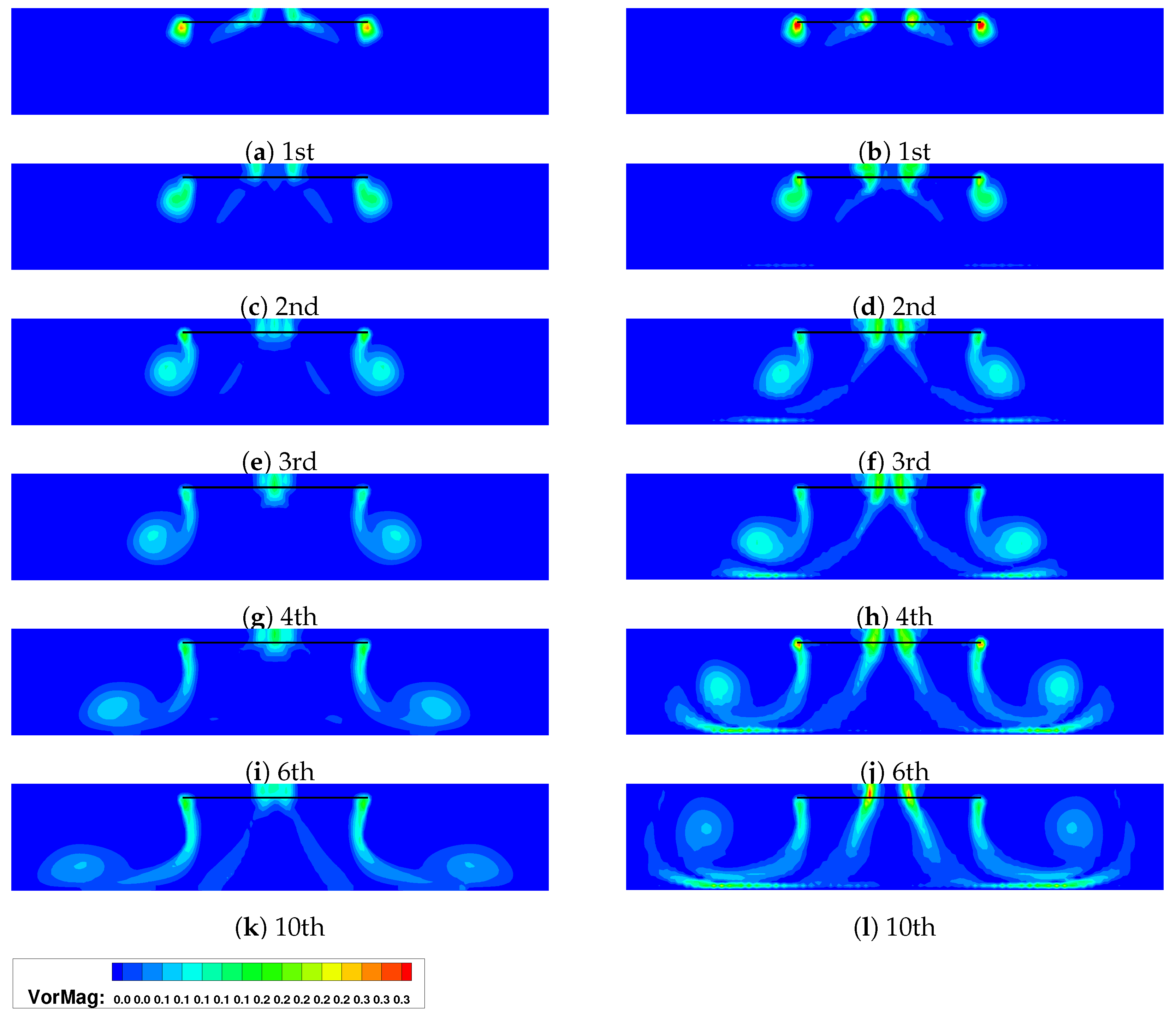
Figure 11 details in terms of vorticiy contours, the evolution of the wake that the two modeling options provide when . The inviscid option is on the left while the viscous option on the right. From top to bottom, snapshots at the end of the 1st, 2nd, 3rd, 4th, 6th, and 10th rotor revolution are shown.
In the inviscid predictions, at the end of the 1st period the starting vortex ring has formed below the edges of the rotor disk. At the end of the 2nd period, the ring moves downwards as a result of its self-induced velocity. At the end of the 3rd period, strong blade tip vortices are shaped and travel downstream. At this moment, the core of the vortex ring is at above the ground level and at away from the rotor center while the ring begins to roll up. At the end of the 4th period, delimited by the strong vortices emitted by the tips of the blades, the contracting rotor wake is now well shaped. The vortex ring moves further down and outwards and also starts to deform (the original circular cross section shape is now distorted) as it interacts with the ground. At the end of the 6th period, the vortex hits the ground at a radial distance of . The cross section of the ring is further distorted into an elliptical shape. Finally, at the end of the 10th period, the vortex travels outwards keeping the distance of its core from the ground constant at .
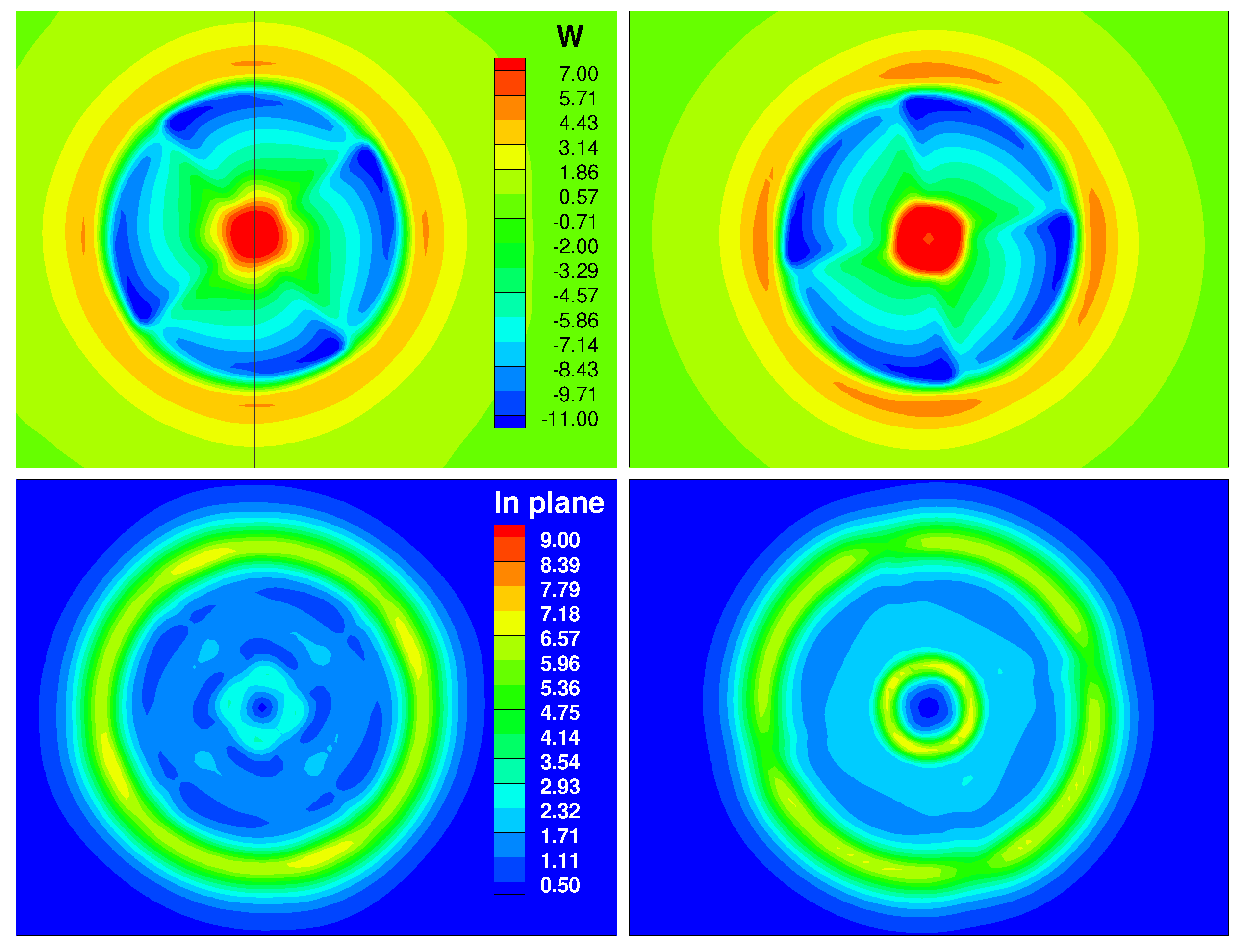
In the viscous option, the shape obtained after the end of the first period (Figure 11b vs. Figure 11a) is very similar to that of the inviscid option. The predicted position of the vortex ring is almost identical in the two sets (see also Table 2). However, the magnitude of the vorticity at the tip in the viscous option is higher and so will be the loading. Higher circulation of the vortex ring implies that also higher down-wash will develop in the wake at the early stages of its generation. In Figure 12, the down-wash and the in-plane velocity components over the rotor disk as obtained with the two modeling options are compared.
Although the differences are small, the down-wash velocities (negative sign) over the rotor disk plane are higher in the viscous case (the extent of the blue pattern is greater in the viscous option results). Furthermore, the up-wash induced velocities are higher by the wake outside the rotor disk area as well as the in-plane velocities within the rotor disk area. This explains why in the viscous option, at the end of the 2nd period, both the vortex ring and the tip vortices of the blades have traveled longer downwards distance as compared to the inviscid case. The same happens at the end of the 3rd revolution (longer downwards distance traveled by the wake) while in addition to the above the ground boundary layer starts to develop. The shear in this boundary layer is caused by the wake jet flow that at the end of the 3rd revolution impinges on the ground. The development of the boundary layer creates a vertical displacement effect (an upwards transpiration velocity related to the displacement thickness of the boundary layer) which affects the shape of the vortex ring. The distortion of the vortex ring in the viscous modeling option begins earlier than in the inviscid one (already at the end of the 3rd revolution). The reason for that is twofold: (i) the ring in the viscous option travels downwards with a higher velocity due to higher loading and (ii) it interacts with the boundary layer of the ground. At the end of the 4th period, the thickness of the boundary layer has further increased while a stronger interaction with the vortex ring is observed. The cross section of the vortex ring obtains an elliptical shape. As a result of getting closer to the ground, its interaction with the boundary layer on the ground gets stronger. The outer edge of the ring is closer to the edge of a thicker boundary layer as compared to the inner edge. Transpiration velocities are therefore higher over the outer edge of the ring and the ring appears to rotate around its axis. At the end of 6th and 10th revolution, the vortex ring moves upwards and away from the ground as if it rebounds (at and , respectively, see Table 2), while wake tip vortices start to interact with the boundary layer on the ground.
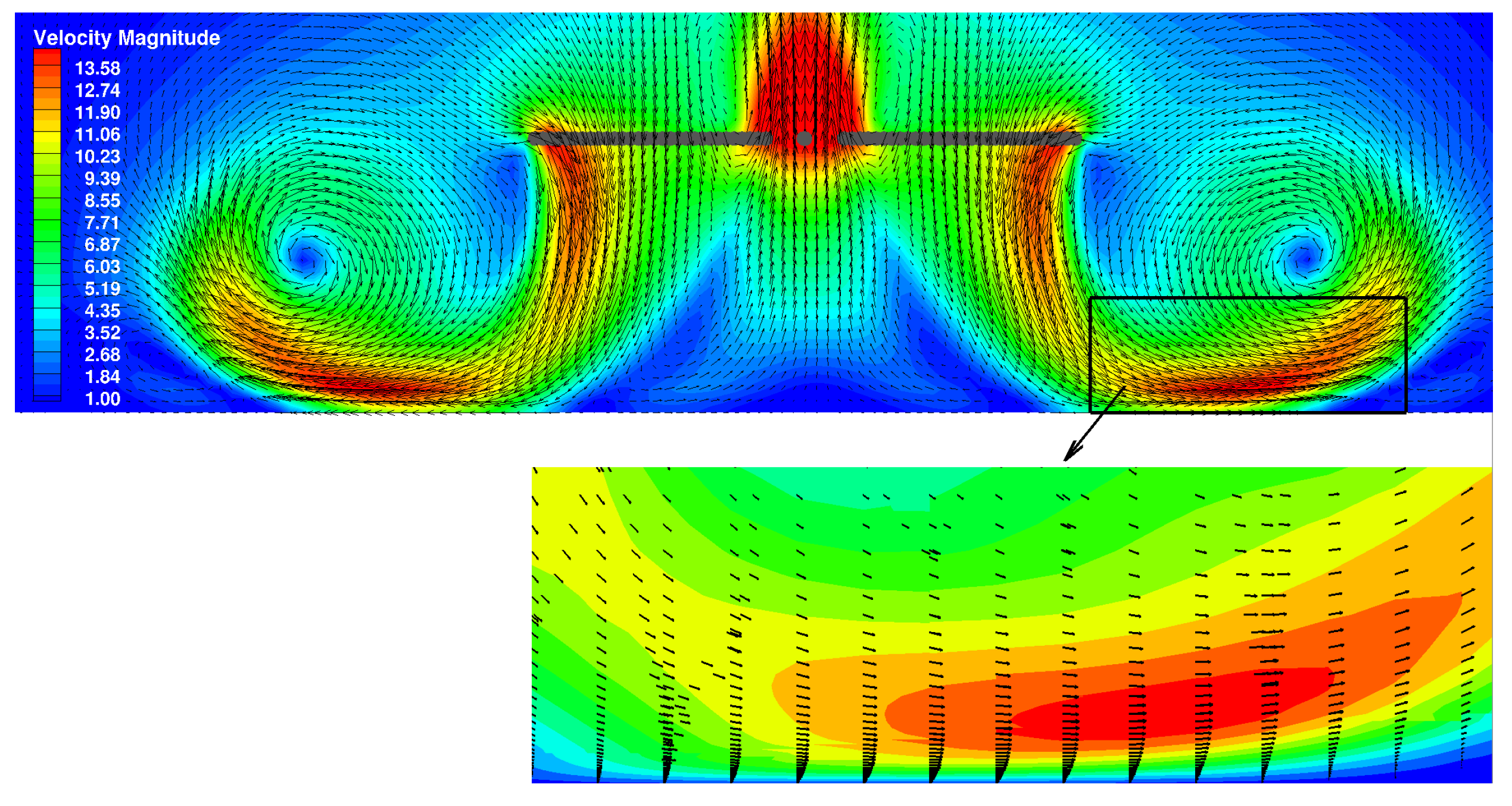
Figure 13 shows the details of the flow field on an axial symmetry plane at the end of the 6th period. The window focuses on the interaction zone of the vortex ring with the boundary layer on the ground. As Table 2 also indicates, at this instant the vortex core is located halfway between the ground and the rotor plane. The recirculating flow of the vortex extends down to the ground level and interacts with the ground boundary layer. In the close-up plot, the anti-clockwise rotating flow of the vortex ring that entrains the boundary layer, is clear (left side of the focus window). Maximum flow velocities are obtained below the vortex center, at a distance from the ground level. The increasing thickness of the boundary layer (right side of the plot) pushes the vortex away from the ground, realizing the so called re-bound effect.
The above comparison has revealed that as the distance from the ground gets smaller, two features that can only be reproduced by taking into account viscosity become decisive: First, the induced velocities in the wake are higher leading to higher loading and secondly, the vortex ring rebounds from the ground pushed by the displacement generated in the ground boundary layer.
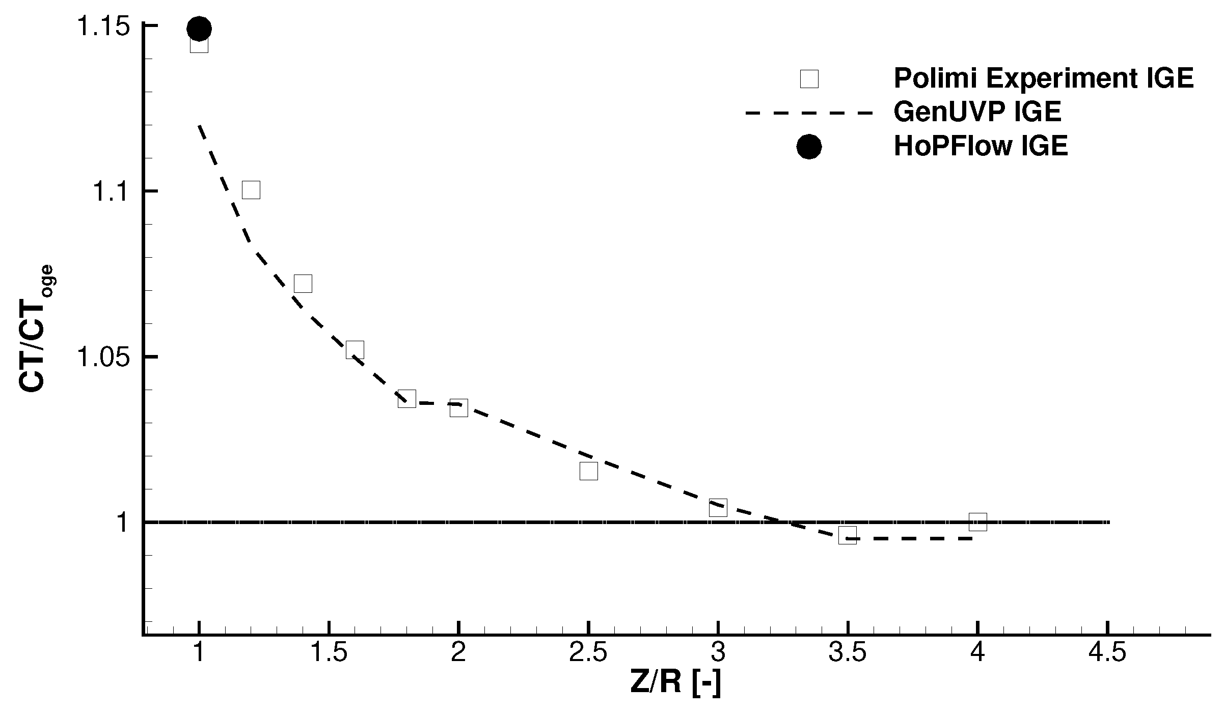
With respect to loading, which was the initial motivation of this work, in Figure 14 the results obtained with the potential flow solver [13] are compared to measurements indicating that at , the agreement is very good. It also captures the “knee” of the variation at . Below there is increasing deviation that becomes maximum at . At this position, predictions with HoPFlow using the viscous option reconfirm the importance of the ground boundary layer by fully recovering the measured value. At , the IGE simulation gives normalized of 1.149 against the 1.144 of the experiment (results are summarized in Table 3), while the inviscid option gives 1.1235 which is very close to the prediction of the free wake code. In these results, normalization is defined with respect to the values provided in Section 4.1.
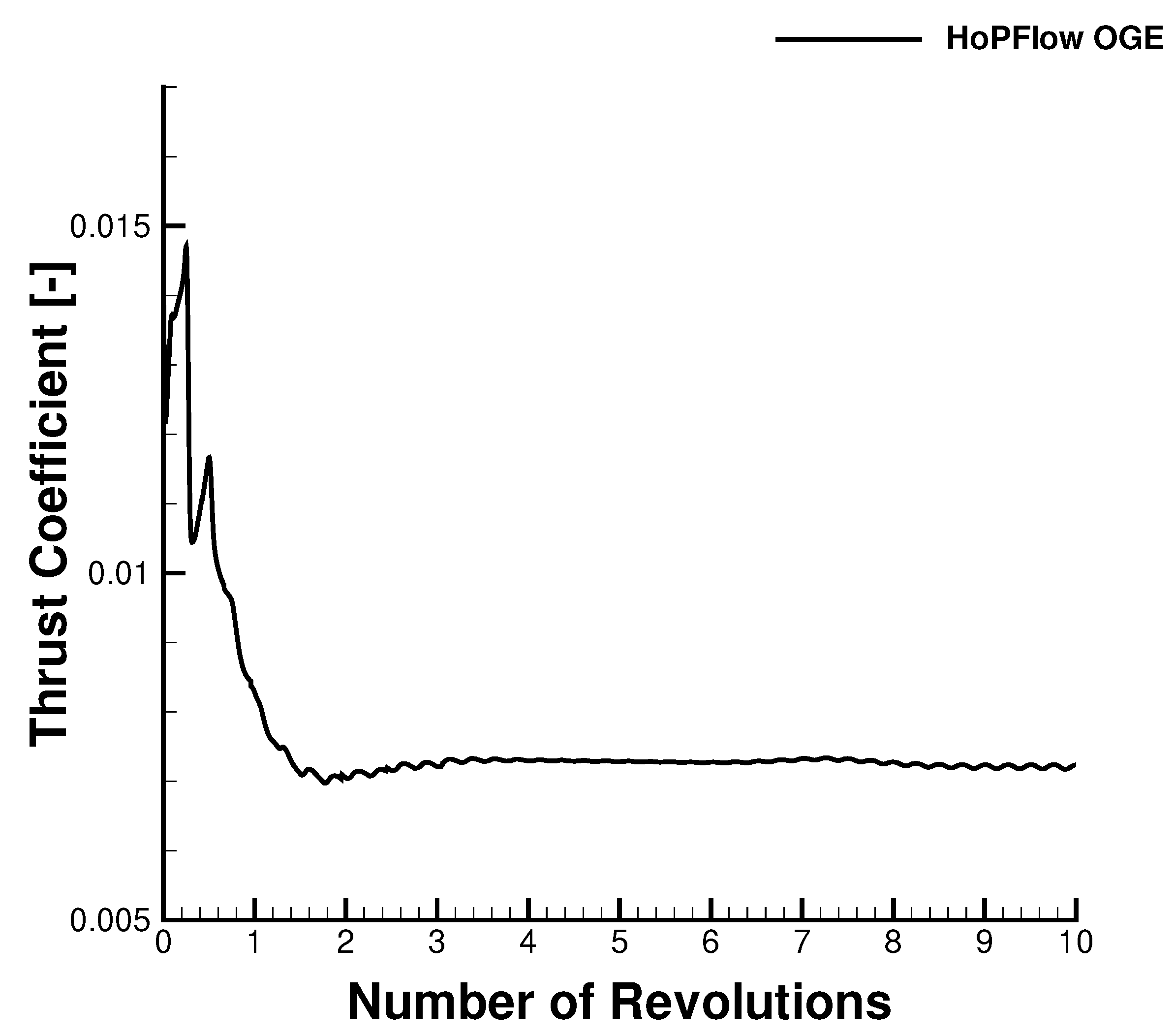
Comparison of the predicted CT time series of the two HoPFlow simulation options shown in Figure 15 for the case , indicates that the presence of a viscous wall gives rise to increased thrust of the rotor already at the very beginning of the simulation while after a number of revolutions CT converges to higher value.
5. Conclusions and Discussion
This paper addresses the near-ground hover flight and attempts to revise earlier potential flow predictions by introducing the effect of flow viscosity in the simulation, in particular the viscous boundary layer that develops on the ground as a result of the rotor down-wash. The simulation environment adopted in this analysis is a hybrid Eulerian–Lagrangian CFD solver which can conveniently accommodate solid bodies that move independently the one from the other. The Eulerian and Lagrangian flow solutions are consistently coupled through properly defined boundary conditions for the Eulerian problem and an iterative scheme, in the course of which the Lagrangian solution (material description of flow quantities over the entire flow domain) is adequately corrected.
The work aimed to (i) identify the physical mechanisms of the rotor/ground interaction in the presence of a viscous boundary layer on the ground, and (ii) prove that a hybrid solver based on particles is capable of consistently predicting OGE and IGE rotor loads. In this connection, simulations of the hybrid Eulerian–Lagrangian solver HoPFlow have been performed for OGE and IGE (close proximity to the ground of one rotor radius) hover flight conditions considering the ground both as an inviscid and a viscous wall. Comparison of HoPFlow rotor thrust predictions for the OGE case and the IGE case with the ground being modeled as an inviscid wall against predictions by the potential free wake GenUVP code indicated an excellent agreement of the two models, which however underestimated the measured increase in thrust by ≈. The above comparison is a verification of HoPFlow predictions but also suggests that the modeling of the ground is of critical importance for the correct account of the rotor ground interactional phenomena and thereby for the accurate prediction of rotor loads in IGE conditions. Besides, the above conclusion was experimentally confirmed by Nathan and Green [5].
HoPFlow predicted the thrust for the IGE hover case with the ground being modeled as a viscous wall perfectly well compared to measurements. Cross-comparison of the flow fields of the two HoPFlow IGE simulations (viscous and inviscid options) suggests that in the presence of the ground a displacement effect is caused, driven by the boundary layer transpiration velocities that pushes the rotor wake and the starting vortex to move upwards. In the inviscid simulation option the starting vortex, after hitting the ground moves parallel to it reaching after 10 rotor revolutions a minimum height of . In the viscous simulation option, the starting vortex moves faster downwards due to higher wake induced velocities and as a result of its interaction with the ground boundary layer reaches a minimum distance of . Then bounces back to a higher height of .
Author Contributions
Conceptualization, T.A. and V.R.; methodology, T.A. and G.P.; validation, T.A.; formal analysis, T.A., V.R. and S.V.; writing—original draft preparation, T.A.; writing—review and editing, T.A., G.P., V.R. and S.V.; visualization, T.A.; supervision, V.R. and S.V. All authors have read and agreed to the published version of the manuscript.
Funding
This research received no external funding.
Institutional Review Board Statement
Not applicable.
Informed Consent Statement
Not applicable.
Data Availability Statement
Acknowledgments
NTUA computations were supported by computational time granted from the Greek Research & Technology Network (GRNET) in the National HPC facility—ARIS—under project “ELASTURB” with ID pr005019_thin. The experimental data have been provided by Garteur.
Conflicts of Interest
The authors declare no conflict of interest.
References
- Key, D. Analysis of army helicopter pilot error mishap data and the implications for handling qualities. In Proceedings of the 25th European Rotorcraft Forum, Rome, Italy, 14–16 September 1999. [Google Scholar]
- Curtiss, H.J.; Sun, M.; Putman, W.; Hanker, E.J. Rotor Aerodynamics in Ground Effect At Low Advance Ratios. J. Am. Helicopter Soc. 1984, 29, 48–55. [Google Scholar] [CrossRef]
- Boer, J.; Hermans, C.; Pengel, K. Helicopter Ground Vortex: Comparison of Numerical Predictions with Wind Tunnel Measurement; National Aerospace Laboratory NLR: Amsterdam, The Netherlands, 2001. [Google Scholar]
- Ganesh, B.; Komerath, N. Unsteady Aerodynamics of Rotorcraft in Ground Effect. In Proceedings of the Fluid Dynamics Meeting, Reno, NV, USA, 10–13 January 2005. [Google Scholar]
- Nathan, N.D.; Green, R. The flow around a model helicopter main rotor in ground effect. Exp. Fluids 2012, 52, 151–166. [Google Scholar] [CrossRef]
- Sugiura, M.; Tanabe, Y.; Sugawara, H.; Matayoshi, N.; Ishii, H. Numerical Simulations and Measurements of the Helicopter Wake in Ground Effect. J. Aircr. 2017, 54, 209–219. [Google Scholar] [CrossRef]
- Sugiura, M.; Tanabe, Y.; Sugawara, H.; Barakos, G.; Matayoshi, N.; Ishii, H. Validation of Cfd Codes for the Helicopter Wake in Ground Effect. In Proceedings of the European Rotorcraft Forum, Milan, Italy, 12–15 September 2017. [Google Scholar]
- Cavallo, S.; Ducci, G.; Barakos, G.; Gibertini, G. CFD Analysis of Helicopter Wakes in Ground effect. In Proceedings of the European Rotorcraft Forum, Delft, The Netherlands, 18–21 September 2018. [Google Scholar]
- Pasquali, C.; Serafini, J.; Bernardini, G.; Milluzzo, J.; Gennaretti, M. Numerical-experimental correlation of hovering rotor aerodynamics in ground effect. Aerosp. Sci. Technol. 2020, 106, 106079. [Google Scholar] [CrossRef]
- Visingardi, A.; De Gregorio, F.; Schwarz, T.; Schmid, M.; Bakker, R.; Voutsinas, S.; Gallas, Q.; Boisard, R.; Gibertini, G.; Zagaglia, D.; et al. Forces on obstacles in rotor wake—A GARTEUR action group. In Proceedings of the 43rd European Rotorcraft Forum, Milan, Italy, 12–15 September 2017. [Google Scholar]
- Gibertini, G.; Grassi, D.; Parolini, C.; Zagaglia, D.; Zanotti, A. Experimental investigation on the aerodynamic interaction between a helicopter and ground obstacles. Proc. Inst. Mech. Eng. Part G J. Aerosp. Eng. 2015, 229, 1395–1406. [Google Scholar] [CrossRef] [Green Version]
- Zagaglia, D.; Giuni, M.; Green, R.B. Rotor-obstacle aerodynamic interaction in hovering flight: An experimental survey. Annu. Forum Proc.-AHS Int. 2016, 1, 356–364. [Google Scholar]
- Andronikos, T.; Papadakis, G.; Riziotis, V.; Prospathopoulos, J.; Voutsinas, S. Validation of a cost effective method for the rotor-obstacle interaction. Aerosp. Sci. Technol. 2021, 113, 106698. [Google Scholar] [CrossRef]
- Voutsinas, S.G. Vortex methods in aeronautics: How to make things work. Int. J. Comput. Fluid Dyn. 2006, 20, 3–18. [Google Scholar] [CrossRef]
- Schmid, M. Simulation of helicopter aerodynamics in the vicinity of an obstacle using a free wake panel method. In Proceedings of the 43rd European Rotorcraft Forum, CEAS, Milan, Italy, 12–15 September 2017. [Google Scholar]
- Papadakis, G. Development of a Hybrid Compressible Vortex Particle Method and Application to External Problems Including Helicopter Flows. Doctoral Dissertation, National Technical University of Athens, Athens, Greece, 2014. [Google Scholar]
- Papadakis, G.; Voutsinas, S.G. A strongly coupled Eulerian Lagrangian method verified in 2D external compressible flows. Comput. Fluids 2019, 195, 104325. [Google Scholar] [CrossRef]
- Roe, P.L. Approximate Riemann solvers, parameter vectors, and difference schemes. J. Comput. Phys. 1981, 43, 357–372. [Google Scholar] [CrossRef]
- Venkatakrishnan, V. On the Accuracy of Limiters and Convergence to Steady State Solutions. In Proceedings of the On the Accuracy of Limiters and Convergence to Steady State Solutions, Reno, NV, USA, 11–14 January 1993. [Google Scholar]
- Spalart, P.; Allmaras, S. One-Equation Turbulence Model for Aerodynamic Flows. Rech. Aerosp. 1994, 5–21. [Google Scholar] [CrossRef]
- Menter, F. Zonal Two Equation k-omega Turbulence Models for Aerodynamic Flows. In Proceedings of the 23rd Fluid Dynamics, Plasmadynamics, and Lasers Conference, Orlando, FL, USA, 6–9 July 1993. [Google Scholar]
- Ghosal, S. An analysis of numerical errors in large-eddy simulations of turbulence. J. Comput. Phys. 1996, 125, 187–206. [Google Scholar] [CrossRef] [Green Version]
- Spyropoulos, N.; Prospathopoulos, J.; Manolas, D.; Papadakis, G.; Riziotis, V.A. Development of a fluid structure interaction tool based on an actuator line model. J. Phys. Conf. Ser. 2020, 1618, 052072. [Google Scholar] [CrossRef]
- Schmitz, S.; Chattot, J.J. A coupled Navier–Stokes/Vortex–Panel solver for the numerical analysis of wind turbines. Comput. Fluids 2006, 35, 742–745. [Google Scholar] [CrossRef]
- Martinez-Tossas, L.; Churchfield, M.; Leonardi, S. Large eddy simulations of the flow past wind turbines: Actuator line and disk modeling. Wind Energy 2015, 18, 1047–1060. [Google Scholar] [CrossRef]
- Jha, P.; Schmitz, S. Actuator curve embedding—An advanced actuator line model. J. Fluid Mech. 2018, 834. [Google Scholar] [CrossRef]
- Troldborg, N.; Sørensen, N.N.; Michelsen, J. Numerical simulations of wake characteristics of a wind turbine in uniform inflow. Wind Energy 2010, 13, 86–99. [Google Scholar] [CrossRef]
- Beale, J.T.; Majda, A. Higher order accurate vortex methods with explicit velocity kernels. J. Comput. Phys. 1985, 58, 188–208. [Google Scholar] [CrossRef]
- Cottet, G.H.; Koumoutsakos, P. Vortex Methods: Theory and Practice; Cambridge University Press: Cambridge, UK, 2000. [Google Scholar]
- Wang, K.; Riziotis, V.A.; Voutsinas, S.G. Aeroelastic stability of idling wind turbines. Wind Energy Sci. 2017, 2, 415–437. [Google Scholar] [CrossRef] [Green Version]
Figure 1.
Velocity triangle and aerodynamic loads on a blade section. Actuator line analysis definitions.
Figure 1.
Velocity triangle and aerodynamic loads on a blade section. Actuator line analysis definitions.

Figure 2.
The Eulerian domain contains the solid boundary . The Lagrangian domain includes and and .
Figure 2.
The Eulerian domain contains the solid boundary . The Lagrangian domain includes and and .

Figure 3.
Spatial distribution of the E- particles. (Left): One E-cell is shown within a 4 × 4 stencil of the PM grid corresponding to the projection function. There are four particles in the E-cell marked as blue circles. (Right): A part close to the solid boundary is shown. On , surface particles are shown as blue open circles. The middle surface particle is embedded in the stencil activated for its projection.

Figure 4.
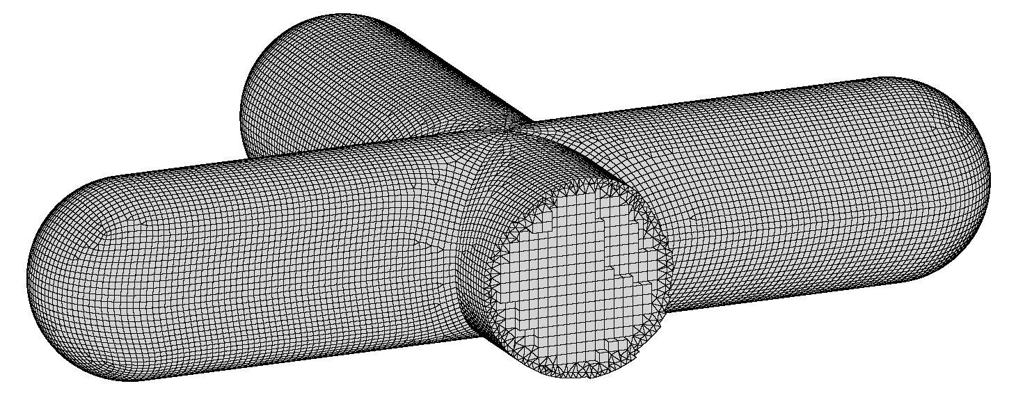
CFD meshes surrounding the rotor blades. Red lines represent the blades.

Figure 5.
CFD mesh cut at a specific radial station of the blade.

Figure 6.
CFD mesh around the actuator line and the ground.

Figure 7.
Velocity magnitude and vectors of the OGE case over an axi-symmetry plane (snapshot at the end of the 10th period).
Figure 7.
Velocity magnitude and vectors of the OGE case over an axi-symmetry plane (snapshot at the end of the 10th period).

Figure 8.
Trailing tip and root vortices at an early stage of the simulation.

Figure 9.
Trailing tip and root vortices after 10 rotor revolutions.

Figure 10.
Thrust coefficient convergence in OGE conditions. Predictions of HoPFlow.

Figure 11.
Vorticity contour plots for the IGE case at (snapshots taken at the end of the 1st, 2nd, 3rd, 4th, 6th, and 10th rotor revolution). Inviscid ground condition (left), viscous ground condition (right).
Figure 11.
Vorticity contour plots for the IGE case at (snapshots taken at the end of the 1st, 2nd, 3rd, 4th, 6th, and 10th rotor revolution). Inviscid ground condition (left), viscous ground condition (right).

Figure 12.
Comparison of the vertical and in-plane velocities at the level of the rotor (). Inviscid condition on the ground (left) and viscous condition (right).
Figure 12.
Comparison of the vertical and in-plane velocities at the level of the rotor (). Inviscid condition on the ground (left) and viscous condition (right).

Figure 13.
Snapshot of flow field (velocity magnitude and vectors) over an axi-symmetry plane at , when viscous wall conditions are applied (snapshot at the end of the 6th period).
Figure 13.
Snapshot of flow field (velocity magnitude and vectors) over an axi-symmetry plane at , when viscous wall conditions are applied (snapshot at the end of the 6th period).

Figure 14.
Normalized thrust coefficient in IGE conditions. Comparison of predictions with GenUVP and HoPFlow against measurements.
Figure 14.
Normalized thrust coefficient in IGE conditions. Comparison of predictions with GenUVP and HoPFlow against measurements.

Figure 15.
Rotor thrust variation in IGE condition at . Comparison of HoPFlow predictions for the inviscid wall case against the viscous wall.
Figure 15.
Rotor thrust variation in IGE condition at . Comparison of HoPFlow predictions for the inviscid wall case against the viscous wall.


Table 1.
OGE thrust coefficient comparison of measured data against predictions (convergent values after 10 rotor revolutions).
Table 1.
OGE thrust coefficient comparison of measured data against predictions (convergent values after 10 rotor revolutions).
| Measured Thrust Coefficient | Predictions GenUVP | Predictions HoPFlow |
|---|---|---|
| 0.007270 | 0.007290 | 0.007285 |
Table 2.
Comparison of IGE values of vortex ring center location for hover flight at .
| Period | [Z/R] Inviscid Wall | [r/R] Inviscid Wall | [Z/R] Viscous Wall | [r/R] Viscous Wall |
|---|---|---|---|---|
| 1st | 0.98 | 1.02 | 0.985 | 1.02 |
| 2nd | 0.80 | 1.08 | 0.79 | 1.07 |
| 3rd | 0.58 | 1.18 | 0.53 | 1.19 |
| 4th | 0.45 | 1.34 | 0.39 | 1.41 |
| 6th | 0.28 | 1.76 | 0.51 | 1.86 |
| 10th | 0.22 | 2.14 | 0.65 | 2.00 |
Table 3.
Comparison of IGE values of at .
| Experiment | Inviscid Wall | Viscous Wall | GenUVP |
|---|---|---|---|
| 1.1441 | 1.1235 | 1.149 | 1.121 |
Publisher’s Note: MDPI stays neutral with regard to jurisdictional claims in published maps and institutional affiliations. |
© 2021 by the authors. Licensee MDPI, Basel, Switzerland. This article is an open access article distributed under the terms and conditions of the Creative Commons Attribution (CC BY) license (https://creativecommons.org/licenses/by/4.0/).
Share and Cite
MDPI and ACS Style
Andronikos, T.; Papadakis, G.; Riziotis, V.; Voutsinas, S. Revising of the Near Ground Helicopter Hover: The Effect of Ground Boundary Layer Development. Appl. Sci. 2021, 11, 9935. https://0-doi-org.brum.beds.ac.uk/10.3390/app11219935
AMA Style
Andronikos T, Papadakis G, Riziotis V, Voutsinas S. Revising of the Near Ground Helicopter Hover: The Effect of Ground Boundary Layer Development. Applied Sciences. 2021; 11(21):9935. https://0-doi-org.brum.beds.ac.uk/10.3390/app11219935
Chicago/Turabian StyleAndronikos, Theologos, George Papadakis, Vasilis Riziotis, and Spyros Voutsinas. 2021. "Revising of the Near Ground Helicopter Hover: The Effect of Ground Boundary Layer Development" Applied Sciences 11, no. 21: 9935. https://0-doi-org.brum.beds.ac.uk/10.3390/app11219935
Note that from the first issue of 2016, this journal uses article numbers instead of page numbers. See further details here.