Article

Exploring the Benefits of Photovoltaic Non-Optimal Orientations in Buildings

by
Esteban Sánchez
1,*,
Ángel Ordóñez
1,2,
Alberto Sánchez
3,
Raúl García Ovejero
3,4 and
Javier Parra-Domínguez
5
1
Electronic Technology Area, E.T.S.I.I Béjar, University of Salamanca, Avda. Fernando Ballesteros, 2, Béjar, 37700 Salamanca, Spain
2
Facultad de la Energía, Universidad Nacional de Loja, Avda. Reinaldo Espinoza, Loja 110110, Ecuador
3
Department of Mechanical Engineering, E.T.S.I.I Béjar, University of Salamanca, Avda. Fernando Ballesteros, 2, Béjar, 37700 Salamanca, Spain
4
Expert Systems and Applications Lab, E.T.S.I.I Béjar, University of Salamanca, 37008 Salamanca, Spain
5
Department of Business and Economics Administration, E.T.S.I.I Béjar, University of Salamanca, Avda. Fernando Ballesteros, 2, Béjar, 37700 Salamanca, Spain
*
Author to whom correspondence should be addressed.
Submission received: 21 September 2021 / Revised: 14 October 2021 / Accepted: 19 October 2021 / Published: 25 October 2021

Abstract

:

Featured Application

This work is intended to be used as a reference for designing photovoltaic installations in buildings which do not have architectural surfaces with optimal orientations or when it is required the use of several surfaces for maximizing total energy production.

Abstract

As solar photovoltaics in buildings reaches maturity, grid integration and economic yield are topics of greater interest. The traditional design of photovoltaic installations has considered the optimal orientation of photovoltaic modules to be that which yields the maximum annual energy production. The influence of the consumption patterns and the hourly variable electricity prices implies that this traditional optimal design might not be the most profitable. Using a full-year dataset for a residential installation, alternative installations using canopies and modules attached to the façades are simulated. By evaluating the energy balances for different annual consumptions, it is found that the canopy and façade installations offer better self-consumption of the PV produced energy, reflected in a 9% higher self-consumption degree using modules on façades and a 5% higher self-consumption degree using canopies. The economic evaluation under the new electricity tariffs in Spain shows a better profit for PV self-consumption, reducing the time of return on investment by more than 2 years. The analysis of different alternatives for an industrial PV allowed us to identify several benefits for these orientations which are confirmed after a full year of operation, such as an increase of up to 59% in annual energy production over the optimal-producing orientation.

1. Introduction

Economic growth and rising global living standards generate a continuous increase in energy demand; by 2050, this growth is expected to be responsible for an energy consumption of approximately 1.5 to 3 times the current level [1,2]. To meet this demand, renewable energies, mainly wind and solar, are presented as a technically feasible and socially accepted alternative [3,4], and this trend of growth of this type of energy sources is clearly seen in the numerous projects that have been and are being designed for their implementation [5]. In addition to the advantages of this type of energy, there is a fundamental condition for its expansion, which is that CO2 emissions must be lowered in order to achieve its climate change objectives [6]. Given these circumstances, it is estimated that, by 2050, the amount of oil and coal used in the energy mix will have more than halved from current levels, and the energy supply mix will be equally divided between renewable and non-renewable sources [7].
Within renewable energies, the breakthrough in solar energy is mainly due to increased efficiency and continued cost reductions [8,9], and this has led to a worldwide growth in installed solar photovoltaic (PV) capacity [10], increasing by 104% in Europe from 2019 according to SolarPower Europe [11]. In 2020, a year that has been affected by the pandemic, the installed capacity has increased by 11% compared to 2019, reaching 18.2 GW, establishing it as the second best year for PV in Europe, second only to the solar boom in 2011 when 21.4 GW were installed [12]. Spain’s current situation in the European environment places is ranked fourth in terms of installed solar capacity, far behind Germany, which is the undisputed leader with more than 48 GW of installed solar capacity. In addition, it also ranks third in terms of solar contribution to total generation in each country, after Germany, which leads the ranking, and Greece. Specifically, 2931 MW were installed in Spain in 2020, reaching a total figure of 11,714 MW, which is equivalent to approximately 11% of total capacity and close to 20% of renewable power. Of these figures, 596 MW of photovoltaic capacity corresponds to self-consumption, where 19% represented domestic self-consumption, nine points above the progress recorded in 2019. The future of photovoltaics in Spain has major goals, which have been consolidated in the National Integrated Energy and Climate Plan 2021–2030 (PNIEC) [13], which proposes a 100% renewable electricity sector by 2050, with an intermediate stage of 74% by 2030. It also adds among its goals to reach a total installed capacity of 44 GW of solar energy by 2030, of which 37 GW will be photovoltaic.
In the study of solar installations in buildings, there are two main ways of incorporating PV technology into a building: building-attached photovoltaics (BAPV) and building-integrated photovoltaics (BIPV). In BAPV systems, the PV modules are installed by anchoring them to the building and in BIPV systems, and are part of the building façade, i.e., they serve as building material in the building envelope as multifunctional elements [14]. BIPV is considered one of the four key factors essential for the future success of photovoltaics. However, the power generation efficiency of BIPV systems is lower compared to current stand-alone PV systems, up to 41% due to irradiation loss alone [15], although it has the advantages of eliminating the additional space needed for power generation and presenting better aesthetics for the building structure [16]. Therefore, studies of the electrical efficiency of self-consumption in a building with solar generation are mainly based on BAPV systems.
These electrical efficiency studies are conducted based on achieving near-zero energy buildings (NZEB) and grid parity [17]. This occurs when PV electricity costs are equal to the retail electricity price, considering fixed factors such as revenue, savings, implementation costs, maintenance costs, taxes and depreciation, and other variable factors (such as investment costs, credit discount rate, and variations in the retail electricity price that complicate the calculation to reach grid parity, which pose a scenario that requires economic incentives and support policies) [18]. These are the reasons why some solar markets are called mature, such as Germany and Italy, when reaching grid parity [18,19]. Spain has recently reached grid parity [20] aided by the recent approval of Royal Decree 244/2019 [21], which develops the administrative, technical, and economic conditions of Royal Decree Law 15/2018 [22]. The new regulation introduces a simplified compensation mechanism in the electricity bill for consumers, following a net-billing scheme [23].
Regardless of the photovoltaic strategy selected, the analysis carried out by [24] outlines the features of the energy production of PV modules placed in a different orientation to the optimal energy-producing one. Due to the limited roof area available for placing PV, a strategy for increasing the electricity production of photovoltaic self-consumption systems (PVSCS hereinafter) is to place PV modules in suitable façades. For example, it is showed in [24] that, for buildings with administrative or office uses, an installation facing southeast provides a better fit for electricity consumption, which is higher in the morning [25]. This presents us with scenarios where installing solar panels in non-optimal orientations is possible to obtain a potential benefit. These scenarios would produce lower amounts of energy, but their hourly production profiles could shift beyond noon, allowing them to better meet demand [26,27].
The main objective of the presented research is to analyze the technical and eco-nomic potential of the integration of PVSCS in non-optimal orientations in Spain, using reference installations with real consumption and PV production. For reaching this goal, the analysis of two case studies is carried out on a residential and an industrial PVSCS. Based on one full year of real operational data for the residential PVSCS, the operation of several alternative PV arrangements suitable for the building using different orientations are simulated and an energy and economic analysis is carried out considering past and new residential tariffs in Spain. For the investigation on industrial PVSCS, the reference case is a mid-size installation of 169 kW using orientations different from the South. It is shown the analysis of different layouts for the PV modules prior to the project that led to the use of this orientation. Due to the recent construction of this PVSCS, preliminary results are presented.
Thus, the paper is divided as follows. After the introduction, Section 2 describes the case studies, with a description of Spanish residential tariffs and the methods used in the energy and economic analysis of energy consumption and production for each case study. Section 3 presents the results of both case studies, with including an economic analysis for the different configurations evaluated in the residential PVSCS, which will then be discussed in Section 4. Finally, in Section 5, the conclusions are presented.
The main findings of our study are that non-optimal orientations show fair economic performance in residential PVSCS despite their lower energy production. For one alter-native installation using canopies, the economic savings are close to the optimal energy producing, and, for another installation using modules attached to the façade, the eco-nomic benefit is only 14% lower. The new electricity tariffs in Spain will have a positive impact on residential PVSCS economic performance, and will improve by 12%. For industrial applications, these orientations have the potential of installing more PV power, resulting in an increased energy production of 59% for the case study.

2. Materials and Methods

The study of performance of PV installations using PV modules in non-optimal orientations was based on two PVSCS: residential and industrial. The residential PVSCS is on a single-family detached home. Based on the data available from the operation and monitoring of this PVSCS, alternative PV configurations in non-optimal orientations and suitable with the building are proposed and a techno-economic analysis is carried out, studying the viability of the different configurations in comparison with the optimal energy-producing one. The industrial PVSCS corresponds to a factory expansion which was built with a flat roof for installing solar PV, allowing different layouts for the PV modules. Several layouts were considered, and the energy analysis was performed to select the best option exposed.

2.1. Simulation with PVSYST Software

The work presented here uses simulations with this software package, so it will be described in some detail. PVSYST [28] is a reference software widely used in industry and research [29] that reproduces the electrical behavior of a PV module under any conditions (irradiance, temperature of cell, incidence angle, and spectral contents). The simulator is based in the one-diode model for crystalline Si cells and extended to the complete module, described in Equation (1). A complete description of the use in PVSYST can be found in [30]. PVSYT provides an accurate set of parameters for a wide number of PV modules from 2002 to present time.
I = I Φ I 0 e q V + I · R S N C S · γ k T C 1 V + I · R S R S h
where
I ,   V : current and voltage of module;
T C : temperature of cell;
I Φ : photocurrent at measured irradiance G meas ;
I 0 : diode saturation current;
R S : series resistance;
R S h : shunt resistance;
γ : diode ideality factor;
q : charge of the electron;
N C S : number of cells in series in the module.
While the accurate simulation of PV modules and systems depends on a good physical model and an accurate set of parameters, a high-quality energy yield prediction depends also on the environmental parameters [31]. The most important one is the incident irradiance on the module, i.e., the output power proportional to it for a wide range of irradiances. Solar cells are very sensitive to temperature, as can be deduced from Equation (1). In fact, the power of a crystalline silicon PV module decreases significantly with the temperature (typically between −0.3 and −0.4 %/K). The cell temperature depends on the incident irradiation, the ambient temperature, and the windspeed.
In this way, excellent weather datasets are needed. The most accurate method to obtain irradiance measurements (global horizontal and diffuse) is with ground radiometers, with a sparse coverage. Actual databases are built to integrate data from ground radiometers and satellite-based models [32]. In this work, Meteonorm and PVGIS-SARAH databases were used. The Meteonorm database [33] uses ground data from the Global Energy Balance Archive data [34], provided from national weather services and data from 5 geostationary satellites where no radiation measurement is available nearer than 30 km (10 km in Europe). The data correspond to the periods 1981–1990 and 1996–2015. The PVGIS-SARAH database [35] uses data from two EUMETSAT geostationary satellites and provides long-term averages calculated from the period 2005–2016. These datasets also include hourly data of ambient temperature and windspeed. The data from the datasets were used to generate a typical meteorological year, containing one year of hourly data that represent median weather over a multiyear period. The irradiation data (global and diffuse) allow a calculation of irradiance on inclined surfaces. If diffuse irradiation is not available, PVSYST uses the Erbs correlation model [
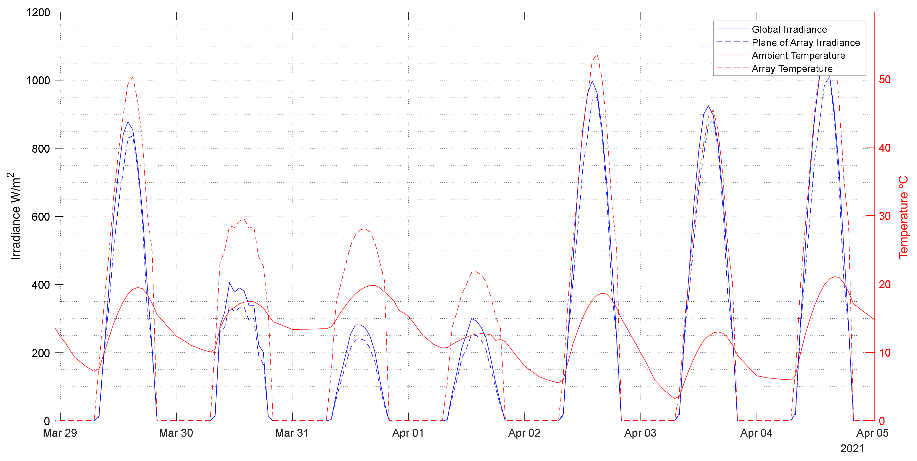
36] for calculation. In Figure 1, the irradiances and temperatures of one the PVSCS simulated in this work are shown. It can be noted that the module temperature is only calculated when the irradiance is higher than zero. This software was compared with other software packages (HOMER, RETScreen) and was found to be accurate while also providing conservative energy estimations compared with the aforementioned [37].
An important feature of PVSYST software is that it includes a 3D design tool for calculating the shading scene according to the sun trajectories along the year. The impact of shadings in the calculation can be selected as: “none”; “linear”, derating of the output power according with the shaded area; derating “according with the strings configuration”; and “electrical detailed calculation”, according to the bypass diodes in the module.

2.2. Case Study #1: Residential PVSCS

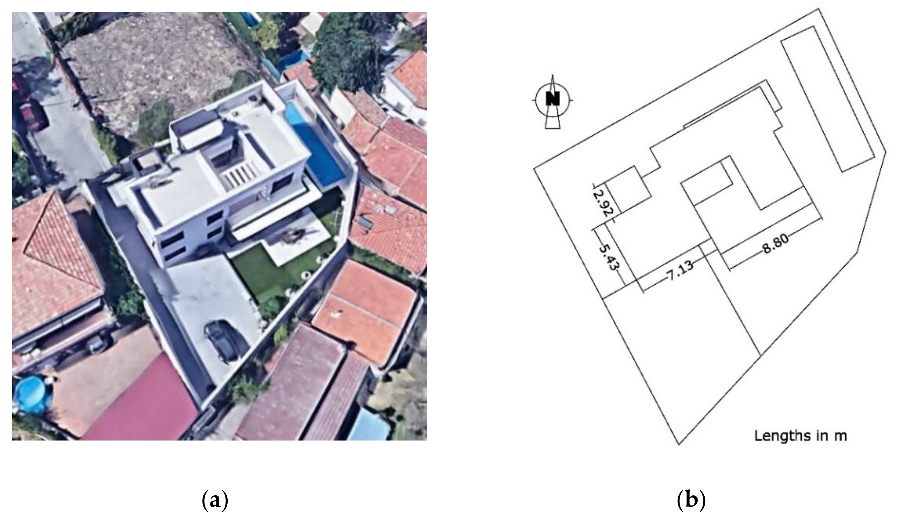
The residential PVSCS is a single-home building located in the Madrid metropolitan area (40°27′ N, 3°48′ W). It is a two-story detached building equipped with heating and ventilation air conditioned (HVAC), as shown in Figure 2 [38]. The climate in Madrid is continental Mediterranean, with cold winters and hot summers. Hence, the yearly consumption is high, 14,189 kWh for the full-year period under study. The installation has a peak power of 3.85 kW and uses 10 Canadian Solar Ku Max CS3U-385MS monocrystalline PERC PV modules with power optimizers connected in a single string to a 4-kW SolarEdge inverter. The modules are installed on the roof, with a southeast orientation aligned with the building and with an inclination of 30°.
The methodology used for the analysis is as follows. Using the reference building, several suitable alternative PVSCS with non-optimal energy-producing orientation were simulated with PVSYST. The energy balances with the grid were calculated using the original installation energy consumption data. Then, the economic balance was performed using the electricity prices for the energy imported and exported from the grid under Spanish regulation. This economic balance served as the cashflow for the financial study.
The biggest issue when comparing the performance of these different orientations was that the annual production varies for each case. Different annual PV production is the result of different instantaneous PV power; this means that, as the electricity consumption is the same, the balance of self-consumption and surplus are different, affecting the economic results. In fact, for a less-producing layout, there would be a higher share of self-consumption and a lower proportion of surplus energy. As long as self-consumed electricity is valuated at retail price and the surplus near at wholesale price, the less-producing layouts economic results would be overestimated.
The method that was used for a proper comparison. For all the different layouts, the former PVSYST simulations results were rescaled for yearly productions between 5000 kWh and 15,000 kWh, and the energy and economic balances were performed. In this way, there would be a better comparison, and the effects of the different hourly PV production profiles of each layout would be distinguished.

2.2.1. Description of the Alternative PVSCS Layouts

This PVSCS was built in a single-home detached building with no important shadings from nearby constructions, so there were several options for installing a PVSCS on it. The orientation was 30° E for the larger façade and 60° W for the shorter one. The roof was flat, and was divided into two sections connected through a corridor. The owners decided to install the PV modules on the southern part of the roof in two rows of 5 modules each with portrait orientation, as is shown in Figure 3a. For this study, three alternatives are considered: the first one uses canopies with an inclination of 30° on the southeast and southwest façades, as shown in Figure 3b; the second one uses modules attached over the same façades, as shown in Figure 3c; and the third is mixed, using a canopy on the southeast façade and modules attached on the southwest façade.
The original PVSCS uses power optimizers (one for each PV module), and they are connected to the inverter in a single-string configuration. For the other options, a single-string configuration is also possible, but two strings are preferred. In this case, a minimum length of 6 modules was mandatory for this inverter and power optimizers. It is important to note that, for the two orientations configurations, the peak power was flattened so the inverter can easily accommodate the sum of both strings. These inverters can drive a peak power (DC) up to 50% higher than the nominal AC output. Thus, the cost of the alternatives using several orientations is only increased by the additional modules needed.
The original PVSCS, the three alternative layouts, and the energy optimal one are simulated using PVSYST 7.1 [28,39]. This software provides the results on an hourly basis. The meteorological database used for this location was the Meteonorm 7.3 because it is near Madrid, and the models for the PV modules and the SolarEdge P405 power optimizers and SE4000H inverter were provided with the software. Thermal parameters, mismatch, and incidence angles were selected by default. No ageing degradation was used in the simulations because a 0.8% linear degradation was assumed in the financial analysis. The simulations were performed using the detailed electrical model considering the design of the module.

2.2.2. Energy Balances

The PVSCS was installed in February 2020, so there were data for a full year, starting in March 2020. As electricity prices are rising in 2021 after the low prices during the COVID-19 pandemic, the period under study was selected from August 2020 to July 2021. The monitoring system provides data of the PV-produced electricity E P V , consumed electricity E , self-consumed PV electricity E s c , and the exchanges with the grid (energy imported: E i n , exported: E s r p l ) every fifteen minutes. The relationships between these energies are expressed in Equations (2) and (3).
E = E i n + E P V E s r p l
E s c = E P V   i f   E > E P V E s c = E   i f   E < E P V
It is important to take note of the period used for the energy calculation in Equations (2) and (3) which can affect the results of the energy imported and exported to the grid when calculated from the energy consumed and PV produced. It is shown that time averaging of the instantaneous powers has a small effect on export proportions for mid-range generation levels (of the order of the average house demand), but a larger effect on import proportion [40]. An optimal 5-min period was proposed as a solution of compromise. This topic is further investigated in [41] and it is found that even a 5-min period can give noticeable errors over a 1-min period due to the variability of home appliance loads and due to some rapid variations of irradiance. As long as the PV systems under study measures the PV production and both the imported and exported energy, there is no error in the energy consumed even with fluctuations in the consumption and/or PV production.
These data, aggregated in hourly periods, serve as a reference for comparison with simulations of alternative installations with the modules in different orientations suitable with the building.
The simulated energy production E P V was processed with the measured consumption profile E . Using Equations (2) and (3), the PV self-consumed energy E s c , the surplus energy fed into the grid E s r p l , and the energy imported from the grid E i n were computed. In addition, the self-consumption and self-sufficiency degrees are calculated as defined in [42] and expressed in Equations (4) and (5).
S C D = S e l f c o n s u m p t i o n = E P V E s r p l E P V
S S D = S e l f s u f f i c i e n c y = E P V E s r p l E i n + E P V E s r p l
Once the energy balances were calculated, the next step is the calculation of the economic balances. The energy costs saved represent the valuation of the self-consumed PV energy at the hourly retail price of electricity. The surplus energy is valuated at a price slightly lower than the wholesale electricity market hourly price.
Regarding the electricity prices, the Spanish electrical grid operator Red Eléctrica de España (REE) provides real-time information about electricity pricing and a valuation of surplus electricity for PVSCS in its webpage ESIOS [43]. With the processed data, it is possible to compute the economic savings under Spanish self-consumption regulation [21] and the residential pricing of electricity, which will be addressed in the next subsection.

2.2.3. Residential Tariffs in Spain

Before performing the economic evaluation, the residential tariffs for electricity in Spain need to be looked at. These tariffs are composed of three parts: a part based on the nominal contracted power (named access charge), a variable part for the energy consumed (energy charge), and taxes (a 5.11% of electricity tax and 21% VAT, resulting in a total of 27.50%). The final price of the electricity for the consumer depends on the electricity marketer company and the consumer can freely choose among a variety of commercial offers in the free market and in the regulated marked.
The electricity tariffs not only support the costs of the production, transport, and distribution of the electricity. The costs of producing electricity exhibit in the wholesale electricity market prices. In Spain, the overall costs of the electrical system are called tolls and charges. Tolls include the electricity transport and distribution costs and are established by the National Commission for Markets and Competition (CNMC). Charges are a concept, including other costs such as renewable energy retribution (mainly the FiT for wind and solar power generation, overcharges of the Balearic and Canary Island electrical systems, tariff deficit, and other costs). The charges are established by the national government. Part of these costs are included in the access charge and part in the energy charge. For residential tariffs, there are no other charges, such as reactive power and maximum demand penalties. The maximum power demanded for these consumers is controlled by the ICP, which is a switch that turns off the electricity supply if the maximum contracted power is exceeded in a 15-min period. So, the installation of a self-consumption system does not allow a reduction in the contracted power for the residential case. A more comprehensive description of the Spanish tariffs is available in [44].
Formerly, there were three main residential tariffs of choice in the regulated market or PVPC (voluntary price for the small consumer).
  • Time constant tariff: the price of electricity is indexed to the pool market by a fixed toll that includes part of the electrical system costs and is added to the hourly pool market price and other costs, including commercial profit.
  • Two-period tariffs: the price of electricity is indexed to the pool market, but the toll has two different values depending on the hour of the day. There were the former 2.0DHA and the 2.0VE for electric vehicles.
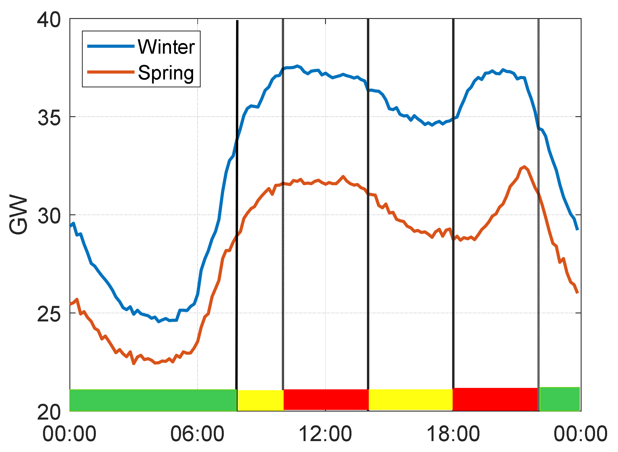
New tariffs in Spain became effective in June 2021. The new residential tariff 2.0TD is a three pricing period structure that replaces all the 2.x tariffs [44] (see Table 1). This regulatory change establishes higher prices on periods of higher consumption to promote demand shift management habits in the customers. In Figure 4, the demand profiles for the whole Spanish electrical system in representative days of winter and spring are plotted, and the selection of peak periods in accordance with the two periods of maximum electricity demand in the Spanish electrical system are clear.

2.2.4. Economic Balance

The economic balance was calculated on an hourly basis using the prices of electricity published by the Spanish TSO Red Eléctrica de España in its webpage ESIOS [43] and the energy balances were calculated with Equations (1) and (2). The economic savings S are composed of two parts: the cost of self-consumed PV-produced energy A (not imported from the grid), calculated according to Equation (6); and the value of the surplus energy (PV-produced and not self-consumed) compensated with the grid C .
A = i = 1 n E P V i E s r p l i   · P r r e t i b e i n g   i   t h e   i t h   h o u r   o f   t h e   m o n t h P r r e t i   t h e   r e t a i l   p r i c e   o f   e l e c t r i c i t y   o n   t h e   i t h   h o u r
The surplus compensation mechanism states that the surplus energy fed into the distribution grid is valuated at a price indexed to the wholesale market price (slightly lower), and that the final balance (the energy term in the monthly bill) cannot be negative. Thus, the value of compensated surplus energy can be expressed in Equation (7).
C = i = 1 n E s r p l i · P r s r p l i i = 1 n E i n i · P r r e t i E s r p l i · P r s r p l i 0 C = i = 1 n E i n i · P r r e t i     i = 1 n E i n i · P r r e t i E s r p l i · P r s r p l i < 0 b e i n g   P r s r p l i     t h e   p r i c e   o f s u r p l u s   e l e c t r i c i t y   o n   t h e   i t h   h o u r .
So, the monthly economic savings are:
S = A + C
And the monthly cost of the electricity taken from the grid
M = i = 1 n E i n i · P r r e t i
The electricity cost without PV would be the cost of the consumed energy valuated at retail price
B = i = 1 n E i · P r r e t i
The annual balances for the reference PVSCS and old and new tariffs are calculated and presented in Table 2. Due to the changes in tariffs in June 2021, the hourly prices for the new tariff 2.0TD before June 2021 and for the old tariff 20A after May 2021 were calculated accordingly to the tolls of both tariffs. For this consumer without PVSCS, the annual bill with the new tariff 2.0TD is almost equal to the former tariff 2.0A. Regarding the bill with PVSCS installed, the new tariff 2.0TD was 6.4% lower than the 2.0A, and the total savings were 12% higher for the new 2.0TD tariff over the 2.0A. These higher economic savings for the PV self-consumed electricity were due to the highest electricity prices from 10 a.m. to 2 p.m. in this new tariff, just in a period of high PV production.
These total savings are the cashflow that were then used for the calculation of the relevant economic indicators (TROI, NPV, IRR, LCOE) widely used in PVSCS financial analysis [45]. A linear degradation of PV production of 0.8% annually was assumed [46]. This translates to a reduction of 0.8% in the cashflow. The lifespan for the PVSCS is assumed to be 25 years, including the cost of a replacement of the inverter in the 13th year. Considering the sizes of residential PVSCS installations, the operation costs would be zero and the maintenance cost were estimated to be 1% of the value of the installation paid on a yearly basis, in line with published results [47]. The discount rate was selected as 1% based in the economic indicators for Spain and the Euro zone.
The study incorporates the time of return on investment (TROI) as the first economic measure. TROI is one of the most widely used methods for comparing the benefits of a program with the same costs per unit, per person or aggregated for the program as a whole. TROI was selected because it is a cost-benefit-oriented economic method [48]. Still, it is also used to calculate the return on investment (ROI), i.e., how much is produced by how much is invested. The cost of the systems under study is based in actual prices of this kind of installations.
An additional way of incorporating the economic feasibility study is to study the net present value (NPV) as a more robust measure of economic calculation. The NPV, expressed in Equation (11), represents the discounted value of all cash flows at the source at a discount rate that matches the cost of capital. The NPV values the unrealized cost of the investment project (i.e., the initial outlay) at a given point in time and the expected higher satisfaction in the future (i.e., the expected cash flows). It applied a process of choosing the current point in time as the point at which both the payout and the cash flows should be valued, so a discounting process was applied. To apply this discounting process, a discounted rate was incorporated, which is the opportunity cost of the project, known as the cost of capital.
N P V = I 0 + t = 1 n F t ( 1 + k ) t = I 0 + F 1 1 + k + F 2 ( 1 + k ) 2 + + F n ( 1 + k ) n
where
F t   are   the   cash   flows   in   each   period   t ;
I 0   is   the   initial   investment   at   t = 0 ;
n   is   the   number   of   periods ;
k   is   the   discount   rate   or   the   interest   rate   required   for   the   investment .
Another criterion used to make the study more robust was the so-called internal return ratio or IRR. It is defined as the discount rate that equals the NPV of the investment to 0, as shown in Equation (12). Its result is expressed as a percentage value. The IRR provides us with one of the most widespread measures of profitability as it provides a more intuitive idea of the adequacy to what is expected from an investment, as it is a value that can be easily compared with interest rates, which is one of the main components that determine the cost of capital in a given project.
N P V = I 0 + t = 1 n F t ( 1 + I R R ) t = 0
Finally, the levelized cost of electricity (LCOE) is a metric that informs about the cost of electricity independent of the technology used for generation. From the costs of the different installations, the LCOE was calculated following the procedure as exposed in [44] and expressed in Equation (13).
L C O E = t = 0 T C t / 1 + r t t = 0 T E t / 1 + r t
where   C t   are   the   cos ts ,   E t   i s   the   energy   produced ,   and   r   is   the   discount   rate .

2.2.5. Life Cycle Analysis

Photovoltaic technology does not produce CO2 emissions during its operation, but this technology presents several environmental impacts, mainly during manufacturing and disposal of the components. The life cycle analysis of the PVSCS was evaluated for the PV modules and the balance-of-system (inverter, cabling, structures, etc.). The net saving of emissions is calculated from Equation (14).
C a r b o n   B a l a n c e = E P V y · 1 N 1 0.008 n · L C E g r i d L C E P V S C
In addition, the greenhouse gas and energy payback time are calculated from Equations (15) and (16).
G P B T = L C E P V S C E P V y · L C E g r i d
E P B T = E P V + E B o S E P V y ·
where   E P V ,   E B o S   are   the   energy   needed   for   manufacturing   the   P V   modules and   the   balance of system .

2.3. Case Study #2: Industrial PVSCS

The second case under study is an industrial PVSCS for a meat-processing plant in Guijuelo (40°34′ N, 5°40′ W, province of Salamanca). The annual electricity consumption for the factory was 665 MWh before the expansion and was estimated to be more than 1000 MWh when the factory is fully operational, so the owners wanted to generate the most annual electricity as possible. As the new building was projected with a flat roof for easing the operation and maintenance of the PVSCS, several layouts for the PVSCS were analyzed.
The Canadian Solar CS3W-440MS PERC 440 W modules were proposed for installation, coupled with SolarEdge P950 power optimizers [49] and connected to 82.5-kW three-phase SolarEdge inverters [50]. During the design stage of this plant, several layouts were considered. The PVSYST simulations used the PVGIS database due the temperature data being more accurate for this location compared to the Meteonorm 7.3 database. The models for the PV modules, power optimizers, and the inverters were provided with version 7.1 of PVSYST. Modules and strings allocation and orientation in the simulations were as close as projected as is allowed by the software. The oversizing of DC PV power over inverter nominal power was small for the three options, because the SolarEdge 82.5 kW inverters were composed of three 27.5-kW units. The detailed electrical model option was not available for mixed orientations connected to one inverter. As there were few shadings, PV modules are half-cell type, and power optimizers were used, the linear shading option was selected for the simulations. The error for this shading option was about 3% for all configurations with an error less than 1% between them in the comparison.
The results from the simulations will be presented in Section 3 and there will be explained the selected and built layout, shown in Figure 5, together with preliminary results of the first year of operation.

3. Results

3.1. Residential PVSCS

The first step in the study is a preliminary energy analysis of the electricity consumption in the building and the electricity production of the original PVSCS, which will be achieved using heatmaps. Figure 6a represents the hourly consumption profile of the home. It can be observed that there are two usual patterns. In the summertime, the consumption is higher from 12 p.m. to 3 p.m. due to cooking and in the afternoon due to the use of air conditioning. The rest of the year is higher from 8 p.m. to 12 a.m. due to the use of the heat pump for heating. Exceptions are in spring, with low consumption all day, and, in some weeks in winter, the consumption is very high due to the colder weather. In Figure 6b, the PV production is represented and fits well with the peak consumption in summer.

3.1.1. Energy Analysis

As was explained in the previous section, the different alternative configurations for the PVSCS were simulated in PVSYST and compared with the real data obtained from the PVSCS. In Table 3, the size and specific yield for the original installation based on the measured data (first line) and for the simulated original installation and the alternative ones are shown. It can be seen that the difference between the simulation and the real measured data were less than 1% for the original configuration (simulated is worst). This is a fair result considering the natural variability of yearly irradiation and reported results for PVSYST simulations [37], so the original simulated configuration will be the reference for the analysis. The energy optimum configuration is 11% better than the original one. Regarding the alternative configurations placed on the façades, the results range from a 10% lesser yield for the configuration using canopies and a 30% lesser for the configurations with coplanar modules attached to the façades.
The energy balances are presented in Table 4. The PV production for the original configuration (both simulated and measured) and for the canopy and façade configuration are very close. Nevertheless, the simulated PV self-consumed energy differs from the 3.4 MWh vs. 3.0 MWh measurements. This can be explained due to different hourly profiles for the irradiance in the meteorological database used for the simulation and the real irradiance in the period under study. So, in the following, the comparison between the different alternatives will be made with the original simulated configuration. In this way, the effects of different meteorological data are cancelled because the same data are used for all configurations.
The canopy and the energy optimal configuration have similar PV production and self-consumption, bearing in mind that the canopy configuration has a PV power which has 20% more installation. The façade configuration has the lower PV production, which is 16% lower than the original simulated, but the self-consumed energy is only 2% lower.
Considering that these data are not clear enough, the effect of the PV orientations on the self-consumption variation. For a given consumption profile, the amount of self-consumed PV electricity depends mainly on two factors: the total amount of the PV production in a given period of time (daily, monthly, yearly) and its profile. For example, if a particular configuration produces less energy, it is easier to consume it in the building, improving the self-consumption degree.
The method used for distinguishing the effect of the different production profiles is as follows. For each configuration, the PV production profile was rescaled to match annual energy productions ranging from 5000 kWh to 15,000 kWh and the energy balances were calculated in each case, simulating the behavior of PV installations of different installed powers, usually denoted as “peak power”. Working in this way, it was possible to distinguish the effect of the different orientations on the self-consumption and self-sufficiency indexes. Figure 7 presents (a) the self-consumption and (b) the self-sufficiency degree (defined in Equations (3) and (4)). The result is that the alternative configurations provide a self-consumption index which is 4% better than the original and 2% better than self-sufficiency. This is a consequence of the flatter time profile of the PV production for the configurations based on modules coplanar with the façades and on canopies.

3.1.2. Economic Analysis

The hourly energy balances are valuated with the pricing data for the two tariffs, as detailed in Equations (6)–(10), and the annual PV profits are calculated for all configurations and annual productions. The results are shown in Figure 8 and can be seen that, for the same energy production, the most profitable configuration is the one with modules coplanar with the façades. This is due to the superior self-consumption of PV-produced electricity which is valuated at a higher price than the surplus energy exported to the distribution grid. It is also visible in Figure 8b that the annual profit rises linearly with the PV production up to 9 MWh and beyond this annual production. The profit then increases at a slower pace. This is due to the Spanish simplified compensation expressed in Equation (7) which establishes that, during the one-month billing period, the energy term cannot be negative. In fact, for higher PV productions, in some months, it is possible for the value of the energy exported to the grid to be higher than the consumption, despite the lower price of the exported energy, thus reducing the profits. In addition, by comparing the profits for the two tariffs, the new tariff displays a profit of approximately EUR 100 higher than the older one for all configurations and sizes.
The annual profits calculated are used as the cashflow for the economic analysis. The other input are the costs of the installations. The costs were estimated as follows: 1.55 EUR/W for PV powers lower than 4 kW, 1 EUR/W for PV powers higher than 8 kW, and a linear variation of costs between these powers. This pricing scheme is supported on the information of PV installers, and it is representative of the Spanish PV residential market in the year 2021. We applied a cost increase of 11% for the configuration based on façades, 12.5% for the mixed one, and 14% for the canopies. Figure 9 presents the results for the net present value (a,d), the internal rate of return (b,e), and the time of return of investment (c,f). These results are plotted versus the annual PV production (a–c) and versus the installed PV power (d–f). The economic indicators are favorable in all cases, i.e., the optimal case is the best economic performer and the façades are the worst. The best maximum NPV is for the optimal case with EUR 12,271 and 8.1 kW installed at a cost of EUR 8116. The lowest NPV is the highest at EUR 7616, and is almost flat for a range of powers between 8 kW and 11 kW. The IRR is also very favorable, always over 7%. The best performer is the optimal, between 14% and 17% and the worst the façades, between 6.9% and 10.8%. The optimal PV power is around 8 kW in all cases. The time of return of investment is the smallest for PV power of 8 kW in all cases and ranges from 6.3 years for the optimal case to 8.6 years for the façades.
Finally, the levelized cost of electricity is calculated according with Equation (13) and is shown in Figure 10a,b. For PV powers under 8 kW, the LCOE reach maximum values between 6.3 EUR/kWh and 10.3 EUR/kWh. and the minimum values are between 4.0 EUR/kWh and 7.0 EUR/kWh. All these minimum values are well below current retail electricity prices in Spain.

3.1.3. Life Cycle Assessment

The carbon balance of the PVSCS is calculated according to Equation (14) and the greenhouse gas and the energy payback according to Equations (15) and (16). The emissions factor for the Spanish electricity production is 0.19   t C O 2 / M W h [51], and the emissions for a Chinese-made PV module of 811   k g   C O 2 e q / k W p [52] and 519   k g   C O 2 e q / k W p for the balance-of-system (BoS) [53]. The results are shown in Table 5 and show the good footprint of all the configurations. For the more conventional installations on the roof, the greenhouse gas payback time (GGPBT) is between 4.1 and 4.4 years, and the energy payback time (EPBT) between 1.6 and 1.8 years. For the installation on façades, the GGPBT is between 5.1 and 6.5 years and the EPBT between 2.0 and 2.5 years. Considering the projected lifetime of 25 years, all these installations will produce between 9 and 14 times the energy invested in their deployment (EROI, energy return on investment).

3.2. Industrial PVSCS

The annual electricity consumption for the factory was 665 MWh before the expansion and was estimated to be of 1000 MWh for when the factory is fully operational, so the owners wanted to generate the most electricity as possible. As the new building was projected with a flat roof for easing the operation and maintenance of the PVSCS, several layouts for the PVSCS were analyzed. The reference and the first option considered was the optimal energy producing orientation (South, 35° inclination). The limitation for this option is the wide separation between rows mandatory for avoiding mutual shading due to the high angle of inclination, causing a poor occupancy of the available area in the roof. In order to accommodate the maximum number of PV modules, a lower inclination of 15° with South orientation was selected and two other orientations were analyzed: east–west and two perpendicular orientations aligned with the principal axes of the building. It is important to note that, due to the high winds present in the winter, modules should be placed in landscape orientation and with the lowest possible inclination.
The four layouts considered were simulated in PVSYST using the same PV modules, power optimizers, inverters, meteorological database, and simulation options. The results are presented in Table 6 and all the orientations have acceptable specific yields, ranging between 1495 kWh/kWp and 1729 kWh/kWp. The main goal of this installation was to reach the maximum annual energy production, and the four layouts in two groups of similar productions (the lower production group for the optimal energy-producing and the east–west layout) were discarded.
The south orientation and the two orientations (both 15° inclination) exhibit higher annual production, with better specific yield and less production compared to the south one. Finally, the south orientation was discarded because of three reasons: lower annual energy production, poor accessibility to all parts of the installation, and sharper PV production profile.
The Spanish regulation allows a fast-permitting process for PVSCS without surplus for installations of nominal power above 100 kW in most regions, for example in Castille and León [54]. For installations with a surplus above 100 kW, it is mandatory to obtain permits for grid connection [55] so there are several permitting stages that would delay the process both before and after building the PVSCS. In addition, the biggest portion of energy consumption is the cooling inherent to the meat processing; thus, the energy consumption in summer is double that in winter. In this way, the first option (south orientation) was discarded because it yields a sharper maximum at solar noon, so there is the risk of frequently producing more electricity than the consumption, so the inverters would curtail the production. For the two-orientation layout, the daily production presents a flatter peak around midday and produces electricity for a longer time in spring and summer, being reflected in a higher daily production.
In Figure 11, the hourly production for two clear-sky days with extreme solar trajectories is presented. Figure 11a corresponds to a day near winter solstice and Figure 11b to a the summer solstice. For a better view of the effect of orientation (azimuth and inclination), the data from the four configurations are rescaled to 169 kW. It can be seen that, due to the low inclination of the modules, the variation between the South (15° inclination) orientation layout and the 2-orientation layout is low. However, in summer, the 2-orientation production profile is more rounded, with a lower peak and higher production at sunrise and sunset. The east–west configuration has a marginally better behavior in summer, but it is poor in winter. On the contrary, the energy-optimal orientation (South, 35° inclination) presents a better performance in winter but a worse one in summer with a sharper profile, with the lowest production in the morning and in the evening. It is important to reiterate that the installed PV power for the optimal south orientation and the east–west layouts is significantly lower than for the South (15°) and the two-orientation layouts.
Finally, the two-orientation layout was selected. This installation has a peak power of 169 kW. It comprises 386 Canadian Solar CS3W-440MS PERC 440 W modules with 193 SolarEdge P950 power optimizers [49] and two 82.5 kW three-phase SolarEdge inverters [50] for a maximum nominal power of 165 kW, as shown in Figure 5. The modules are distributed in 11 strings of 16 power optimizers and one of 17 power optimizers (32 or 34 modules/string). The estimated yearly production is 270 MWh with a specific yield of 1597 kWh/kWp and a performance ratio of 82%.
The behavior of the built PVSCS on one representative day is presented in Figure 12. As can be seen, the energy consumption decreases at lunchtime, between 14:00 and 16:00. This can make the electricity consumption from the grid too low, so the inverters curtail the production. According to the Spanish regulation [21], if the PVSCS is connected under the category without surplus, grid feeding is not allowed in any of the three electricity phases, as can be seen in the production curtailed around 16:00. So, if the electrical loads into the factory are not well-balanced, it could result in higher PV production losses. This fact is important in favor of PVSCS layouts that yield the energy with flatter and longer production profiles.
This PVSCS is in operation since October 2020, and there are data for the PV production for a year, but the factory did not go fully operational until 2021, so the analysis cannot be as complete as for the residential example. Figure 13 shows the heatmaps for the hourly consumed energy (Figure 13a), PV-produced energy (Figure 13b), and imported energy from the grid (Figure 13c). A good fit between the factory peak load before noon and the PV production can also be appreciated. Furthermore, in Figure 13c, a near-zero consumption period can be seen due to the PVSCS production. It is important to note the reduction in the maximum hourly energy demanded from the grid in periods of high prices of electricity.

4. Discussion

The use of PV orientations non-optimal for energy generation was presented in residential and industrial cases of study. For the residential case, it is found that the economic yield for the discussed orientations is better than its energy yield. One reason is that, by using several orientations, the energy production spreads more uniformly during the daytime, increasing the self-consumption share of PV-produced electricity. The other reason is found in the variable prices for the retail electricity and the surplus electricity fed into the distribution grid. With the maturity of the PV sector, the actual net-billing schemes, such as the current one in Spain, are more appropriate than net-metering policies since the surplus price is indexed to the wholesale electricity market, thus signaling the periods when distributed generation is more valuable [56]. The use of these non-optimal orientations can reduce the electricity interchanged with the grid, especially the energy fed, resulting in a reduction in the energy stress on the grid [57]. Another benefit can be a more stable production for configurations using façades, which can provide a better match with the consumption profile during the year.
The introduction of residential tariffs with higher prices in periods of high electricity consumption will add an additional profit to the Southeast orientations, which produce most electricity in the hours before noon, just within one of the two peak tariff periods. From the data shown in Figure 8, the increase in profits over the current one period tariff ranges between 8% and 16% for PV installations of annual productions from 5 MWh to 15 MWh.
For the industrial case, in addition to the considerations discussed for the residential scenario, there are additional factors to take into account. The use of alternative orientations can facilitate larger PVSCS, reduced curtailment of PV production or energy fed into the distribution grid, and simplified installation and maintenance. Furthermore, it is possible to optimize the periods of energy generation to suit the load patterns of the site. The use of PV reduces the maximum power demanded from the grid, in particular, the analysis of the period of available data shows an important reduction in power surpasses. In Spanish industrial tariffs, a surpass is defined as the power demanded in a quarter-hour period exceeds the contracted power. For this industry, the contracted power is 180 kW and, in the first year of operation, there are 1924 quarters with consumption over 180 kW, with a maximum demanded power of 325.89 kW. For the energy taken from the grid, there are 761 quarters with demanded power over 180 kW and with a maximum power demanded from the grid of 293.06 kW. These figures mean that the use of PV roughly decreases the surpasses by 60% and the maximum power exceeded decreases a 23%, reducing maximum demand penalties and providing additional economic savings. The results are in line with the findings in [58], specifically for the small influence of the azimuth angle and the noticeable gains in annual energy production which reduce the tilt angle.
To realize the potential of alternative orientations, it is important to stress the necessity of implementing complementary demand side strategies. For example, in Figure 4, it is clear that the use of air conditioning during the night in summer can be shifted to the hours when PV production is high using self-produced PV electricity, therefore providing greater economic benefit.
From a wider perspective, the use of these orientations can provide an important increase in the suitable area for PV, beyond roofs [59,60]. Traditionally, installations of PV in locations other than roofs are perceived as inefficient or uneconomic and are reserved for emblematic or flagship buildings. The present study shows that, even when the energy performance is lower than traditional orientations, the economic performance is not so far from them. Considering that PV modules can replace building materials, the overall economic balance can be positive. In addition, the use of PV as shading elements in canopies can be used by architects to improve the user’s comfort and the energy performance of the building by reducing cooling while increasing the energy production. These facts are relevant to the BIPV concept and can help to expand this sector.
As solar PV is on the verge of its massive deployment in edifications, it is important to pay attention to the economic viability as well as its ecological and environmental footprint. A basic life cycle assessment study was performed for the residential case and the carbon balance, greenhouse gas, and energy payback times are good for all the configurations under study and in line with other studies [45,53]. It is important to note that the analysis was carried out with consideration of the manufacturing of the PV components in a country with high emissions in electricity production (China) and the deployment in a country (Spain), with emissions as low as 1 / 4 compared to that of the manufacturer.
Complementarily, these results help us to demystify the general rules of thumb of photovoltaic installations, such as: “In the northern hemisphere, the solar panels have to be oriented towards the South” and “For maximum annual energy availability, a surface slope equal to the latitude is best” [61]. More precisely, in an extensive numerical study [62], the optimal fixed tilt and azimuth angles are calculated for the continental USA and it is found that “The optimum tilt was never greater than latitude tilt, but up to 10° less than latitude tilt”. In this reference, is also pointed that, if variable electricity prices are considered, these angles can vary. Moreover, as stated in [63], “there is a false perception among building professionals that solar modules should be installed on ideally oriented and tilted surfaces”. The performance of systems with non-optimal orientations allows further flexibility in the installation of PVSCS in residences and industrial buildings. This is achieved without aesthetically distorting the structure and obtaining an acceptable economic benefit with an economic yield that varies only slightly compared to installations with optimal orientations.
Future directions of this work will include a detailed techno-economic analysis of the industrial PVSCS with full-year data of both PV production and factory electricity consumption; systematic research of different orientations for representative, residential, commercial, and industrial users; and the development of a methodology for optimal design of PV installations in accordance with hourly-variable electricity prices and consumption patterns.

5. Conclusions

The results presented in this work show that the most common option for the orientation of PV modules (optimal for annual module production) is not always the most favorable for self-consumption installations. For this purpose, two specific cases have been studied of PVSCS in residential and industrial buildings.
In the case of PVSCS in residential buildings, the PVSCS located in a building in the Madrid metropolitan area was studied and, using these initial annual data, the results obtained under other PV layouts were simulated; these new layouts used canopies and on façades. With these values, calculations were made to obtain the energy and economic balance of each configuration, concluding that PVSCS installed in orientations other than the traditional optimum for energy production are a viable option. This is largely since the new residential tariffs represent an increase of up to 12% in profit over the previous tariffs. This advantage is coupled with the advantage offered by using other architectural surfaces than the roof, which are not in optimal orientations; this means that a higher power PVSCS can be built and that a higher annual electricity production will be realized. The method used for obtaining a proper comparison between installations of different specific yields was to rescale the PV production to fixed values in a range of annual consumptions representative of Spanish residential sector. The analysis proves that the economic performance of these orientations is acceptable under the self-consumption net billing scheme in force in Spain.
  • The specific yield ranges from 1097 kWh/kWp for the modules on façades to 1375 kWh/kWp for the canopies and 1560 kWh/kWp for the original configuration, which compares with 1725 kWh/kWp of the energy optimal.
  • The self-sufficiency index improves up to a 2% over the optimal energy.
  • The internal rate of return is highest for a PV power of 8 kWp for all layouts and ranges from 10% to 17%.
  • The time of return of investment is lowest for a PV power of 8 kWp and ranges from 6.5 to 9 years.
An additional advantage for these orientations is found in the new residential tariffs, resulting in an increase up to 12% in profit over previous tariffs. The new period of highest prices which “peak” before noon can be used in orientations with maximum production in this period. There is also a fair economic performance for these orientations, despite the higher cost assumed in this study for the modules placed on canopies and on the façades.
The environmental indicators are good for the alternative installations in non-optimal orientations:
  • The maximum greenhouse gas payback time is 6.4 years for the installation of modules coplanar with the façades.
  • The average energy payback time rises to 2.0–2.1 years for modules placed on façades from 1.6–1.8 years for modules on the roof.
The data from the industrial PVSCS case study suggest that non-optimal PV orientations can present an advantage over traditional south-facing orientations with inclination optimal for yearly energy production. The main advantages found can be summarized as follows:
  • Higher installed power due to more efficient use of available space in roofs, resulting in higher energy production in the available space. The benefit identified in the case study was a 72% higher peak power and a 59% increase in energy production.
  • Improved economic yield by adaptation to variable electricity tariffs and load patterns of industry using different orientations.
  • Reduced curtailment of PV production or energy fed into the distribution grid due to the flattened production profile.
  • Higher potential for reducing peaks of consumption due to the extended period of PV production. The reduction in the number of powers surpasses 69% and the maximum power exceeded is reduced to 45% in this case study.
  • A more orderly PV layout; easier installation, operation, and maintenance; and improved overall safety for workers.
With the current outlook of an increased deployment of zero-marginal-cost generation sources, such as PV, wholesale market electricity prices are expected to decline after noon, when consumption is lower. Meanwhile, retail prices will remain high during peak periods of consumption and, therefore, the use of non-optimal orientations can be highly beneficial from an economic point of view.

Author Contributions

Conceptualization, E.S. and Á.O.; methodology, E.S. and Á.O.; software, E.S.; investigation, E.S., Á.O. and J.P.-D.; resources, E.S. and A.S.; data curation, E.S.; writing—original draft preparation, E.S., Á.O. and J.P.-D.; writing—review and editing, E.S., Á.O., A.S., R.G.O. and J.P.-D.; visualization, E.S.; supervision, R.G.O.; project administration, E.S. and R.G.O.; funding acquisition, R.G.O. All authors have read and agreed to the published version of the manuscript.

Funding

This research was funded by “Fundación Memoria de D. Samuel Solórzano Barruso”, grant number FS/21-2019.

Data Availability Statement

Restrictions apply to the availability of these data.

Acknowledgments

The authors wish to thank Roberto Vicente Babiano for sharing the data from his home PVSCS, Marcial Castro S.L. for sharing the data from its new factory PVSCS, and Manuel Hernández and Grupo JC for the drone photograph.

Conflicts of Interest

One of the authors (A.S.) redacted the engineering project and was responsible of the works direction for the PVSCS in the industrial plant. E.S. collaborate in this project with the analysis of the different configurations and the PV design and calculations for the final layout. There is no other conflict of interest.

Abbreviations

BAPVBuilding-applied photovoltaics
BIPVBuilding-integrated photovoltaics
BIPV/TBuilding-integrated photovoltaic thermal
BoSBalance of System
CNMCNational commission for markets and competition
FiTFeed-In-Tariff
ICPSwitch for power control
IRRInternal return rate
LCOELevelized cost of energy
NPVNet present value
NZEBNearly-zero energy buildings
PERCPassivated emitter rear contacts
PVPhotovoltaic
PVGISPhotovoltaic geographical information system
PVPCVoluntary price for small consumer
PVSCSPhotovoltaic self-consumption system
REERed Eléctrica de España
ROIReturn on investment
SCDSelf-consumption degree
SSDSelf-sufficiency degree
TROITime of return of investment
TSOTransmission system operator
VATValue-added tax

References

  1. Shahsavari, A.; Akbari, M. Potential of solar energy in developing countries for reducing energy-related emissions. Renew. Sustain. Energy Rev. 2018, 90, 275–291. [Google Scholar] [CrossRef]
  2. Sharif, A.; Meo, M.S.; Chowdhury, M.A.F.; Sohag, K. Role of solar energy in reducing ecological footprints: An empirical analysis. J. Clean. Prod. 2021, 292, 126028. [Google Scholar] [CrossRef]
  3. Kosorić, V.; Huang, H.; Tablada, A.; Lau, S.K.; Tan, H.T.W. Survey on the social acceptance of the productive façade concept integrating photovoltaic and farming systems in high-rise public housing blocks in Singapore. Renew. Sustain. Energy Rev. 2019, 111, 197–214. [Google Scholar] [CrossRef]
  4. Strazzera, E.; Statzu, V. Fostering photovoltaic technologies in Mediterranean cities: Consumers’ demand and social acceptance. Renew. Energy 2017, 102, 361–371. [Google Scholar] [CrossRef]
  5. IEA. Global Energy Review 2021; International Energy Agency: Paris, France, 2021. [Google Scholar]
  6. Fthenakis, V.; Mason, J.E.; Zweibel, K. The technical, geographical, and economic feasibility for solar energy to supply the energy needs of the US. Energy Policy 2009, 37, 387–399. [Google Scholar] [CrossRef]
  7. DNV GL. Energy Transition Outlook 2018 Power Supply and Use; DNV: Bærum, Norway, 2018. [Google Scholar]
  8. Green, M.A. Third generation photovoltaics: Solar cells for 2020 and beyond. Phys. E Low-Dimens. Syst. Nanostruct. 2002, 14, 65–70. [Google Scholar] [CrossRef]
  9. Singh, G.K. Solar power generation by PV (photovoltaic) technology: A review. Energy 2013, 53, 1–13. [Google Scholar] [CrossRef]
  10. SolarPower Europe. EU Market Outlook for Solar Power 2019–2023—SolarPower Europe. Available online: https://www.solarpowereurope.org/eu-market-outlook-for-solar-power-2019-2023/ (accessed on 12 April 2021).
  11. SolarPower Europe. EU Solar Boom: Over 100% Solar Market Increase in 2019—SolarPower Europe. Available online: https://www.solarpowereurope.org/eu-solar-boom-over-100-solar-market-increase-in-2019/ (accessed on 12 April 2021).
  12. UNEF. Informe Anual Unef 2021; Unión Española Fotovoltaica: Madrid, Spain, 2021. [Google Scholar]
  13. de España, G. PNIEC 2021–2030; Ministerio Para la Transición Ecológica y el Reto Demográfico: Madrid, Spain, 2021. [Google Scholar]
  14. Agathokleous, R.A.; Kalogirou, S.A. Status, barriers and perspectives of building integrated photovoltaic systems. Energy 2020, 191, 116471. [Google Scholar] [CrossRef]
  15. Fath, K.; Stengel, J.; Sprenger, W.; Wilson, H.R.; Schultmann, F.; Kuhn, T.E. A method for predicting the economic potential of (building-integrated) photovoltaics in urban areas based on hourly Radiance simulations. Sol. Energy 2015, 116, 357–370. [Google Scholar] [CrossRef]
  16. Shukla, A.K.; Sudhakar, K.; Baredar, P. A comprehensive review on design of building integrated photovoltaic system. Energy Build. 2016, 128, 99–110. [Google Scholar] [CrossRef]
  17. Energy Performance of Buildings Directive|Energy. Available online: https://ec.europa.eu/energy/topics/energy-efficiency/energy-efficient-buildings/energy-performance-buildings-directive_en (accessed on 23 November 2020).
  18. Dávi, G.A.; Caamaño-Martín, E.; Rüther, R.; Solano, J. Energy performance evaluation of a net plus-energy residential building with grid-connected photovoltaic system in Brazil. Energy Build. 2016, 120, 19–29. [Google Scholar] [CrossRef] [Green Version]
  19. Briano, J.I.; Fondo Roca, C.; Fasolino, J.D. Pv Grid Parity Monitor: Madrid, Spain; 2016. Available online: https://www.creara.es/informe/pv-grid-parity-monitor-commercial-sector-3rd-issue?lang=en (accessed on 8 October 2021).
  20. López Prol, J.; Steininger, K.W. Photovoltaic self-consumption is now profitable in Spain: Effects of the new regulation on prosumers’ internal rate of return. Energy Policy 2020, 146, 111793. [Google Scholar] [CrossRef]
  21. Gobierno de España; Mincotur. Real Decreto 244/2019, de 5 de Abril, Por el Que se Regulan Las Condiciones Administrativas, Técnicas y Económicas Del Autoconsumo de Energía Eléctrica; Boletín Oficial del Estado: Madrid, Spain, 2019; p. 35674. [Google Scholar]
  22. Gobierno de España. Real Decreto-Ley 15/2018, de 5 de Octubre, de Medidas Urgentes Para la Transición Energética y la Protección de los Consumidores; Boletín Oficial del Estado: Madrid, Spain, 2018; p. 97430. [Google Scholar]
  23. Ordóñez Mendieta, Á.J.; Sánchez Hernández, E. Analysis of PV Self-Consumption in Educational and Office Buildings in Spain. Sustainability 2021, 13, 1662. [Google Scholar] [CrossRef]
  24. Sánchez, E.; Izard, J. Performance of photovoltaics in non-optimal orientations: An experimental study. Energy Build. 2015, 87, 211–219. [Google Scholar] [CrossRef]
  25. Evola, G.; Margani, G. Renovation of apartment blocks with BIPV: Energy and economic evaluation in temperate climate. Energy Build. 2016, 130, 794–810. [Google Scholar] [CrossRef]
  26. Fogl, M.; Moudrý, V. Influence of vegetation canopies on solar potential in urban environments. Appl. Geogr. 2016, 66, 73–80. [Google Scholar] [CrossRef]
  27. Haysom, J.E.; Hinzer, K.; Wright, D. Impact of electricity tariffs on optimal orientation of photovoltaic modules. Prog. Photovolt. Res. Appl. 2016, 24, 253–260. [Google Scholar] [CrossRef]
  28. PVSYST Photovoltaic Software. Available online: https://www.pvsyst.com/ (accessed on 28 September 2021).
  29. Cebecauer, T.; Skoczek, A.; Šúri, M. The effect of solar radiation data types on calculation of tilted and suntracking solar radiation. In Proceedings of the 26th European Photovoltaic Solar Energy Conference and Exhibition, Hamburg, Germany, 5–9 September 2011; pp. 4297–4302. [Google Scholar]
  30. Mermoud, A.; Lejeune, T. Performance Assessment of a Simulation Model for PV Modules of Any Available Technology. In Proceedings of the 25th European Photovoltaic Solar Energy Conference and Exhibition, Valencia, Spain, 5–9 September 2010; pp. 6–10. [Google Scholar]
  31. Schwingshackl, C.; Petitta, M.; Wagner, J.E.; Belluardo, G.; Moser, D.; Castelli, M.; Zebisch, M.; Tetzlaff, A. Wind effect on PV module temperature: Analysis of different techniques for an accurate estimation. Energy Procedia 2013, 40, 77–86. [Google Scholar] [CrossRef] [Green Version]
  32. Urraca, R.; Gracia-Amillo, A.M.; Koubli, E.; Huld, T.; Trentmann, J.; Riihelä, A.; Lindfors, A.V.; Palmer, D.; Gottschalg, R.; Antonanzas-Torres, F. Extensive validation of CM SAF surface radiation products over Europe. Remote Sens. Environ. 2017, 199, 171–186. [Google Scholar] [CrossRef] [PubMed] [Green Version]
  33. Meteonorm. Handbook Part II (7): Theory Global Meteorological Database Version 7 Software and Data for Engineers, Planers and Education; Meteotest AG: Bern, Switzerland, 2020. [Google Scholar]
  34. ETH Zurich Global Energy Balance Archive Data. Available online: https://geba.ethz.ch/ (accessed on 8 October 2021).
  35. EU JRC PVGIS-SARAH. Available online: https://ec.europa.eu/jrc/en/PVGIS/downloads/SARAH (accessed on 8 October 2021).
  36. Erbs, D.G.; Klein, S.A.; Duffie, J.A. Estimation of the diffuse radiation fraction for hourly, daily and monthly-average global radiation. Sol. Energy 1982, 28, 293–302. [Google Scholar] [CrossRef]
  37. Lee, G.R.; Frearson, L.R.P. An assessment of photovoltaic modelling software using real world performance data. In Proceedings of the 26th European Photovoltaic Solar Energy Conference and Exhibition, Hamburg, Germany, 5–9 September 2011; pp. 4339–4343. [Google Scholar]
  38. Google. Google Earth. Available online: https://earth.google.com/web/ (accessed on 28 September 2021).
  39. Muntwyler, U.; Schärf, P.; Münger, M.; Joss, D.; Hauser, M.; Heiniger, T. Comparison of PV evaluation programs based on the long-term PV-measurement campaign of the Berne University of Applied Sciences. In Proceedings of the 27th European Photovoltaic Solar Energy Conference and Exhibition, Frankfurt, Germany, 24–28 September 2012; pp. 4158–4160. [Google Scholar] [CrossRef]
  40. Wright, A.; Firth, S. The nature of domestic electricity-loads and effects of time averaging on statistics and on-site generation calculations. Appl. Energy 2007, 84, 389–403. [Google Scholar] [CrossRef] [Green Version]
  41. Cao, S.; Sirén, K. Impact of simulation time-resolution on the matching of PV production and household electric demand. Appl. Energy 2014, 128, 192–208. [Google Scholar] [CrossRef]
  42. Luthander, R.; Widén, J.; Nilsson, D.; Palm, J. Photovoltaic self-consumption in buildings: A review. Appl. Energy 2015, 142, 80–94. [Google Scholar] [CrossRef] [Green Version]
  43. Red Eléctrica de España (REE) Esios—Autoconsumo. Available online: https://www.esios.ree.es/es/analisis/1739?vis=1&start_date=16-03-2021T00%3A00&end_date=16-03-2021T23%3A00&compare_start_date=15-03-2021T00%3A00&groupby=hour&compare_indicators=1013,1014,1015 (accessed on 3 December 2020).
  44. Comisión Nacional de los Mercados y la Competencia. Memoria Justificativa de la Circular de la Comisión Nacional de los Mercados y la Competencia por la que se Establece la Metodología Para el Cálculo de los Peajes de Transporte y Distribución de Electricidad; CNMC: Madrid, Spain, 2020. [Google Scholar]
  45. Castilho, C.D.S.; Torres, J.P.N.; Fernandes, C.A.F.; Lameirinhas, R.A.M. Study on the implementation of a solar photovoltaic system with self-consumption in an educational building. Energies 2021, 14, 2214. [Google Scholar] [CrossRef]
  46. Jordan, D.C.; Kurtz, S.R.; VanSant, K.; Newmiller, J. Compendium of photovoltaic degradation rates. Prog. Photovolt. Res. Appl. 2016, 24, 978–989. [Google Scholar] [CrossRef]
  47. Steffen, B.; Beuse, M.; Tautorat, P.; Schmidt, T.S. Experience curves for operations and maintenance costs of renewable energy technologies. Joule 2020, 4, 359–375. [Google Scholar] [CrossRef]
  48. Catherine, C.; Rosenzweig, W.; Long, D.; Olsen, S. Double Bottom Line Project Report: Assessing Social Impact in Double Bottom Line Project Report: Assessing Social Impact in Double Bottom Line Ventures; Center for Responsible Business eScholarship Publishing: Berkeley, CA, USA, 2004; Available online: https://escholarship.org/uc/item/80n4f1mf (accessed on 15 October 2021).
  49. SolarEdge Technologies Ltd. SolarEdge Power Optimizers. Available online: https://www.solaredge.com/es/products/power-optimizer#/ (accessed on 27 September 2021).
  50. SolarEdge Technologies Ltd. SolarEdge Inverters. Available online: https://www.solaredge.com/es/products/pv-inverters/synergy-inverter#/ (accessed on 27 September 2021).
  51. Red Electrica de España. Emisiones de CO2 Asociadas a la Generación de Electricidad en España; Red Electrica de España: Alcobendas, Spain, 2020; Volume 2. [Google Scholar]
  52. Müller, A.; Friedrich, L.; Reichel, C.; Herceg, S.; Mittag, M.; Neuhaus, D.H. A comparative life cycle assessment of silicon PV modules: Impact of module design, manufacturing location and inventory. Sol. Energy Mater. Sol. Cells 2021, 230, 111277. [Google Scholar] [CrossRef]
  53. Fraunhofer ISE. Photovoltaics Report 2021; Fraunhofer Institute for Solar Energy Systems: Freiburg im Breisgau, Germany, 2021. [Google Scholar]
  54. Comunidad de Castilla y León. Decreto-Ley 4/2020, de 18 de Junio, de Impulso y Simplificación de la Actividad Administrativa Para el Fomento de la Reactivación Productiva en Castilla y León; Boletín Oficial de Castilla y León: Valladolid, Spain, 2020; p. 18492. [Google Scholar]
  55. de España, G. Real Decreto 1183/2020, de 29 de diciembre, de acceso y conexión a las redes de transporte y distribución de energía eléctrica. Boletín Of. Del Estado 2019, 2014, 18987–19106. [Google Scholar]
  56. Brown, P.R.; O’Sullivan, F.M. Shaping photovoltaic array output to align with changing wholesale electricity price profiles. Appl. Energy 2019, 256, 113734. [Google Scholar] [CrossRef]
  57. Thebault, M.; Gaillard, L. Optimization of the integration of photovoltaic systems on buildings for self-consumption—Case study in France. City Environ. Interact. 2021, 10, 100057. [Google Scholar] [CrossRef]
  58. Barbón, A.; Bayón-Cueli, C.; Bayón, L.; Rodríguez-Suanzes, C. Analysis of the tilt and azimuth angles of photovoltaic systems in non-ideal positions for urban applications. Appl. Energy 2021, 305, 117802. [Google Scholar] [CrossRef]
  59. Redweik, P.; Catita, C.; Brito, M. Solar energy potential on roofs and facades in an urban landscape. Sol. Energy 2013, 97, 332–341. [Google Scholar] [CrossRef]
  60. Brito, M.C.; Freitas, S.; Guimarães, S.; Catita, C.; Redweik, P. The importance of facades for the solar PV potential of a Mediterranean city using LiDAR data. Renew. Energy 2017, 111, 85–94. [Google Scholar] [CrossRef]
  61. Duffie (Deceased), J.A.; Beckman, W.A.; Blair, N. Available Solar Radiation. In Solar Engineering of Thermal Processes, Photovoltaics and Wind; John Wiley & Sons: Hoboken, NJ, USA, 2020; pp. 45–140. [Google Scholar]
  62. Lave, M.; Kleissl, J. Optimum fixed orientations and benefits of tracking for capturing solar radiation in the continental United States. Renew. Energy 2011, 36, 1145–1152. [Google Scholar] [CrossRef] [Green Version]
  63. Portolan dos Santos, Í.; Rüther, R. Limitations in solar module azimuth and tilt angles in building integrated photovoltaics at low latitude tropical sites in Brazil. Renew. Energy 2014, 63, 116–124. [Google Scholar] [CrossRef]
Figure 1. Environmental variables in PVSYST: irradiances (global horizontal and in plane of array) and temperatures (ambient and array). Note that the array temperature is not calculated when the irradiance is null.
Applsci 11 09954 g001
Figure 2. Residential building under study before PV installation. (a) Satellite image (Google Earth) (b) Floorplan with basic dimensions and orientation.
Applsci 11 09954 g002
Figure 3. Residential PVSCS PVSYST models (a) Original layout (b) Design using canopies (c) Design using modules attached to the façade.
Applsci 11 09954 g003
Figure 4. Load profile of Spanish electrical system on representative days (21 January 2021, 21 April 2021). The different pricing periods in tariff 2.0TD are highlighted, with the peak price periods correlated with daily maximum electricity demand periods.
Applsci 11 09954 g004
Figure 5. Industrial PVSCS (a) PVSYST model, view from the South. (b) Photograph of the plant.
Applsci 11 09954 g005
Figure 6. Heatmaps of measured hourly energy consumption (a) and PV production (b) for the period under study.
Applsci 11 09954 g006
Figure 7. Self-consumption (a) and Self-sufficiency (b) degree vs. PV production relative to the consumption for the simulated configurations.
Applsci 11 09954 g007
Figure 8. Economic profit for older and new electricity tariffs in Spain: (a) Annual profit for older tariff 2.0A; (b) Annual profit for the new tariff 2.0TD. Taxes of 5.11% of electricity and 21% VAT are included in the calculations.
Applsci 11 09954 g008
Figure 9. Economic balance. (a) Net present value vs. annual PV production; (b) internal rate of return vs. annual PV production; (c) time of return of investment vs. PV annual PV production; (d) net present value vs. PV installed power; (e) internal rate of return vs. PV installed power; (f) time of return of investment vs. PV installed power.
Applsci 11 09954 g009aApplsci 11 09954 g009b
Figure 10. Levelized cost of electricity for all configurations. (a) LCOE vs. annual PV production; (b) LCOE vs. PV installed power.
Applsci 11 09954 g010
Figure 11. PV production of the different configurations rescaled to the same rated power for industrial PVSCS on clear-sky days with extreme solar trajectories. (a) Winter solstice, (b) Summer solstice.
Applsci 11 09954 g011
Figure 12. Screenshot of the monitoring portal showing the electricity consumption and production on one spring day (18 May 2021). The figure shows the 15-min average power in Watts for the consumption and PV production.
Applsci 11 09954 g012
Figure 13. Heatmaps of hourly values for the industrial PVSCS (a) Electricity consumption (b) PV production (c) Energy imported from the grid.
Applsci 11 09954 g013
Table 1. Hourly distribution and comparison with horizontal solar irradiation for tariff 2.0.
Hour123456789101112131415161718192021222324
Winter Solstice irradiation (Wh/m2) 164294119300422314186928
2.0A“FLAT”
2.0DHA“VALLEY”“PEAK”
2.0VE“VALLEY”“PEAK”
Equinox irradiation (Wh/m2) 137527247263976183183676163347527275
NEW 2.0TD 2“VALLEY 2.0” “PEAK 2.0”“FLAT 2.0”“PEAK 2.0”
Summer Solstice irradiation (Wh/m2) 1125308503681608947103174458390067842233615314
1 Data corresponding to Madrid. Source AEMET. 2 “Valley” on weekends and public holidays. Red: Peak price rate (highest price). Yellow: Flat price rate (intermediate price). Green: Valley price rate (lower price).
Table 2. Economic performance of the PVSCS for a full year (August 2020 to July 2021) comparing the former tariff 2.0A and with the new 2.0TD tariff. Taxes are included.
Tariff M
Imported
A
Self-Cons.
C
Surplus
Bill w/o PV 1Bill with PV 1Total Savings (Cashflow)
2.0AEUR −1559.48EUR 441.08EUR 217.83EUR −2000.56EUR −1341.65EUR 658.91
2.0TDEUR −1473.52EUR 520.55EUR 217.83EUR −1994.08EUR −1255.69EUR 738.38
1 Energy term in the electricity bill.
Table 3. Energy yield of the different configurations simulated for the PVSCS compared with the original measured data.
Configuration# ModulesPV Power (W)Yield (kWh/kWp)ΔYield 1
Original (Measured Data)10385015821%
Original10385015600%
Energy optimum103850172511%
Canopy (SE & SW)1246201375−12%
Coplanar on façade (SE & SW)1246201097−30%
Canopy & Façade (SE) & (SW)1246201325−15%
1 All results except the first line are simulated.
Table 4. Energy performance with the building and the grid of the different configurations for the PVSCS.
ConfigurationPV
Production 1
Energy Consumption 1PV Self-Consumption 1Surplus Energy 1Energy from the Grid 1SCD 2SSD 3
Original (Real Data)6.113.53.03.110.549%22%
Original6.013.53.42.610.156%25%
Energy optimal6.613.53.63.19.954%26%
Canopy (SE & SW)6.413.53.62.89.956%27%
Façade (SE & SW)5.113.53.31.710.266%25%
Canopy & Façade (SE) & (SW)6.113.53.52.69.958%26%
1 All energies are expressed in MWh; 2 SCD—Self Consumption Degree; 3 SSD—Self Sufficiency Degree.
Table 5. Life cycle assessment indicators for the PVSCS layouts under study.
ConfigurationPeak Power (W)EPVy (kWh)LCE (tCO2)EPV + EBoS (MWh)Avoided Emissions (tCO2)Carbon Balance (tCO2)GGPBT 1 (years)EPBT 2 (years)
Original (Real Data)385060905.1210.626.321.14.41.7
Original385060055.1210.625.920.84.51.8
Energy optimal385066415.1210.628.623.54.11.6
Canopy (SE & SW)462063546.1412.727.421.35.12.0
Façade (SE & SW)462050676.1412.721.915.76.42.5
Canopy & Façade
(SE) & (SW)
462061206.1412.726.420.35.32.1
1 Greenhouse gas payback time. 2 Energy payback time.
Table 6. Summary of configurations for the industrial PVSCS The increments are relative to the optimal orientation.
Configuration# ModulesPeak PowerΔPowerAnnual
Production
ΔProductionSpecific Yield kWh/(kWp.yr)
South, (35° optimal incl.)22498 kW0%170 MWh0%1729
South336148 kW51%248 MWh46%1675
Two orientations aligned with the building386169 kW72%270 MWh59%1597
East–West280123 kW26%184 MWh8%1495
Modules inclination is 15° in all configurations except the optimal energy producing.
Publisher’s Note: MDPI stays neutral with regard to jurisdictional claims in published maps and institutional affiliations.

