Response Analysis of the Tristable Energy Harvester with an Uncertain Parameter

Abstract

In the stage of modelling, measuring, mechanical processing and manufacturing of the nonlinear energy harvesting system, deviations and errors of system parameters are inevitable. Even slight variation of key parameters may have a significant influence on the output voltages, especially for the multi-stable nonlinear case. Therefore, the investigation of dynamic behaviors for the tristable energy harvesting system with uncertain parameters is of important value both for research and application. In this paper, the uncertainty of a tristable piezoelectric vibration energy harvester with a random coefficient ahead of the nonlinear term is studied. By using the Chebyshev polynomial approximation, this tristable energy harvesting system is first reduced into an equivalent deterministic form, the ensemble mean responses of which are derived to exhibit the stochastic behaviors. The periodic and chaotic motions, bifurcations and crises under different conditions are analyzed. The results show that the output voltage is sensitive to the uncertainty of the nonlinear coefficient, which leads to unstable behavior around the bifurcation and crisis points particularly. Exploring the influence pattern of uncertain parameters on the output voltage and avoiding the unstable parameter intervals are essential for optimizing the structure. It can further improve the efficiency of the nonlinear energy harvesting system.

1. Introduction

With the rapid development of wireless sensor networks and portable electronics, conventional batteries have not held pace with the demands from microelectronic devices. Given these challenges, energy harvesting from available ambient vibration has received considerable attention, and various energy harvesters have been designed and experimentally tested [1,2,3,4]. In the early stage, the resonant-based vibration harvesters have been widely used to generate energy, which could only achieve considerable energy harvesting performance at or near its resonant frequency [5,6]. To remedy this problem, many structural optimization designs [7,8] and technologies including resonance tuning technique [9,10,11,12], monostable technique [13,14,15,16,17], bistable technique [18,19,20,21,22] and tristable technique [23,24,25,26,27] have been proposed. Theoretical analysis and experimental results have shown that the nonlinear harvester could improve the ability to harvest energy under certain circumstances. In addition, for low-level excitations, the tristable energy harvester (TEH) could easily achieve higher energy interwell motions, enhance the output voltage significantly and have a wider resonance-bandwidth compared with the conventional monostable or bistable one [27,28]. Therefore, the exploration of nonlinear dynamic characteristics of TEH is quite significant. It may provide some valuable insights for the design and improvement of the energy harvester.

Most studies assume that the system parameters of the energy harvester are deterministic. However, there are various inevitable uncertain errors arising from modelling, measuring, mechanical processing and manufacturing. Thus, the electromechanical models that use a deterministic form fail to accurately predict the input–output behavior of the energy harvester under physical uncertainty, and the uncertain parameter should be taken into account to discuss dynamics of the system. Over the past few decades, a growing number of researchers have shown great interest in the effect of parametric uncertainty on the energy harvesting system. Ali [29] and Nanda [30] investigated the influence of uncertain parameter on the energy harvesting performance, including harvested power, optimal electrical time constant and coupling coefficient. Franco et al. [31] evaluated the influence of uncertain parameters in the design and optimization of a cantilever piezoelectric energy harvester. The simulated results illustrated that small variations of key design parameters can lead to a significant impact on the output electrical power. Taking it one step further, a reliability analysis of the vibration energy harvesting device under physical uncertainty was proposed [32], with the aim of calculating the probability of overall system success. Moreover, the sensitivity of the harvested power to variations in the harvester’s parameters was assessed for optimal design [33], which showed that the harvested power is most sensitive to variations of eccentricity. These above-mentioned studies illustrated that the uncertainty of the system parameter may lead to obvious changes of system dynamic responses and reliability, so the parametric uncertainty analysis of an energy harvesting system needs to be further discussed.

In recent years, many methods have been established to analyze the response problem of the nonlinear dynamic system with uncertain parameters, such as Monte Carlo method [29,31], stochastic perturbation method [34], fuzzy method [35,36], interval method [37,38] and orthogonal polynomial approximation method [39]. Among these, the orthogonal polynomial approximation method is a powerful approximate technique, which can produce the mean response and has a significant computational advantage. This method was first introduced by Wiener based on homogeneous chaos theory [40]. Subsequently, Sun [41] constructed an approximation method based on Hermite orthogonal polynomial expansion to solve differential equation with random parameter. Li [42] proposed the ideal of sequential orthogonal decomposition and established the extended order system method for stochastic structure analysis. Xiu et al. [43,44] developed the generalized polynomial chaos, by means of which the corresponding polynomials with optimal convergence can be gained according to different probability distributions of uncertain parameters. Moreover, the Chebyshev polynomial approximation method was successfully applied to study the dynamic behaviors of the nonlinear systems with uncertain parameters by several researchers [45,46,47,48,49,50,51]. In this paper, we attempt to explore the dynamic response of TEH with an uncertain parameter via the Chebyshev polynomial approximation method.

This paper is organized as follows. Section 2 presents the basic model of the piezoelectric tristable energy harvesting system. In Section 3, the Chebyshev polynomial approximation is used to transform the TEH with an uncertain parameter into its high-dimensional equivalent deterministic system, and the numerical results are performed to verify the validity of the method. In Section 4, the influences of uncertain parameter on the system responses are investigated. Finally, some conclusions close the paper in Section 5.

2. The Tristable Energy Harvester

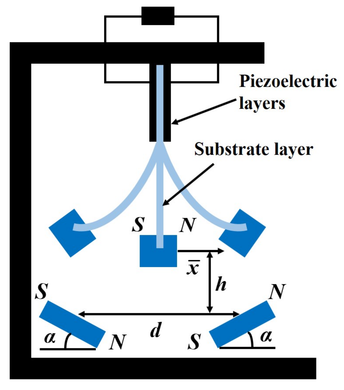
The schematic diagram of a piezoelectric cantilever vibration energy harvester [24] is shown in Figure 1. The mechanical part consists of a vertical cantilever beam with a tip magnet and two external magnets located symmetrically near the free of the metal substrate. Two piezoceramic layers are attached onto the root of cantilever beam. Under external excitations, the beam vibrates in the magnetic field created by the two external magnets and a tip magnet, which leads to the physical deformation of piezoelectric materials near the free end of cantilever beam. Due to the polarization phenomenon induced by piezoelectric effect, the opposite charges are generated on the upper and lower surfaces of piezoelectric materials, resulting in the output voltage, which realizes the conversion from ambient vibrations to the electrical energy.

Adjusting the magnetoelastic interaction depending on the distance h between the tip magnet and external magnets, the distance d between the two external magnets and angle $\alpha$ of the external magnets in a vertical direction, the energy harvester may have one, three (with one stable) or five (with three stable) equilibrium positions. Among these, the TEH can jump among three equilibrium points at low excitation level and can realize more frequently jumping to generate higher output voltage when the external excitation intensity is fairly large. The electromechanical equations of the TEH can be expressed as

$$\left\{\begin{array}{c}m\ddot{\overline{x}}\left(t\right)+c\dot{\overline{x}}\left(t\right)+\frac{\mathrm{d}U\left(\overline{x}\right)}{\mathrm{d}\overline{x}}-\theta \overline{v}\left(t\right)=F\left(t\right),\hfill \\ C_p\dot{\overline{v}}\left(t\right)+\frac{1}{R_l}\overline{v}\left(t\right)+\theta \dot{\overline{x}}\left(t\right)=0,\hfill \end{array}\right.$$

(1)

where $\overline{x}\left(t\right)$, m and c are the tip displacement in the transverse direction, the equivalent mass and the equivalent damping, respectively; $\theta$ is the electromechanical coupling coefficient; $C_p$ is the capacitance of the piezoelectric energy harvester; $\overline{v}\left(t\right)$ is the output voltage measured across the load resistance $R_l$; $F\left(t\right)$ is the external mechanical force as the excitation term. The potential function $U\left(\overline{x}\right)$, which depends on the tip displacement, has the following form

$$U\left(\overline{x}\right)=\frac{1}{2}{k}_1{\overline{x}}^2+\frac{1}{4}{k}_3{\overline{x}}^4+\frac{1}{6}{k}_5{\overline{x}}^6,$$

(2)

where $k_1,$$k_3$ and $k_5$ are the coefficients of nonlinear restoring forces.

For convenience, the dimensionless electromechanical equations under the periodic force $Acos\left(\omega t\right)$ [24] can be recast as follows

$$\left\{\begin{array}{c}\ddot{x}+\zeta \dot{x}+x+\lambda x^3+\mu x^5-\alpha v=Acos\left(\omega t\right),\hfill \\ \dot{v}+\beta v+\alpha \dot{x}=0,\hfill \end{array}\right.$$

(3)

where $\zeta ,$$\lambda$ and $\mu$ represent the mechanical damping ratio, the coefficient of the dimensionless cubic nonlinearity and dimensionless quantic nonlinearity, respectively; $\alpha$ represents the dimensionless electromechanical coupling coefficient; $\beta$ represents the ratio between the period of the mechanical system to the time constant of the harvester.

Different properties of the electromechanical model will be performed on account of the different values of $\lambda$ and $\mu$. When $\mu >0$ and $\lambda <-2\sqrt{\mu }$, the system (3) is a TEH. The tristable potential functions with different values of $\lambda$ and $\mu$ are shown in Figure 2, which have one middle potential well and two symmetric potential wells on both sides. Moreover, the potential well barrier of two symmetric potential wells becomes smaller with the increasing of the values of $\lambda$ and $\mu$, yet there are small variations for the depth and width of middle potential well. Because the interwell high energy motion requires overcoming the barrier between two potential wells to enhance energy harvesting performance, the influence of nonlinear coefficients $\lambda$ and $\mu$ on the dynamic responses of the TEH should be considered.

3. The Approximation of the TEH with an Uncertain Parameter

At present, there are three basic mathematical methods available to solve the system response with uncertain parameters, namely, Monte-Carlo method, stochastic perturbation method and orthogonal polynomial approximation method. Among them, the orthogonal polynomial approximation method not requires the assumption of small random perturbation and can achieve a high locating accuracy. Hence, the orthogonal polynomial approximation method is adopted to investigate the stochastic response of the TEH with an uncertain parameter in this research.

3.1. Chebyshev Polynomial Approximation

Uncertain parameters for engineering structures are bounded in reality. The arch-like probability density function is one of the reasonable probability density function (PDF) models for the bounded random variables, which can be described as follows

$$p\left(\xi \right)=\left\{\begin{array}{cc}\hfill \frac{2}{\pi }\sqrt{1-{\xi }^2}& \left|\xi \right|\le 1,\\ \hfill 0& \left|\xi \right|>1.\end{array}\right.$$

(4)

As the orthogonal polynomial basis for the arch-like PDF of $\xi$, the relevant polynomials are the second kind of Chebyshev polynomials which can be expressed as

$$H_n\left(\xi \right)=\sum _{k=0}^{\left[n/2\right]}{\left(-1\right)}^k\frac{\left(n-k\right)!}{k!\left(n-2k\right)!}{\left(2\xi \right)}^{n-2k},n=0,1,\cdots .$$

(5)

While the corresponding recurrence formula is

$$\xi H_n\left(\xi \right)=\frac{1}{2}\left[H_{n-1}\left(\xi \right)+H_{n+1}\left(\xi \right)\right].$$

(6)

The orthogonality for the second kind of Chebyshev polynomials can be derived as

$${\int }_{-1}^1\frac{2}{\pi }\sqrt{1-{\xi }^2}{H}_i\left(\xi \right)H_j\left(\xi \right)\mathrm{d}\xi =\left\{\begin{array}{cc}\hfill 1& i=j,\\ \hfill 0& i\ne j.\end{array}\right.$$

(7)

According to the theory of functional analysis, any measurable function $f\left(x\right)$ can be expressed into the following series form

$$f\left(\xi \right)=\sum _{i=0}^N{f}_i{H}_i\left(\xi \right),$$

(8)

where the subscript i runs for the sequential number of Chebyshev polynomials, N represents the largest order of the polynomials we have given, $f_i$ can be expanded as

$$f_i={\int }_{-1}^{1}p\left(\xi \right)f\left(\xi \right)H_i\left(\xi \right)\mathrm{d}\xi .$$

(9)

This expansion is the orthogonal decomposition of measurable function $f\left(\xi \right)$, which is the theoretical base of orthogonal decomposition methods.

3.2. Equivalent Deterministic System

There is no doubt that the errors in manufacturing and installation of TEHs cannot be totally eliminated, particularly for the distance between the tip magnet and external magnets, the distance between two external magnets and the angle of external magnets. These uncertain variables are closely related to the potential function, and therefore we set the coefficient $\lambda$ of the potential function as an uncertain parameter, which is expressed as

$$\lambda =\overline{\lambda }+\sigma \xi ,$$

(10)

where $\overline{\lambda }$ is the mean value of $\lambda$; $\xi$ is a bounded random variable defined on $\left[-1,1\right]$ with the probability density function $p\left(\xi \right)$, which has been given in Equation (4); $\sigma$ is the intensity of $\lambda$.

Then, the dimensionless electromechanical equations of TEH with an uncertain parameter can be written as follows

$$\left\{\begin{array}{c}\ddot{x}\left(t\right)+\zeta \dot{x}\left(t\right)+x\left(t\right)+\left(\overline{\lambda }+\sigma \xi \right){x\left(t\right)}^3+\mu {x\left(t\right)}^5-\alpha v\left(t\right)=Acos\left(\omega t\right),\hfill \\ \dot{v}\left(t\right)+\beta v\left(t\right)+\alpha \dot{x}\left(t\right)=0.\hfill \end{array}\right.$$

(11)

According to the theory of orthogonal polynomial approximation above, the responses of Equation (11) can be expressed by the following series

$$\left\{\begin{array}{c}\hfill x\left(t,\xi \right)={\displaystyle \sum _{i=0}^N}{x}_i\left(t\right)H_i\left(\xi \right),\\ \hfill v\left(t,\xi \right)={\displaystyle \sum _{i=0}^N}{v}_i\left(t\right)H_i\left(\xi \right),\end{array}\right.$$

(12)

where $x_i\left(t\right)$ and $v_i\left(t\right)$ can be obtained by Equation (9). While $N\to \infty$, ${\displaystyle \sum _{i=0}^N}{x}_i\left(t\right)H_i\left(\xi \right)$ and ${\displaystyle \sum _{i=0}^N}{v}_i\left(t\right)H_i\left(\xi \right)$ are strictly equivalent to $x\left(t,\xi \right)$ and $v\left(t,\xi \right)$. To meet the needs of the calculation efficiency, we take $N=4$ in Equation (12), then

$$\left\{\begin{array}{c}x\left(t,\xi \right)\approx {\displaystyle \sum _{i=0}^4}{x}_i\left(t\right)H_i\left(\xi \right),\hfill \\ v\left(t,\xi \right)\approx {\displaystyle \sum _{i=0}^4}{v}_i\left(t\right)H_i\left(\xi \right),\hfill \end{array}\right.$$

(13)

which are approximate solutions with a minimal mean square residual error. Substituting Equation (13) into Equation (11), yields

$$\left\{\begin{array}{c}{\displaystyle \sum _{i=0}^4}{\ddot{x}}_i\left(t\right)H_i\left(\xi \right)+\zeta {\displaystyle \sum _{i=0}^4}{\dot{x}}_i\left(t\right)H_i\left(\xi \right)+{\displaystyle \sum _{i=0}^4}{x}_i\left(t\right)H_i\left(\xi \right)+\overline{\lambda }{\left[{\displaystyle \sum _{i=0}^4}{x}_i\left(t\right)H_i\left(\xi \right)\right]}^3+\sigma \xi {\left[{\displaystyle \sum _{i=0}^4}{x}_i\left(t\right)H_i\left(\xi \right)\right]}^3\hfill \\ +\mu {\left[{\displaystyle \sum _{i=0}^4}{x}_i\left(t\right)H_i\left(\xi \right)\right]}^5-\alpha {\displaystyle \sum _{i=0}^4}{v}_i\left(t\right)H_i\left(\xi \right)=Acos\left(\omega t\right),\hfill \\ {\displaystyle \sum _{i=0}^4}{\dot{v}}_i\left(t\right)H_i\left(\xi \right)+\beta {\displaystyle \sum _{i=0}^4}{v}_i\left(t\right)H_i\left(\xi \right)+\alpha {\displaystyle \sum _{i=0}^4}{\dot{x}}_i\left(t\right)H_i\left(\xi \right)=0.\hfill \end{array}\right.$$

(14)

Since the product of any two Chebyshev polynomials can be transformed into a linear combination of related single Chebyshev polynomials, the cubic term and quantic term can be reduced as

$${\left[{\displaystyle \sum _{i=0}^4}{x}_i\left(t\right)H_i\left(\xi \right)\right]}^3={\displaystyle \sum _{i=0}^{12}}{X}_i\left(t\right)H_i\left(\xi \right),$$

(15)

$${\left[{\displaystyle \sum _{i=0}^4}{x}_i\left(t\right)H_i\left(\xi \right)\right]}^5={\displaystyle \sum _{i=0}^{20}}{Y}_i\left(t\right)H_i\left(\xi \right).$$

(16)

Moreover, according to recurrent formulas (6) of the Chebyshev polynomials,

$\sigma \xi {\left[{\displaystyle \sum _{i=0}^4}{x}_i\left(t\right)H_i\left(\xi \right)\right]}^3$ in Equation (14) can be reduced to

$$\begin{array}{cc}\hfill \sigma \xi {\left[{\displaystyle \sum _{i=0}^4}{x}_i\left(t\right)H_i\left(\xi \right)\right]}^3=\sigma \xi {\displaystyle \sum _{i=0}^{12}}{X}_i\left(t\right)H_i\left(\xi \right)& =\frac{1}{2}\sigma \sum _{i=0}^{12}{X}_i\left(t\right)\left[H_{i-1}\left(\xi \right)+H_{i+1}\left(\xi \right)\right]\hfill \\ \hfill & =\frac{1}{2}\sigma \sum _{i=0}^{12}\left[X_{i-1}\left(t\right)+X_{i+1}\left(t\right)\right]H_i\left(\xi \right),\hfill \end{array}$$

(17)

where $X_{-1}\left(t\right)$ and $X_5\left(t\right)$ are supposed to be zero. Substituting expressions (15), (16) and (17) into Equation (14), we have

$$\left\{\begin{array}{c}{\displaystyle \sum _{i=0}^4}{\ddot{x}}_i\left(t\right)H_i\left(\xi \right)+\zeta {\displaystyle \sum _{i=0}^4}{\dot{x}}_i\left(t\right)H_i\left(\xi \right)+{\displaystyle \sum _{i=0}^4}{x}_i\left(t\right)H_i\left(\xi \right)+\overline{\lambda }{\displaystyle \sum _{i=0}^{12}}{X}_i\left(t\right)H_i\left(\xi \right)+\hfill \\ \frac{1}{2}\sigma {\displaystyle \sum _{i=0}^{12}}\left[X_{i-1}\left(t\right)+X_{i+1}\left(t\right)\right]H_i\left(\xi \right)+\mu {\displaystyle \sum _{i=0}^{20}}{Y}_i\left(t\right)H_i\left(\xi \right)-\alpha {\displaystyle \sum _{i=0}^4}{v}_i\left(t\right)H_i\left(\xi \right)=Acos\left(\omega t\right),\hfill \\ {\displaystyle \sum _{i=0}^4}{\dot{v}}_i\left(t\right)H_i\left(\xi \right)+\beta {\displaystyle \sum _{i=0}^4}{v}_i\left(t\right)H_i\left(\xi \right)+\alpha {\displaystyle \sum _{i=0}^4}{\dot{x}}_i\left(t\right)H_i\left(\xi \right)=0.\hfill \end{array}\right.$$

(18)

Multiplying both sides of Equation (18) by $H_i\left(\xi \right)$ in sequence and taking expectations with respect to $\xi$, in accordance with the orthogonality of the Chebyshev polynomials, the high-dimensional equivalent system of the TEH can be written as

$$\left\{\begin{array}{c}{\ddot{x}}_0\left(t\right)+\zeta {\dot{x}}_0\left(t\right)+x_0\left(t\right)+\overline{\lambda }{X}_0\left(t\right)+\frac{1}{2}\sigma X_1\left(t\right)+\mu Y_0\left(t\right)-\alpha v_0\left(t\right)=Acos\left(\omega t\right),\hfill \\ {\dot{v}}_0\left(t\right)+\beta v_0\left(t\right)+\alpha {\dot{x}}_0\left(t\right)=0,\hfill \\ {\ddot{x}}_1\left(t\right)+\zeta {\dot{x}}_1\left(t\right)+x_1\left(t\right)+\overline{\lambda }{X}_1\left(t\right)+\frac{1}{2}\sigma \left[X_0\left(t\right)+X_2\left(t\right)\right]+\mu Y_1\left(t\right)-\alpha v_1\left(t\right)=0,\hfill \\ {\dot{v}}_1\left(t\right)+\beta v_1\left(t\right)+\alpha {\dot{x}}_1\left(t\right)=0,\hfill \\ {\ddot{x}}_2\left(t\right)+\zeta {\dot{x}}_2\left(t\right)+x_2\left(t\right)+\overline{\lambda }{X}_2\left(t\right)+\frac{1}{2}\sigma \left[X_1\left(t\right)+X_3\left(t\right)\right]+\mu Y_2\left(t\right)-\alpha v_2\left(t\right)=0,\hfill \\ {\dot{v}}_2\left(t\right)+\beta v_2\left(t\right)+\alpha {\dot{x}}_2\left(t\right)=0,\hfill \\ {\ddot{x}}_3\left(t\right)+\zeta {\dot{x}}_3\left(t\right)+x_3\left(t\right)+\overline{\lambda }{X}_3\left(t\right)+\frac{1}{2}\sigma \left[X_2\left(t\right)+X_4\left(t\right)\right]+\mu Y_3\left(t\right)-\alpha v_3\left(t\right)=0,\hfill \\ {\dot{v}}_3\left(t\right)+\beta v_3\left(t\right)+\alpha {\dot{x}}_3\left(t\right)=0,\hfill \\ {\ddot{x}}_4\left(t\right)+\zeta {\dot{x}}_4\left(t\right)+x_4\left(t\right)+\overline{\lambda }{X}_4\left(t\right)+\frac{1}{2}\sigma X_3\left(t\right)+\mu Y_4\left(t\right)-\alpha v_4\left(t\right)=0,\hfill \\ {\dot{v}}_4\left(t\right)+\beta v_4\left(t\right)+\alpha {\dot{x}}_4\left(t\right)=0,\hfill \end{array}\right.$$

(19)

which is a kind of weighted average system. So the ensemble mean response (EMR) of the TEH with an uncertain parameter can be introduced to reflect the average characteristics of the original system (11), that is

$$\left\{\begin{array}{c}E\left[x\left(t,\xi \right)\right]=E\left[{\displaystyle \sum _{i=0}^4}{x}_i\left(t\right)H_i\left(\xi \right)\right]=x_0\left(t\right),\hfill \\ E\left[v\left(t,\xi \right)\right]=E\left[{\displaystyle \sum _{i=0}^4}{v}_i\left(t\right)H_i\left(\xi \right)\right]=v_0\left(t\right).\hfill \end{array}\right.$$

(20)

3.3. Validation

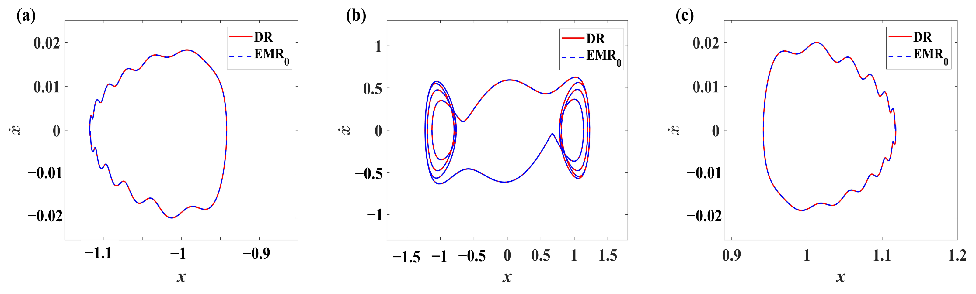
In this section, we focus on to verify the effectiveness of the Chebyshev polynomial approximation. The deterministic response (DR) of system (3) and the deterministic ensemble mean response (EMR${}_0$) of system (19) by setting the stochastic intensity $\sigma =0.0$ in Equation (19) can be obtained numerically. Here the parameters of system (3) and (19) are choosen as $\zeta =0.02,$$\mu =3.5,$$\alpha =0.9,$$A=0.5,$$\omega =0.2,$$\beta =0.5,$$\sigma =0.0$ and $\lambda =\overline{\lambda }=-4.82$. The phase portraits of DR and EMR${}_0$ under different initial conditions are shown in Figure 3. It can be seen that DR and EMR${}_0$ coincide with each other very well, which illustrates the validity of the Chebyshev polynomial approximation for the TEH with an uncertain parameter.

4. Parametric Uncertainty Analysis

In this section, EMR of the equivalent system (19) is compared with DR of deterministic system (3) to reveal the dynamic characteristics of stochastic TEH and the influence of uncertain parameter $\lambda$ on the energy harvesting performance.

4.1. Influence of the Damping Coefficient

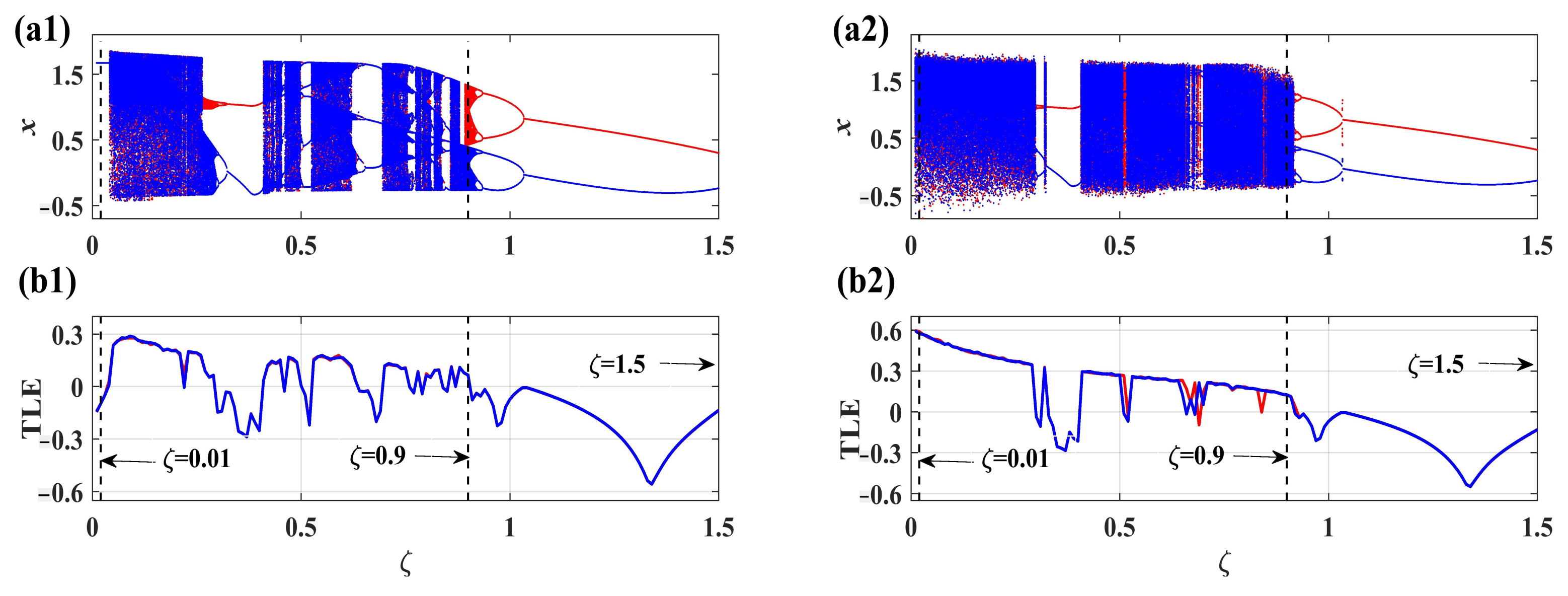
In system (3), the parameters are chosen as $\lambda =-4.5,$$\mu =2.5,$$\alpha =0.9,$$A=2.8,$$\omega =0.8$ and $\beta =0.5$. When the damping coefficient $\zeta$ varies from 1.5 to 0.0, the multivalued bifurcation diagram and the top Lyapunov exponent (TLE) of DR are obtained by selecting different initial conditions, as shown in Figure 4(a1,b1). When $\zeta =1.5$, it can be seen that there exist two 1T-period attractors. After $\zeta$ decreases to the critical value about $\zeta =1.03$, the system responses go to chaotic motion through the period doubling bifurcation cascade. Moreover, as $\zeta$ decreases from 1.03 to 0.04, the system undergoes several period doubling bifurcation cascades, crises and periodic motions. Furthermore, we find a typical crisis near $\zeta =0.04$, where the chaotic attractor is suddenly destroyed and replaced by a newborn regular 1T-period attractor.

Based on the above deterministic analysis, we take $\overline{\lambda }=4.5$, $\sigma =0.01$ in the system (19) to investigate the influence of uncertain parameter. The multivalued bifurcation diagram and corresponding TLE of EMR are plotted in Figure 4(a2,b2), from which we can see that the global stochastic dynamics of system (19) is similar to the deterministic case in Figure 4(a1,b1). However, there are still some different stochastic properties in details, which are presented as follows.

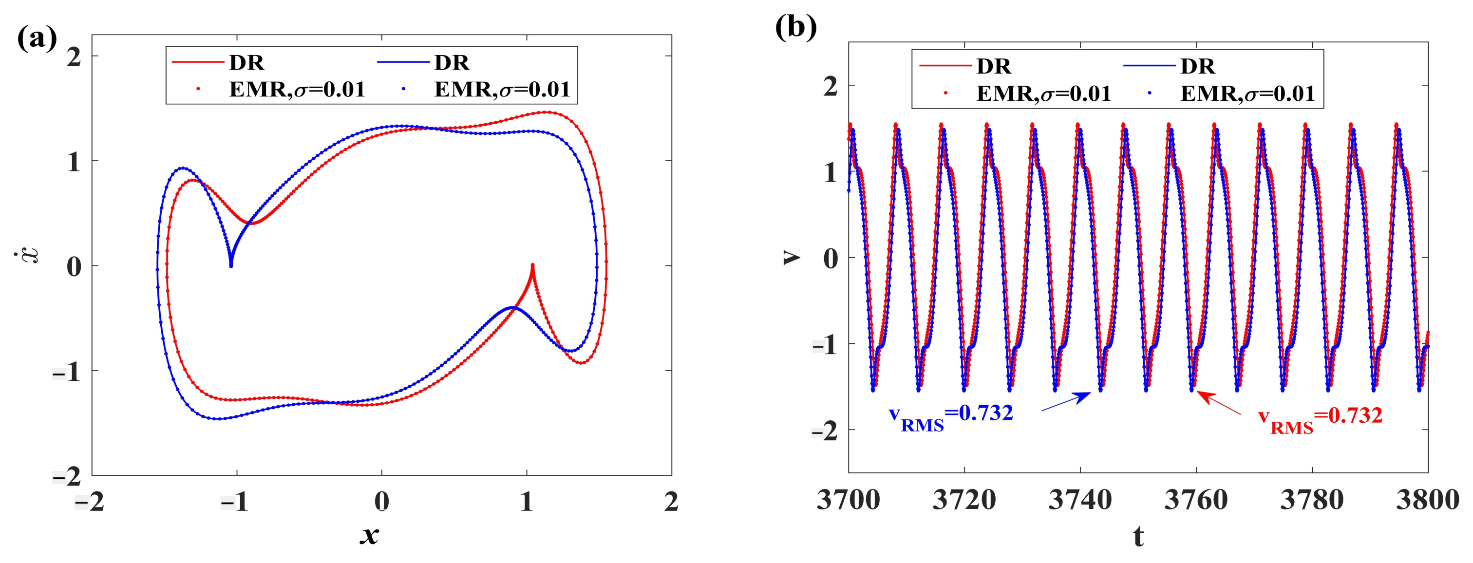
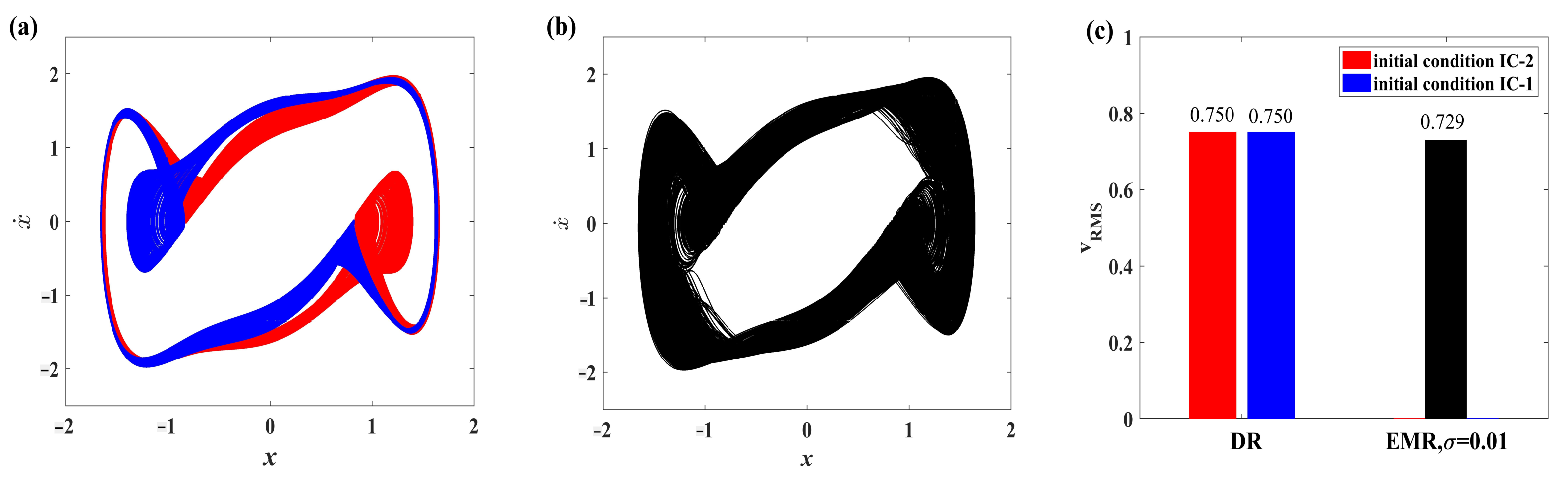
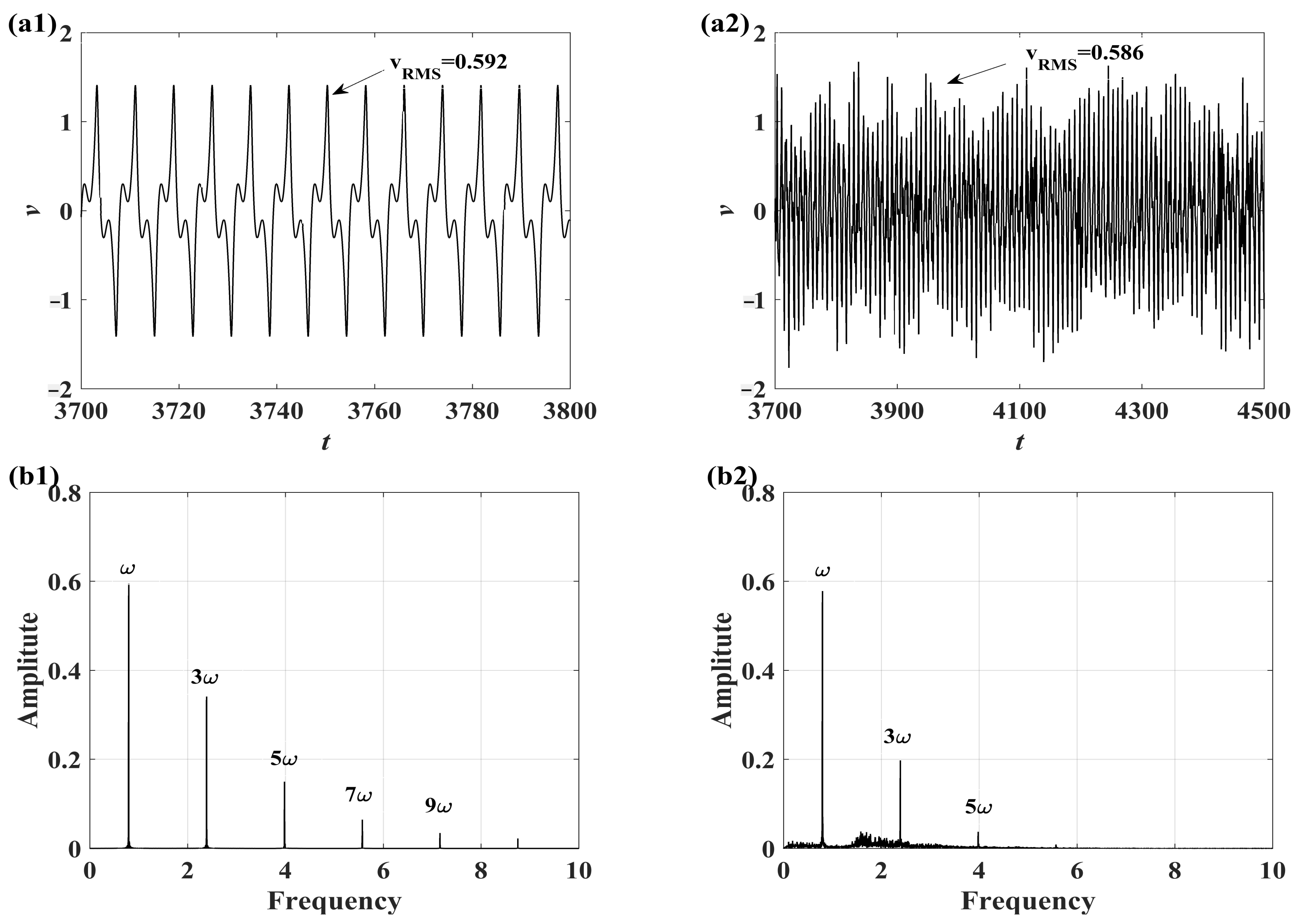
Now let $\zeta =1.5$, the DR and EMR with $\sigma =0.01$ are shown in Figure 5. It can be observed that DR and EMR are 1T-period under two different initial conditions and the output voltages are stable. The root mean square (RMS) voltages of DR and EMR are 0.732. For $\zeta =0.9$, there are two chaotic attractors for DR in Figure 6. Because of the occurrence of the merging crisis, two chaotic attractors turn into a greater chaotic attractor for EMR with $\sigma =0.01$ and the RMS voltages reduce from 0.750 to 0.729. When $\zeta =0.02$, DR is periodic and discrete spectrums can be viewed in Figure 7(b1). However, EMR becomes chaotic due to the influence of uncertain parameter, which can be illustrated from the continuous spectrum of the output voltage over a wide range of frequency in Figure 7(b2). Compared with DR, the amplitudes of frequency components of EMR decrease, especially in the frequencies $3\omega$ and $5\omega$.

The stochastic behavior of TEH with $\sigma =0.01$ has been investigated above. Then, different values of $\sigma$ are employed to observe how is about the influence under different intensities. It is clearly that the bigger the intensity $\sigma$ is, the wider the interval matching the positive TLE of EMR is, as shown in Figure 8.

4.2. Influence of the Electromechanical Coupling Coefficient

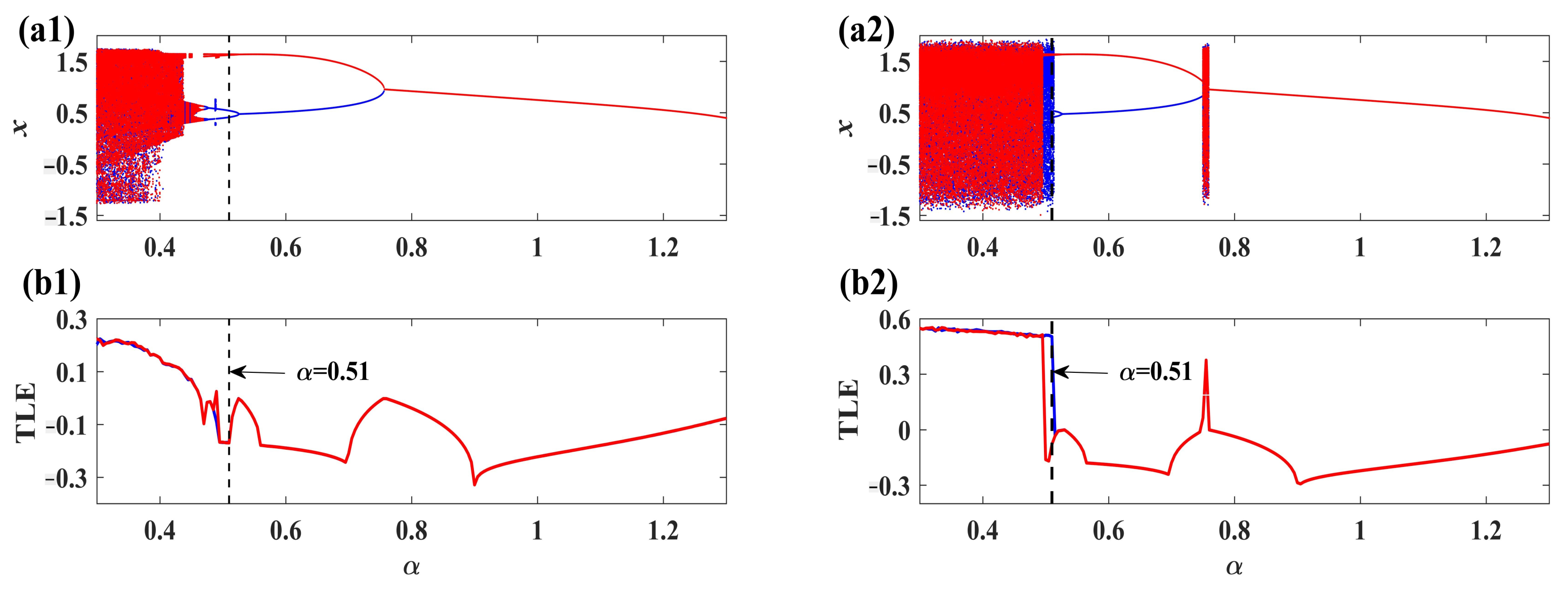
The electromechanical coupling coefficient $\alpha$ plays a key role in the behavior of TEH, so we consider $\alpha$ as the bifurcation parameter. Let $\lambda =-4.5,$$\overline{\lambda }=-4.5,$$\mu =2.5,$$\zeta =0.2,$$A=1.2,$$\omega =0.9,$$\beta =0.5$ and $\sigma =0.01$, the multivalued bifurcation diagrams and corresponding TLE of DR and EMR are shown in Figure 9(a1,a2), respectively. When $\alpha \approx 0.77$, DR keeps the periodic motion, but EMR enters into transient chaotic motion on account of the influence of the uncertain parameter. After $\alpha$ decreases to the critical value about $\alpha \approx 0.52$, DR undergoes several period doubling bifurcation cascades and finally becomes chaotic in Figure 9(a1), where the corresponding TLE of DR gradually changes from negative to positive. Instead, the crisis from periodic to chaotic motion can be clearly observed for EMR and the TLE of EMR suddenly changes from negative to positive within $0.46\le \alpha \le 0.52$. Besides, the harvester under the initial condition IC-3 leaves the chaotic region firstly, which can be seen more clearly in Figure 9(b2).

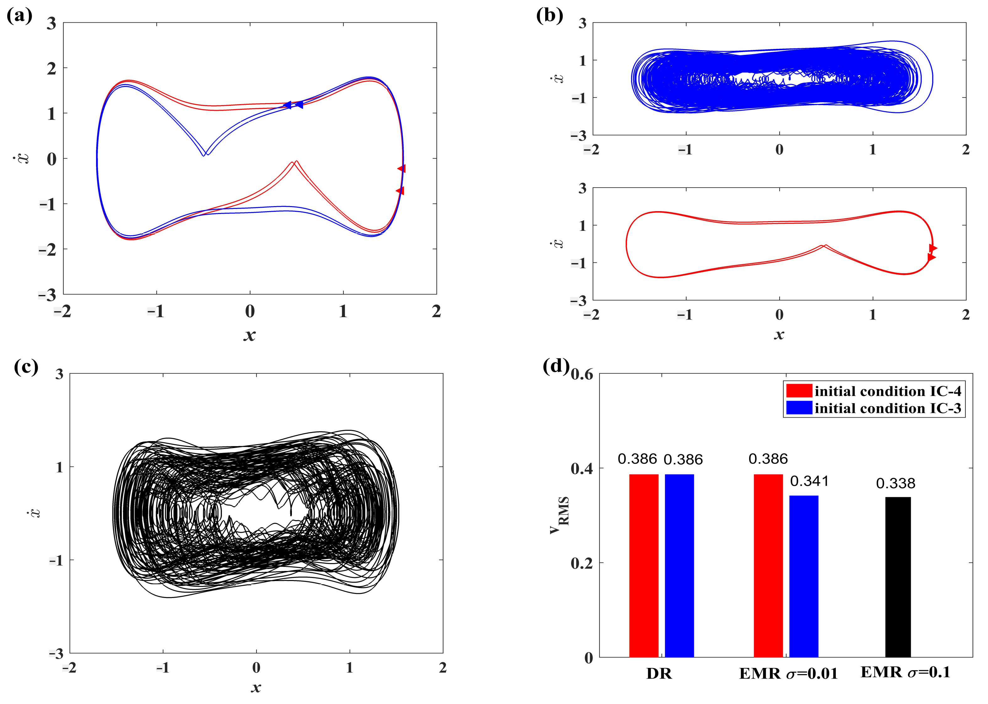
Especially, when $\alpha =0.51$, DR keeps 2T-period motion for different initial conditions in Figure 10a. As we take the stochastic intensity $\sigma =0.01$ in Figure 10b, there is almost no distinction between DR and EMR with the initial condition IC-4, but EMR with the initial condition IC-3 becomes chaotic. This indicates that the dynamic behavior of TEH is sensitive to the initial conditions around the given parameters. Furthermore, as $\sigma$ is increased to 0.1 in Figure 10c, the system responses of harvester enter into the chaotic motion under two different initial conditions, which make the output voltages unstable. In addition, the RMS voltages of DR and EMR are calculated in Figure 10d, where EMR($\sigma =0.01$) under the initial condition IC-3 generates $11.6\%$ smaller RMS voltage and EMR($\sigma =0.1$) generates $12.4\%$ smaller RMS voltage.

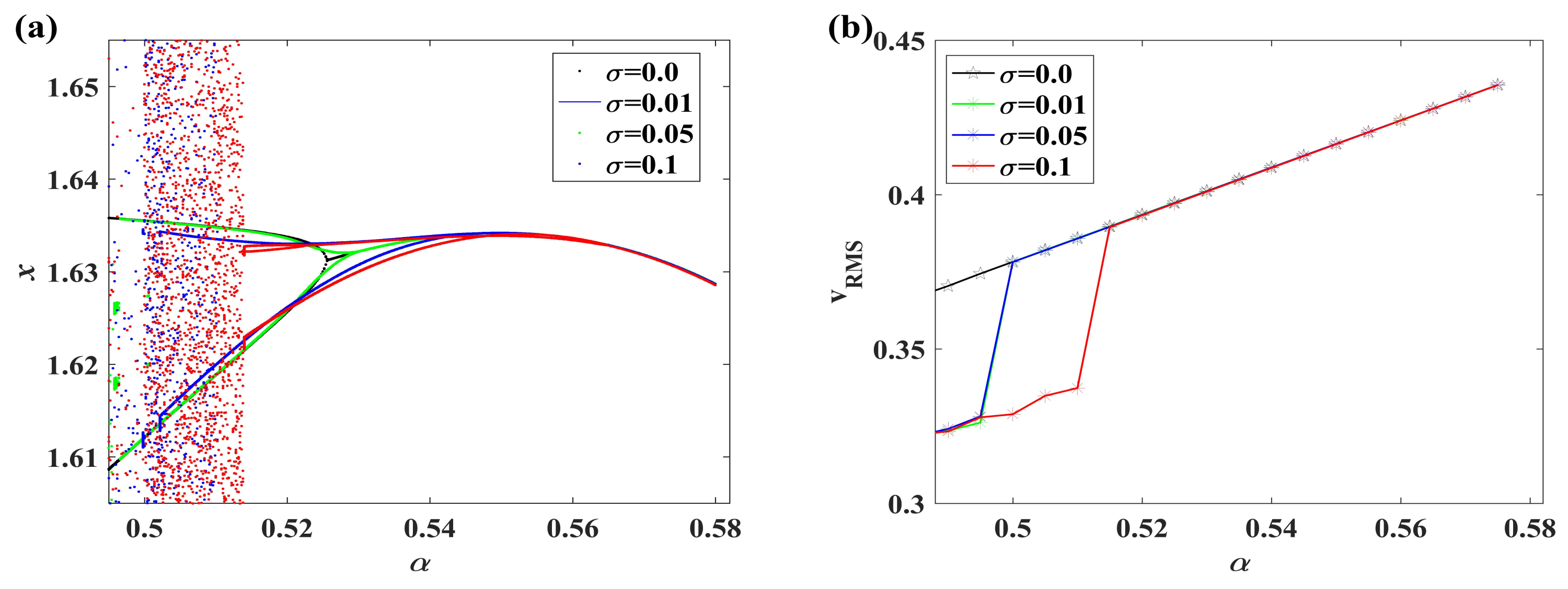
From the above analysis, we find that the stochastic dynamics phenomenon of the TEH can be affected more by the bigger intensity of uncertain parameter. For this reason, and then taking the values of intensity $\sigma$ as 0.0, 0.01, 0.05 and 0.1, the bifurcation diagrams and RMS voltage under the initial condition IC-4 within $0.5<\alpha <0.58$ are investigated. It can be observed that the critical interval of stochastic period-doubling bifurcation cascade shifts ahead with the increasing of $\sigma$ in Figure 11a. Moreover, the RMS voltage within $\alpha <0.52$ is smaller than that in the case of deterministic form in Figure 11b. In addition, when $0.52<\alpha <0.58$, these RMS values under the stochastic intensities $\sigma =0.01,0.05$ and $0.1$ do not change considerably.

4.3. Combined Influence of the Damping Coefficient and Electromechanical Coupling Coefficient

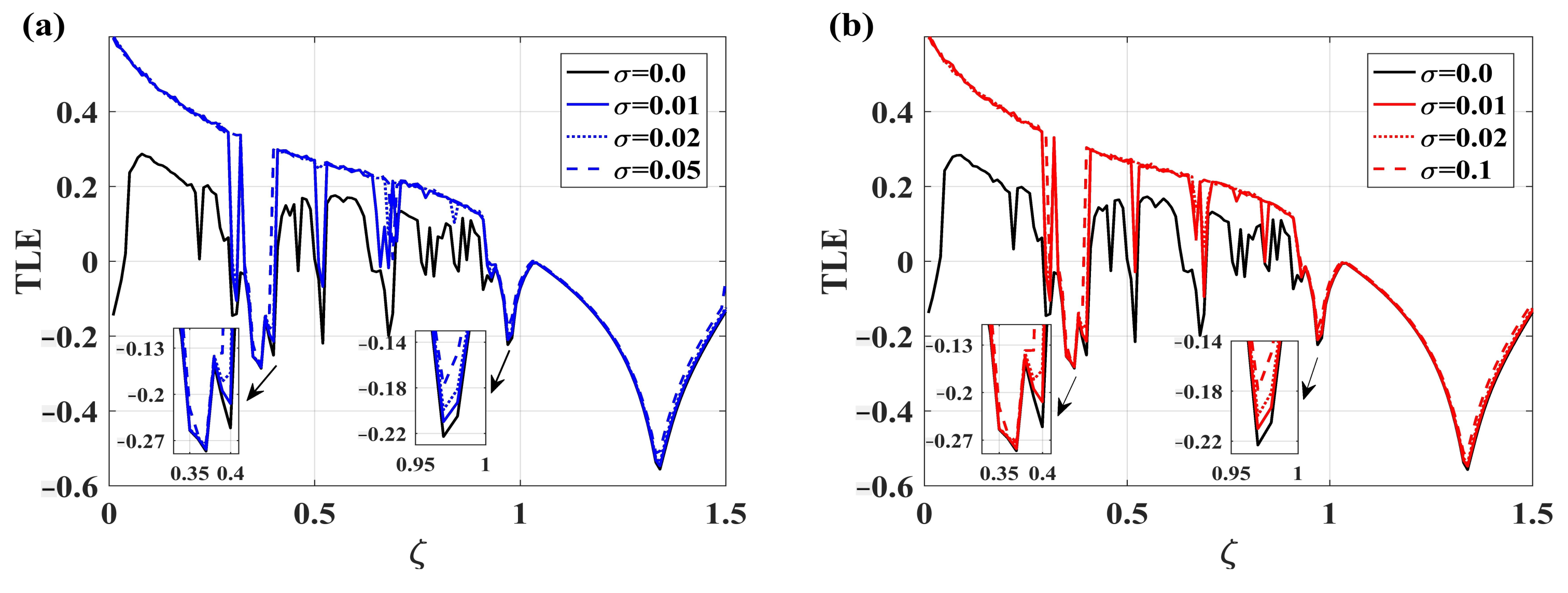
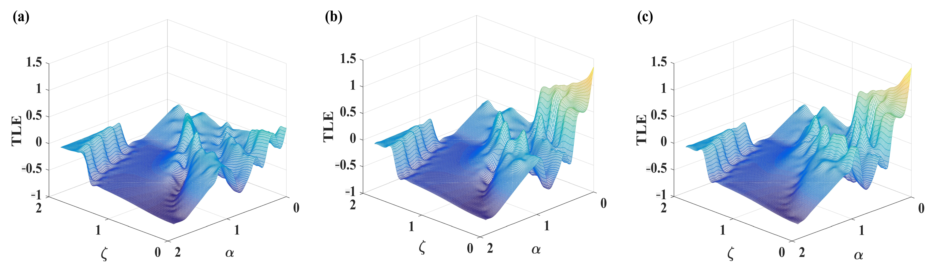
In order to show the combined influence of uncertain parameter $\alpha$ on the damping coefficient and electromechanical coupling coefficient, the TLEs with the variation of $\zeta$ and $\alpha$ under different intensities $\sigma$ are presented in Figure 12. Other parameters in system (19) are set to $\overline{\lambda }=-4.5,$$\mu =2.5,$$\zeta =0.2,$$\alpha =0.9,$$A=1.2,$$\omega =0.9$ and $\beta =0.5$.

For $\sigma$ = 0.0, the TLEs keep negative at most points of the region $\left\{(\zeta ,\alpha )|0<\zeta <2,0<\alpha <2\right\}$, which means that responses of harvester are almost always in the state of periodic motion. As $\sigma$ increases to 0.01, there are some more positive TLEs for smaller damping coefficient $\zeta$ and smaller electromechanical coupling coefficient $\alpha$ occurred in Figure 12b, where the fluctuation of TLE is obvious. Furthermore, when $\sigma$ increases from 0.01 to 0.05, the surface of the TLE becomes more unsmooth and more positive TLEs can be found in Figure 12c. These illustrate that the motion of harvester becomes more complex with the increasing of $\sigma$. Thus, the uncertainty could not be ignored in the TEH and we should control the randomness at a rather smaller level to reduce the influence of the uncertain parameter.

5. Conclusions

In this paper, the dynamic behaviors of the TEH with uncertain parameter are explored. Chebyshev polynomial approximation method is applied to transform the stochastic TEH into that of a deterministic system. The ensemble mean response of this deterministic system can be obtained, and the validity of this method is verified by the numerical simulation. The influences of uncertain parameter on the TEH system are studied by analyzing the bifurcation diagram, the top Lyapunov exponent and the time-history diagram.

The results illustrate that the TEH with uncertain parameter keeps similar global dynamics with the original system in the large periodic windows. Nevertheless, under the influence of random coefficient ahead of the nonlinear term, the parameter intervals for chaotic behavior diffuse into wider ones. With the increasing of intensity of the random coefficient, the chaotic ranges become wider and wider. Meanwhile, stochastic responses are much more sensitive around the period-doubling bifurcation and crisis critical points about the damping and electromechanical coupling coefficients. That can make the output voltage leave from the large-amplitude periodic fluctuation, and therefore reduce the energy harvesting efficiency. Consequently, the structural uncertainties should be paid more attention in design, and the system parameters should be selected from stable intervals of the output voltage.

References

- Beeby, S.P.; Tudor, M.J.; White, N.M. Energy harvesting vibration sources for microsystems applications. Meas. Sci. Technol. 2006, 17, R175. [Google Scholar] [CrossRef]
- Erturk, A.; Hoffmann, J.; Inman, D.J. A piezomagnetoelastic structure for broadband vibration energy harvesting. Appl. Phys. Lett. 2009, 94, 254102. [Google Scholar] [CrossRef]
- Akaydin, H.D.; Elvin, N.; Andreopoulos, Y. Energy harvesting from highly unsteady fluid flows using piezoelectric materials. J. Intell. Mater. Syst. Struct. 2010, 21, 1263–1278. [Google Scholar] [CrossRef]
- Cottone, F.; Vocca, H.; Gammaitoni, L. Nonlinear energy harvesting. Phys. Rev. Lett. 2012, 102, 080601. [Google Scholar] [CrossRef] [PubMed] [Green Version]
- Erturk, A.; Inman, D.J. Piezoelectric Energy Harvesting; Wiley: Hoboken, NJ, USA, 2011. [Google Scholar]
- Beeby, S.P.; Torah, R.N.; Tudor, M.J.; Glynne-Jones, P.; O’Donnell, T.; Saha, C.R.; Roy, S. A micro electromagnetic generator for vibration energy harvesting. J. Micromech. Microeng. 2007, 17, 1257–1265. [Google Scholar] [CrossRef]
- Duan, X.J.; Cao, D.X.; Li, X.G.; Shen, Y.J. Design and dynamic analysis of integrated architecture for vibration energy harvesting including piezoelectric frame and mechanical amplifier. Appl. Math. Mech. Ed. 2021, 42, 755–770. [Google Scholar] [CrossRef]
- Lu, Z.Q.; Li, K.; Ding, H.; Chen, L.Q. Nonlinear energy harvesting based on a modified snap-through mechanism. Appl. Math. Mech. Ed. 2019, 40, 167–180. [Google Scholar] [CrossRef]
- Mcinnes, C.R.; Gorman, D.G.; Cartmell, M.P. Enhanced vibrational energy harvesting using nonlinear stochastic resonance. J. Sound Vib. 2008, 318, 655–662. [Google Scholar] [CrossRef] [Green Version]
- Jin, Y.F.; Xiao, S.M.; Zhang, Y.X. Enhancement of tristable energy harvesting using stochastic resonance. J. Stat. Mech. Theory Exp. 2018, 2018, 123211. [Google Scholar] [CrossRef]
- Zhang, W.; Yao, Z.G.; Yao, M.H. Periodic and chaotic dynamics of composite laminated piezoelectric rectangular plate with one-to-two internal resonance. Sci. China Ser. E 2009, 52, 731–742. [Google Scholar] [CrossRef]
- Zhang, Y.; Jiao, Z.R.; Duan, X.X.; Xu, Y. Stochastic dynamics of a piezoelectric energy harvester with fractional damping under Gaussian colored noise excitation. Appl. Math. Model. 2021, 97, 268–280. [Google Scholar] [CrossRef]
- Yang, Y.G.; Xu, W. Stochastic analysis of monostable vibration energy harvesters with fractional derivative damping under gaussian white noise excitation. Nonlinear Dyn. 2018, 94, 639–648. [Google Scholar] [CrossRef]
- Mann, B.P.; Sims, N.D. Energy harvesting from the nonlinear oscillations of magnetic levitation. J. Sound Vib. 2009, 319, 515–530. [Google Scholar] [CrossRef] [Green Version]
- Stanton, S.C.; Mcgehee, C.C.; Mann, B.P. Reversible hysteresis for broadband magnetopiezoelastic energy harvesting. Appl. Phys. Lett. 2009, 95, 174103. [Google Scholar] [CrossRef]
- Xu, M.; Jin, X.L.; Wang, Y.; Huang, Z.L. Stochastic averaging for nonlinear vibration energy harvesting system. Nonlinear Dyn. 2014, 78, 1451–1459. [Google Scholar] [CrossRef]
- Jiang, W.A.; Sun, P.; Zhao, G.L.; Chen, L.Q. Path integral solution of vibratory energy harvesting systems. Appl. Math. Mech. (Engl. Ed.) 2019, 40, 579–590. [Google Scholar] [CrossRef]
- Yao, M.H.; Liu, P.F.; Wang, H.B. Nonlinear dynamics and power generation on a new bistable piezoelectric-electromagnetic energy harvester. Complexity 2020, 2020, 5681703. [Google Scholar] [CrossRef]
- Sun, S.; Cao, S.Q. Dynamic modeling and analysis of a bistable piezoelectric cantilever power generation system. Acta Phys. Sin. 2012, 61, 210505. [Google Scholar]
- Liu, D.; Wu, Y.R.; Xu, Y.; Li, J.L. Stochastic response of bistable vibration energy harvesting system subject to filtered gaussian white noise. Mech. Syst. Signal Process. 2019, 130, 201–212. [Google Scholar] [CrossRef]
- Liu, D.; Xu, Y.; Li, J.L. Probabilistic response analysis of nonlinear vibration energy harvesting system driven by Gaussian colored noise. Chaos Solitons Fractals 2017, 104, 806–812. [Google Scholar] [CrossRef]
- Ghandchi, T.M.; Elliott, S.J. Extending the dynamic range of an energy harvester using nonlinear damping. J. Sound Vib. 2014, 333, 623–629. [Google Scholar] [CrossRef]
- Zhou, S.X.; Cao, J.Y.; Inman, D.J.; Lin, J.; Liu, S.S.; Wang, Z.Z. Broadband tristable energy harvester: Modeling and experiment verification. Appl. Energy 2014, 133, 33–39. [Google Scholar] [CrossRef]
- Cao, J.Y.; Zhou, S.X.; Wang, W.; Lin, J. Influence of potential well depth on nonlinear tristable energy harvesting. Appl. Phys. Lett. 2015, 106, 515–530. [Google Scholar] [CrossRef]
- Kim, P.; Seok, J. Dynamic and energetic characteristics of a tri-stable magnetopiezoelastic energy harvester. Mech. Mach. Theory 2015, 94, 41–63. [Google Scholar] [CrossRef]
- Li, H.T.; Qin, W.Y.; Lan, C.B.; Deng, W.Z.; Zhou, Z.Y. Dynamics and coherence resonance of tri-stable energy harvesting system. Smart Mater. Struct. 2016, 25, 015001. [Google Scholar]
- Zhang, Y.X.; Jin, Y.F. Colored levy noise induced stochastic dynamics in a tri-stable hybrid energy harvester. J. Comput. Nonlinear Dyn. 2021, 16, 041005. [Google Scholar] [CrossRef]
- Yang, T.; Cao, Q.J. Dynamics and performance evaluation of a novel tristable hybrid energy harvester for ultra-low level vibration resources. Int. J. Mech. Sci. 2019, 156, 123–136. [Google Scholar] [CrossRef]
- Ali, S.F.; Friswell, M.I.; Adhikari, S. Piezoelectric energy harvesting with parametric uncertainty. Smart Mater. Struct. 2010, 19, 105010. [Google Scholar] [CrossRef] [Green Version]
- Nanda, A.; Karami, M.A.; Singla, P. Uncertainty quantification of energy harvesting systems using method of Quadratures and maximum entropy principle. In Smart Material, Adaptive Structures and Intelligent Systems; American Society of Mechanical Engineers: New York, NY, USA, 2015. [Google Scholar]
- Franco, V.R.; Varoto, P.S. Parameter uncertainties in the design and optimization of cantilever piezoelectric energy harvesters. Mech. Syst. Signal Process. 2017, 93, 593–609. [Google Scholar] [CrossRef]
- Yoon, H.; Youn, B.D. System reliability analysis of piezoelectric vibration energy harvesting considering multiple safety events under physical uncertainty. Smart Mater. Struct. 2018, 28, 025010. [Google Scholar] [CrossRef]
- Abdelkefi, A.; Hajj, M.R.; Nayfeh, A.H. Sensitivity analysis of piezoaeroelastic energy harvesters. J. Intell. Mater. Syst. Struct. 2012, 23, 1523–1531. [Google Scholar] [CrossRef]
- Wu, F.; Gao, Q.; Xu, X.M.; Zhong, W.X. A modified computational scheme for the stochastic perturbation finite element method. Lat. Am. J. Solids Struct. 2015, 12, 2480–2505. [Google Scholar] [CrossRef] [Green Version]
- Nieto, J.J.; Khastan, A.; Ivaz, K. Numerical solution of fuzzy differential equations under generalized differentiability. Nonlinear Anal. Hybrid Syst. 2009, 3, 700–707. [Google Scholar] [CrossRef]
- Hong, L.; Jiang, J.; Sun, J.Q. Fuzzy responses and bifurcations of a forced Duffing oscillator with a triple-well potential. Int. J. Bifurc. Chaos 2015, 25, 1550005. [Google Scholar] [CrossRef]
- Li, Y.; Zhou, S.X.; Litak, G. Uncertainty analysis of bistable vibration energy harvesters based on the improved interval extension. J. Vib. Eng. Technol. 2020, 8, 297–306. [Google Scholar] [CrossRef] [Green Version]
- Chen, S.H.; Wu, J.; Chen, Y.D. Interval optimization for uncertain structures. Finite Elem. Anal. Des. 2004, 40, 1379–1398. [Google Scholar] [CrossRef]
- Huang, D.M.; Zhou, S.X.; Han, Q.; Grzegorz, L. Response analysis of the nonlinear vibration energy harvester with an uncertain parameter. Proc. Inst. Mech. Eng. Part K J. Multi-Body Dyn. 2020, 234, 393–407. [Google Scholar] [CrossRef]
- Wiener, N. The homogeneous chaos. Am. J. Math. 1938, 60, 897–936. [Google Scholar] [CrossRef]
- Sun, T.C. A finite element method for random differential equations with random coefficients. SIAM J. Numer. Anal. 1979, 16, 1019–1035. [Google Scholar] [CrossRef]
- Li, J. Stochastic Structural System-Analysis and Modeling; Science Press: Beijing, China, 1996. [Google Scholar]
- Xiu, D.B.; Karniadakis, G.E. The wiener-askey polynomial chaos for stochastic differential equations. SIAM J. Sci. Comput. 2002, 24, 619–644. [Google Scholar] [CrossRef]
- Xiu, D.B. Numerical methods for stochastic computations: A spectral method approach. Commun. Comput. Phys. 2010, 5, 242–272. [Google Scholar]
- Fang, T.; Leng, X.L.; Song, C.Q. Chebyshev polynomial approximation for dynamical response problem of random system. J. Sound Vib. 2003, 266, 198–206. [Google Scholar] [CrossRef]
- Fang, T.; Leng, X.L.; Ma, X.P.; Meng, G. λ-PDF and Gegenbauer polynomial approximation for dynamic response problems of random structures. Acta Mech. Sin. 2004, 20, 292–298. [Google Scholar]
- Ma, S.J.; Xu, W. Period-doubling bifurcation in an extended van der Pol system with bounded random parameter. Commun. Nonlinear Sci. Numer. Simul. 2008, 13, 2256–2265. [Google Scholar] [CrossRef]
- Zhao, K.Y.; Ma, S.J. Qualitative analysis of a two-group SVIR epidemic model with random effect. Adv. Differ. Equ. 2021, 2021, 1–21. [Google Scholar] [CrossRef] [PubMed]
- Wu, C.L.; Lei, Y.M.; Fang, T. Stochastic chaos in a Duffing oscillator and its control. Chaos Solitons Fractals 2006, 27, 459–469. [Google Scholar] [CrossRef]
- Sun, X.J.; Xu, W.; Ma, S.J. Period-doubling bifurcation of a double-well Duffing-van der Pol system with bounded random parameters. Acta Phys. Sin. 2006, 55, 610–616. [Google Scholar]
- Zhang, Y.; Xu, W.; Fang, T. Stochastic Hopf bifurcation and chaos of stochastic Bonhoeffer-van der Pol system via Chebyshev polynomial approximation. Appl. Math. Comput. 2007, 190, 1225–1236. [Google Scholar] [CrossRef]
Figure 1.
Schematics of a general piezoelectric energy harvester [24].
Figure 2.
Potential functions of the TEH.
Figure 3.
The phase portraits of DR and EMR. (a,b,c) are obtained under the initial conditions .
Figure 4.
Bifurcation diagrams and the TLE with the variation of damping coefficient . (a1,a2) Multivalued bifurcation diagram of DR and EMR (); (b1,b2) Multivalued TLE of DR and EMR (). The blue dots and red dots are obtained under the initial conditions (IC-1) and (IC-2), respectively.
Figure 5.
DR and EMR () for =1.5. (a) Phase portraits; (b) Time history of the output voltage. The blue dots and red dots are obtained under the initial conditions (IC-1) and (IC-2), respectively.
Figure 6.
DR and EMR () for =0.9. (a) Phase portraits of DR; (b) Phase portraits of EMR (). (c) RMS voltage of DR and EMR (). The blue dots and red dots are obtained under the initial conditions (IC-1) and (IC-2), respectively.
Figure 7.
DR and EMR () for =0.01. (a1,a2) Time history of the output voltage of DR and EMR (); (b1,b2) Spectrum of the output voltage of DR and EMR ().
Figure 8.
The TLE with the variation of damping coefficient under different intensities; (a) is obtained under the initial condition IC-1; (b) is obtained under the initial condition IC-2.
Figure 9.
Bifurcation diagrams and the TLE with the variation of electromechanical coupling coefficient . (a1,a2) Multivalued bifurcation diagram of DR and EMR (); (b1,b2) Multivalued TLE of DR and EMR (). The blue dots and red dots are obtained under the initial conditions (IC-3) and (IC-4), respectively.
Figure 10.
DR and EMR for =0.51. (a) Phase portraits of DR; (b) Phase portraits of EMR (); (c) Phase portraits of EMR (); (d) RMS voltage of DR and EMR. The blue dots and red dots are obtained under the initial conditions (IC-3) and (IC-4), respectively.
Figure 11.
EMR for 0.5 < < 0.58 under the stochastic intensities = 0.0, = 0.01, = 0.05 and = 0.1. (a) Bifurcation diagrams; (b) RMS voltage.
Figure 12.
The TLE with the variation of damping coefficient and electromechanical coupling coefficient under different intensities. (a) = 0.0; (b) = 0.01; (c) = 0.05.
Publisher’s Note: MDPI stays neutral with regard to jurisdictional claims in published maps and institutional affiliations. |
© 2021 by the authors. Licensee MDPI, Basel, Switzerland. This article is an open access article distributed under the terms and conditions of the Creative Commons Attribution (CC BY) license (https://creativecommons.org/licenses/by/4.0/).
Share and Cite
MDPI and ACS Style
Zhang, Y.; Duan, X.; Shi, Y.; Yue, X. Response Analysis of the Tristable Energy Harvester with an Uncertain Parameter. Appl. Sci. 2021, 11, 9979. https://0-doi-org.brum.beds.ac.uk/10.3390/app11219979
AMA Style
Zhang Y, Duan X, Shi Y, Yue X. Response Analysis of the Tristable Energy Harvester with an Uncertain Parameter. Applied Sciences. 2021; 11(21):9979. https://0-doi-org.brum.beds.ac.uk/10.3390/app11219979
Chicago/Turabian StyleZhang, Ying, Xiaxia Duan, Yu Shi, and Xiaole Yue. 2021. "Response Analysis of the Tristable Energy Harvester with an Uncertain Parameter" Applied Sciences 11, no. 21: 9979. https://0-doi-org.brum.beds.ac.uk/10.3390/app11219979
Note that from the first issue of 2016, this journal uses article numbers instead of page numbers. See further details here.