
Near-Surface Geological Structure Seismic Wave Imaging Using the Minimum Variance Spatial Smoothing Beamforming Method

 ,
,
Abstract
:1. Introduction
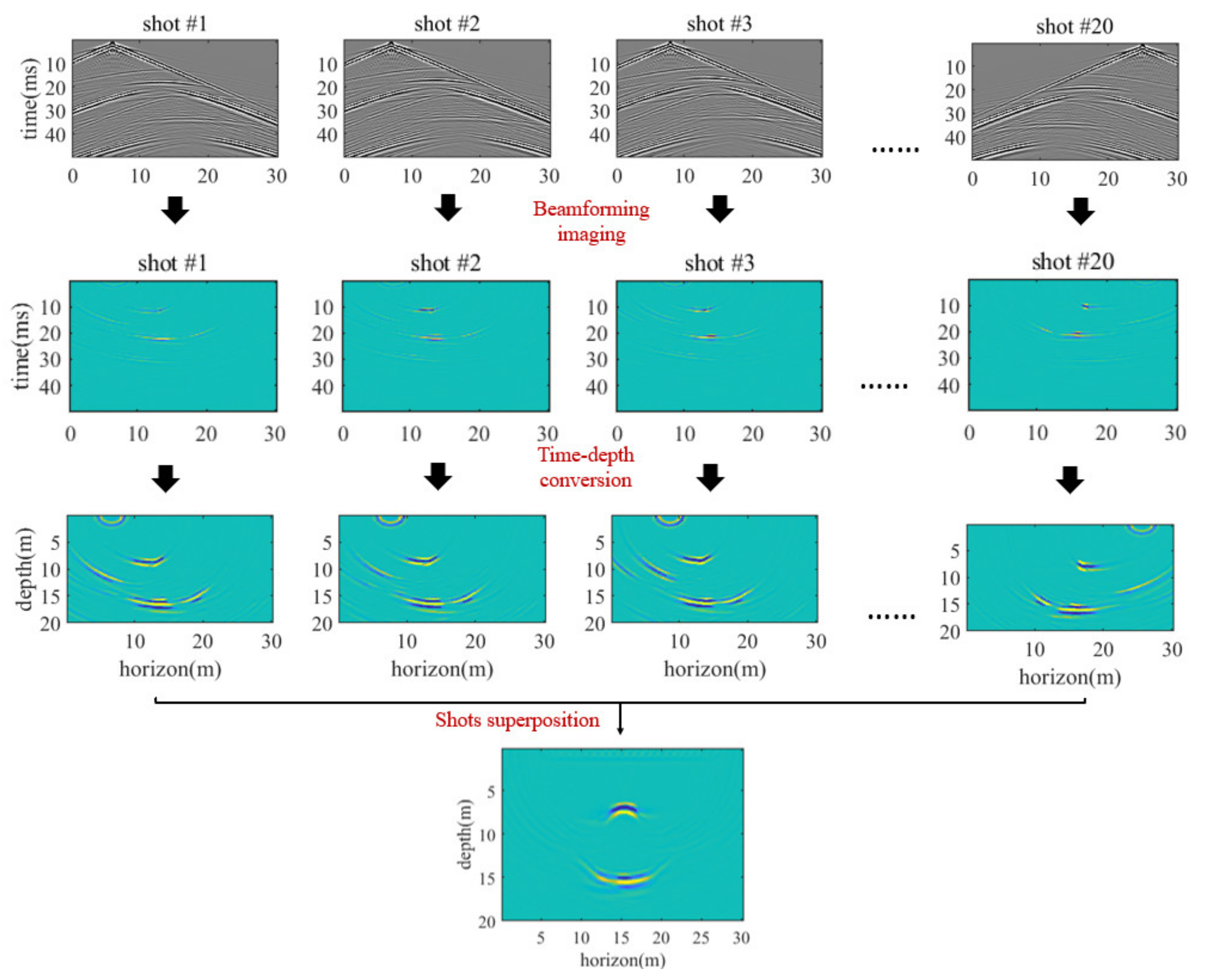
2. Methods
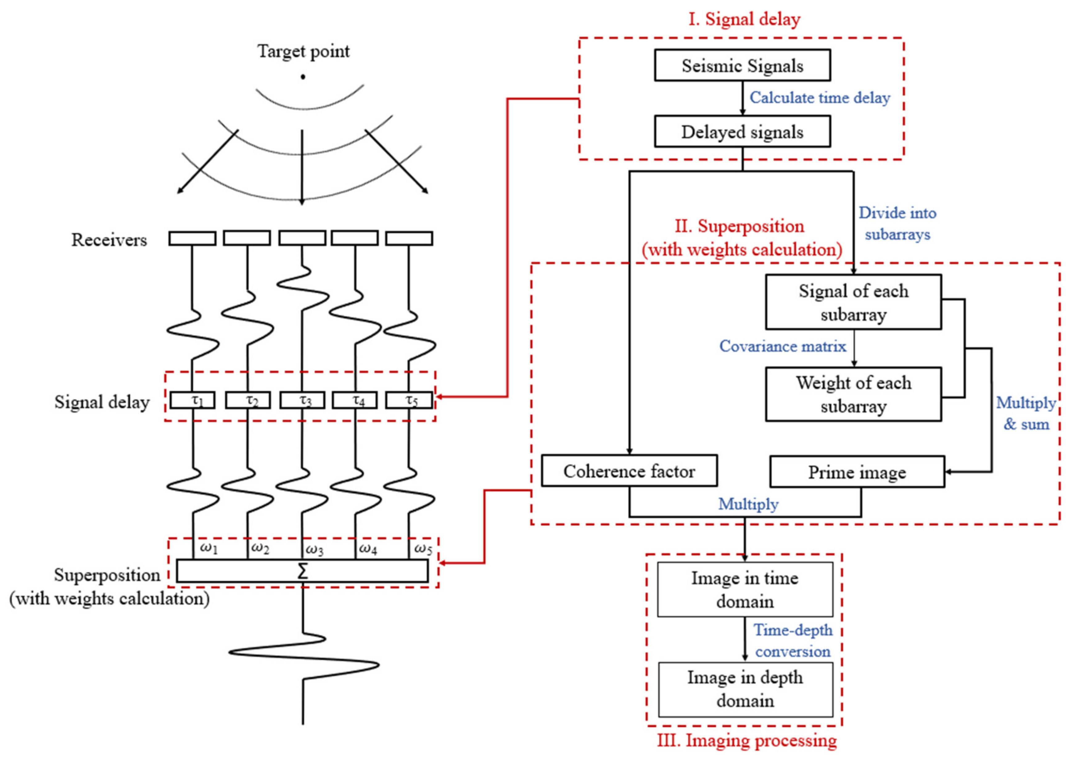
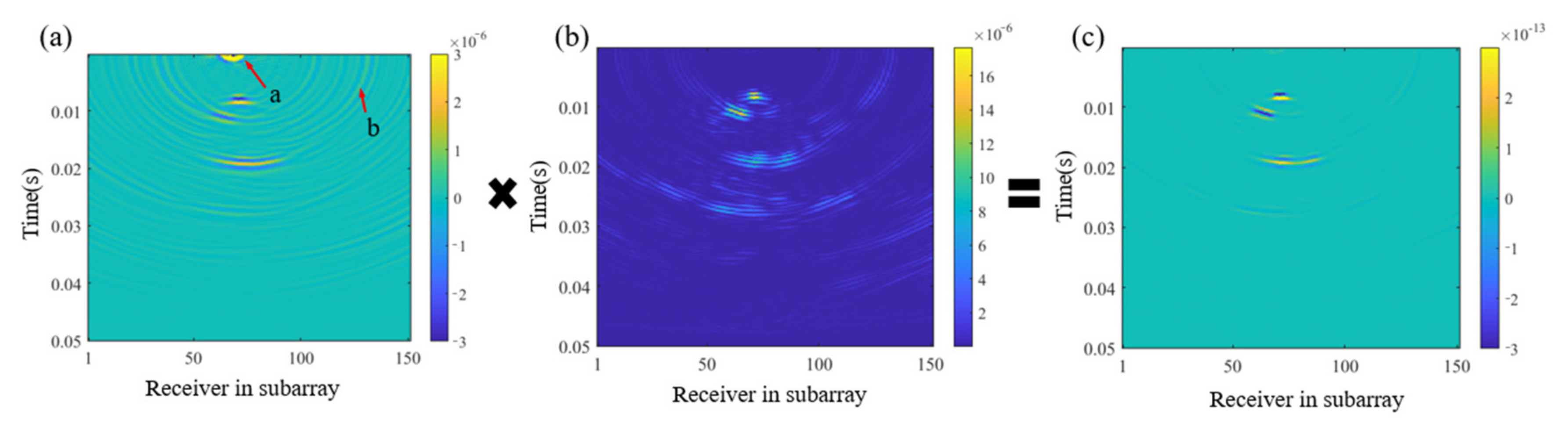
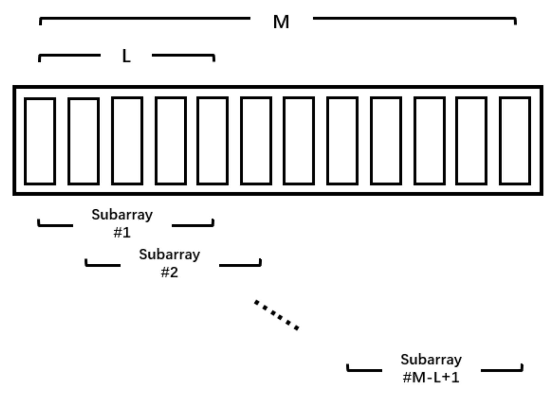
2.1. MVSS Beamforming Imaging
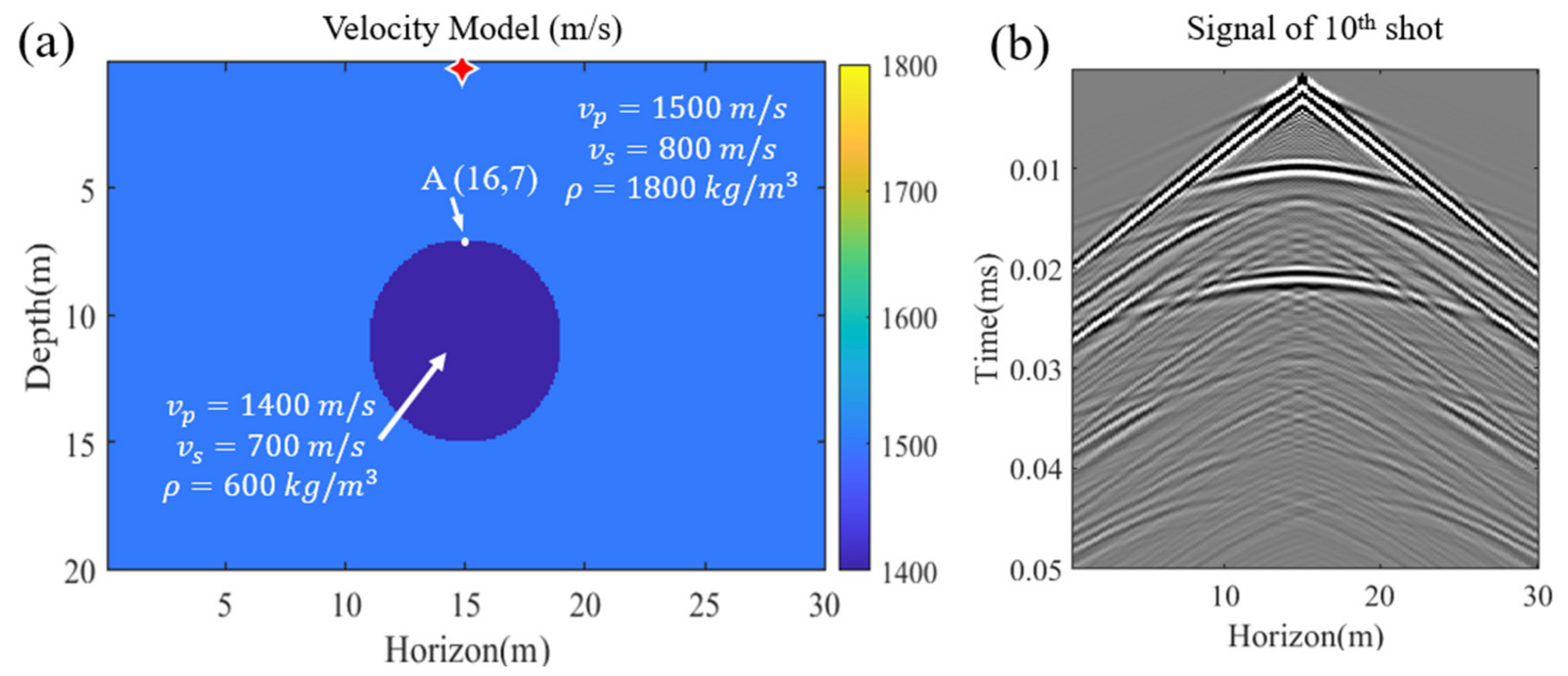
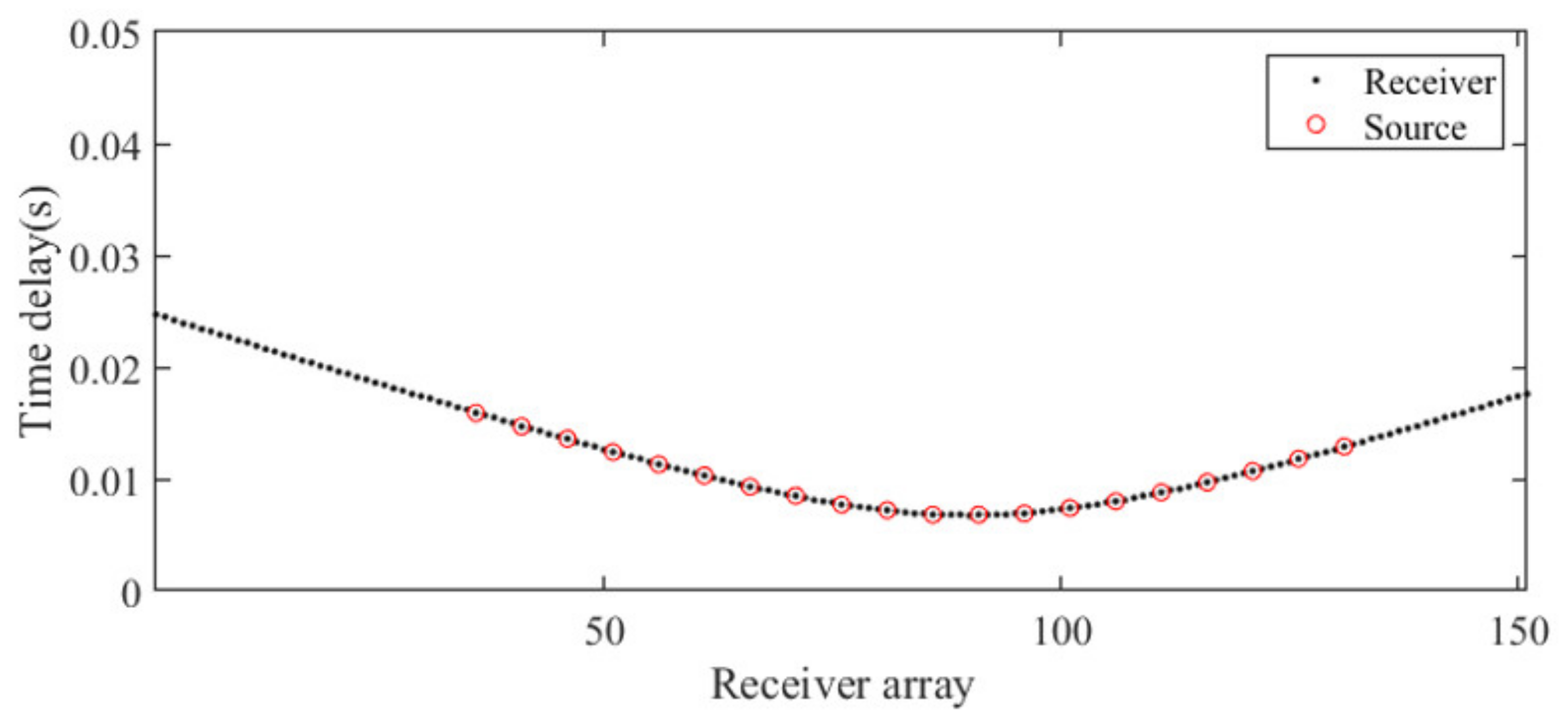
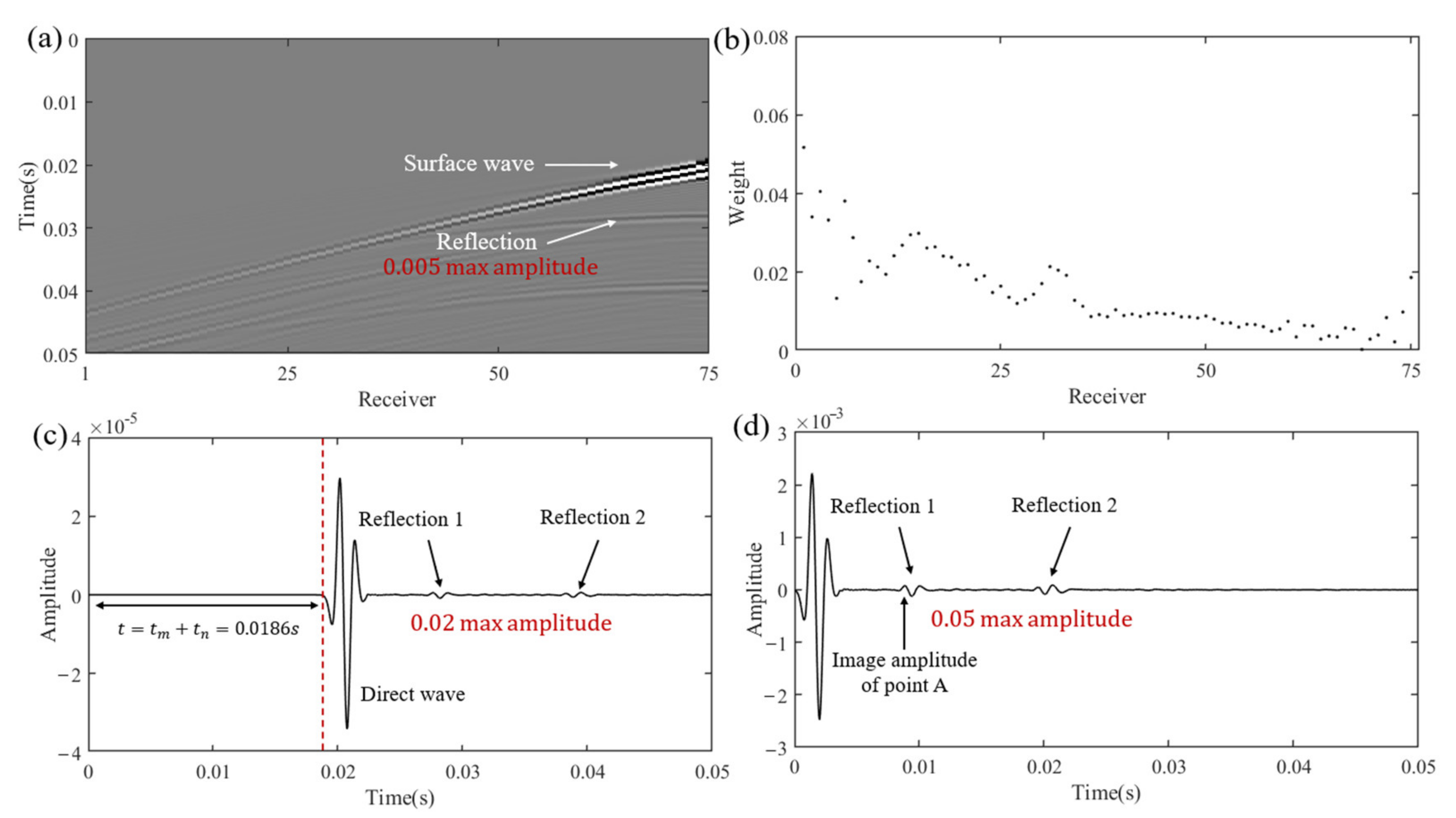
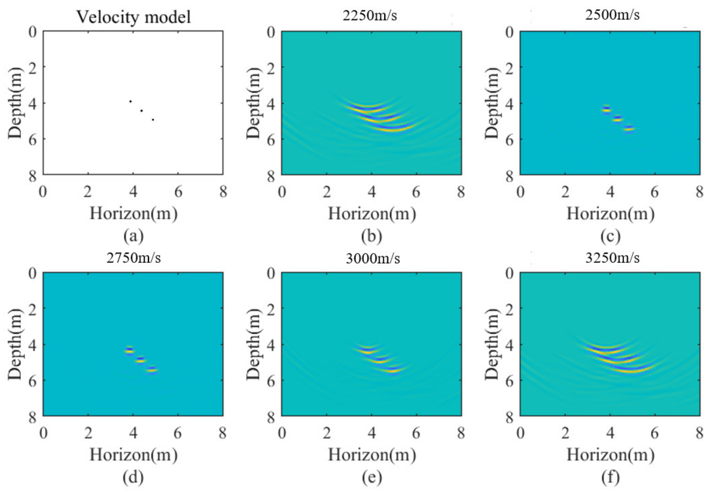
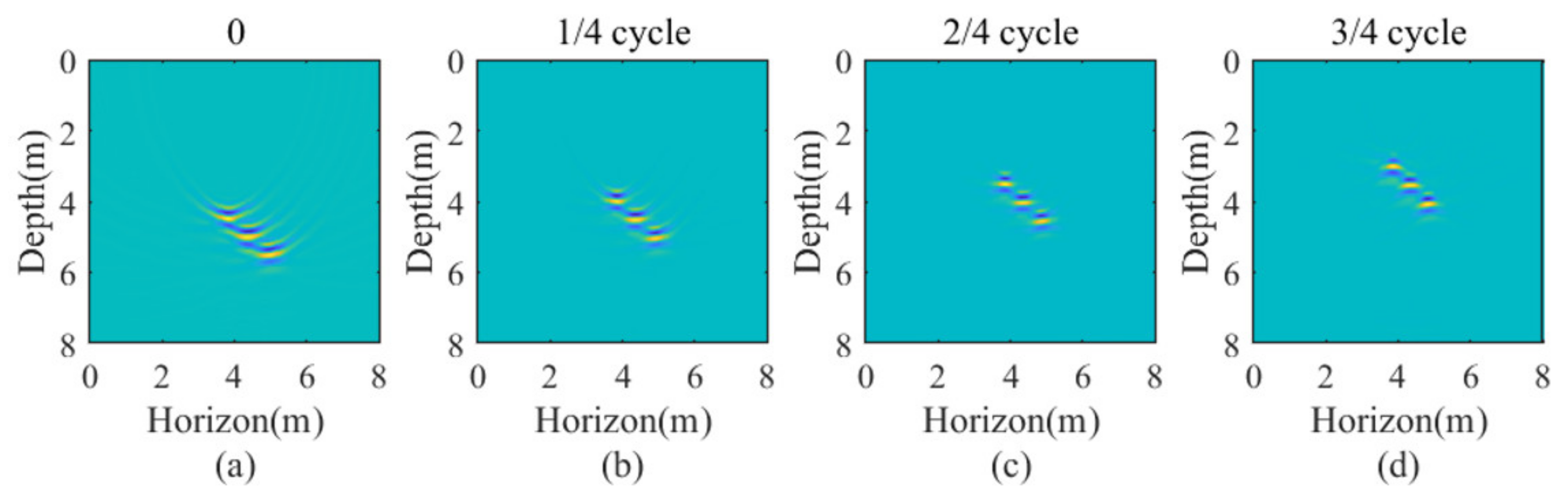
2.2. A Simple Example
2.3. Related Works
2.3.1. Kirchhoff Migration
2.3.2. Reverse Time Migration
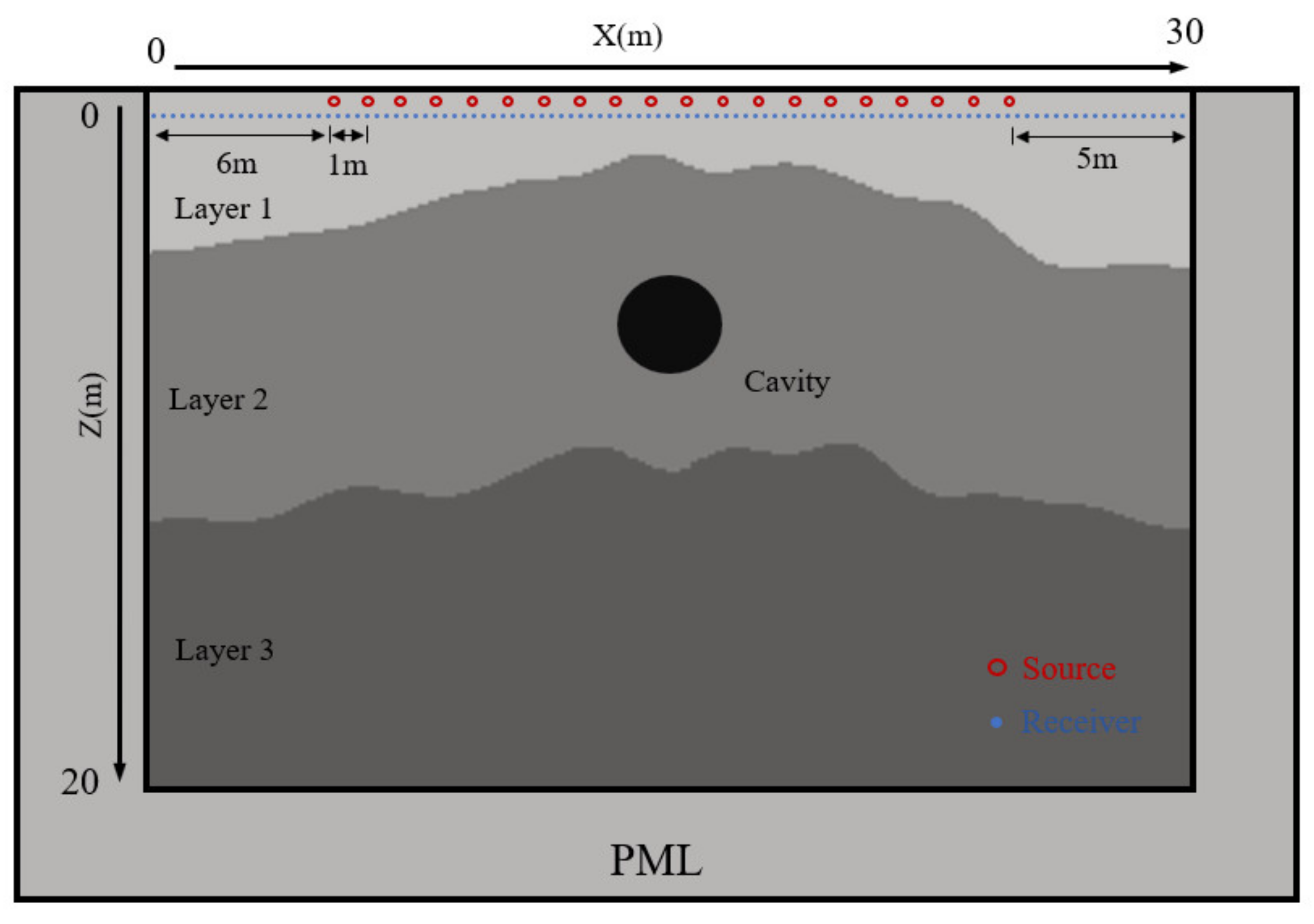
3. Numerical Experiments
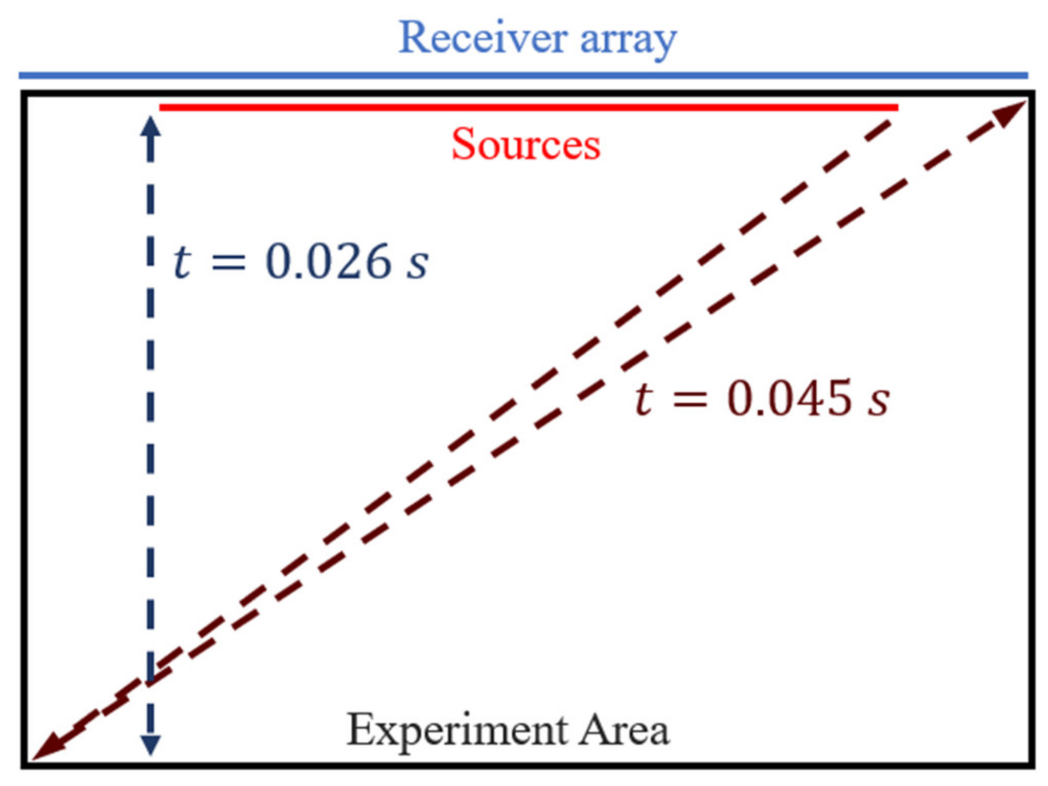
3.1. Numerical Experiments
3.2. Imaging Results
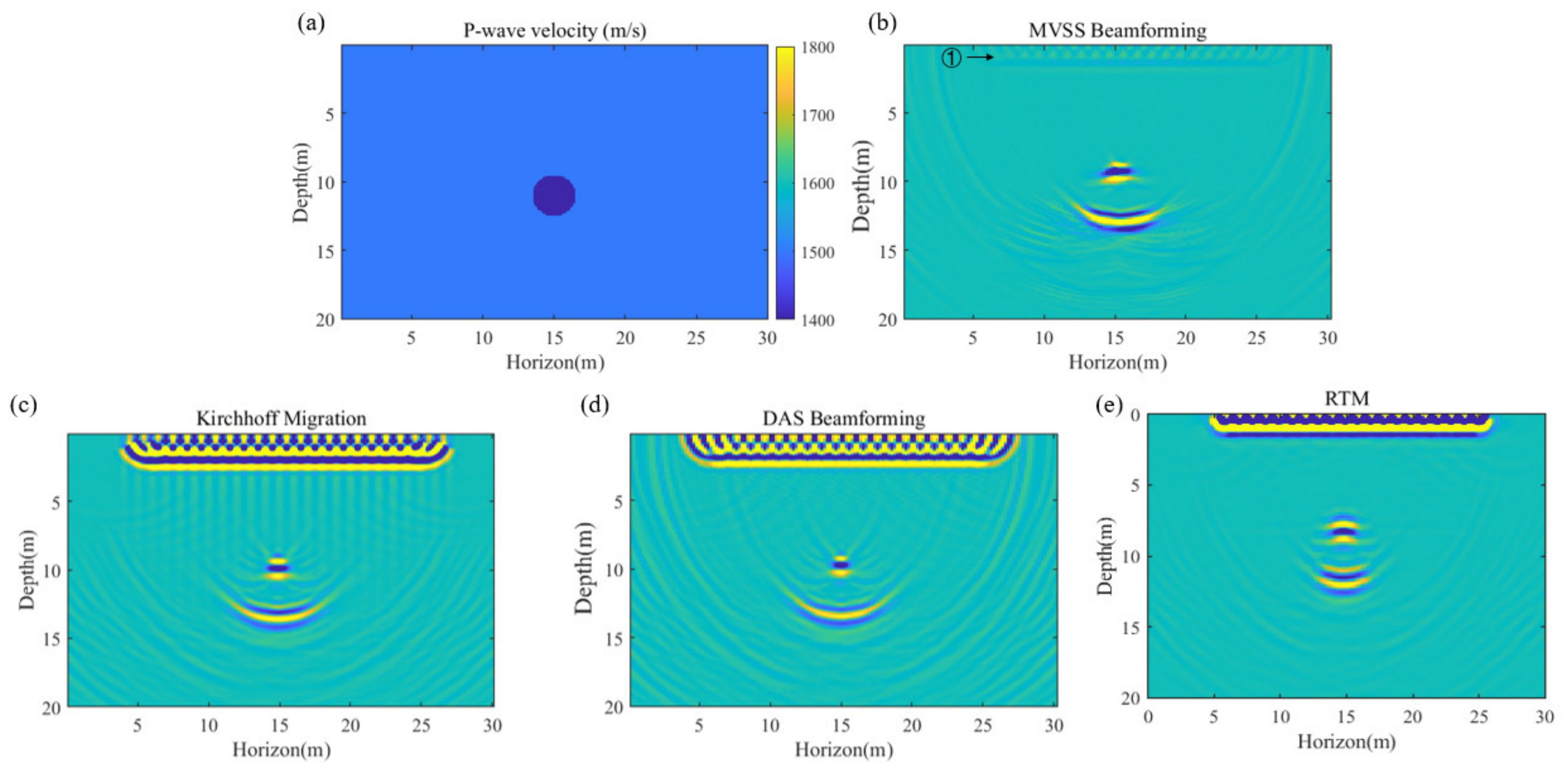
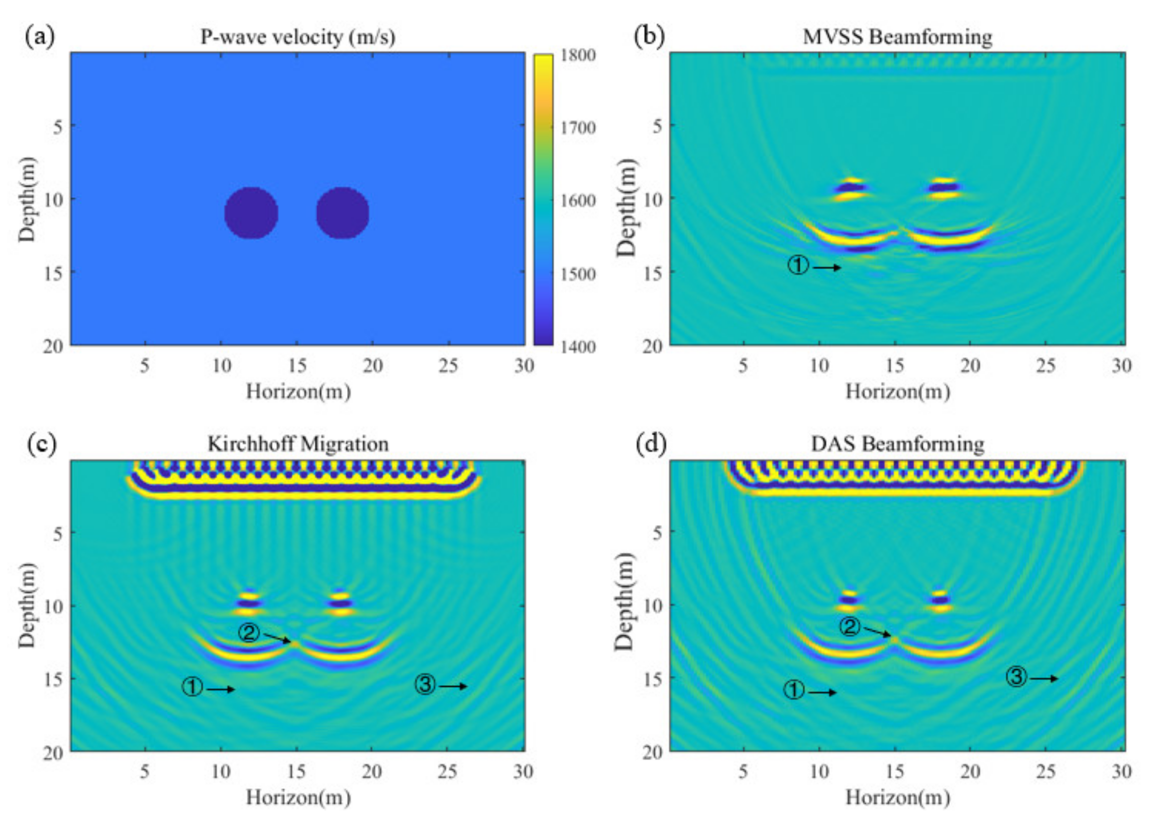
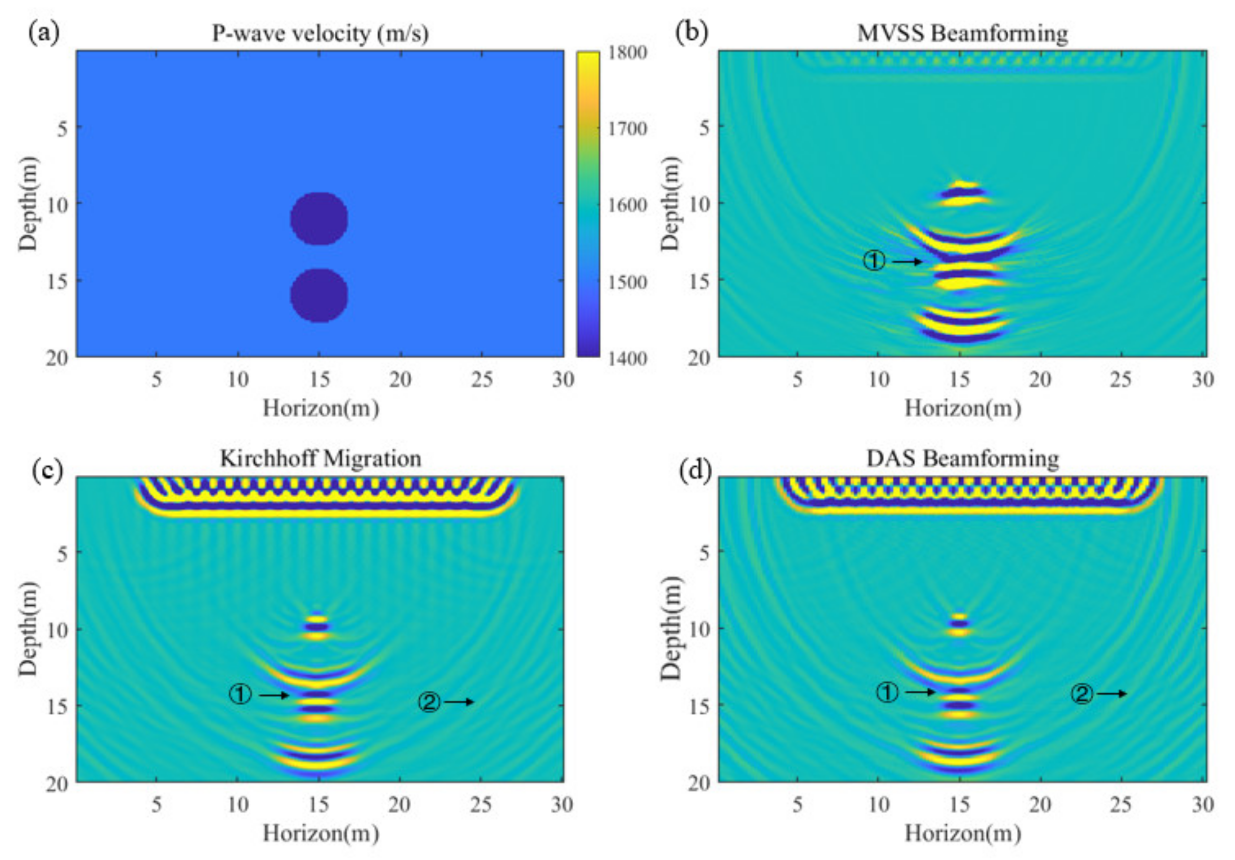
3.2.1. Cave Models
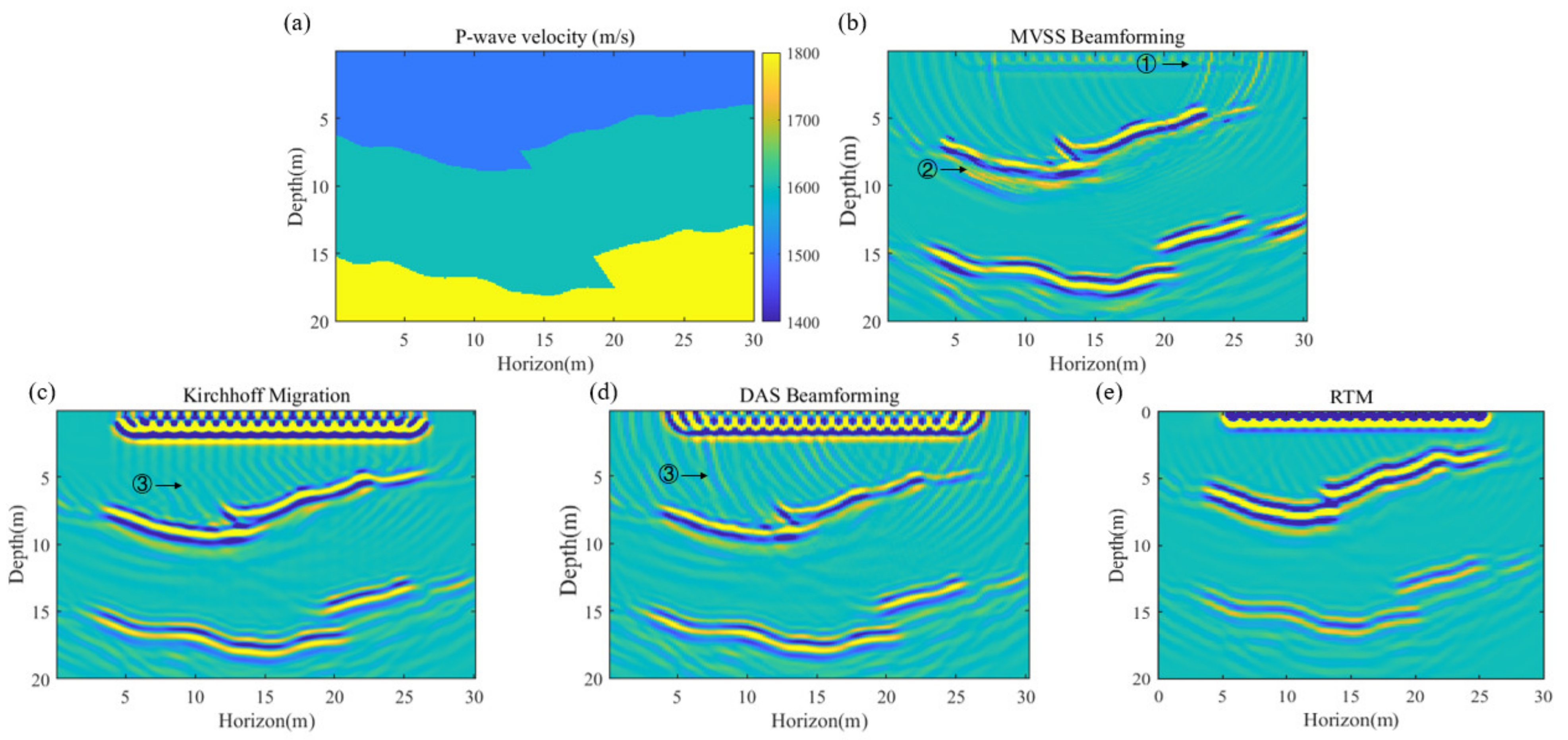
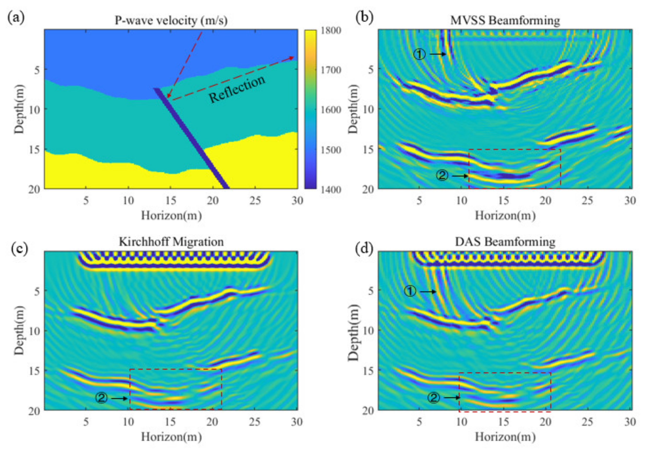
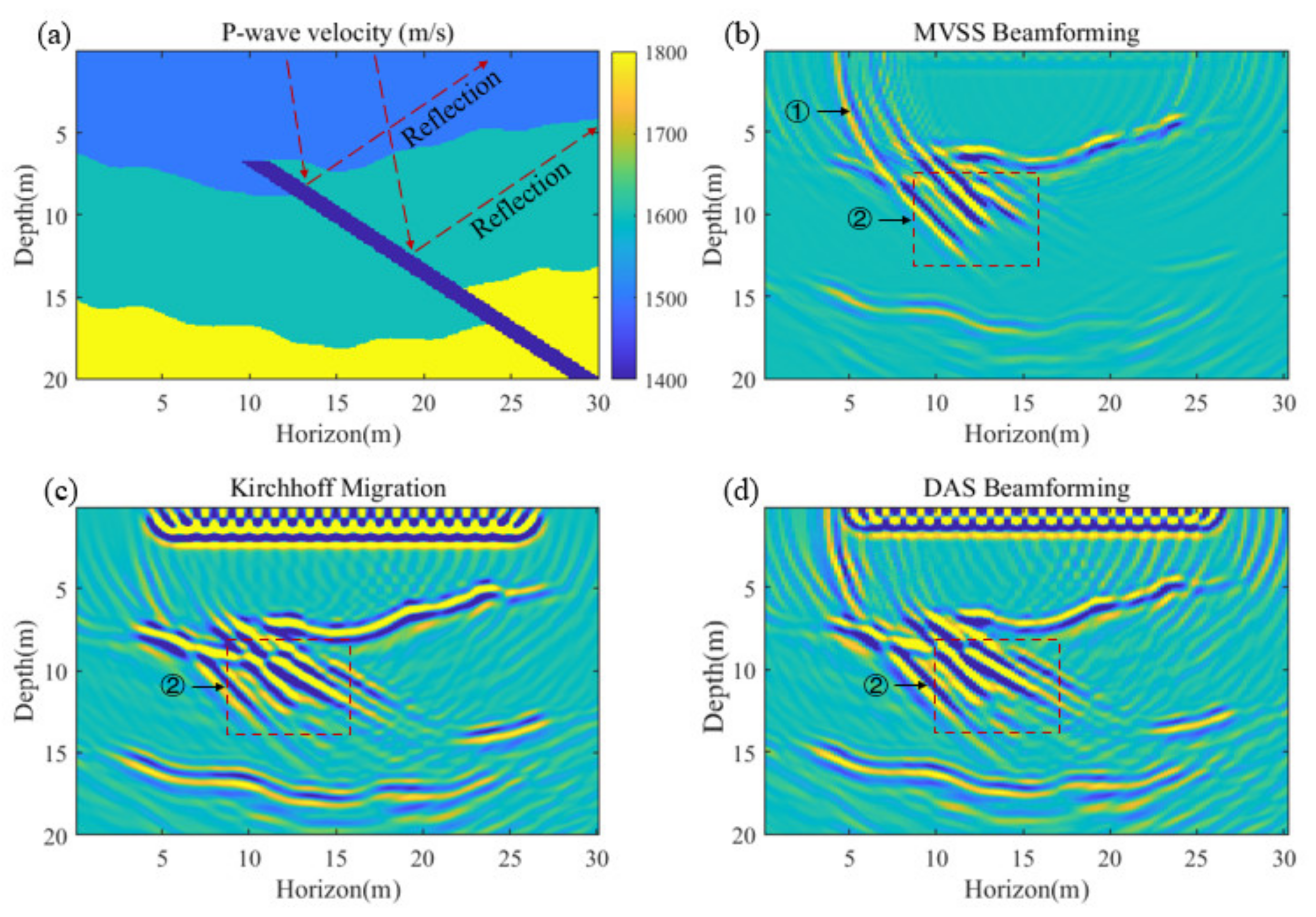
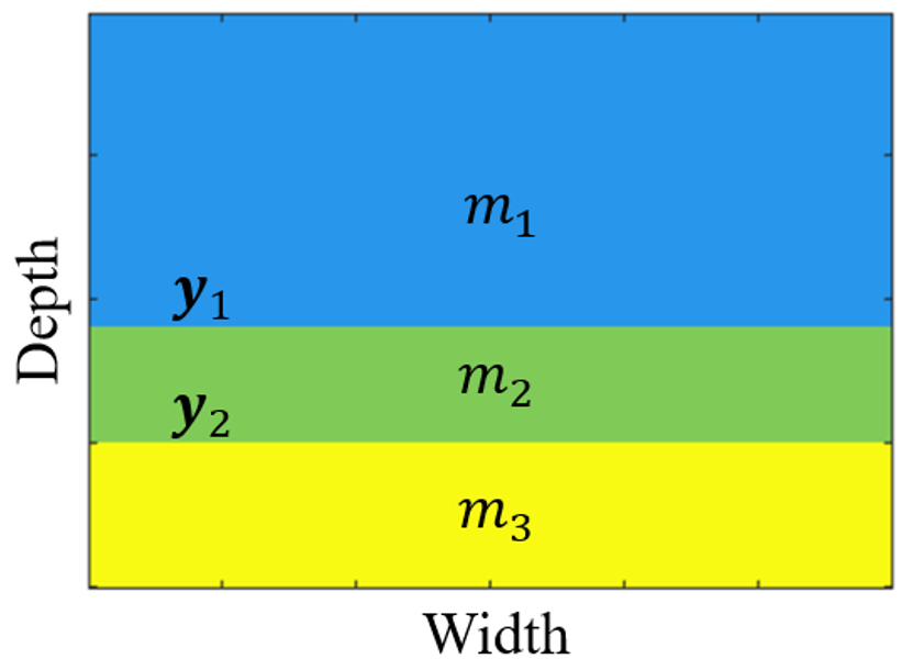
3.2.2. Layer Models
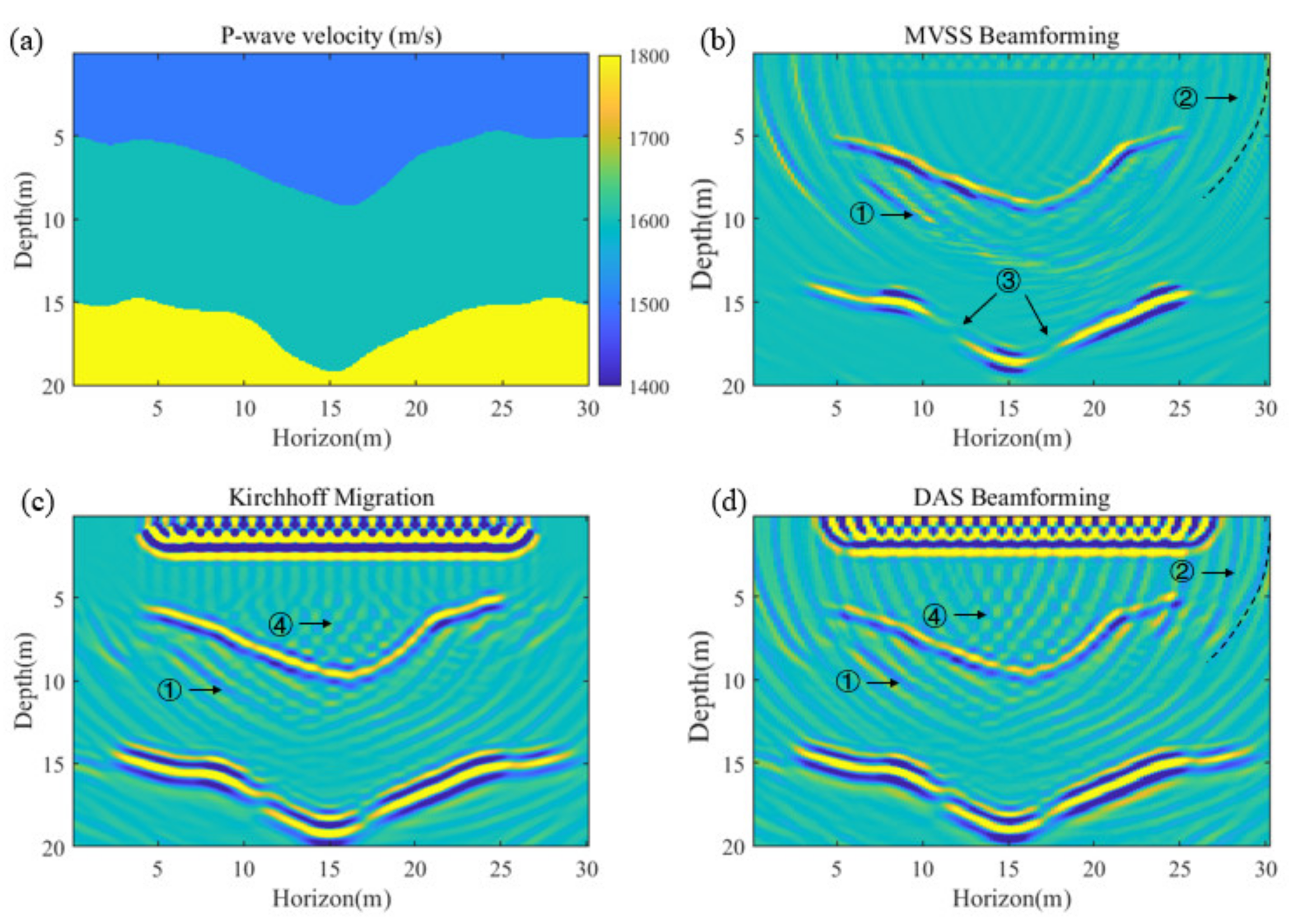
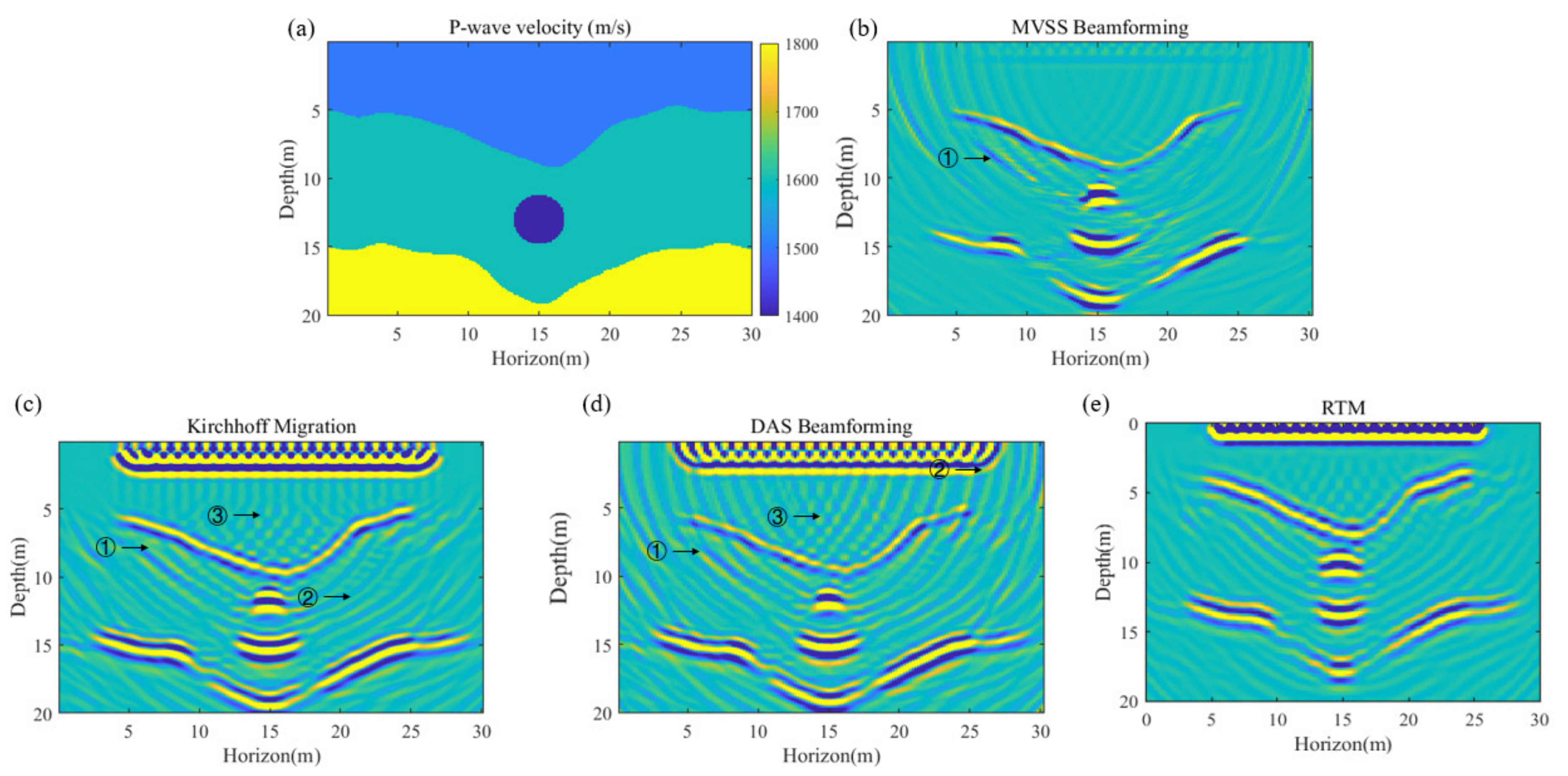
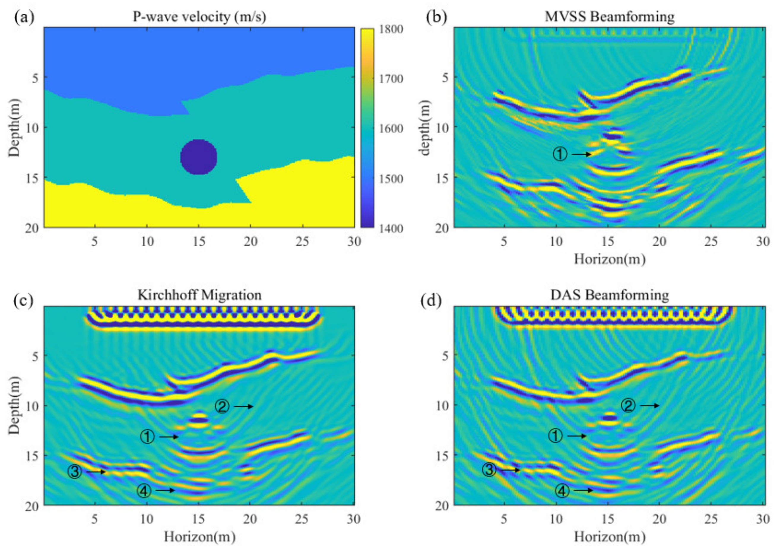
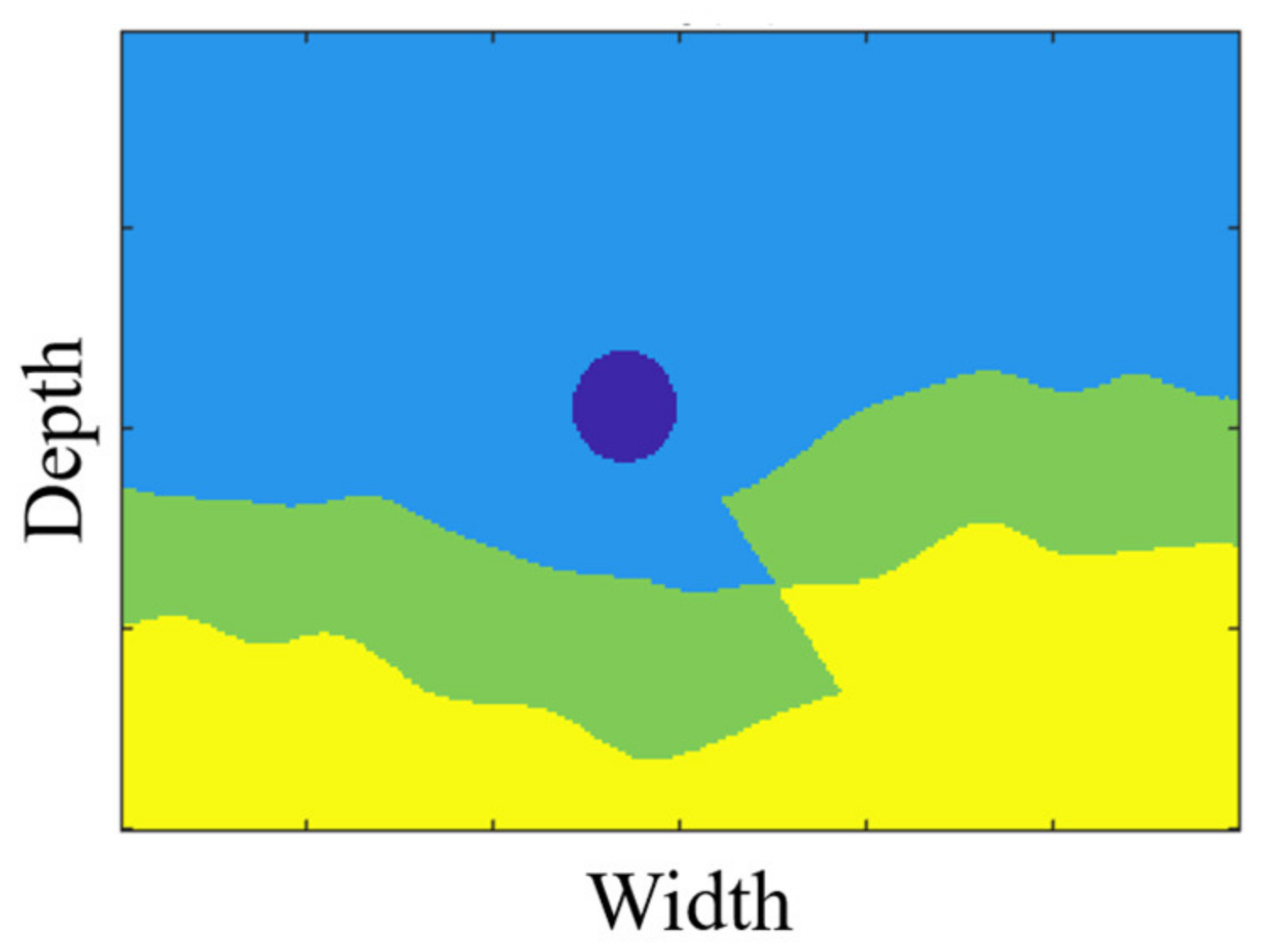
3.2.3. Cave-Layer Hybrid Models
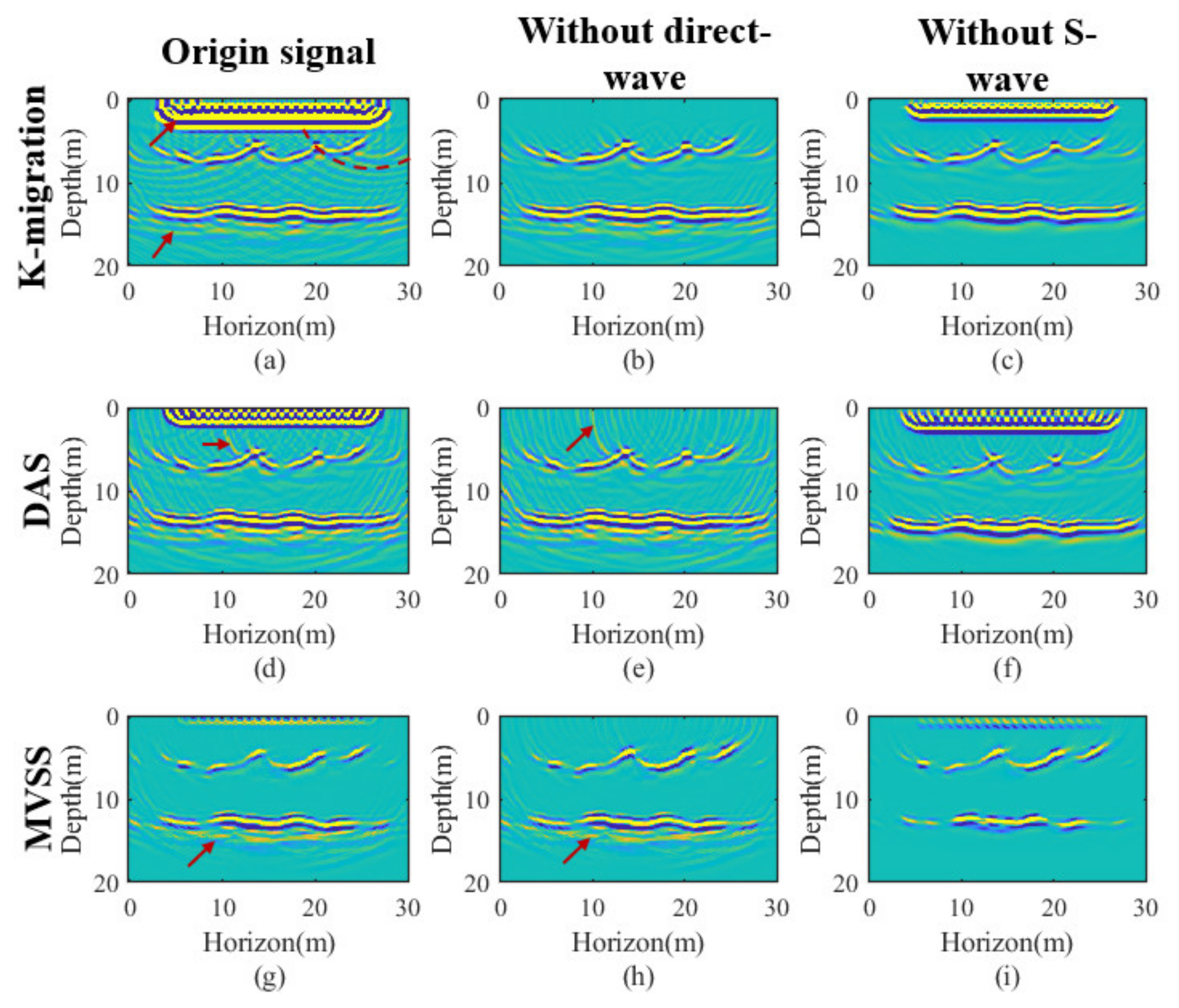
3.3. Robustness to Other Wave Components
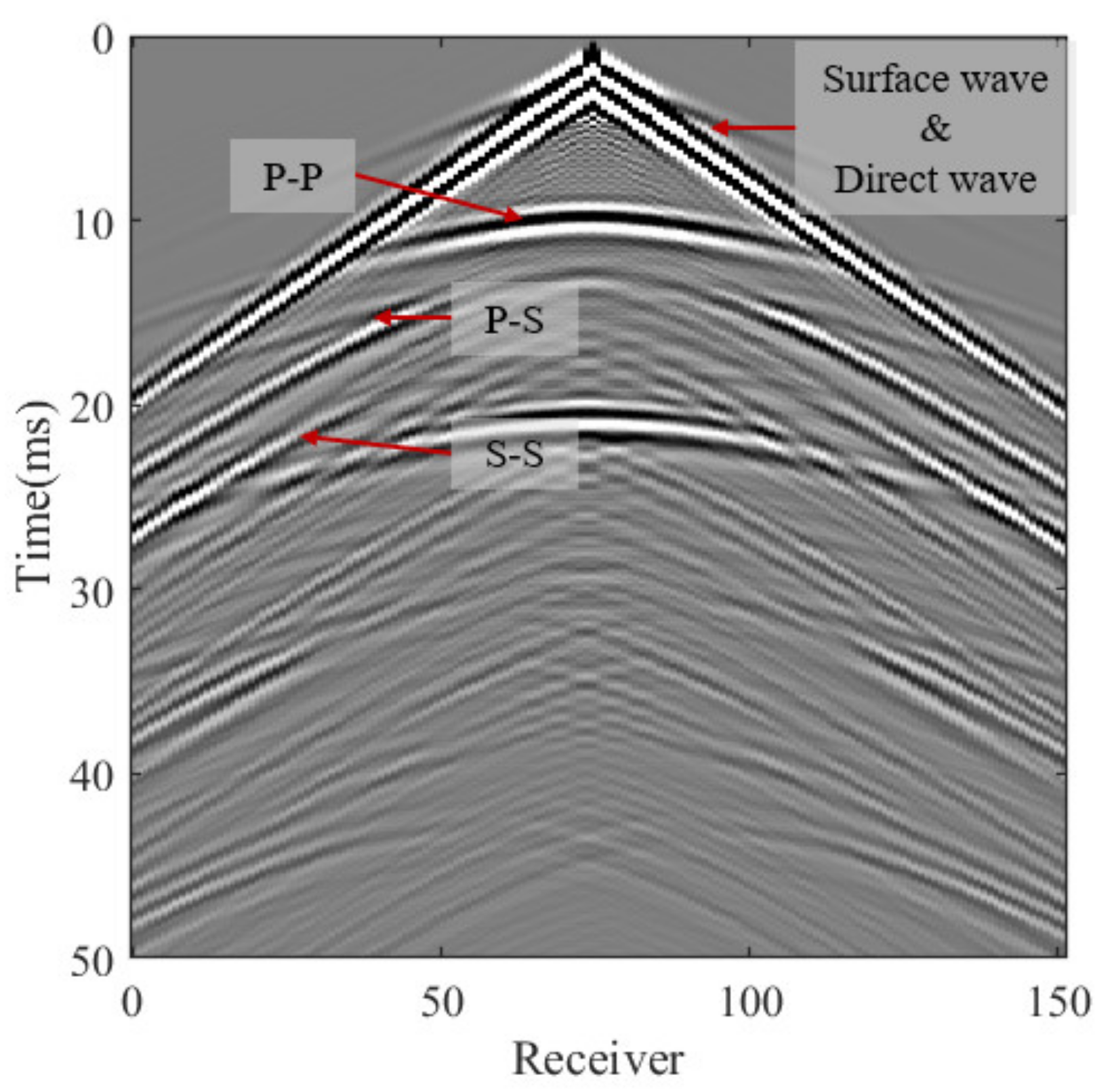
- The horizontal artifacts at the top of the images are caused by surface waves, while the artifacts beneath the interfaces are caused by S-waves, probably P-S waves;
- When S-waves are eliminated, the direct wave still exists, but the surface wave does not. This greatly weakens the artifacts at the top of the image;
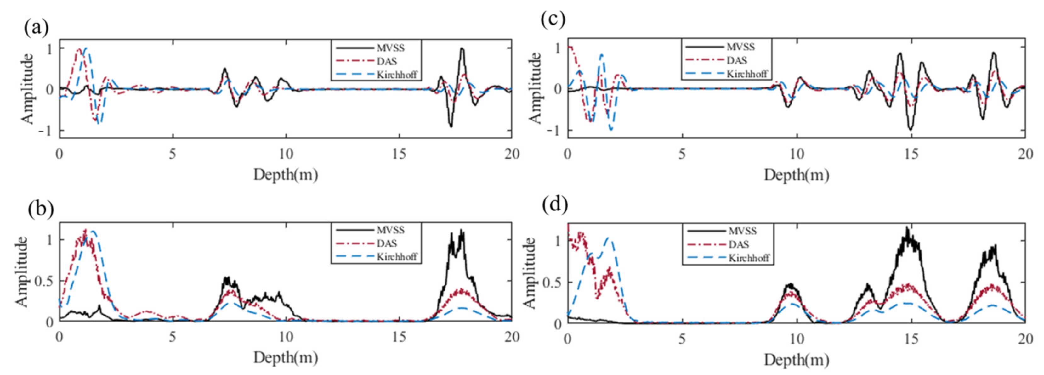
- The ability of MVSS beamforming to suppress surface wave artifacts at the top of the image and the S-wave artifacts on both sides of the interfaces is superior. However, the S-wave artifacts beneath the interfaces still affect MVSS beamforming as much as they do the other methods.
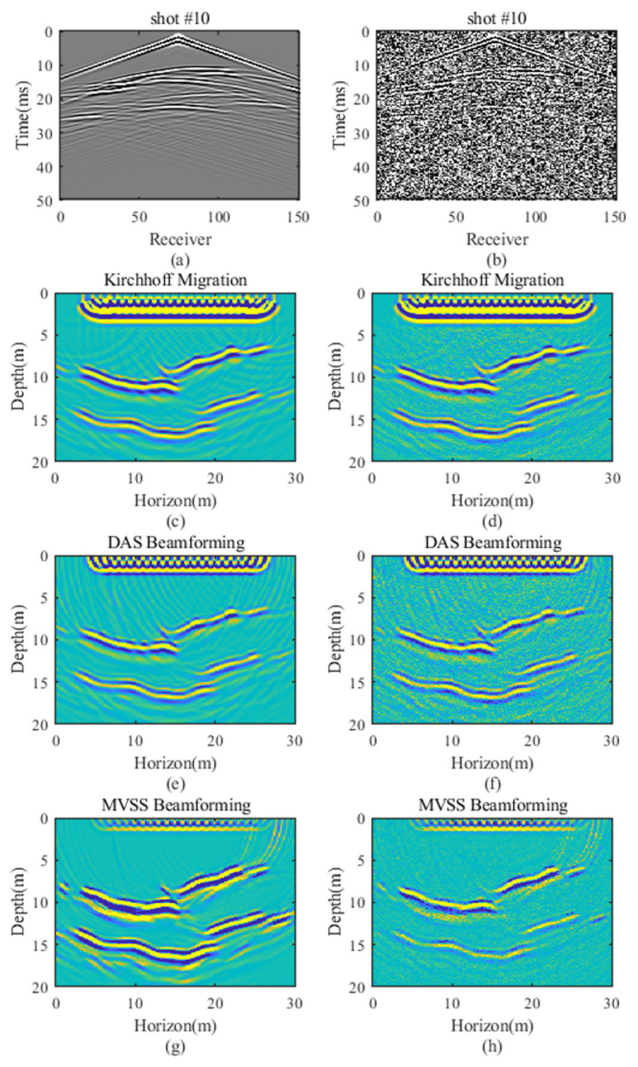
3.4. Robustness to Random Noise
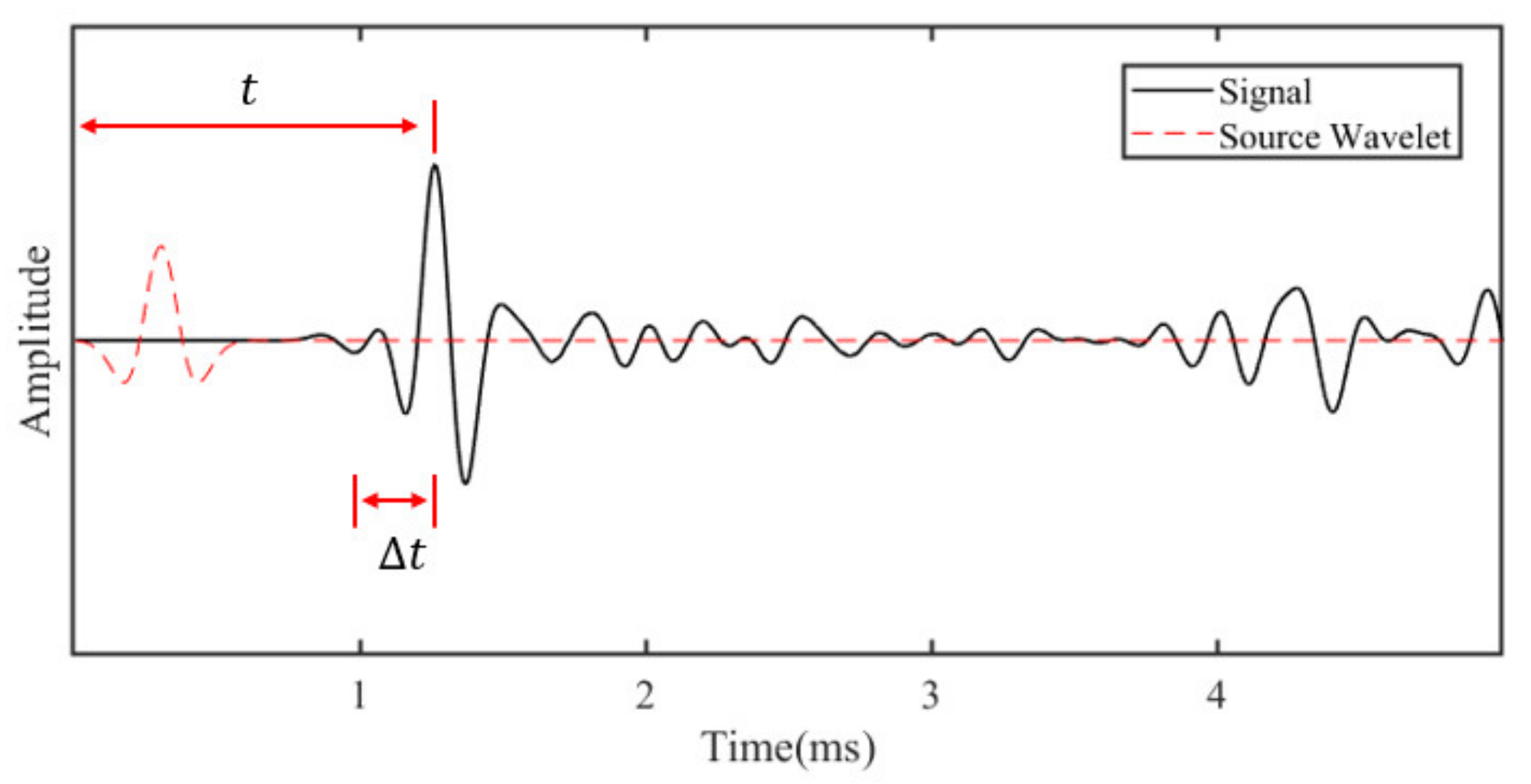
3.5. Focus Enhancing by a Signal Advance Correction
4. Discussion
4.1. Computational Efficiency
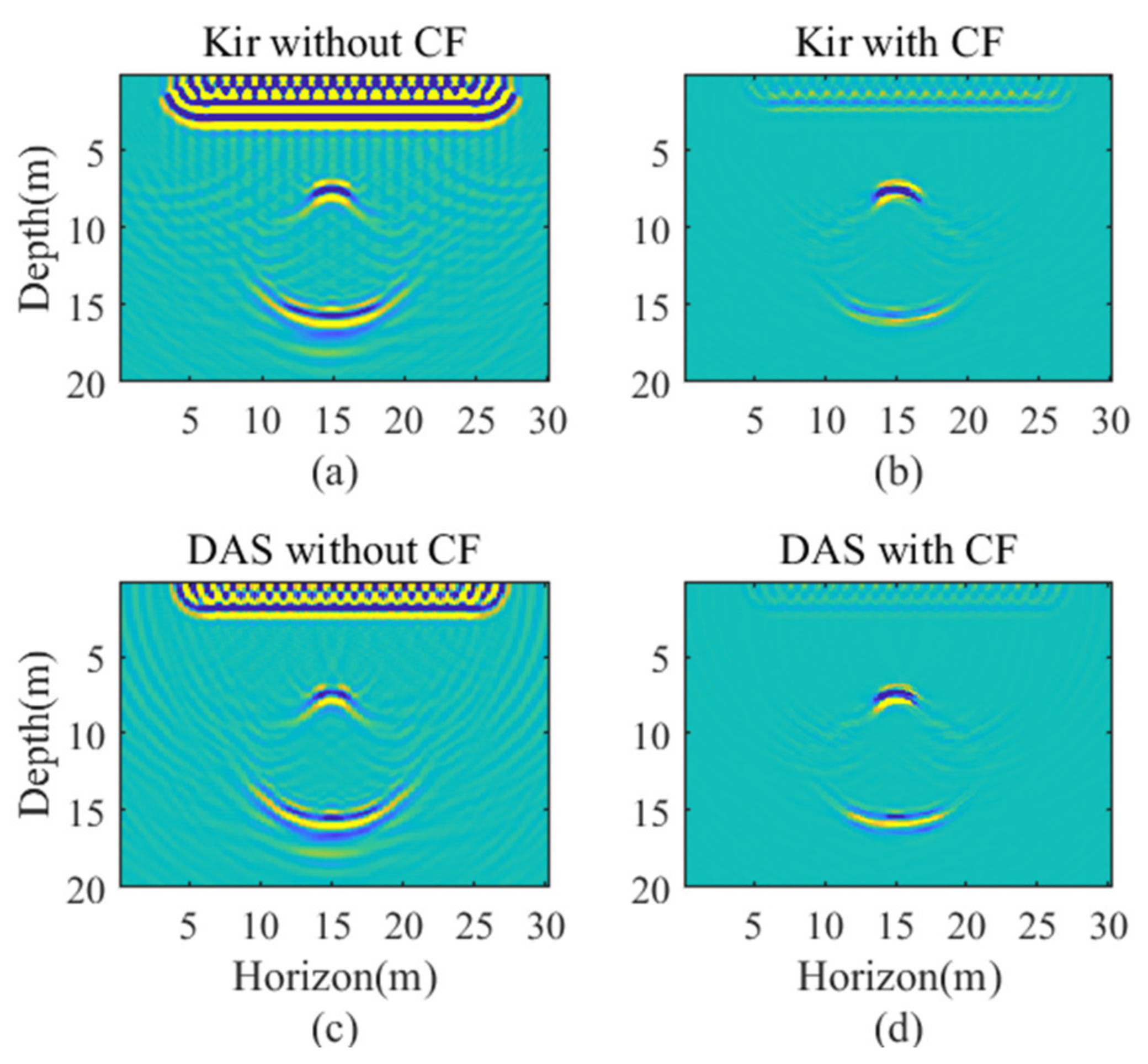
4.2. Coherence Factor Matrix
5. Conclusions
Author Contributions
Funding
Institutional Review Board Statement
Informed Consent Statement
Data Availability Statement
Conflicts of Interest
Appendix A. MVSS Beamforming Methodology
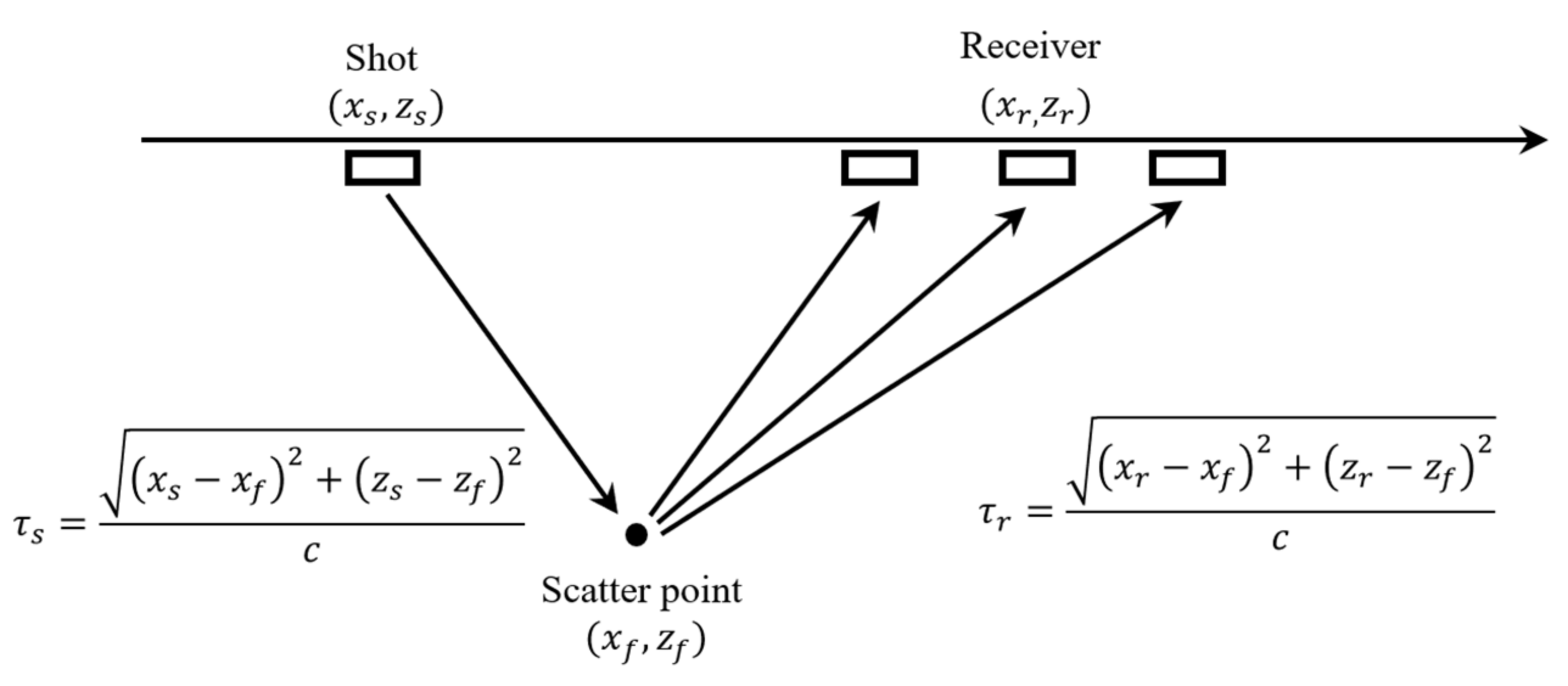
Appendix A.1. Signal Time Delay Calculation

Appendix A.2. Superposition with Weight Calculation

Appendix A.3. Image Processing and Stacking
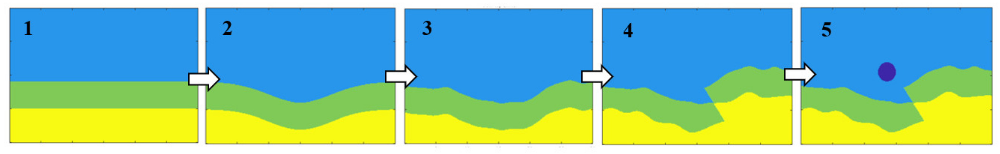
Appendix B. Near-Surface Model Generation Method
Appendix B.1. Horizontal Layer Model

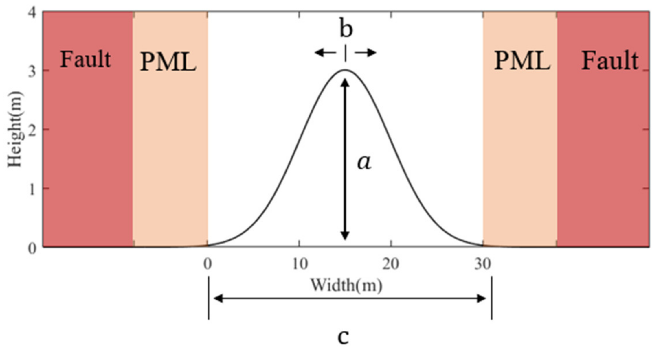
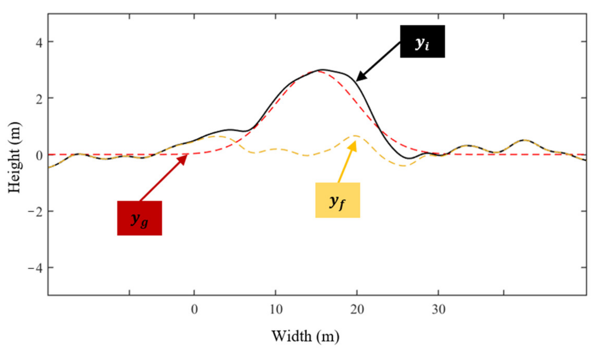
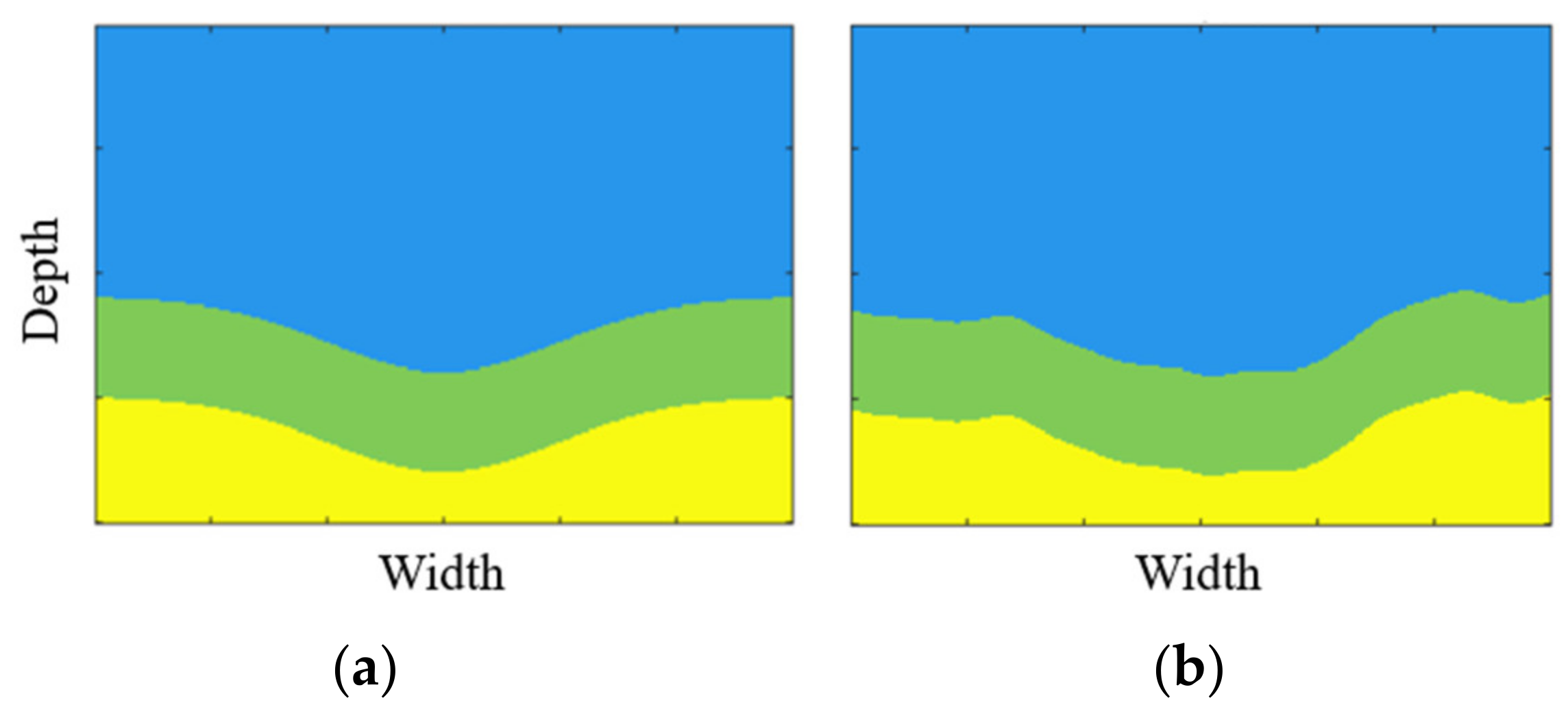
Appendix B.2. Fold


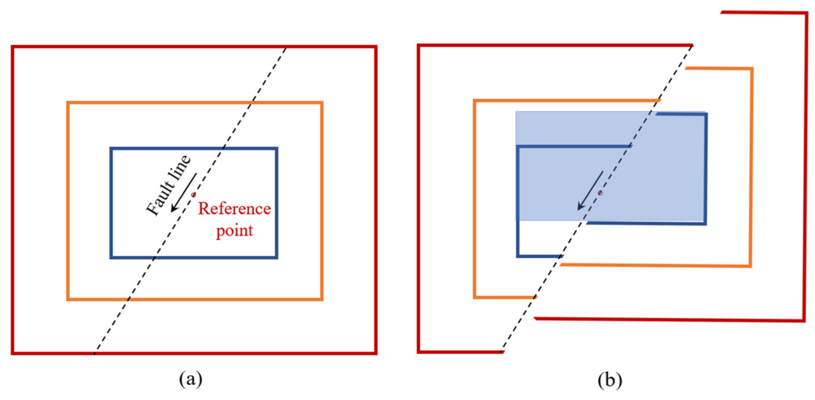
Appendix B.3. Fault

Appendix B.4. Cave

References
- Li, L.; Lei, T.; Li, S.; Zhang, Q.; Xu, Z.; Shi, S.; Zhou, Z. Risk assessment of water inrush in karst tunnels and software development. Arab. J. Geosci. 2014, 8, 1843–1854. [Google Scholar] [CrossRef]
- Xue, Y.; Li, S.; Ding, W.; Fang, C. Risk Evaluation System for the Impacts of a Concealed Karst Cave on Tunnel Construction. Mod. Tunn. Technol. 2017, 54, 41–47. [Google Scholar]
- Lei, M.; Gao, Y.; Jiang, X. Current Status and Strategic Planning of Sinkhole Collapses in China. In Engineering Geology for Society and Territory; Springer: Berlin/Heidelberg, Germany, 2015; Volume 5, pp. 529–533. [Google Scholar]
- Gutiérrez, F.; Parise, M.; de Waele, J.; Jourde, H. A review on natural and human-induced geohazards and impacts in karst. Earth Sci. Rev. 2014, 138, 61–88. [Google Scholar] [CrossRef]
- Li, X.; Dou, S.E.; Qu, H. A View on Application and Development of Engineering Geophysical Prospecting and Testing in City. Chin. J. Eng. Geophys. 2008, 05, 564–573. [Google Scholar]
- Bakulin, A.; Silvestrov, I.; Dmitriev, M.; Neklyudov, D.; Protasov, M.; Gadylshin, K.; Dolgov, V. Nonlinear Beamforming for Enhancement of 3D Prestack Land Seismic Data. Geophysics 2020, 85, 283–296. [Google Scholar] [CrossRef]
- Zhang, J.; Liu, S.; Yang, C.; Liu, X.; Wang, B. Detection of urban underground cavities using seismic scattered waves: A case study along the Xuzhou Metro Line 1 in China. Near Surf. Geophys. 2020, 19, 95–107. [Google Scholar] [CrossRef]
- Bednar, J.B. A brief history of seismic migration. Geophysics 2005, 70, 3MJ–20MJ. [Google Scholar] [CrossRef] [Green Version]
- Baysal, E.; Kosloff, D.D.; Sherwood, J.W.C. Reverse time migration. Geophysics 1983, 48, 1514–1524. [Google Scholar] [CrossRef] [Green Version]
- Xue, Z.G.; Chen, Y.K.; Fomel, S.; Sun, J.Z. Seismic imaging of incomplete data and simultaneous-source data using least-squares reverse time migration with shaping regularization. Geophysics 2016, 81, S11–S20. [Google Scholar] [CrossRef]
- Hill, N.R. Gaussian-Beam Migration. Geophysics 1990, 55, 1416–1428. [Google Scholar] [CrossRef]
- Hill, N.R. Prestack Gaussian-beam depth migration. Geophysics 2001, 66, 1240–1250. [Google Scholar] [CrossRef]
- Yang, F.; Sun, H. Application of Gaussian beam migration to VSP imaging. Acta Geophys. 2019, 67, 1579–1586. [Google Scholar] [CrossRef] [Green Version]
- Vidale, J. Finite-difference calculation of travel times. Bull. Seismol. Soc. Am. 1988, 78, 2062–2076. [Google Scholar]
- Zhang, K.; Cheng, J.B.; Ma, Z.T.; Zhang, W. Pre-stack time migration and velocity analysis methods with common scatter-point gathers. J. Geophys. Eng. 2006, 3, 283–289. [Google Scholar] [CrossRef]
- Yuan, Y.; Gao, Y.; Bai, L.; Liu, Z. Prestack Kirchhoff time migration of 3D coal seismic data from mining zones. Geophys. Prospect. 2011, 59, 455–463. [Google Scholar] [CrossRef]
- Wang, Y.; Xu, J.; Xie, S.; Zhang, L.; Du, X.; Chang, X. Seismic imaging of subsurface structure using tomographic migration velocity analysis: A case study of South China Sea data. Mar. Geophys. Res. 2015, 36, 127–137. [Google Scholar] [CrossRef]
- Liu, Q.; Zhang, J. Trace-imposed stretch correction in Kirchhoff prestack time migration. Geophys. Prospect. 2018, 66, 1643–1652. [Google Scholar] [CrossRef]
- Havlice, J.F.; Taenzer, J.C. Medical ultrasonic imaging: An overview of principles and instrumentation. Proc. IEEE 1979, 67, 620–641. [Google Scholar] [CrossRef]
- Kollmann, C. Diagnostic Ultrasound Imaging: Inside Out (Second Edition). Ultrasound Med. Biol. 2015, 41, 622. [Google Scholar] [CrossRef]
- Capon, J. High-resolution frequency-wavenumber spectrum analysis. Proc. IEEE 1969, 57, 1408–1418. [Google Scholar] [CrossRef] [Green Version]
- Tie-Jun, S.; Kailath, T. Adaptive beamforming for coherent signals and interference. IEEE Trans. Acoust. Speech Signal Process. 1985, 33, 527–536. [Google Scholar] [CrossRef] [Green Version]
- Mann, J.A.; Walker, W.F. A constrained adaptive beamformer for medical ultrasound: Initial results. In Proceedings of the IEEE International Ultrasonic Symposium, Munich, Germany, 8–11 October 2002; pp. 1807–1810. [Google Scholar]
- Sasso, M.; Cohen-Bacrie, C. Medical ultrasound imaging using the fully adaptive beamformer. In Proceedings of the IEEE International Conference on Acoustics, Speech, and Signal, Philadelphia, PA, USA, 18–23 March 2005. [Google Scholar]
- Synnevag, J.F.; Austeng, A.; Holm, S. Adaptive Beamforming Applied to Medical Ultrasound Imaging. IEEE Trans. Ultrason. Ferroelectr. Freq. Control. 2007, 54, 1606–1613. [Google Scholar] [CrossRef] [Green Version]
- Asl, B.M.; Mahloojifar, A. Minimum Variance Beamforming Combined with Adaptive Coherence Weighting Applied to Medical Ultrasound Imaging. IEEE Trans. Ultrason. Ferroelectr. Freq. Control. 2009, 56, 1923–1931. [Google Scholar] [CrossRef]
- Ma, X.; Peng, C.; Yuan, J.; Cheng, Q.; Xu, G.; Wang, X.; Carson, P.L. Multiple Delay and Sum with Enveloping Beamforming Algorithm for Photoacoustic Imaging. IEEE Trans. Med. Imag. 2020, 39, 1812–1821. [Google Scholar] [CrossRef] [PubMed]
- Chen, J.; Chen, J.; Zhuang, R.; Min, H. Multi-Operator Minimum Variance Adaptive Beamforming Algorithms Accelerated with GPU. IEEE Trans. Med. Imag. 2020, 39, 2941–2953. [Google Scholar] [CrossRef]
- Liu, L.; Shi, Z.; Peng, M.; Liu, C.; Tao, F.; Liu, C. Numerical modeling for karst cavity sonar detection beneath bored cast in situ pile using 3D staggered grid finite difference method. Tunn. Undergr. Space Technol. 2018, 82, 50–65. [Google Scholar] [CrossRef]
- Margrave, G.F.; Lamoureux, M.P. Numerical Methods of Exploration Seismology: With Algorithms in MATLAB®; Cambridge University Press: Cambridge, UK, 2019. [Google Scholar]
- Graves, R.W. Simulating seismic wave propagation in 3D elastic media using staggered-grid finite differences. Bull. Ssmol. Soc. Am. 1996, 86, 1091–1106. [Google Scholar]
- Wang, D.-Y.; Ling, Y. Phase-shift- and phase-filtering-based surface-wave suppression method. Appl. Geophys. 2016, 13, 614–620. [Google Scholar] [CrossRef]
- Hudson, J.E. Introduction to Adaptive Arrays. Electron. Power 1981, 27, 491. [Google Scholar] [CrossRef]
- Ning, M.; Goh, J.T. Efficient method to determine diagonal loading value. In Proceedings of the 2003 IEEE International Conference on Acoustics, Speech, and Signal Processing, Hong Kong, China, 6–10 April 2003. [Google Scholar]


| Parameter | Value |
|---|---|
| Receiver spacing interval | m |
| Source frequency | Hz |
| Sampling frequency | Hz |
| Background P-wave velocity | m/s |
| Receiver array length | m |
| Number of receivers | |
| Signal length | s |
| Model | Geological Structure Type | Caves | Cave Center Location (m) (Horizontal, Vertical) | Cave Radius (m) | Map | Description |
|---|---|---|---|---|---|---|
| A-1 | - | 1 | 15, 11 | 1.8 |  | A circular homogeneous cavity. |
| A-2 | - | 2 | 13, 11 and 17, 11 | 1.8 |  | A model with two horizontally aligned caves. |
| A-3 | - | 2 | 15, 11 and 15, 16 | 1.8 |  | A model with two vertically aligned caves. |
| B-1 | Syncline fold | - | - | - |  | Syncline model with a fold depth of 4 m. |
| B-2 | Fault | - | - | - |  | Fault model with a dislocation of 2 m and a great angle (). |
| B-3 | Fault | - | - | - |  | Fault model with a great angle weak fault layer. |
| B-4 | Fault | - | - | - |  | Fault model with a small angle weak fault layer (). |
| C-1 | Syncline fold | 1 | 15, 11 | 1.8 |  | Syncline model composed of three layers with a cavity. |
| C-2 | Fault | 1 | 15, 11 | 1.8 |  | Fault model composed of three layers with a cavity. |
| Sequence | P-Wave Velocity (m/s) | S-Wave Velocity (m/s) | Density (kg/m3) |
|---|---|---|---|
| Cave 1 | 1400 | 700 | 1600 |
| Layer 1 | 1500 | 800 | 1800 |
| Layer 2 | 1600 | 900 | 2000 |
| Layer 3 | 1800 | 1000 | 2200 |
| Method | Kirchhoff Migration | DAS Beamforming | MVSS Beamforming |
|---|---|---|---|
| Calculation Time (s) | 520.1 | 3.9 | 201.1 |
Publisher’s Note: MDPI stays neutral with regard to jurisdictional claims in published maps and institutional affiliations. |
© 2021 by the authors. Licensee MDPI, Basel, Switzerland. This article is an open access article distributed under the terms and conditions of the Creative Commons Attribution (CC BY) license (https://creativecommons.org/licenses/by/4.0/).
Share and Cite
Peng, M.; Wang, D.; Liu, L.; Liu, C.; Shi, Z.; Ma, F.; Shen, J. Near-Surface Geological Structure Seismic Wave Imaging Using the Minimum Variance Spatial Smoothing Beamforming Method. Appl. Sci. 2021, 11, 10827. https://0-doi-org.brum.beds.ac.uk/10.3390/app112210827
Peng M, Wang D, Liu L, Liu C, Shi Z, Ma F, Shen J. Near-Surface Geological Structure Seismic Wave Imaging Using the Minimum Variance Spatial Smoothing Beamforming Method. Applied Sciences. 2021; 11(22):10827. https://0-doi-org.brum.beds.ac.uk/10.3390/app112210827
Chicago/Turabian StylePeng, Ming, Dengyi Wang, Liu Liu, Chengcheng Liu, Zhenming Shi, Fuan Ma, and Jian Shen. 2021. "Near-Surface Geological Structure Seismic Wave Imaging Using the Minimum Variance Spatial Smoothing Beamforming Method" Applied Sciences 11, no. 22: 10827. https://0-doi-org.brum.beds.ac.uk/10.3390/app112210827