Fuzzy Sliding Mode Control of Vehicle Magnetorheological Semi-Active Air Suspension

Abstract

In order to reduce vehicle vibration during driving conditions, a fuzzy sliding mode control strategy (FSMC) for semi-active air suspension based on the magnetorheological (MR) damper is proposed. The MR damper used in the semi-active air suspension system was tested and analyzed. Based on the experimental data, the genetic algorithm was used to identify the parameters of the improved hyperbolic tangent model, which was derived for the MR damper. At the same time, an adaptive neuro fuzzy inference system (ANFIS) was used to build the reverse model of the MR damper. The model of a quarter vehicle semi-active air suspension system equipped with a MR damper was established. Aiming at the uncertainty of the air suspension system, fuzzy control was used to adjust the boundary layer of the sliding mode control, which can effectively suppress the influence of chattering on the control accuracy and ensure system stability. Taking random road excitation and impact road excitation as the input signal, the simulation analysis of passive air suspension, semi-active air suspension based on SMC and FSMC was carried out, respectively. The results show that the semi-active air suspension based on FSMC has better vibration attenuating performance and ride comfort.

1. Introduction

The suspension system is the transmission device connecting the wheels and the car body, which mainly undertakes the body mass and ensures good contact between the tire and the ground, as well as reducing the uneven excitation from the road surface [1]. Compared with the traditional suspension system, the air spring suspension system has the advantages of being light weight, being low noise and having favorable vibration isolation performance. The air spring has the characteristics of non-linearity and self-adaptation, which makes the deviation frequency of the vehicle body mass in a stable state under the condition of load changes and obtains favorable ride comfort and handling stability [2,3,4,5].

As a new type of intelligent semi-active control device, the MR damper has become a research hotspot and can be well applied to semi-active air suspension, due to its good performance, i.e., simple structure, controllable damping force, low power consumption as well as rapid response time [6,7,8,9]. In industrial application, the accurate establishment of the mathematical model of MR damper is an important step for the design and analysis of the semi-active controller. However, the influences of movement condition of the piston, applied magnetic field, displacement amplitude and frequency on the dynamic performance of MR damper are inevitable, and the MR damper has the strong nonlinear characteristics, such as yield, hysteresis and saturation. It is difficult to establish the accurate dynamic model of the MR damper. So far, different mechanical models of MR damper have been proposed, which are mainly divided into two categories: non-parametric models and parametric models [10]. Parametric modeling of the MR damper is a process of replacing the mechanical behavior of the MR damper by the combination of a damping element, elastic element, mechanical element, etc. This type of model is relatively simple in structure, and there are many existing research studies, such as the Bingham model, Sigmoid model and hyperbolic tangent model, which are applied in semi-active control [11]. Non-parametric models, such as the differential equation model, neural network model and polynomial model, mainly simulate the mechanical properties of MR dampers by means of intelligent control [12]. However, these non-parametric models do not consider the rheological properties of MR fluid and have poor adaptability. Kowk et al. proposed the hyperbolic tangent model based on the study of the hyperbolic tangent function, which is mainly composed of three parallel structures of the hysteretic force element, damping element and spring element [13]. The hyperbolic tangent model can accurately describe the hysteretic characteristics of the MR damper by using the characteristics of the hyperbolic tangent function, but there are many parameters to be identified. Guo et al. constructed an improved hyperbolic tangent model, which applies another hyperbolic tangent function and is composed of viscous damping elements and elastic elements in series and parallel [14].

Appropriate control algorithms can make the semi-active air suspension almost achieve the same vibration attenuation effect as the active air suspension. In recent years, the sliding mode control (SMC) with strong anti-interference ability and good robustness attracted more and more attention in related fields. Choi et al. designed a sliding mode controller for the vehicle seat and considered the human body mass as the uncertainty factor of the system [15]. Through simulation analysis, it is concluded that the sliding mode controller has favorable robustness to the uncertainty of the system, and the ride comfort is also improved. Pang et al. proposed an improved adaptive sliding mode–based fault-tolerant control design, the results showing that the dynamics performance of half vehicle active suspensions with parametric uncertainties and actuator faults in the context of external road disturbances are improved [16]. Wang et al. presented a practical terminal sliding mode control framework based on an adaptive disturbance observer for the active suspension systems, which requires no exact feedback linearization about the suspension dynamics [17]. For the tracking control problem of vehicle suspension, Fei et al. derived a robust design method of adaptive sliding mode control [18]. Under this approach, the influence of parameter uncertainties and external disturbances on the system performance can be reduced, and the system robustness is also improved. Du et al. proposed a terminal sliding mode control approach for an active suspension system, which has an ability to reach the sliding surface in a finite time to achieve high control accuracy [19]. Combining the principle of fractional order control with sliding mode control, Nguyen et al. proposed a corresponding fractional order sliding mode control strategy for vehicle suspension and verified its effectiveness through simulation and experiment [20]. Zheng et al. combined the advantages of fuzzy control and sliding mode control and confirmed the effectiveness of the fuzzy sliding mode controller [21]. In addition, many other control strategies are applied to the control of suspension systems, which include switching control, adaptive robust control, linear–quadratic–Gaussian (LQG) control, and intelligent control methods [22,23,24,25,26,27].

Sliding mode variable structure control has good robustness, strong anti-interference ability, and can be well adapted to air suspension systems. However, when the actual controlled system switches the system structure at a higher frequency, the chattering phenomenon often occurs, which affects the accuracy of the sliding mode variable structure control and the system stability [28]. Fuzzy control can compensate for the uncertainty of the system and adjust the boundary layer of the sliding mode control by making fuzzy control rules to realize the imprecise control. In order to suppress the influence of chattering on the control precision and ensure the system stability, a FSMC controller was developed on the combination of fuzzy control and sliding mode variable structure control.

In this paper, the vibration test system was built to test and analyze the performance of the MR damper used in the air suspension system. Using the obtained test data, the genetic algorithm was applied to identify the parameters of the improved hyperbolic tangent model, and the inverse model of the MR damper was built, using an adaptive neuro-fuzzy inference system simultaneously. Subsequently, the air spring and MR damper were combined in vehicle suspension. The air spring has good nonlinear elastic characteristics and has different elastic characteristics under a heavy load and light load, which can improve ride comfort and handling stability. Then, a quarter car MR semi-active air suspension system model was established. In order to reduce the chattering problem in the sliding mode control and ensure system stability, a fuzzy sliding mode control strategy of semi-active air suspension was proposed. The fuzzy control can compensate for the uncertainty of the system and reduce the chattering problem in sliding mode control and ensure the stability and safety of the vehicle suspension. Finally, the numerical simulation was carried out to verify the effectiveness of the proposed control strategy under the conditions of excitations of the random road profile and impact road profile.

2. Damping Performance Test and Mechanical Modeling of MR Damper

2.1. Damping Performance Test of MR Damper

In order to test the damping characteristics of MR damper, a vibration test system was established as shown in Figure 1, which is mainly composed of a damping suspension test bench, DC power supply, electro-hydraulic servo controller, computer and MR damper. The DC power supply was used to supply the required DC current to the coil in the MR damper. The hydraulic station provided hydraulic power for the vibration test bench. The computer was used to collect experimental data, and the vibration test bench was controlled by the electro-hydraulic servo controller.

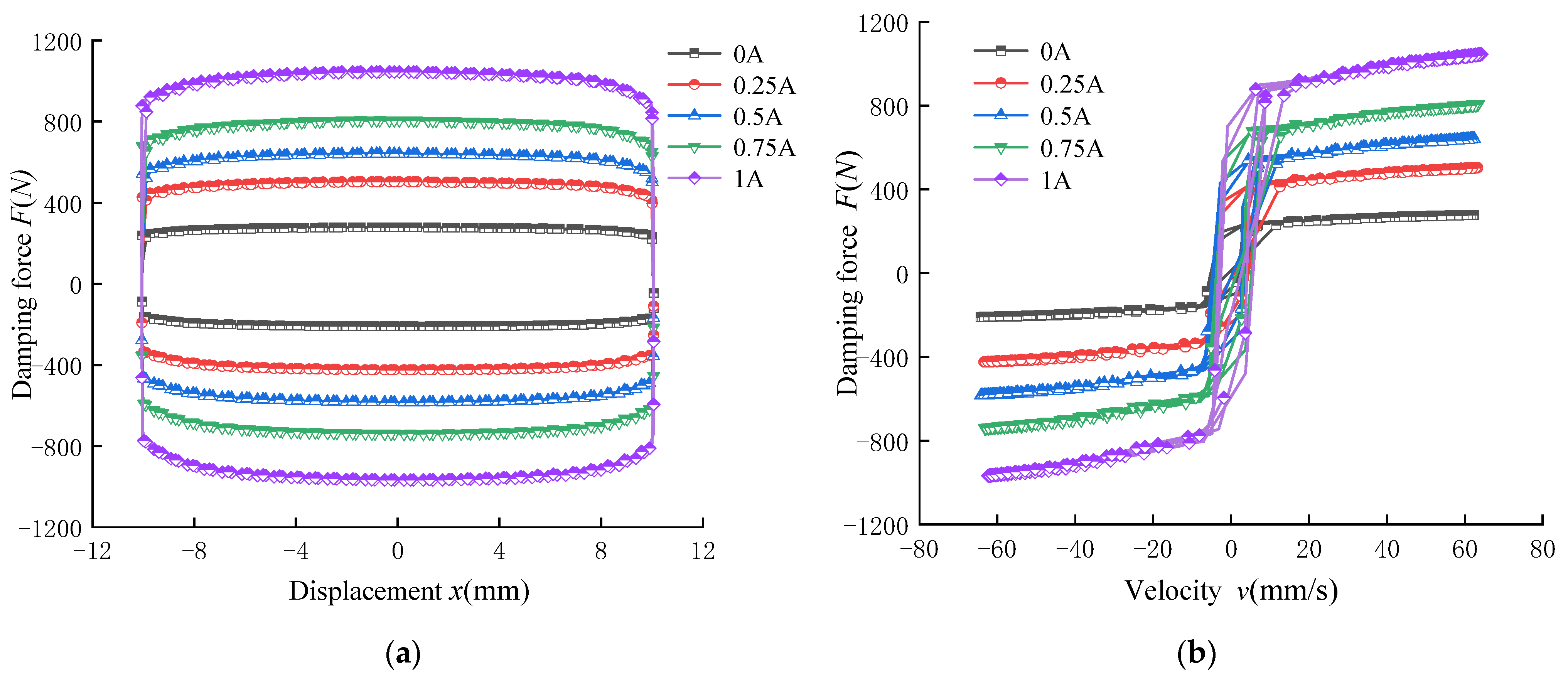
In this experiment, a sinusoidal excitation signal with a frequency of 1 Hz and amplitudes of 5 mm, 7.5 mm, 10 mm was adopted. The currents were 0 A, 0.25 A, 0.5 A, 0.75 A and 1 A, provided by a DC regulated power supply. As shown in Figure 2, the variation of the output damping force with displacement and velocity of the MR damper under different excitation currents is obtained. Figure 2a shows that the output damping force of the MR damper increases with the increase in the excitation current. This is mainly because the magnetic flux density in the damping channel increases with the increase in the excitation current. The output damping force varies little with the displacement, and it is distributed symmetrically with respect to the relative equilibrium position. As shown in Figure 2b, the damping force of the MR damper increases with the increase in the excitation current and vibration speed, but the influence of the speed is much smaller than that with the current. The proposed MR damper has a wide range of damping force adjustments, and thus, it can be used in a vehicle suspension system.

2.2. Improved Hyperbolic Tangent Model of MR Damper

The improved hyperbolic tangent model can comprehensively describe the damping characteristics of the MR damper. Compared with the hyperbolic tangent model, the physical quantities of this model have a clearer physical significance, and there are fewer unknown parameters, which makes it easy for subsequent parameter identification. The improved hyperbolic tangent model is shown in Figure 3, and its mathematical expression is as follows:

$$F=a_1\tanh [a_2(\dot{x}+kx)]+a_3(\dot{x}+kx)+f_0$$

(1)

where a₁ and k are both proportional factors, a₁ is related to the current and k affects the width of the hysteresis loop; a₂ and a₃ are damping coefficients that affect the curve variation trend of the pre-yield zone and post-yield zone, respectively; and f₀ denotes the offset damping force.

2.3. Improved Parameter Identification of Hyperbolic Tangent Model

Figure 4 shows the parameter identification process using the genetic algorithm. Taking the mean square deviation of the difference between the actual damping force and the simulated damping force as the objective function, the smallest mean square deviation is the optimal solution, and the optimal model of the MR damper is obtained through genetic operation selection, crossover and mutation.

The fitness function of the improved hyperbolic tangent model is denoted as follows:

$$fitnessfunc=\frac{1}{m}{\displaystyle {\sum }_{i=1}^m{(F_{simi}-F_{\exp i})}^2}$$

(2)

where F_simi and F_expi are the simulation damping forces and experimental damping forces of the ith point, respectively, and m is the number of experimental points.

The identification parameters were processed by using the real coding method. The scattered crossover method was used to determine the crossover probability by repeated experiments, and the crossover probability was set to 0.8. To improve the local search ability of the genetic algorithm, the Gaussian function was used for mutation with a scale of 0.5 as well as a shrink of 0.7, and the number of iterations was 100.

The improved hyperbolic tangent model has five parameters to be identified, which is expressed as follows:

$$\mathsf{\Theta }=[a_1,a_2,k,a_3,f_0]$$

(3)

The test results of the mechanical characteristics of the MR damper under sinusoidal excitation with an amplitude of 10 mm and frequency of 1 Hz were selected as the identification data. Parameter identification was carried out for the data of 5 groups under different control currents so as to obtain parameter identification results under different current, as shown in

Table 1. Parameter identification results of MR damper model.

Applied Current/(A)	Parameter Values
	a1	a2	k	a3	f0
0	165.94	3890.24	0.3006	849.617	35.68
0.25	366.04	3859.98	0.3001	1548.13	39.69
0.5	483.51	3895.93	0.3004	2045.21	35.06
0.75	615.02	3859.26	0.3000	2573.25	35.07
1.0	805.25	3866.50	0.3001	3301.38	35.09

. By comparing and analyzing the identification results of different current parameters, the variation rules of each parameter were found, and the fitting values of each parameter in the improved hyperbolic tangent model were also obtained.

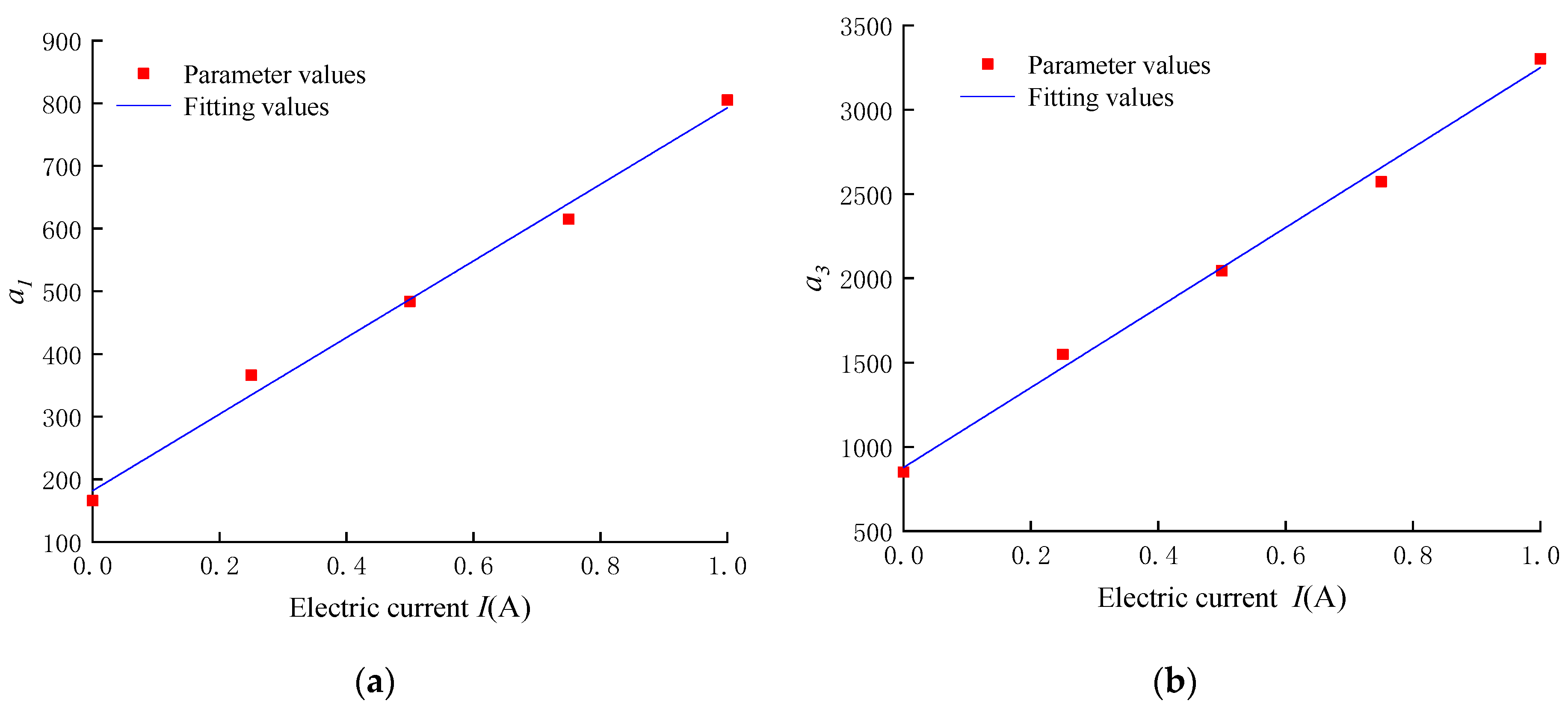
Observing Table 1, parameters a₂, k, and f₀ are not changed significantly under the different current. Therefore, a₂, k, and f₀ can be considered constant values, and their mean values a₂ = 3874.38, k = 0.31, and f₀ = 36.12 are selected. Parameters a₁ and a₃ increase linearly with the increase in current, and the relationship between the parameters and current is obtained through fitting, as shown in Figure 5.

As shown in Figure 5, parameters a₁ and a₃ are linearly correlated with the current, which can be obtained by linear fitting as shown below:

$$\{\begin{array}{l}{a}_1=m_{1}I+n_1=611.04I+181.63\\ a_3=m_{2}I+n_2=2371.46I+877.79\end{array}$$

(4)

The expression of the improved hyperbolic tangent model after parameter identification is obtained as follows:

$$F=(m_{1}I+n_1)\tanh (a_2(\dot{x}+kx))+(m_{2}I+n_2)(\dot{x}+kx)+f_0$$

(5)

According to the improved hyperbolic tangent model expressed in Equation (5) after parameter identification, the mechanical properties of the MR damper was simulated and compared with the test results, as shown in Figure 6. The force–displacement curve of the improved hyperbolic tangent model after parameter identification has a high degree of fit with the test curve. For the force–velocity curve, the nonlinear hysteretic characteristics of the MR dampers in low, and the high-speed regions are well described. Therefore, the hyperbolic tangent model can be applied to the subsequent semi-active control.

2.4. ANFIS Inverse Model of MR Damper

The ANFIS is a multilayer feedforward network that uses neural network learning algorithms and fuzzy reasoning to map an input space to an output space [29]. The ANFIS algorithm has a strong adaptive ability and self-learning ability, and it has a strong approximation ability to the nonlinear system. Therefore, ANFIS is suitable for the modeling of complex systems, such as MR dampers. Figure 7 shows the structure of ANFIS. There are five layers in total, and the function types of the nodes in each layer are the same.

Layer 1 is used to fuzzify the input signal, and its node output is defined as follows:

$$\{\begin{array}{c}{o}_{1,i}={\mu }_{A_i}(x),i=1,2 or\\ o_{1,i}={\mu }_{B_{i-2}}(x),i=3,4\end{array}$$

(6)

where o_1,i is the output of the ith node of layer 1, and x represents the input of the node, respectively. A_i (or B_i−2) represents fuzzy sets (negative big, negative small, positive big, positive small, etc.). The membership function of the fuzzy set is as follows:

$${\mu }_{A_i}(x)=\frac{1}{1+{\left(\frac{x-c_i}{a_i}\right)}^{2b_i}},{\mu }_{B_{i-2}}(x)=\frac{1}{1+{\left(\frac{y-c_i}{a_i}\right)}^{2b_i}}$$

(7)

The above equation is bell-shaped functions (the maximum is 1, the minimum is 0), where $\left\{a_i,b_i,c_i\right\}$ is the premise parameter used to adjust the shape of the function.

Layer 2 is represented by π, whose function is to calculate the applicability of each rule w_i. The specific operation is to take the product of the membership degree of each input signal as the applicability of this rule, as shown in the equation below.

$$o_{2,i}=w_i={\mu }_{A_i}(x)\times {\mu }_{B_i}(y),i=1,2$$

(8)

Layer 3 is represented by circle N as shown in the Figure 7. Layer 3 is used to normalize the applicability of each rule, as shown in Equation (9).

$$o_{3,i}={\overline{w}}_i=\frac{w_i}{w_1+w_2},i=1,2$$

(9)

The function of Layer 4 is to calculate the output of each rule. The node function is expressed as follows:

$$o_{4,i}={\overline{w}}_i{f}_i={\overline{w}}_i(p_{i}x+q_{i}y+r_i), i=1,2$$

(10)

where parameters $\left\{p_i,q_i,r_i\right\}$ represent an adjustable parameter set.

Layer 5 sums up all the inputs of the node and outputs the results to calculate the total output of the system.

$$o_{5,i}={\displaystyle \sum _{i=1}^2{\overline{w}}_i{f}_i=\frac{{\displaystyle \sum _{i=1}^2{w}_i{f}_i}}{{\displaystyle \sum _{i=1}^2{w}_i}}}$$

(11)

ANFIS can obtain the required fuzzy rules and membership function after repeated training based on a large amount of data. Usually, the BP algorithm or hybrid algorithm is used to train the data.

The adaptive neuro fuzzy inference system (ANFIS) was used to establish the inverse model of the MR damper in this paper [30]. The training schematic diagram of the ANFIS inverse model of the MR damper is shown in Figure 8. In order to establish the inverse model of ANFIS, the velocity, displacement and expected damping force at the current moment as well as the velocity and desired damping force provided by the forward model at the previous moment were selected as the input, while the control current at the current moment was taken as the output.

Two sets of data were needed to model a MR damper, using an adaptive neuro-fuzzy reasoning system. One set was used to train the inverse model of ANFIS, and the other set was used to test the accuracy of the model. A sinusoidal function with an amplitude of 20 mm was used for the displacement signal, and a sinusoidal function with an amplitude of 0~2 A was used for the control current signals. There were 1500 data points of which 1000 points were used for training and 500 points were used for validation.

Figure 9 and Figure 10 show the comparison between the experimental and predicted values as well as the error of the ANFIS inverse dynamics model of the MR damper, respectively. The results illustrate that the predictive control current of the ANFIS inverse model can track the target control current well, and verify the effectiveness of the model.

3. Modeling of Quarter Vehicle MR Semi-Active Air Suspension System

3.1. Elastic Model of Air Spring

The principle of the air suspension vehicle is that the air spring uses the air compressibility to play a supporting role. The vertical supporting force F_v produced by the air spring is the following:

$$F_v=PA$$

(12)

where P is the air pressure in the airbag, and A is the effective bearing area.

The air spring moves vertically in the process of working, and the air spring bag is stretched or compressed, due to the change in volume. This process exchanges heat with the outside world. Assuming that the time required for the movement of the air spring is short enough, it can be regarded as an adiabatic process [31]. The state equation of the gas at this time can be regarded as follows:

$$(P+P_a)V^m=(P_a+P_0)V_0^m$$

(13)

where V₀ is the volume of the air spring in the initial state, V is the working volume of the air spring, P₀ is the gas pressure in the initial state of the air spring, and P_a is the standard atmospheric pressure.

According to Equation (13), the pressure in the air bag can be obtained as follows:

$$P=(P_0+P_a){\left(V_0/V\right)}^m-P_a$$

(14)

Substituting Equations (13) and (14) to Equation (12), it can be derived as follows:

$$F=[{\left(V_0/V\right)}^m(P_0+P_a)-P_a]A$$

(15)

When the air spring works, its volume and bearing area are related to the displacement, and thus, taking the derivative of Equation (15) with respect to the displacement, the stiffness k_a of the air spring is yielded, and it can be regarded as follows:

$$k_a=\frac{dF}{dx}=P\frac{dA}{dx}-A\frac{m}{V}(P+P_a)\frac{dV}{dx}$$

(16)

When the air spring is in an equilibrium state, there are the following relations:

$$P=P_0,A=A_0,V=V_0$$

Therefore, the air spring stiffness k₀ under an equilibrium state is obtained as follows:

$$k_0=p_0\frac{dA}{dx}-A_0\frac{m}{V}(p+p_a)\frac{dV}{dx}$$

(17)

The natural frequency of the air spring is the following:

$$f_0=\frac{1}{2\pi }\sqrt{\frac{k_0}{m}}$$

(18)

3.2. Modeling of Quarter Vehicle MR Semi-Active Air Suspension System

Passive suspension is mainly composed of a passive damper and spring with immutable stiffness, and its structure is relatively simple, as shown in Figure 11. The damping force and stiffness of passive suspension cannot be adjusted in real time with different road surface and vehicle parameters. Under a certain suspension relative speed, only a fixed suspension output damping force can be provided. Therefore, the vibration damping capacity of passive suspension decreases significantly, and its road adaptability is poor under a certain range of road surface conditions, especially on a bad road surface.

Figure 12 shows the model of a quarter vehicle MR semi-active air suspension system, which is composed of a car body (sprung mass), wheel (unsprung mass), tire stiffness, damping and suspension stiffness.

According to Newton’s second law, the motion equation of the system is as follows:

$$\{\begin{array}{l}{m}_b{\ddot{x}}_b+k_a(x_b-x_w)+c_0({\dot{x}}_b-{\dot{x}}_w)=f_d\hfill \\ m_w{\ddot{x}}_w+k_a(x_w-x_b)+c_0({\dot{x}}_w-{\dot{x}}_b)+k_t(x_w-x_t)=-f_d\hfill \end{array}$$

(19)

where m_b and m_w are the mass of the sprung body and the unsprung wheel, respectively, k_a is the stiffness of the air spring, k_t is the stiffness of the tire, x_b is the displacement of the mass of the body, x_w is the displacement of the wheel, x_t is the displacement of the road surface excitation, and f_d depicts the output damping force of the MR damper.

The system state variable can be denoted as follows:

$$x=(x_b,x_w,{\dot{x}}_b,{\dot{x}}_w)$$

(20)

The output variable can be depicted as follows:

$$y=({\ddot{x}}_b,x_b-x_w,k_t(x_w-x_t))$$

(21)

where ${\ddot{x}}_b$ is the acceleration of the car body, x_b − x_w is the dynamic deflection of the suspension, and k_t(x_w − x_t) is the dynamic load of the tire.

The state space expression of the suspension system is as follows:

$$\{\begin{array}{c}\dot{x}=Ax+Bu\\ y=Cx+Du\end{array}$$

(22)

where

$$A=\left[\begin{array}{cccc}0& 0& 1& 0\\ 0& 0& 0& 1\\ -\frac{k_a}{m_b}& \frac{k_a}{m_b}& -\frac{c_0}{m_b}& \frac{c_0}{m_b}\\ -\frac{k_a}{m_w}& -\frac{k_a+k_t}{m_w}& \frac{c_0}{m_w}& -\frac{c_0}{m_w}\end{array}\right], B=\left[\begin{array}{cc}0& 0\\ 0& 0\\ 0& \frac{1}{m_b}\\ \frac{k_t}{m_w}& -\frac{1}{m_w}\end{array}\right]$$

$$C=\left[\begin{array}{cccc}-\frac{k_a}{m_b}& \frac{k_a}{m_b}& -\frac{c_0}{m_b}& \frac{c_0}{m_b}\\ 1& -1& 0& 0\\ 0& k_t& 1& 0\end{array}\right], D=\left[\begin{array}{cc}0& \frac{1}{m_b}\\ 0& 0\\ -k_t& 0\end{array}\right]$$

4. Design of Sliding Mode Controller for MR Semi-Active Air Suspension

4.1. Reference Model of Sliding Mode Controller

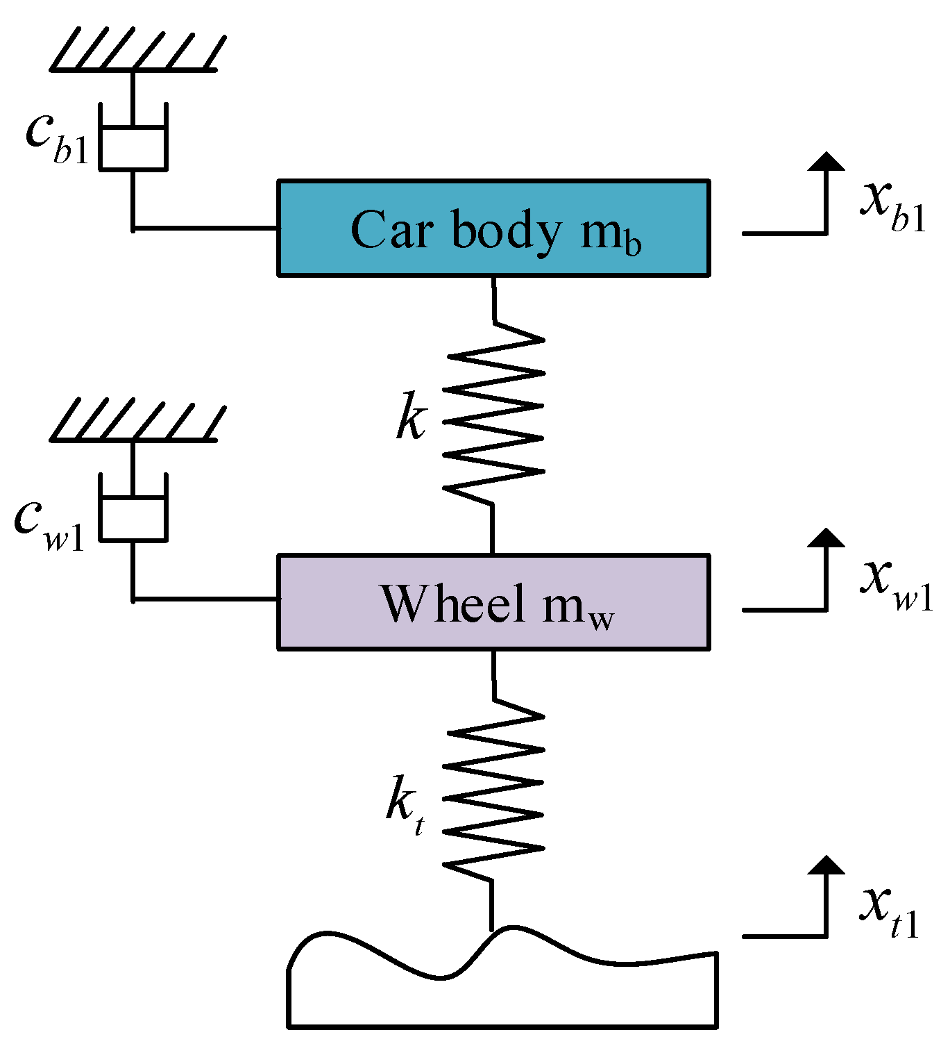
Figure 13 is the reference model of sliding model controller based on the knowledge of optimal control theory proposed by Karnopp [32], which has excellent robustness and excellent control performance. According to Newton’s second law, the dynamic differential equation is as follows:

$$\{\begin{array}{l}{m}_b{\ddot{x}}_{b1}+k(x_{b1}-x_{w1})+c_{b1}{\dot{x}}_{b1}=0\hfill \\ m_w{\ddot{x}}_{w1}+k(x_{w1}-x_{b1})+k_t(x_w-x_t)+c_{w1}{\dot{x}}_{w1}=0\hfill \end{array}$$

(23)

where m_b and m_w represent sprung body mass and unsprung wheel mass, respectively; k and k_t denote the spring stiffness and tire stiffness, respectively; x_b1, x_w1, and x_t1 are the body displacement, wheel displacement and displacement of the road surface excitation, respectively; and c_b1 and c_w1 are the damping coefficients.

The state variables are selected as follows:

$$X_1={[x_{b1},x_{w1},{\dot{x}}_{b1},{\dot{x}}_{w1}]}^T$$

(24)

Substituting Equation (24) into Equation (23), it can be obtained the following:

$${\dot{X}}_1=A_1{X}_1+E_1\omega$$

(25)

where

$$A_1=\left[\begin{array}{cccc}0& 0& 1& 0\\ 0& 0& 0& 1\\ -\frac{k_t+k}{m_w}& \frac{k}{m_w}& -\frac{c_{b1}}{m_w}& 0\\ \frac{k}{m_b}& -\frac{k}{m_b}& 0& -\frac{c_{b1}}{m_b}\end{array}\right], E_1=\left[\begin{array}{c}0\\ 0\\ \frac{k_t}{m_w}\\ 0\end{array}\right], \omega =x_{t1}$$

4.2. Design of Sliding Mode Controller

The design principle of the sliding mode controller (SMC) is to make the actual controlled system track the motion of the reference system and produce the sliding mode in the error dynamics system between the actual controlled system and the reference system. The error vector e of the air suspension system is defined as the velocity error, displacement error and integral of displacement error, and its matrix form can be expressed as follows:

$$e={[\begin{array}{ccc}{\dot{x}}_b-{\dot{x}}_{b1}& x_b-x_{b1}& {\displaystyle \int (x_b-x_{b1})}\end{array}]}^T$$

(26)

$$\dot{e}={[\begin{array}{ccc}{\ddot{x}}_b-{\ddot{x}}_{b1}& {\dot{x}}_b-{\dot{x}}_{b1}& x_b-x_{b1}\end{array}]}^T$$

(27)

Therefore, the error dynamics equation is defined as follows:

$$\dot{e}=A(t)e+B(t)X+H(t)X_r+G(t)u$$

(28)

In the design of switching the surface of the sliding mode variable structure, the pole assignment method is generally used to set the function of the switching surface. The output value of the controller is the controllable damping force, and thus its switching surface can be expressed as follows:

$$s=cx[c_1,c_2,\cdots ,c_n]·{[x_1,x_2,\cdots ,x_n]}^T$$

(29)

Parameter n is 3, so the sliding mode switching surface function is as follows:

$$s=ce$$

(30)

The state Equation (29) is simplified as follows:

$$\left[\begin{array}{c}{s}_1\\ s_2\end{array}\right]=\left[\begin{array}{l}0 1\\ -c_1 -c_2 \end{array}\right]\left[\begin{array}{l}{e}_1\\ e_2\end{array}\right]$$

(31)

All control points of sliding mode motion must have good dynamic quality and be asymptotically stable when entering the sliding mode switching surface. Equation (31) is the motion differential equation of the sliding mode, and its characteristic equation is as follows:

$$D(\lambda )={\lambda }^2+c_2\lambda +c_1$$

(32)

The values of c₁ and c₂ can be obtained by making the characteristic root equal to the given pole.

The transfer function in standard form for a second-order system is as follows:

$$\mathrm{\Phi }(s)=\frac{Y(s)}{U(s)}=\frac{{\omega }_n{}^2}{s^2+2\xi {\omega }_{n}s+{\omega }_n{}^2}$$

(33)

The two closed-loop poles of the system are $s_{1,2}=-\xi {\omega }_n\pm j{\omega }_n\sqrt{1-{\xi }^2}$. Only when the pole is on the left half of the complex plane does the control system have partial oscillations. The desired number of poles n is set as 3. Among them, the dynamic performance of the control system is determined by the dominant pole, and the far pole has little influence on it. It can be obtained that the characteristic root of the system is −3.9 ± 5.2j, under the condition of $\sigma \le 15\%$, $t_p\le 0.7$, ${\omega }_n=6.5$, and $\xi =0.6$. Then, c = [42.25, 7.8, 1] can be obtained.

Therefore, the switching surface function of MR semi-active air suspension is as follows:

$$s=[\begin{array}{ccc}({\dot{x}}_b-{\dot{x}}_{b1})& c_1(x_b-x_{b1})& c_2({\displaystyle \int (x_b-x_{b1})}\end{array}){]}^T$$

(34)

According to Equation (30), it can be obtained as follows:

$$\dot{s}=c\dot{e}=cA(t)e+cB(t)X+cH(t)X_r+cG(t)u$$

(35)

From the above, it can be developed as follows:

$$U={(cG)}^{-1}[\dot{s}-(cA(t)e+cB(t)X+cH(t)X_r]$$

(36)

To minimize the error between the actual controlled model and the reference model, let $\dot{s}$ be 0, and Equation (36) can be deduced as follows:

$$U={(cG)}^{-1}[(cA(t)e+cB(t)X+cH(t)X_r]$$

(37)

The equivalent output damping force of the sliding mode controller can be obtained as follows:

$$U_{eq}=(c_0-c_1{m}_b)({\dot{x}}_b-{\dot{x}}_{b1})+(k_a-c_2{m}_w)(x_b-x_{b1})-k_a(x_w-x_{w1})-c_0({\dot{x}}_w-{\dot{x}}_{w1})$$

(38)

To improve sliding mode motion, the reaching law is defined as follows:

$$\dot{s}=-\epsilon \cdot \mathrm{sgn}(s), (\epsilon >0)$$

(39)

where sgn(s) is a sign function, and ε is the rate of control point approaching the switching surface, which affects the system stability. The smaller ε is, the smaller the approaching rate is, while the larger ε is, the greater the approaching rate is, and the more severe the system chattering is. In the sliding mode control, ε is 0.1 according to the experience and debugging results.

The system stability was verified according to the Lyapunov stability criterion. If V(x) is positive definite and $\dot{V}(x)$ is negative definite, the system is stable. Select the Lyapunov function as follows:

$$V(x)=\frac{1}{2}{s}^{T}s$$

(40)

Then it can be derived as follows:

$$\dot{V}(x)=s^T\dot{s}=s^T(-\epsilon \mathrm{sgn}(s))\le 0$$

(41)

According to the Lyapunov stability criterion, it can be inferred that the system is stable. Therefore, the final sliding mode control law of the system is as follows:

$$U=U_{eq}+U_{sw}=U_{eq}+{[cG]}^{-1}\dot{s}=U_{eq}+\epsilon m_s\mathrm{sgn}(s)$$

(42)

where m_s is the coefficient related to s and $\dot{s}$.

Finally, the variable damping force by the sliding mode controller is as follows:

$$U_d=\{\begin{array}{cc}{U}_{eq}+U_{sw}& [U_{eq}+U_{sw}]({\dot{x}}_b-{\dot{x}}_{b1})\ge 0\\ 0& [U_{eq}+U_{sw}]({\dot{x}}_b-{\dot{x}}_{b1})\le 0\end{array}$$

(43)

4.3. Design of Fuzzy Sliding Mode Controller

The structure diagram of FSMC is shown in Figure 14. In order to make the controlled system track the motion of the reference system, the sliding mode switching surface function s is designed according to the error between the controlled system and the reference system. The equivalent output damping force U_eq of the sliding mode controller can be obtained. At the same time, ε and the switching control force U_sw are obtained by the fuzzy controller. Finally, the force required for the damper (predictive damping force) can be obtained. According to the inverse model of the damper, the control current is obtained, and the actual control force is generated by controlling the MR damper.

In the fuzzy system, $s$ and $\dot{s}$ are defined as inputs of the fuzzy controller, and the output value of the fuzzy controller is defined as ε of the sliding mode controller. As shown in Figure 15, the fuzzy domain of the fuzzy input and output is set as {−3, −2, −1, 0, 1, 2, 3}. Language variables describing input and output variables are divided into seven levels: NB (negative big), NM (negative medium), NS (negative small), ZE (zero), PS (positive small), PM (positive medium), and PB (positive big). The triangular membership function is selected as the membership function of fuzzy input S, SC and output E, respectively.

If the controller satisfies the conditions of $s\dot{s}<0$, the fuzzy control rules shown in

Table 2. Fuzzy control rules.

		SC	NB	NM	NS	ZE	PS	PM	PB
	C
S
NB			NB	NB	NM	NM	NS	NS	ZE
NM			NB	NB	NM	NS	NS	NS	ZE
NS			NM	NM	NS	ZE	ZE	ZE	ZE
ZE			NM	NM	NS	ZE	ZE	PS	PS
PS			NS	NS	ZE	ZE	PS	PS	PM

are established. The control target can be expressed as follows:

$$U=-{(cG)}^{-1}c[A(t)e+G(t)X+H(t)X_r]+{\epsilon }_{fuzzy}{m}_s\mathrm{sgn}(s)$$

(44)

where ${\epsilon }_{fuzzy}$ is the output of the fuzzy sliding mode controller.

5. Simulation Analysis of Fuzzy Sliding Mode Control

5.1. Random Road Excitation Response

In order to verify the effectiveness of the FSMC method, the random road excitation was selected as the road input for simulation analysis. The white noise signal after the forming filter was usually used as the time domain signal of the random road surface. The real road surface of vehicle driving can be regarded as follows:

$$\dot{q}(t)=-2\mathsf{\pi }{f}_{1}q(t)+2\mathsf{\pi }{n}_0\sqrt{G_q(n_0)v}w(t)$$

(45)

where f₁ is the lower cutoff frequency of the road filter, q(t) donates the road surface excitation, G_q(n₀) is the road roughness coefficient, w(t) is the white noise with a covariance of 1, and v is the vehicle speed.

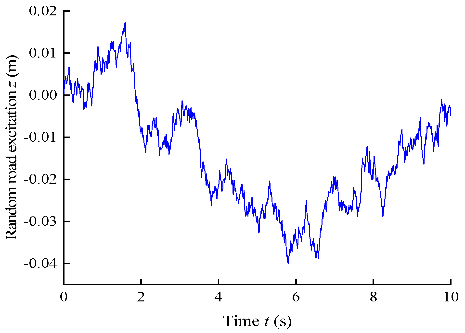
In the simulation analysis, MATLAB software was used for numerical simulation of the system, in which the sampling period is 0.001 s. Figure 16 shows the random input waveform of the road surface, using the filtering white noise generation method, where f₁ is 0.01 Hz, the C-level road roughness coefficient G_q(n₀) is 256 × 10⁻⁶ m³, and the vehicle velocity v is 20 m/s.

Table 3. Model parameters of two-degree-of-freedom quarter vehicle passive air suspension system.

Parameters	Symbol	Unit	Values
Sprung mass	mb	kg	400
Unsprung mass	mw	kg	40
Tire damping	Kt	N/m	170,000
Damping coefficient	Cb1	N/(m/s)	3550
Damping coefficient	Cw1	N/(m/s)	3550
Suspension stiffness	K	N/m	17,000
Initial volume of air spring	V0	m3	0.0078
Initial area of air spring	A0	m2	0.0381
Initial pressure of air spring	P0	MPa	0.382

shows the parameters of semi-active air suspension system required for simulation.

Figure 17 shows the time domain of the 2-DOF quarter vehicle semi-active air suspension controlled by the FSMC method. The random road excitations of passive suspension, SMC control and FSMC control suspension are the same, shown in Figure 16. It can be seen that the semi-active air suspension controlled by FSMC switching has significantly improved the damping performance, compared with the passive suspension and the semi active air suspension controlled by SMC.

Table 4. RMS values of suspension system indexes under random road excitation.

Control Strategies	Body Acceleration	Suspension Stroke	Tire Dynamic Load
Passive suspension	0.857	7.73	307.5
SMC control	0.721	6.42	284.6
FSMC control	0.634	5.46	282.1

shows the root mean square (RMS) values of the air suspension performance indexes under a random road surface. Compared with passive suspension, the body acceleration under SMC control and FSMC control decreases by 15.9% and 26%, respectively, the suspension dynamic travel decreases by 16.9% and 29.4%, respectively, and the wheel dynamic load decreases by 7.4% and 8.4%, respectively.

Figure 18 shows the power spectral density (PSD) under the input of random road surface. In the high frequency range, the power spectral density of FSMC control and sliding mode control is similar to that of the passive system in terms of body acceleration, suspension dynamic travel and tire dynamic load, due to frequency conversion interference. However, in the low frequency domain where the body is sensitive to the resonance of the car body, the 2-DOF quarter car semi-active air suspension controlled by FSMC is obviously superior to the controlled suspension and the sliding mode control suspension, the occupant’s comfort is enhanced, and the resonance of the car body is effectively prevented.

5.2. Impacted Pavement Excitation Response

Vehicle driving is not only the existence of random continuous vibration; sometimes, there will be low-lying, protrusion sections, which bring strong impact to the vehicle. Therefore, in order to fully reflect the vibration reduction ability of the vehicle suspension system, the impact road surface model was established to replace the impact vibration of the vehicle on the road surface. Figure 19 shows the simulation curve of impact road surface input, and its mathematical model is as follows:

$$x_0(t)=\{\begin{array}{cc}\frac{H}{2}\left[1-\cos \left(\frac{2\pi u}{W_0}t\right)\right]& \frac{W_0}{u}\le t\le \frac{2W_0}{u}\\ 0& other\end{array}$$

(46)

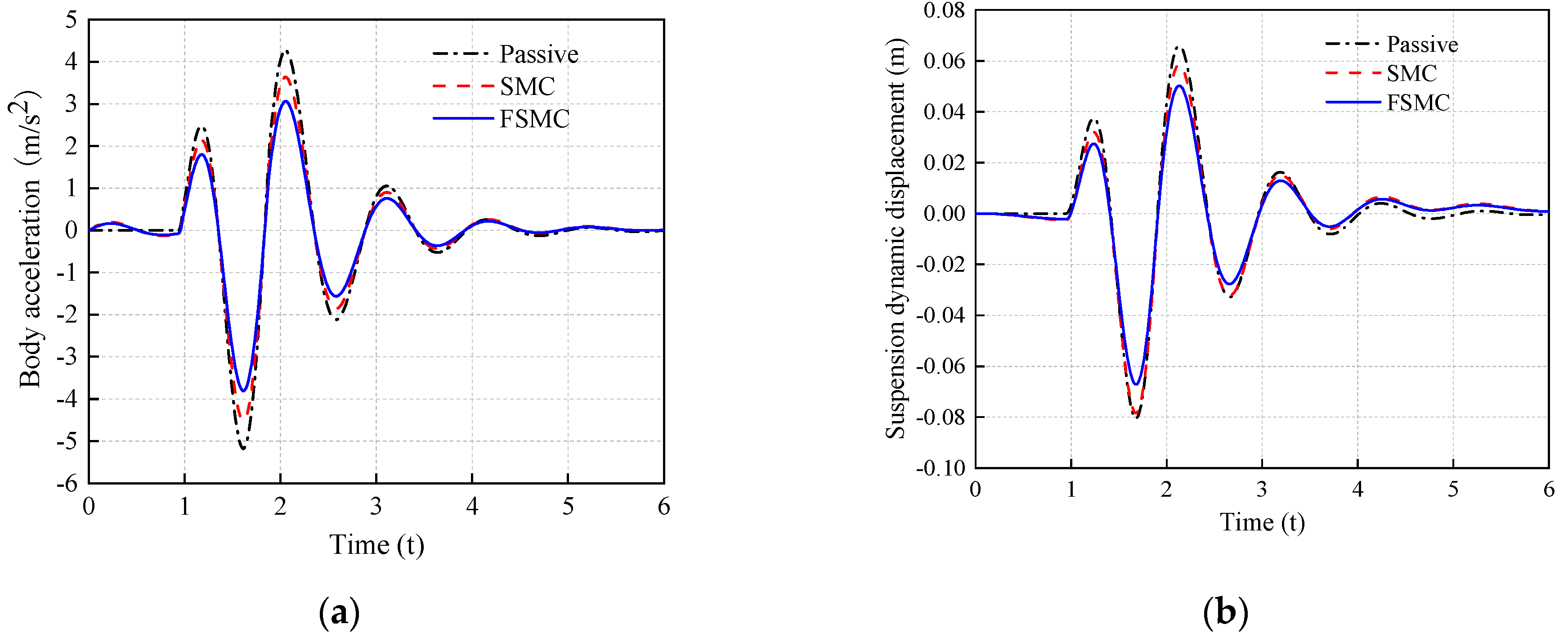
where x₀(t) represents the input displacement of the impact road, H is the height of the impact road with a value of 0.07 m, W₀ represents the width of the impact road with a value of 0.08 m, u donates the vehicle speed, and the value is 3.08 km/h.

The simulation curve of the 2-DOF quarter vehicle semi-active air suspension controlled by FSMC impacting the road surface is shown in Figure 20. It reflects that the peak value of the FSMC-controlled semi-active air suspension is significantly reduced, compared with that of the passive and SMC-controlled semi-active air suspension under the same impact road excitation.

Compared with passive suspension, the peak reduction percentages of body acceleration, suspension dynamic travel and wheel dynamic load of semi-active suspension under SMC control and FSMC control are shown in Figure 21, in which the body acceleration under SMC control and FSMC control are 13.9% and 27.5%, respectively, lower than that of passive suspension. The suspension dynamic travel is reduced by 12.8% and 26.5%, respectively, while the wheel dynamic load is reduced by 5% and 9.6%, respectively.

6. Conclusions

Based on the experimental data, the parameters of the improved hyperbolic tangent model were identified by the genetic algorithm, and the magnetic parameter identification results were consistent with the experimental data. The identified parameters of the improved hyperbolic tangent model could be used in semi-active control. The predictive control current of ANFIS inverse model can track the target control current well, which verifies the effectiveness of the model.

The semi-active air suspension system model of quarter vehicle equipped with MR damper was established, and the feasibility of the FSMC strategy was verified by taking the random road excitation and impact road excitation as input. Compared with the passive suspension, the vehicle acceleration under SMC control and FSMC control is reduced by 15.9% and 26%, respectively; the suspension dynamic travel is reduced by 16.9% and 29.4%, respectively; and the wheel dynamic load is reduced by 7.4% and 8.4%, respectively, under random road excitation. With the impact of road excitation, the peak acceleration of the vehicle based on SMC control and FSMC control decreases by 13.9% and 27.5%, respectively; the peak dynamic travel of suspension decreases by 12.8% and 26.5%, respectively; and the peak dynamic load of tire decreases by 5% and 9.6%, respectively, compared with the passive suspension. It can be concluded that the control strategy proposed in this article has a better damping effect and can improve the driving comfort and stability of the vehicle.

References

- Nguyen, S.D.; Bao, D.L.; Ngo, V.H. Fractional-order sliding-mode controller for semi-active vehicle MRD suspensions. Nonlinear Dyn. 2020, 101, 795–821. [Google Scholar] [CrossRef]
- He, F.; Zhao, J.; Wang, H.Y. Study on control strategies of semi-active air suspension for heavy vehicles based on road-friendliness. Adv. Mater. Res. 2012, 452, 328–333. [Google Scholar] [CrossRef]
- Zhang, Z.; Wang, J.; Wu, W.; Huang, C. Semi-active control of air suspension with auxiliary chamber subject to parameter uncertainties and time-delay. Int. J. Robust. Nonlinear Control 2020, 30, 7130–7149. [Google Scholar] [CrossRef]
- Gokul, P.S.; Malar, M.K. A contemporary adaptive air suspension using LQR control for passenger vehicles. ISA Trans. 2019, 93, 244–254. [Google Scholar]
- Fan, S.Y.; Chuang, C.W.; Feng, C.C. Apply Novel Grey Model Integral Variable Structure Control to Air-Ball-Suspension System. Asian. J. Control 2016, 18, 1359–1364. [Google Scholar] [CrossRef]
- Elsaady, W.; Oyadiji, S.O.; Nasser, A. Magnetic circuit analysis and fluid flow modeling of an MR damper with enhanced magnetic characteristics. IEEE Trans. Magn. 2020, 56, 1–20. [Google Scholar] [CrossRef]
- Hu, G.; Yi, F.; Liu, H.; Zeng, L. Performance analysis of a novel magnetorheological damper with displacement self-sensing and energy harvesting capability. J. Vib. Eng. Technol. 2021, 9, 85–103. [Google Scholar] [CrossRef]
- Hu, G.; Yi, F.; Tong, W.; Yu, L. Development and evaluation of a MR damper with enhanced effective gap lengths. IEEE Access 2020, 8, 156347–156361. [Google Scholar] [CrossRef]
- Sun, S.S.; Ning, D.H.; Yang, J.; Du, H.; Zhang, S.W.; Li, W.H. A seat suspension with a rotary magnetorheological damper for heavy duty vehicles. Smart Mater. Struct. 2016, 25, 105032. [Google Scholar] [CrossRef]
- Wang, D.H.; Liao, W.H. Magnetorheological fluid dampers: A review of parametric modelling. Smart Mater. Struct. 2011, 20, 023001. [Google Scholar] [CrossRef]
- Mughal, U.N. State of the art review of semi active control for magnetorheological dampers. In Proceedings of the ICNPAA 2016 World Congress, La Rochelle, France, 4–8 July 2016; AIP Publishing LLC: New York, NY, USA, 2016; Volume 1798, p. 020101. [Google Scholar]
- Khalid, M.; Yusof, R.; Joshani, M.; Selamat, H.; Joshani, M. Nonlinear identification of a magneto-rheological damper based on dynamic neural networks. Comput.-Aided Civ. Inf. 2014, 29, 221–233. [Google Scholar] [CrossRef]
- Kwok, N.M.; Ha, Q.P.; Nguyen, T.H.; Li, J.; Samali, B. A novel hysteretic model for MR fluid dampers and parameter identification using particle swarm optimization. Sens. Actuators A Phys. 2006, 132, 441–451. [Google Scholar] [CrossRef]
- Guo, S.; Yang, S.; Pan, C. Dynamic modeling of MR damper behaviors. J. Intell. Mat. Syst. Struct. 2006, 17, 3–14. [Google Scholar] [CrossRef]
- Choi, S.B.; Choi, J.H.; Lee, Y.S.; Han, M.S. Vibration control of an er seat suspension for a commercial vehicle. J. Dyn. Syst. Meas. Control 2003, 125, 60–68. [Google Scholar] [CrossRef]
- Pang, H.; Shang, Y.; Yang, J. An adaptive sliding mode–based fault-tolerant control design for half-vehicle active suspensions using T–S fuzzy approach. J. Vib. Control 2020, 26, 1411–1424. [Google Scholar] [CrossRef]
- Wang, G.; Chadli, M.; Basin, M.V. Practical terminal sliding mode control of nonlinear uncertain active suspension systems with adaptive disturbance observer. IEEE/ASME Trans. Mechatron. 2020, 26, 789–797. [Google Scholar] [CrossRef]
- Fei, J.; Xin, M. Robust adaptive sliding mode controller for semi-active vehicle suspension system. Int. J. Innov. Comput. Inf. Control 2012, 8, 691–700. [Google Scholar]
- Du, M.; Zhao, D.; Yang, B.; Wang, L. Terminal sliding mode control for full vehicle active suspension systems. J. Mech. Sci. Technol. 2018, 32, 2851–2866. [Google Scholar] [CrossRef]
- Nguyen, S.D.; Lam, B.D.; Choi, S.B. Smart dampers-based vibration control-Part 2: Fractional-order sliding control for vehicle suspension system. Mech. Syst. Signal. Pract. 2021, 148, 107145. [Google Scholar] [CrossRef]
- Zheng, L.; Li, Y.N.; Baz, A. Fuzzy-sliding mode control of a full car semi-active suspension systems with MR dampers. Smart Struct. Syst. 2009, 5, 261–277. [Google Scholar] [CrossRef]
- Wang, R.; Liu, W.; Ding, R.; Meng, X.; Sun, Z.; Yang, L.; Sun, D. Switching control of semi-active suspension based on road profile estimation. Veh. Syst. Dyn. 2021, 1–21. [Google Scholar] [CrossRef]
- Pang, H.; Liu, F.; Xu, Z. Variable universe fuzzy control for vehicle semi-active suspension system with MR damper combining fuzzy neural network and particle swarm optimization. Neurocomputing 2018, 306, 130–140. [Google Scholar] [CrossRef]
- Hu, G.; Liu, Q.; Ding, R.; Li, G. Vibration control of semi-active suspension system with magnetorheological damper based on hyperbolic tangent model. Adv. Mech. Eng. 2017, 9, 1687814017694581. [Google Scholar] [CrossRef]
- Huang, Y.; Na, J.; Wu, X.; Gao, G.; Guo, Y. Robust adaptive control for vehicle active suspension systems with uncertain dynamics. Trans. Inst. Meas. Control 2018, 40, 1237–1249. [Google Scholar] [CrossRef]
- Ming, L.; Yibin, L.; Xuewen, R.; Shuaishuai, Z.; Yanfang, Y. Semi-active suspension control based on deep reinforcement learning. IEEE Access 2020, 8, 9978–9986. [Google Scholar] [CrossRef]
- Ye, H.; Zheng, L. Comparative study of semi-active suspension based on LQR control and H2/H∞ multi-objective control. In Proceedings of the 2019 Chinese Automation Congress (CAC), Hangzhou, China, 22–24 November 2019; pp. 3901–3906. [Google Scholar]
- Rath, J.J.; Veluvolu, K.C.; Defoort, M. Adaptive super-twisting observer for estimation of random road excitation profile in automotive suspension systems. Sci. World J. 2014, 2014, 203416. [Google Scholar] [CrossRef]
- Chang, F.J.; Chang, Y.T. Adaptive neuro-fuzzy inference system for prediction of water level in reservoir. Adv. Water Resour. 2006, 29, 1–10. [Google Scholar] [CrossRef]
- Kim, H.; Lee, H.; Kim, H. Asynchronous and synchronous load leveling compensation algorithm in airspring suspension. In Proceedings of the 2007 International Conference on Control, Automation and Systems, Seoul, Korea, 17–20 October 2007; pp. 367–372. [Google Scholar]
- Liu, H.; Lee, J.C. Model development and experimental research on an air spring with auxiliary reservoir. Int. J. Automot. Technol. 2011, 12, 839–847. [Google Scholar] [CrossRef]
- Karnopp, D.; Crosby, M.J.; Harwood, R.A. Vibration control using semi-active force generators. J. Eng. Ind. 1974, 96, 619–626. [Google Scholar] [CrossRef]
Figure 1.
Vibration test system of MR damper.
Figure 2.
Mechanical characteristics of MR damper. (a) Force displacement, and (b) force velocity.
Figure 3.
Improved hyperbolic tangent model.
Figure 4.
Parameter identification process of MR damper.
Figure 5.
The relation between a1, a3 and current. (a) Parameter a1, (b) parameter a3.
Figure 6.
Comparison of simulation results and experimental tests. (a) Force displacement, and (b) force velocity.
Figure 7.
Structure diagram of ANFIS with two inputs.
Figure 8.
Schematic diagram of the ANFIS inverse dynamics model.
Figure 9.
Verification of training data for ANFIS inverse dynamics model.
Figure 10.
Error of ANFIS inverse dynamics model.
Figure 11.
Model of quarter car passive suspension.
Figure 12.
Model of quarter vehicle air suspension.
Figure 13.
Reference model.
Figure 14.
FSMC structure diagram of MR semi-active air suspension.
Figure 15.
Membership function of input and output variables.
Figure 16.
Random input waveform of road surface.
Figure 17.
Time domain simulation curve of air suspension system under random road excitation. (a) Body acceleration, (b) suspension dynamic deflection, (c) tire dynamic load.
Figure 18.
Simulation curve of power spectral density of air suspension system under random road excitation. (a) Body acceleration, (b) suspension dynamic deflection, (c) tire dynamic load.
Figure 19.
Impacted pavement input simulation curve.
Figure 20.
Simulation curve of air suspension system under impact road excitation. (a) Body acceleration, (b) suspension dynamic displacement, (c) tire dynamic load.
Figure 21.
Percentage reduction of peak response under impacted pavement surface.