An Explainable Approach Based on Emotion and Sentiment Features for Detecting People with Mental Disorders on Social Networks

Abstract

Mental disorders are a global problem that widely affects different segments of the population. Diagnosis and treatment are difficult to obtain, as there are not enough specialists on the matter, and mental health is not yet a common topic among the population. The computer science field has proposed some solutions to detect the risk of depression, based on language use and data obtained through social media. These solutions are mainly focused on objective features, such as n-grams and lexicons, which are complicated to be understood by experts in the application area. Hence, in this paper, we propose a contrast pattern-based classifier to detect depression by using a new data representation based only on emotion and sentiment analysis extracted from posts on social media. Our proposed feature representation contains 28 different features, which are more understandable by specialists than other proposed representations. Our feature representation jointly with a contrast pattern-based classifier has obtained better classification results than five other combinations of features and classifiers reported in the literature. Our proposal statistically outperformed the Random Forest, Naive Bayes, and AdaBoost classifiers using the parser-tree, VAD (Valence, Arousal, and Dominance) and Topics, and Bag of Words (BOW) representations. It obtained similar statistical results to the logistic regression models using the Ensemble of BOWs and Handcrafted features representations. In all cases, our proposal was able to provide an explanation close to the language of experts, due to the mined contrast patterns.

1. Introduction

According to the World Health Organization (WHO), an estimated 264 million people around the world suffer from depression [1]. Depression is one of the most troublesome and common mental disorders; it is the principal cause of disability worldwide and has a significant impact on the index of morbidity. This is because depression can lead to suicide and is the leading cause of suicide death. The number of suicides by depression reaches up to 800,000 per year worldwide [2].

The number of people suffering from mental disorders, including depression, is continually growing, and this has an impact on human rights, the economy, and society [3]. This is especially true in low-income countries. The exponential growth of the population and the fact that a large group of people is arriving to the age when depression is more likely to appear are factors that contribute to that growth [2]. Other factors, such as political, social, cultural, and economic factors, play a significant role in the development of such disorders. That is why minority groups, such as people suffering from discrimination for their ethnicity, sexual orientation, gender identification, people suffering from domestic abuse, and people exposed to conflict or high stress, are at higher risk of developing major depressive disorder (MDD) [4].

The disease’s characteristics are feelings of sadness, guilt, worthlessness, and self-loathing, loss of interest in usually interesting tasks, change in eating and sleeping habits leading to significant weight loss or gain, tiredness, lack of concentration, inability to take decisions, agitation or slowing of the psycho-motor activity, and recurrent thoughts of death. This symptoms can be a sign of MDD [1,5].

The consequences of depression are also a subject of concern. Individual consequences are present when a patient suffers from MDD; people with MDD are 40% to 61% more likely to die prematurely [4]. However, there are also consequences that affect the patient’s environments, both social and economic, especially due to the growth of the number of people suffering from mental disorders. According to the World Economic Forum, the global economic impact of mental disorders climbed to USD 16.3 trillion in the period between 2011 and 2020 [6]. Due to the lost in productivity in the work life of the patient, and according to the WHO, “depression and anxiety have a significant economic impact; the estimated cost to the global economy is US $1 trillion per year in lost productivity” [7].

Given the gravity of the symptoms and consequences of MDD, the implementation of preventive measures, as well as diagnosis and treatment aids, have become critical. However, due to the increasing number of people suffering from MDD and other mental disorders, the number of specialists in the subject has become insufficient to diagnose and treat all patients with mental health needs. In 2005, 0.6 psychiatrists graduated per 100,000 population [8], meaning that every psychiatrist in the world would need to treat more than 100,000 patients in order to cover the world’s mental health needs. The estimate has not improved. According to the Mental health action plan 2013–2020 of the WHO [4], in half the countries of the world, on average, there is one psychiatrist to serve 200,000 or more people. That is why the exploration of alternative solutions is key to solving this problem.

The computer science field has proposed the use of artificial intelligence (AI) to detect the risk of suffering MDD by using social media. The exponential growth of social media use [9], coupled with research that links depression with the use of language [10,11] has made this proposal possible. Several workshops have proposed shared tasks [12,13] in which new solutions arise. Nevertheless, in the literature, the proposals are mainly based on representations that contain, in their majority, objective features, that is, features based on the structure of the text, or quantitative aspects of it, such as n-grams [14], parts-of-speech, and number of words [15,16]. Even though in the literature there are proposals that use sentiment analysis, these proposals do not use only subjective information of the posts. These proposals combine them with other objective features and have limited information on sentiment, emotion, and other subjective features [17,18,19,20].

Moreover, several problems arise in the use of AI for decision making when such decisions are not interpretable. The psychological field requires an AI model that provides explanations so that experts understand the reason behind a decision made by it because they need to assess its validity [21]. Since the psychological field is a medical field, the decisions taken by the specialist affect human lives. If they use a model to help with diagnosis, they need supplementary information to support and validate their diagnosis. Although some algorithms that can provide explanation have been used in the literature, the explainability of the algorithm has not been exploited or taken into consideration using only information linked with emotions and sentiment [16,22].

Hence, in this paper, we propose a contrast pattern-based classifier using only features based on emotion and sentiment analysis, which are easier to understand by human experts. The patterns extracted from this representation are used as an explanation of the final decision and are associated with human language, making them understandable to experts.

The contributions of this paper are as follows:

• A feature representation based on sentiments and emotions, allowing an accurate classification for detecting depressive posts.
• An explainable model based on contrast patterns achieving better area under the curve (AUC) and F1 regarding other state-of-the-art classifiers designed for detecting depression.
• A set of extracted contrast patterns describing depressive posts in a language close to experts in the application area.

The paper is organized as follows. Section 2 presents the previous works in the topic. Section 3 presents the databases, representations, and classifiers used to construct the models used for evaluation. Section 4 presents the results obtained in AUC and F1 measures and the statistical comparison between our model and other state-of-the-art models. Section 5 presents a demonstration on how the contrast patterns extracted can be interpreted. Finally, Section 6 presents our conclusions and future work

2. Previous Works

This section provides a general overview of previously conducted research related to the detection of mental health diseases with the use of information extracted from social media. As the use of AI for detecting depressive posts is still a little-studied topic, most of the papers were proposed in workshops. We also reviewed those papers using objective information and sentiment analysis as feature representations for detecting people with depressive behavior on social media.

2.1. Workshops on the Detection of Depression on Social Media

There have been multiple workshops on the detection of mental health problems using social media information. One of the most known workshops is from the CLEF’s (Conference and Labs of the Evaluation Forum) Early Risk Prediction on the Internet (eRisk) lab [23] wherein the task for early detection of depression consisted of processing Reddit posts sequentially and detecting depression signs as early as possible.

Multiple solutions were given to this task; the best solutions are summarized in the following subsections.

2.1.1. LIDIC Participation in the CLEF’s eRisk Pilot Task

This research group proposed a semantic representation of posts and a method named temporal variation of terms (TVT) [24]. The representation includes an unweighted BOW, 3 g character representation, features extracted using the linguistic inquiry and word count (LIWC) tool, and concise semantic analysis. The LIWC tool is “a transparent text analysis program that counts words in psychologically meaningful categories” [25]. This research group used it to extract linguistic markers of depression. Concise semantic analysis is a technique used to represent terms as vectors in a space of concepts close to their category labels. This technique represents posts as the central vector of the vectors representing the individual terms it contains [26]. TVT uses concise semantic analysis to create concept spaces for both the depressed and non-depressed class. It then classifies the new entries based on those spaces. This technique reported a F1 measure of 0.59 [26].

2.1.2. Dortmund University Participation in the CLEF’s eRisk Pilot Task

The Computer Science Group of Dortmund University proposed four different representations of social media posts. The representations included linguistic metadata extracted manually. These data included the following:

• Number of past tense verbs.
• Number of possessive pronouns.
• Number of personal pronouns.
• Number of “I” in the text.
• Number of “I” in the title.
• Text length.
• Month in which the post was made.
• Linsear Write Formula score.
• Flesch Reading Ease score.
• Dale–Chall Readability score.
• Gunning Fog Index score.
• Boolean value that represents whether or not the post includes the name of a medication linked to depression.
• Boolean value that represents whether or not the post includes a phrase that implies the diagnosis of depression (“I was diagnosed with depression”, “My diagnosis of depression”, etc.).
• Boolean value that represents whether or not the term “My therapist” is included in the post.
• Boolean value that represents whether or not the term “My anxiety” is included in the post.
• Boolean value that represents whether or not the term “My depression” is included in the post.

The other three representations were three different BOWs. The first BOW used, as terms, the 200,000 unigrams, bigrams, trigrams, and four-grams with the highest information gain (IG), and its weights are calculated with the following formula:

$$t_{t,d}=l_{t,d}·g_t·n_d.$$

where $l_{d,t}$ is the local weight of term t in post d given by the raw frequency of the term in the document, $g_t$ is the global weight of term t given by IG, and $n_d$ is a normalization factor.

The second BOW used, as terms, all the unigrams in the training set and the augmented term frequency (atf) multiplied by the inverse document frequency as shown in the following formula:

$$atf-idf(t,d)=\left(a+(1-a)\frac{t{f}_t}{max\left(tf\right)}\right)·log\frac{n_d}{df(d,t)}.$$

The third BOW used all unigrams in the training set as terms, and it used the logarithmic term frequency as the local weight and the relevance frequency as the global weight, as shown in the following formula:

$$logtf-rf(t,d)=(1+log\left(tf\right))·lo{g}_2\left(2+\frac{d{f}_{t,+}}{max(1,d{f}_{t,-})}\right).$$

All the BOWs used $l^2-norm$ or cosine normalization as the normalization factor.

The handcrafted features and all BOWs were used separately as input of different logistic regression classifiers. These classifiers had a class weighting given by $\frac{1}{1+w}$ for the not depressed class and $\frac{w}{1+w}$ for the depressed class, with w being equal to 2, 6, 2, 4 for each of the classifiers respectively. The highest F1 reported measure is 0.64, while the lowest is 0.55 [16].

2.1.3. University of Quebec in Montreal Participation in the CLEF’s eRisk Pilot Task

The University of Quebec in Montreal proposed a representation which included the following:

• Unigrams.
• Bigrams.
• SenticNet dictionary [27].
• A dictionary of antidepressants obtained from Wikipedia (https://en.wikipedia.org/wiki/List_of_antidepressants accessed on 2 December 2020).
• A dictionary of depression-related diseases obtained from Wikipedia (https://en.wikipedia.org/wiki/Depression_(mood) accessed on 2 December 2020).
• A drug dictionary obtained from Wikipedia (https://en.wikipedia.org/wiki/Psychoactive_drug accessed on 2 December 2020).
• Parts of speech (adjectives, nouns, predeterminer, particle, or verb).

The research team used three different classification algorithms: logistic regression, an ensemble of sequential minimal optimization, and an ensemble of Random Forest. Each of the ensembles used 30 classifiers. The highest reported F1 measure is 0.53, while the lowest is 0.39 [28].

2.1.4. UAM Participation in the CLEF’s eRisk Pilot Task

The UAM (Universidad Autónoma Metropolitana by its acronym in Spanish) research team proposed a graph representation of the posts as in [29], where each term is represented by a node. The edges represent the number of co-occurrences of the pair of nodes they join within a contextual window. The terms the research team used for the graph representation were 1 g and 3 g with a contextual widow of two terms to the right and two to the left.

They made a graph for each class (depressive and non-depressive) and each node. Afterward, they compared the individual post graphs with the class graphs measuring its similarity using containment similarity, value similarity, normalized value similarity, and dice similarity. Containment similarity refers to sequences of shared nodes and edges. Value similarity refers to how many of the edges on the graph of the post are contained in the prototype graph. Finally, Dice similarity refers to the number of shared nodes between graphs.

The four features were then fed to a k-nearest neighbors classification algorithm in the Weka platform with k = 1 and Euclidean distance. The highest reported F1 measure is 0.16, while the lowest is 0.08 [30].

2.2. Machine Learning and Mental Disorders

Researchers have used machine learning and AI to detect multiple mental health issues. In this subsection, we present some of the works conducted using not only text, but also physical markers. This subsection shows some of these works.

2.2.1. Tackling Mental Health by Integrating Unobtrusive Multimodal Sensing

An investigation team from the University of Rochester proposed a model that could link mental states and a set of signals extracted from different sources [17]. These signals included the sentiment analysis of the tweets and tweet replies posted by the users. This feature was extracted with an NLP tool called Sentiment 140 [31], which returns the polarity of the text (positive, negative, neutral). For the sentiment in images, they used an algorithm described in [32]. In addition to the sentiment features of the tweets, they used the following signals using different devices:

• Heart rate.
• Eye blinking rate.
• Pupil radius variations.
• Head movement rate.
• Facial expressions.
• Keystroke rate.
• Mouse moving distance.
• Mouse click rate.
• Mouse wheel slide.

The team then used these features to feed a logistic classifier to infer the mood of the user based on them. Using the leave-one-subject-out approach, the F1 and AUC measures are shown in

Table 1. F1 and AUC measures for the use of multimodal features and logistic regression.

Class	F1	AUC
Negative mood	0.84	0.95
Neutral mood	0.59	0.79
Positive mood	0.75	0.91

.

2.2.2. Detecting Mental Disorders in Social Media through Emotional Patterns: The Case of Anorexia and Depression

This proposal uses the categories of the lexicon EmoLEX [33] listed below:

• Negative.
• Positive.
• Anger.
• Fear.
• Anticipation.
• Trust.
• Surprise.
• Sadness.
• Joy.
• Disgust

These categories were used to create a sub-emotion lexicon by clustering words by the emotion level. This new lexicon was used to vectorize social media posts and create a BOW, using sub-emotions as features. They used SVM as classifier for their model and obtained an F1 score of 0.61 when using unigrams and 0.63 when using n-grams [20].

2.3. Sentiment Analysis and Mental Health

The use of sentiment analysis on social media posts for detecting mental health problems is present in current research. This subsection shows some of the previous works on that matter.

2.3.1. Detecting Depression Using K-Nearest Neighbors (KNN) Classification Technique

Ref. [18] proposed a model for classifying Facebook comments as depressive indicative or not, using features that were divided into three different categories: emotional variables, temporal categories, and standard linguistic dimensions.

Table 2. Features used for the model that classifies comments as depressive indicative or not [18].

Category	Variable
Emotional variables	Positive
	Negative
	Sad
	Anger
	Anxiety
Temporal Categories	Present focus
	Past focus
	Future focus
Standard Linguistic Dimensions	Articles
	Prepositions
	Auxiliary verb
	Adverbs
	Conjunctions
	Pronouns
	Verbs
	Negations

shows the features in more detail.

These features were then fed to different KNN algorithms, both individually and combined between each other. The best F1 measure was obtained with the Coarse KNN algorithm, using the emotional variables with a value of 0.71.

2.3.2. Depressive Moods of Users Portrayed in Twitter

Ref. [34] extracted 37 sentiment categories using the tool LIWC and examined how the variables were correlated with a user Center for Epidemiological Studies–Depression (CES-D) score. CES-D is a survey that asks the frequency of depression-related symptoms that the patient has suffered over the past week. The final score ranges from 0 to 60, with higher scores indicating more severe depression symptoms [34]. A total of 18 sentiment predictors were found out to be reasonably correlated with the topic. The predictor, example words for each factor, and the coefficients of a multiple regression model for the CES-D score are detailed in

Table 3. Results of regression models for predicting CES-D scores. Table extracted from [34].

Predictor	Example Words	Estimate	p-Value
Positive feeling	Love, nice, good	$3.38$	$0.25$
Anxiety	Worried, fearful, nervous	$4.02$	$0.45$
Anger	Hate, kill, annoyed	$5.04$	<$0.05$
Sadness	Crying, grief, sad	$6.33$	$0.20$
Causation	Because, effect, hence	$12.1$	<$0.05$
Inhibition	Block, constraint, stop	$-4.29$	$0.11$
Tentative	Maybe, perhaps, guess	$-6.99$	<$0.05$
Face	Keep up appearances	$5.63$	$0.14$
Communication	Tell, speak, claim	$-3.54$	<$0.05$
Social reference	He, she, who	$4.98$	$0.12$
Friends	Buddy, friend, neighbor	$15.1$	<$0.01$
Family	Aunt, mother, daughter	$6.17$	$0.19$
Humans	Adult, baby, boy	$2.17$	$0.55$
School	School, student, class	$0.68$	$0.79$
Work	Job, majors, xerox	$-4.79$	$0.16$
Achievement	Earn, hero, win	$-6.47$	$0.087$
Sleep and dream	Sleep, nap, dream	$-0.98$	$0.66$
Death	Bury, coffin, kill	$-11.6$	$0.10$

.

These features were used on a regression model to predict the CES-D scores of users showing a high correlation between causation and friends words and depression. According to the coefficients, we can see that the more relevant predictors are anger, causation, tentative, communication, and friends, increasing or decreasing the CES-D score by $5.04$, $12.1$, $-6.99$, $-3.54$, and $15.1$ respectively.

2.3.3. Mental Health Computing via Harvesting Social Media Data

An investigation team from the Tsinghua University used the features described in Table 3 for their representation. Additionally they used features such as topic-level features, features related to antidepressants and depressions symptoms, and features extracted with the tool bBridge [35], which include the following:

• Age group.
• Gender.
• Education level.
• Occupation industry.
• Relationship status.

These features were then fed to a binary classifier and tested in a dataset of 2804 users. The model obtained an F1 measure of 0.85 [19].

3. Materials and Methods

In this section, we present the databases we used for the comparison, the tools we used for extracting emotion and sentiment features, and the structure of the feature space created. We also describe the state-of-the-art models we reproduced for the comparison. Finally, we summarize the models used for the statistical analysis.

3.1. Databases

In this paper, we used five different publicly available databases;

Table 4. Summary of databases.

Ref.	Name	No. Users	No. Posts	No. Depressed Posts	No. Non-Depressed Posts
[36]	C-SRRS	500	2670	876	1793
[37]	DDVHSM	1402	11,776	6,493	5282
[38]	Kaggle	Unknown	12,370	5618	6751
[39]	LOSADA2016	892	530,881	49,529	481,351
[39]	LOSADA2018	1707	543,732	40,620	503,111

summarizes their characteristics.

The C-SSRS database was extracted by Gaur et al. [36] to distinguish the severity risk of suicide in a user. They used four psychiatrists to classify Reddit posts into five categories:

• Indicative of suicidal ideation.
• Indicative of suicidal behavior.
• Indicative of an actual attempt of suicide.
• Suicide indicator (it contains reference to suicide but in an informative manner).
• Supportive of suicidal people.

We relabeled every post labeled as supportive or a suicide indicator as non-depressive and every post labeled in any other category as depressive.

DDVHSM (depression detection via harvesting social media) is a database extracted by Guangyao Shen et al. [37]. The research team labeled Twitter posts considering the appearance of specific text related to depression diagnosis, such as “I have been diagnosed with depression.”, “I am diagnosed with depression.”, and similar texts.

The Kaggle database is an open-source database of Twitter posts, annotated individually, as depressive or non-depressive. Since the posts were annotated individually, the number of users is unknown. The labeling was made considering the appearance of the stem “depress” on the text.

Both LOSADA databases are databases that were available in the eRisk lab of the CLEF in the years of 2017 and 2018 [23,40]. As described in [39], to label a user as depressive or not depressive, they searched for mentions of diagnosis, such as “I have been diagnosed with depression.”, “I was diagnosed with depression.” and similar texts. Text such as “I am depressed.” or “I have depression.” were not considered, as they did not mention an explicit diagnosis. This labeling did not include individual post labels; we relabeled every post of a depressed user as depressive and every post of a not-depressed user as non-depressive.

3.2. Extraction of Sentiment Features

After having the databases with every post labeled individually as depressive or non-depressive, we processed the posts as shown in Figure 1. We removed HTML tags, stopwords, and repeating punctuation. After that, some posts were left blank, so we removed them, as they would give no useful information for the comparison.

We then extracted emotion and sentiment features using the tools MeaningCloud [41] and Paralleldots [42]. The description of the features extracted with each tool is found in

Table 5. Features extracted from Paralleldots.

Category	Feature	Description
Sentiment	Negative	;Each feature has a numeric value representing the probability that the text is negative neutral, or positive.
	Neutral
	Positive
Emotion	Bored	Each feature has a numeric value representing the probability that the text represents an emotion of boredom, anger, sadness fear, happiness, or excitement.
	Angry
	Sad
	Fear
	Happy
	Excited
Sarcasm	Sarcastic	Each feature has a numeric value representing the probability that the text is sarcastic or not.
	Not-sarcastic
Intent	News	Each feature has a numeric value representing the probability that the text is news, query, spam, marketing, or feedback.
	Query
	Spam
	Marketing
	Feedback
Feedback	Complaint	If the text is feedback, each feature represents the probability of the text being a complaint, a suggestion, or an appreciation text.
	Suggestion
	Appreciation
Abuse	Abusive	Each feature has a numeric value representing the probability that the text is abusive or not.
	Hate-speech
	Neither

and

Table 6. Features extracted from MeaningCloud.

Feature	Description	Possible Values
score_tag	A nominal value representing thepolarity of the text.	P+ (strong positive).
		P (positive).
		NEU (neutral).
		N (negative).
		N+ (strong negative).
		NONE (without polarity).
Agreement	Whether there is agreement between thepolarity of the different elements in thetext or not.	AGREEMENT (A).
		DISAGREEMENT (D).
Subjectivity	A nominal value that representswhether the text has subjectivity marksor not.	OBJECTIVE (O)
		SUBJECTIVE (S).
Irony	A nominal value that represents whetherthe text has irony marks or not.	IRONIC (I)
		NONIRONIC (NI)
Confidence	A numeric value representing confidence associated with the sentiment analysis done by the tool.	0–100

. We used five different APIs from Paralleldots: sentiment analysis, emotion analysis, sarcasm detection, intent analysis, and abuse analysis. The emotion analysis API uses a model based on Paul Ekman’s basic emotions theory [43], replacing disgust and surprise by boredom and excitement [42]. From MeaningCloud, we used the sentiment analysis API.

We built three different representations. The first representation contains only Paralleldots features with 23 different features, including the length of the post in words. The features in this representation are numerical and can take values from 0 to 1; the sum of features in the same category is equal to one.

The second representation contains only MeaningCloud features with 6 features, including the length of the post in words.

The third representation contains all features from both Paralleldots and Meanincloud with a total of 28 features, 22 of which are numerical and 5 which are nominal.

3.3. Classifier

For the three previously explained representations, we used PBC4cip, a contrast pattern-based classifier that addresses class imbalance problems [44].

A contrast pattern is a pattern that describes a proportion of objects inside a class that differs significantly from other classes. Contrast patterns are a way of making a classifier explainable. This is because they can be interpreted in natural language and provide a model that is easy to understand for human experts in the field of the problem being solved [45]. Contrast patterns are used for the resolution of tasks, such as bot detection [45], masquerader detection [46], image processing [47], medical diagnosis [48,49], and fraud detection [50]. Moreover, they are proven to be a more accurate model than other state-of-the-art models in certain problem resolutions [44,45,51,52].

PBC4cip (pattern-based classifier for class imbalance problems) is a classifier based on contrast patterns designed to deal with class imbalance problems. Its main goal is to avoid the model’s bias toward the most supported class by extracting a weight during the training phase. It then uses the weighting obtained in the training phase to balance the classes by rewarding the minority class by its low support and punishing the majority class by its higher support [44].

We used a Random Forest miner by using Twoing as a splitting measure for the decision trees. Due to the time-consuming nature of hyperparamenter optimization and the fact that we used multiple representations and databases, we based our decision on an extensive experimentation, where Twoing was shown to be the recommended measure to build C4.5 decision trees [53].

3.4. State-of-the-Art Models

To compare the results with state-of-the art models fairly and precisely, we reproduced some of the models found in the literature. For every database, we extracted every representation, giving a total of 25 feature spaces. The representations extracted are described in detail in the following subsections.

3.4.1. Ensemble of Handcrafted Features and BOWs

The first representation we obtained is the one described in [16], which is the best representation of the database LOSADA2016. For all databases and for each post, we extracted the features described in Section 2.1.2. That is, the linguistic metadata and the three different BOWs with their correspondent weighting scheme. We then fed every representation individually to a different logistic regression classifier. Each classifier had its own class weighting defined. For the classifiers fed with the handcrafted features and the second BOW, the weights were $non\_depressed=\frac{1}{3}$ and $depressed=\frac{2}{3}$. For the classifier fed with the first BOW the weights were $non\_depressed=\frac{1}{7}$ and $depressed=\frac{6}{7}$. For the classifier fed with the third BOW, the weights were $non\_depressed=\frac{1}{5}$ and $depressed=\frac{4}{5}$. These weights were used, due to imbalanced class distribution to increase the cost of false negatives, as stated in the paper. The result of this classification was the unweighted mean of the four probabilities calculated by the models.

3.4.2. Ensemble of BOWs

The second representation uses the same operations defined in Section 2.1.2 to extract three weighted BOWS. For the first BOW, we used the raw term frequency and information gain as local and global weights, respectively. For the second BOW, we used augmented term frequency and inverse document frequency. For the third BOW, we used logarithmic term frequency and relevance frequency [22]. Each BOW was fed to a different logistic regression classifier with class weight as $non\_depressed=\frac{1}{3}$ and $depressed=\frac{2}{3}$ for the three classifiers. The result was the unweighted mean of the three probabilities calculated by the models.

3.4.3. Parser Tree

The third representation [36] consists of the following features:

• First person pronoun ratio: the number of first pronouns (I, me, my, mine, or myself) per number of words in the post.
• LabMT: whether or not there is a match with the words in the Language Assessment by Mechanical Turk, a database of words with happiness and internet usage scores [54].
• Height of dependency parse tree: a measure of readability, with the height being proportional to the readability of the text.
• Maximum length of verb phrase: the length of the longest verb phrase in the post.
• Number of pronouns: including personal (I, me, he, him, etc.), possessive (mine, yours, etc.), reflexive (myself, themselves, etc.), demonstrative (this, that, etc.), interrogative (what, who, which, etc.), and relative (whom, that, which, etc.).
• Number of sentences.
• Number of definite articles: the definite article “the”.

We extracted the features of dependency parse tree, number of pronouns, sentences and definite articles with the help of the Stanford CoreNLP Natural Language Processing Toolkit [55]. For this representation, we used a Random Forest classifier with no weighting or any extra configuration since it was not specified in the original paper [36].

3.4.4. VAD and Topics

The fourth representation [37] includes the following features:

• VAD features: valence, arousal, and dominance features using the Affective Norms for English Words database [56].
• Topic-level distribution: 25 features extracted with a unsupervised latent Dirichlet allocation model.
• Antidepressants: average number of antidepressants names mentioned according to a lexicon extracted from the Wikipedia page of antidepressants (https://en.wikipedia.org/wiki/List_of_antidepressants accessed on 2 December 2020).
• Depression symptoms: appearance of keywords of the nine groups of symptoms of depression described in the Diagnostic and Statistical Manual of Mental Disorders [5]. The lexicon we used for the extraction of these features is described in [57].

For this representation, we used a Naive Bayes model. We did not add any extra configuration to the model because it was not specified by the original paper [37].

3.4.5. BOW

The fifth and last representation is described in [58]; it consists of a classic tf-idf BOW, that is, a BOW that uses raw term frequency as the local weight and inverse document frequency as the global weight. For this representation, we used Ada boost since it was the one that performed the best in [58]. We did not give the model extra configuration since it was not specified in the original paper.

3.5. Data Partitioning

For every representation discussed above, we performed a distribution optimally balanced stratified cross validation (DOB-SCV) partitioning [59], using the tool KEEL. KEEL is an open-source tool for developing experiments. It contains a specific module for imbalanced databases. This module is important in these problems since most of the databases found are imbalanced, due to the relative prevalence of depression and lack of diagnosis of this disease.

4. Results and Evaluation

4.1. Metrics

The metrics we used to assess the results are F1 score and AUC. There are multiple reasons for choosing these metrics for our model evaluation. The F1 score is the harmonic mean of precision and recall, which means that it assesses both measures [60], given the following formulas:

$$precision=\frac{TP}{TP+FP}$$

$$recall=\frac{TP}{TP+FN}$$

where $TP$ is the true positives, $FP$ is the false positives, and $FN$ is the false negatives. We have that F1 is calculated by the following:

$$F1=2·\frac{precision·recall}{precision+recall}$$

By doing so, the F1 score is an indicator of both quality and robustness.

On the other hand, “the AUC of a classifier is equivalent to the probability that the classifier will rank a randomly chosen positive instance higher than a randomly chosen negative instance” [61]. This can be calculated using the following formula:

$$AUC=\frac{TN}{TN+FN}+\frac{TP}{TP+FP}$$

where $TN$ is the true negatives, $FN$ is the false negatives, $TP$ is the true positives, and $FP$ is the false positives. This is important in this specific problem because of the importance of classifying correctly positive instances of depression.

4.2. Proposed Representations

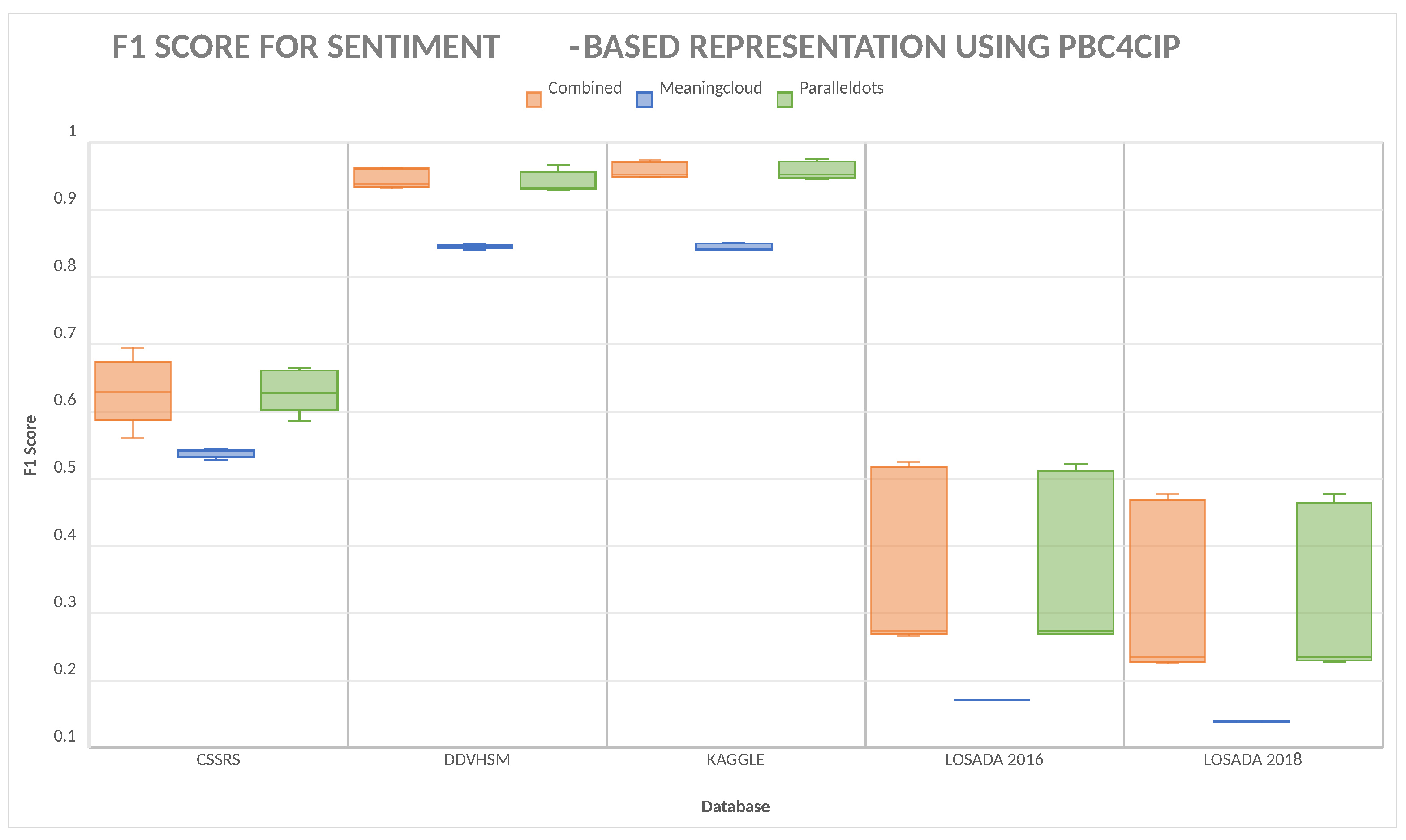
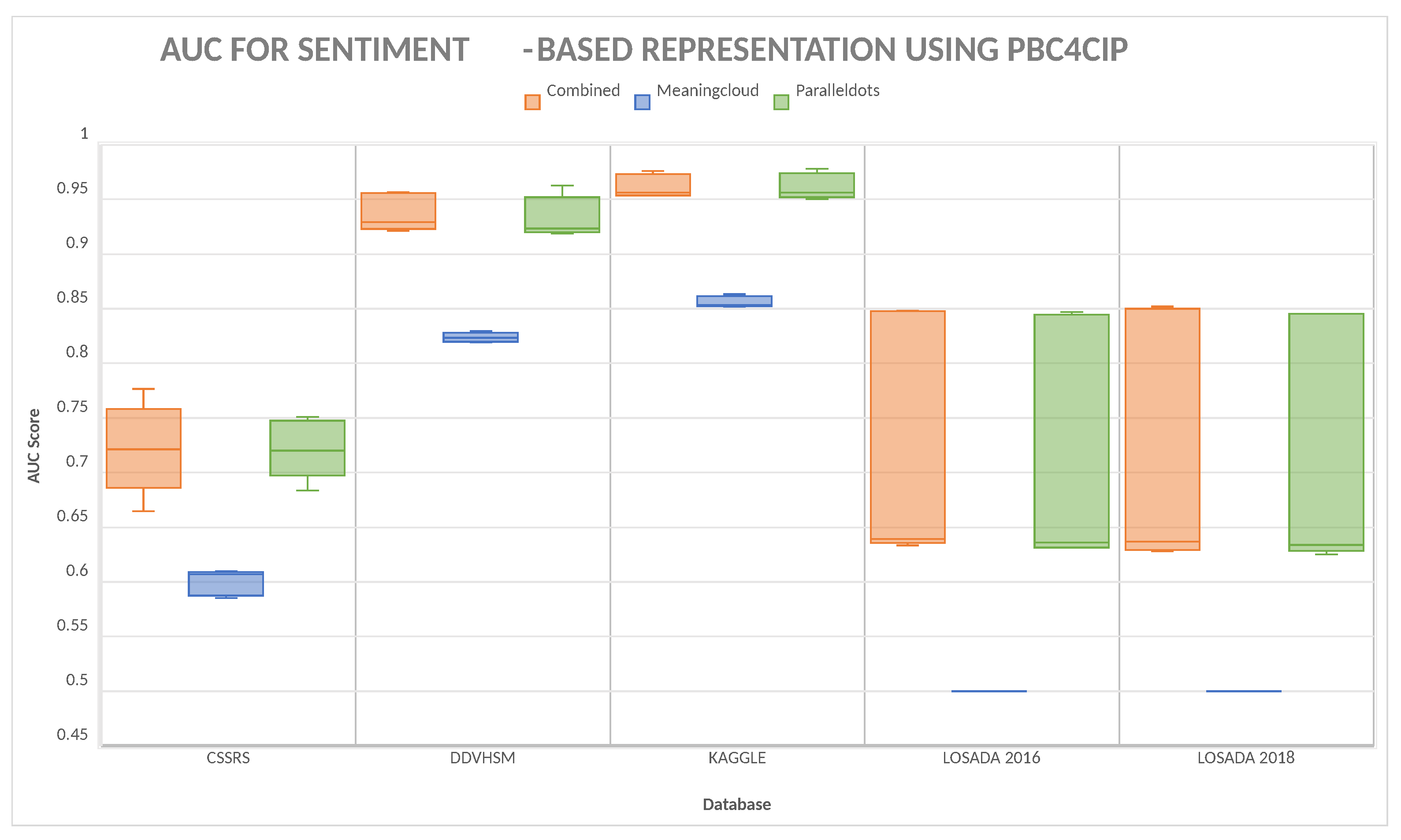
The first comparison we performed was between the three different representations proposed in this paper. As seen in Figure 2 and Figure 3, the worst performing representation is Meaningcloud in both metrics. This representation allows obtaining an average F1 score of 0.5076, having the best performance with the database of Kaggle with an average performance of 0.8459. The worst performance of this metric was with the LOSADA2018 database with an average performance of 0.1390. For the AUC, the worst performance is given by the Meaningcloud representation, having its best average performance of 0.8562 with Kaggle and its worst average performance of 0.5 with LOSADA2018; the predictions were not better than random predictions.

On the other hand, the best F1 performance was achieved by the combined representation with an average performance of 0.6457 taking into consideration all the databases. The best performance is with the database Kaggle with an average performance of 0.9586. The representation that gives the best AUC performance is again the combined representation, with its best average performance of 0.9621 with Kaggle and its worst average performance of 0.7170 with LOSADA2018.

It is important to denote that the difference between the results of the combined and Paralleldots representations has no significant difference in the F1 score, according to a Wilcoxon signed-ranks test [62], which gives a p-value of 0.1416. Nevertheless, it does present a significant difference in the AUC metric with a p-value of 0.02444.

We chose combined as the best representation, given the results, and used it as the point of comparison with other representations and classifiers.

After determining the best representation using PBC4cip, we used that representation to compare it with the results of other proposals. Since we only have results for three of the five databases using the LOSADA2016 and LOSADA2018 representation and classification technique, the results are divided into two sets. Figure 4 and Figure 5 present the comparison between our representation and the representations of LOSADA2016 and LOSADA2018 for the available databases, which are CSSRS, DDVHSM, and Kaggle. Figure 6 and Figure 7 present the comparison between our representation and the representations of Parser tree, VAD, and BOW tf-idf for all databases.

4.3. LOSADA Representations

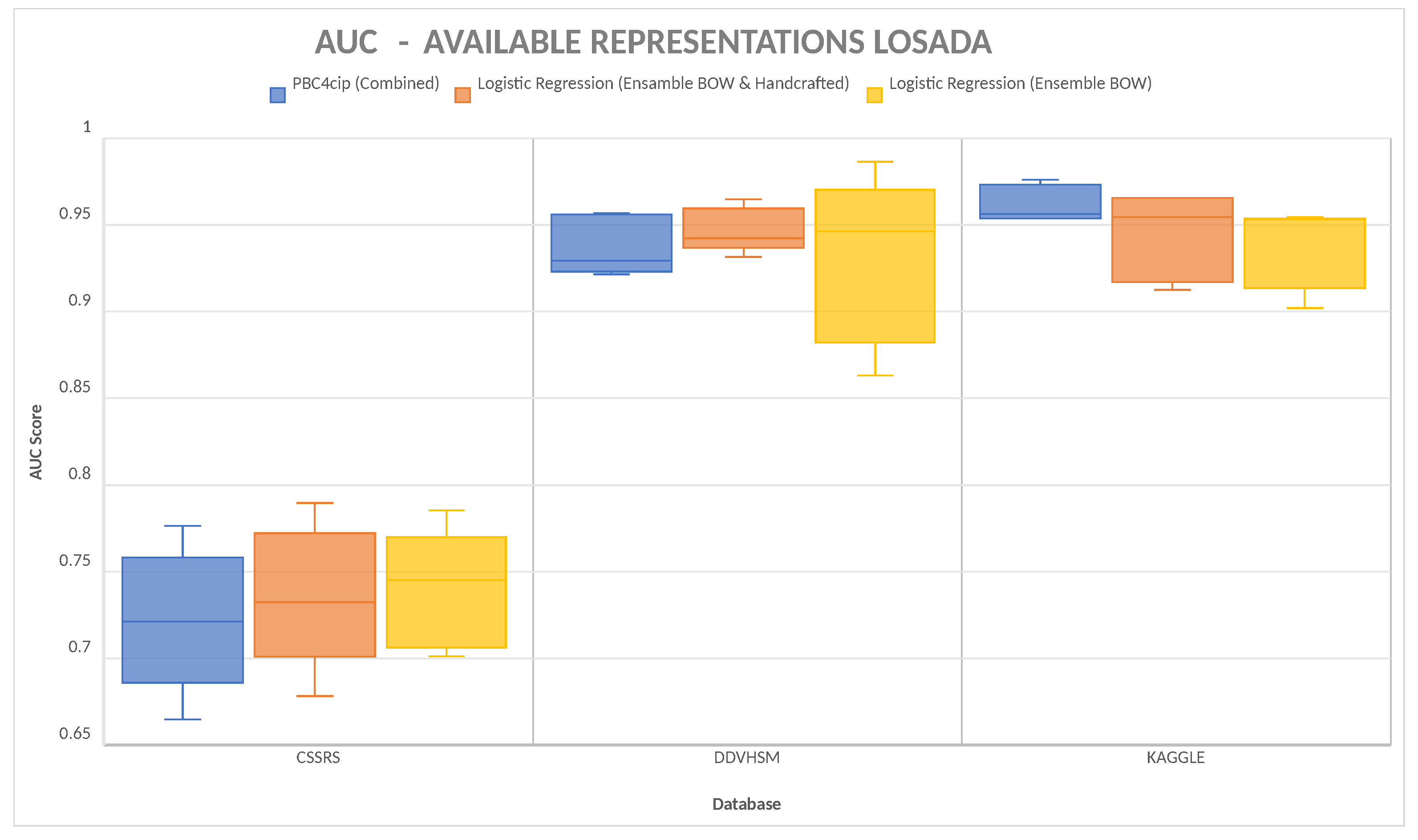
Figure 4 presents the available results of LOSADA2016 and LOSADA2018 representations. The three representation–classifier pairs perform better on the datasets DDVHSM and Kaggle and have a lower performance on CSSRS. The combined representation with PBC4cip performs better on DDVHSM and Kaggle with a mean performance of 0.9457 and 0.9586, respectively. On the other hand, the Ensemble of BOWs and Handcrafted features with logistic regression performs better on CSSRS with a mean performance of 0.6335.

As seen in Figure 5, the same pattern is repeated when using AUC as the metric for performance. Nevertheless, using AUC, the Ensemble of BOWs and Handcrafted features with logistic regression performs better on both CSSRS and DDVHSM with a mean performance of 0.7357 and 0.9470, respectively. This contrasts with PBC4cip, which has a mean performance of 0.72191061 and 0.9375.

4.4. Other Models

As seen in Figure 6, for both LOSADA2016 and LOSADA2018 databases, the VAD representation with Naive Bayes classification presents the worst performance in F1 score. On the other hand, for the DDVHSM database, it presents the best performance. For the CSSRS and Kaggle database, the tf-idf BOW using Ada Boost classification presents the worst performance but has a better performance in the LOSADA2016 and LOSADA2018 databases. For all databases except DDVHS, the best performance is given by the sentiment-based representation with PBC4cip.

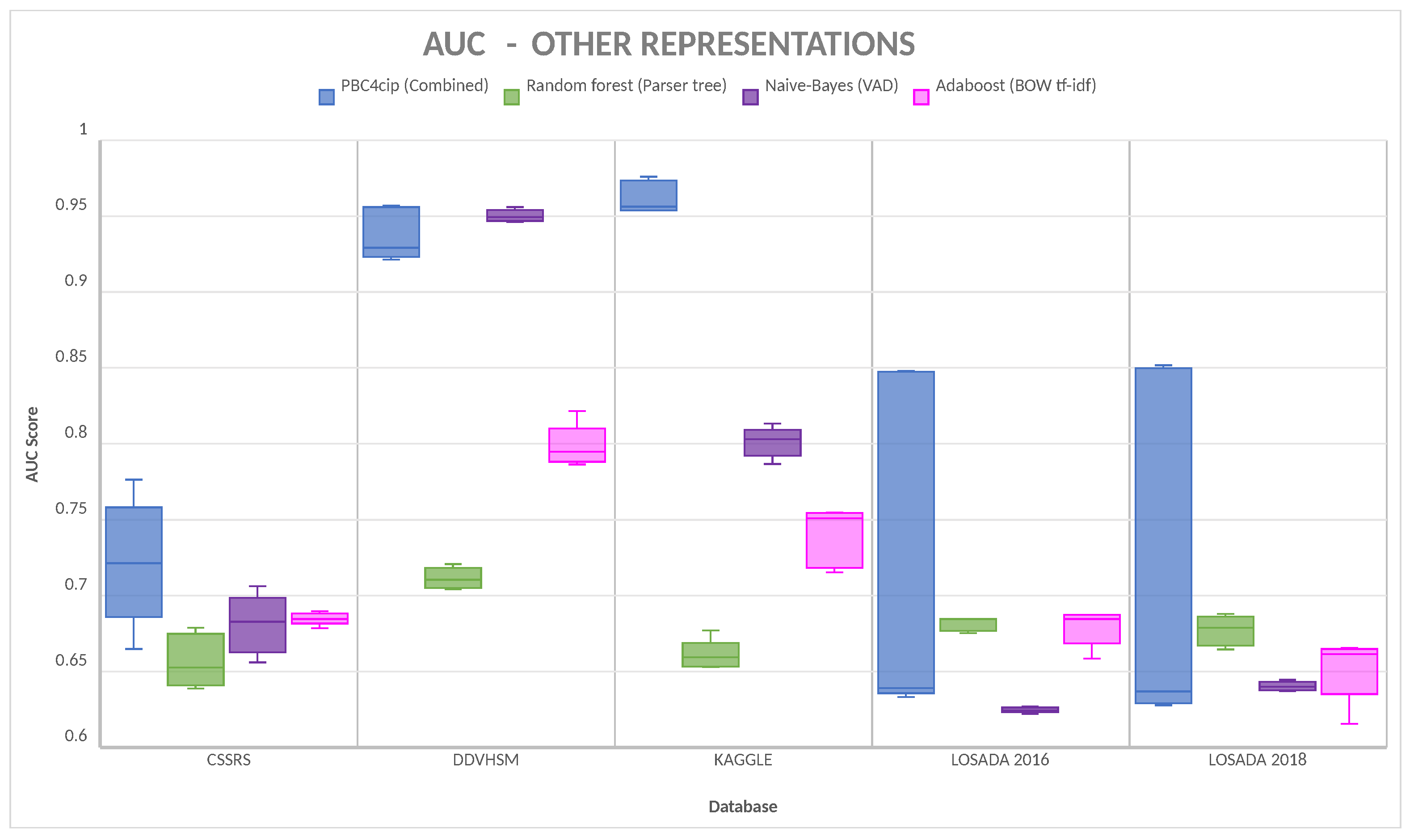
Figure 7 shows that for AUC, VAD features using Naive Bayes classification present the worst performance for LOSADA2016 and LOSADA2018. It also shows that it has a higher performance in CSSRS, DDVHSM, and Kaggle databases, having the best performance in DDVHSM. The parser tree representation with Random Forest classification presents a similar performance in all databases in comparison with its counterparts.

As we have stated before, for all databases except DDVHSM, the best performance is given by sentiment-based representation with PBC4cip.

4.5. Wilcoxon Test

After obtaining and visually comparing the results, we performed a Wilcoxon signed-ranks test [62] to assess whether there is a significant difference between the results of the different classifiers or not. We used this test because it is recommended in cases where the same models or subjects are assessed under more than one different condition. It is also recommended when what is being assessed is the definite numeric scores instead of nominal values [63].

The Wilcoxon signed rank test has a null hypothesis $H_0:M_1=M_2$ and an alternative hypothesis $H_1:M_1\ne M_2$, where $M_1$ and $M_2$ are the datasets that are being compared. We first have to subtract the values of one dataset from the other dataset, that is, $D=M_1-M2$. After that, we have to rank the absolute values of D in ascending order, that is, the smallest value of $\left|D\right|$ is number 1, and the highest value of $\left|D\right|$ is number n, where n is the number of values in the datasets.

We then add all the positive values of D obtaining $T_{+}$ and all the negative values of D obtaining $T_{-}$. We obtain the Wilcoxon statistic using the following formula:

$$W_{stat}=min(T_{-},T_{+})$$

We obtain the Wilcoxon critical value $W_{crit}$ using the Wilcoxon signed-ranked test quantiles table. After that, we compare $W_{crit}$ and $W_{stat}$. If $W_{stat}<W_{crit}$, then we reject the null hypothesis, meaning that there is a statistical difference between the datasets. On the other hand, if $W_{stat}>W_{crit}$, we accept the null hypothesis, meaning that there is no statistical difference between the datasets.

Table 7. Mean F1 and AUC scores for each model tested.

Model	Database	Scores
		F1	AUC
Logistic Regression (Ensemble BOW and Handcrafted)	CSRRS	0.6335	0.7357
	DDVHSM	0.9433	0.9470
	Kaggle	0.9428	0.9438
Logistic Regression (Ensemble BOW)	CSRRS	0.6469	0.7395
	DDVHSM	0.9026	0.9302
	Kaggle	0.9236	0.9376
Random Forest (parser-tree)	CSRRS	0.5231	0.6568
	DDVHSM	0.7611	0.7115
	Kaggle	0.6149	0.6606
	LOSADA2016	0.2797	0.6815
	LOSADA2018	0.2545	0.6771
Naive-Bayes (VAD and Topics)	CSRRS	0.5740	0.6810
	DDVHSM	0.9553	0.9502
	Kaggle	0.7853	0.8011
	LOSADA2016	0.2392	0.6247
	LOSADA2018	0.2097	0.6404
AdaBoost (BOW)	CSRRS	0.3218	0.6848
	DDVHSM	0.7893	0.7983
	Kaggle	0.5371	0.7392
	LOSADA2016	0.3505	0.6793
	LOSADA2018	0.2585	0.6523
PBC4-cip (combined)	CSRRS	0.6298	0.7219
	DDVHSM	0.9457	0.9375
	Kaggle	0.9586	0.9621
	LOSADA2016	0.3694	0.7212
	LOSADA2018	0.3250	0.7190

shows the mean of the scores obtained by each model per database. The values used for the Wilcoxon test were the results obtained per partition, for each database.

Table 8. Wilcoxon signed-ranks test, comparing the classification results of our proposal against the remaining tested popular state-of-the-art proposals.

Model 1	Model 2	Measure	Sum. Pos. Ranks	Sum. Neg. Ranks	Mean Diff.	Z-Value	p-Value	Signif.
PBC4-cip (combined)	Logistic Regression (Ensemble BOW and Handcrafted)	F1	62	58	0.19	−0.1136	0.9124	No
		AUC	54	66	0.08	−0.3408	0.7279	No
	Logistic Regression (Ensemble BOW)	F1	94	26	0.19	−1.9311	0.0536	No
		AUC	67	53	0.13	−0.3976	0.6892	No
	Random Forest (parser-tree)	F1	305	20	0.08	−3.8342	0.0001	Yes
		AUC	296	29	0.13	−3.5921	0.0003	Yes
	Naive-Bayes (VAD and Topics)	F1	301	24	0.11	−3.7266	0.0002	Yes
		AUC	261	64	0.16	−2.6503	0.0080	Yes
	AdaBoost (BOW)	F1	215	110	0.04	−1.4126	0.1585	No
		AUC	127	108	0.1	−1.4664	0.1416	No

shows the results obtained from the test. When comparing the models, we could see that the logistic regression classifier together with the Ensemble of BOWs and Handcrafted features performed better on some databases. Nevertheless, according to the Wilcoxon test performed, there is no significant difference between the F1 score and AUC of the sentiment-based representation together with PBC4cip. The results also show that there are classifiers and representations with which there is a significant difference. However, the difference proves an advantage of using sentiment-features with PBC4cip over the other classifiers. Moreover, PBC4cip provided patterns that explain the decisions taken by the classifiers. The features that are taken more into consideration by the model to classify a social media post as depressive or not depressive are as follows:

• The emotions of sadness, excitement, anger, and boredom in the text.
• The polarity of the text, especially whether the text is neutral or not.
• The subjectivity of the text.

5. Interpretation of Patterns

Table 9. Example of contrast patterns obtained, showing the support for depressed and not depressed posts.

ID	Pattern	Support
		Depressive	Not Depressive
$P_1$	Sad > 0.14 & Excited ≤ 0.08 & Angry > 0.02 & Polarity ≠ ’P’ & Bored ≤ 0.72 & Happy ≤ 0.05	0.4	0
$P_2$	Abusive > 0.49 & Positive ≤ 0.23 & Excited ≤ 0.16 & Negative > 0.66 & Happy ≤ 0.05	0.32	0
$P_3$	Happy ≤ 0.09 & Positive ≤ 0.30 & Polarity ≠ ’NONE’ & Sad > 0.03 & Complaint > 0.44 & Hate_Speech ≤ 0.01	0.3	0
$P_4$	Marketing ≤ 0.01 & Polarity ≠ ’P’ & Positive ≤ 0.18 & Abusive > 0.92 & Happy ≤ 0.05	0.29	0
$P_5$	Sad > 0.14 & Complaint > 0.19 & Query ≤ 0.20 & Neutral ≤ 0.33 & Spam ≤ 0.43 & Happy ≤ 0.09	0.29	0
$P_6$	Positive ≤ 0.27 & Neither ≤ 0.54 & Happy ≤ 0.07	0.29	0
$P_7$	Complaint > 0.42 & Happy ≤ 0.07 & Polarity ≠ ’NONE’ & Hate_Speech ≤ 0.01	0.29	0
$P_8$	Positive ≤ 0.24 & Marketing ≤ 0.01 & Negative > 0.60 & Excited ≤ 0.03	0.28	0
$P_9$	Neutral > 0.46 & Not-Sarcastic ≤ 0.73 & Sarcastic > 0.29 & Negative ≤ 0.26	0	0.21
$P_{10}$	Sad ≤ 0.29 & Polarity ≠ ’NEU’ & News ≤ 0.28 & Negative ≤ 0.22 & Query ≤ 0.17 & Excited ≤ 0.42	0	0.21

shows examples of the contrast patterns obtained by the model, as well as their support for the depressive and non-depressive class. These patterns can be interpreted in natural language, this interpretation can be found in

Table 10. Explanation in natural language of example patterns in Table 9.

ID	Interpretation in Natural Language of Extracted Patterns
$P_1$	Depressive posts have at least a minimum amount of sadness and anger, almost no excitement or happiness, a polarity that is either negative or neutral, and up to a medium high level of boredom.
$P_2$	Depressive posts have at least a medium high level of negativity and a medium low level of abusive content, at most a low level of positivity, and almost no excitement or happiness.
$P_3$	Depressive posts have almost no happiness or hate speech, at most a low level of positivity, a polarity that is either positive or negative, at least a minimum amount of sadness and at least a medium-low level of complaints.
$P_4$	Depressive posts have almost no intent of marketing, positivity, or happiness, a polarity that is either negative or neutral and at least a high level of abusive content.
$P_5$	Depressive posts have at least a minimum amount of sadness and complaints, at most a medium low level of intent of spam and neutrality, at most a medium low level of query intent, and almost no happiness.
$P_6$	Depressive posts have at most a low level of positivity and a medium level of not-abusive and not-hate-speech content, and almost no happiness.
$P_7$	Depressive posts have at least a medium-low level of complaints, a polarity that is either positive or negative, and almost no happiness or hate-speech content.
$P_8$	Depressive posts have at most a low level of positivity, almost no intent of marketing or excitement, and at least a medium-high level of negativity.
$P_9$	Not depressive posts have at least a medium low level of neutrality and a low level of sarcasm, and at most a medium-high level of not-sarcastic content and a low level of negativity.
$P_{10}$	Not depressive posts have at most a low level of sadness, negativity, and intent of news or query, a polarity either positive or negative, and at most a medium-low level of excitement.

.

Patterns show that depressive tweets tend to have a higher probability of containing text representing sadness, anger and boredom and a lower probability of containing text representing excitement, happiness, or a positive polarity. Moreover, depressive posts can be identified by the lack of excitement and happiness more than by the presence of sadness or anger. The contrast patterns obtained show that for 40% of depressive posts, and over 0% of the non-depressive posts, the feelings of excitement and happiness do not go higher than 0.05. On the other hand, the levels of sadness, anger and boredom can vary from 0.02 upwards. Polarity is also important, as positive polarity is linked to 65% of the non-depressive posts and only 20% of the depressive posts. Nevertheless, neutral polarity is linked to both depressive and non-depressive posts. The patterns also showed that non-depressive posts contain more sarcasm (a probability higher than 0.52) than depressive posts. In addition, the posts are objective for 26% of the depressive posts in contrast with 0% of the non-depressive posts.

6. Conclusions and Future Work

Depression detection has become an essential task, as it has multiple risks to individuals, society, and economics. Due to the lack of specialists per patients, this task has become difficult and has escalated, becoming a global problem. Since there is a link between language and signs of depression, social media is used to detect depression, using users’ posts. The literature shows that most of these solutions provide a representation of text using objective features, such as the number of pronouns, the count of a certain word, or the use of certain phrases inside the text.

However, as far as we know, state-of-the-art proposals do not provide their result in a language close to the human expert, which is essential for helping decision makers in the application area. Hence, in this paper, we proposed a new representation of the text based on sentiment analysis and emotions to provide an understandable representation, allowing to discriminate depressive and non-depressive posts in a language close to that of human experts. The aim was to provide experts the information of social media to aid in the diagnosis of users, who may not know they have depression. We also proposed an understandable model based on our representation and pattern-based classification, obtaining both an understandable and accurate model for human experts.

Our proposed model outperforms most of the other five state-of-the-art models for depression detection. Additionally, it provides insights on the sentiment-features that define a depressive or a non-depressive post, providing more information to an expert or even the posts’ author. Moreover, based on the statistical tests and F1 and AUC metrics, our model statistically outperforms the Random Forest, Naive Bayes, and AdaBoost models using the parser-tree, VAD and Topics, and BOW representations. However, it obtains similar statistical results to the logistic regression models, using the ensemble of BOWs and handcrafted features representations. Consequently, we can conclude that our proposed model, as well as the representation based on sentiments and emotions, allows for providing the best classification results for predicting depressive posts.

In future work, we plan on exploring new representations, including features directly related to the medical symptoms of depression and fuzzy pattern classification. The assessment of psychology experts on the patterns and the subsequent interpretation is also part of our future work on this topic.

References

1. Roberts, N.L.; Mountjoy-Venning, W.C.; Anjomshoa, M.; Banoub, J.A.M.; Yasin, Y.J. Global, regional, and national incidence, prevalence, and years lived with disability for 354 diseases and injuries for 195 countries and territories, 1990–2017: A systematic analysis for the Global Burden of Disease Study. Lancet 2018, 392, 1789–1858. [Google Scholar]
2. World Health Organization. Depression and Other Common Mental Disorders: Global Health Estimates; Technical Report; World Health Organization: Geneva, Switzerland, 2017. [Google Scholar]
3. Jenkins, R.; Baingana, F.; Ahmad, R.; McDaid, D.; Atun, R. Social, economic, human rights and political challenges to global mental health. Ment. Health Fam. Med. 2011, 8, 87. [Google Scholar] [PubMed]
4. World Health Organization. Mental Health Action Plan 2013–2020; WHO Document Production Services: Geneva, Switzerland, 2013. [Google Scholar]
5. American Psychiatric Association. Diagnostic and Statistical Manual of Mental Disorders (DSM-5®); American Psychiatric Pub: Arlington, VA, USA, 2013. [Google Scholar]
6. Bloom, D.; Cafiero, E.; Jané-Llopis, E.; Abrahams-Gessel, S.; Bloom, L.; Fathima, S.; Feigl, A.; Gaziano, T.; Mowafi, M.; Pandya, A.; et al. The Global Economic Burden of Non-Communicable Diseases: A Report; World Economic Forum: Geneva, Switzerland, 2011. [Google Scholar]
7. World Health Organization. Mental Health in the Workplace. 2011. Available online: https://www.who.int/teams/mental-health-and-substance-use/mental-health-in-the-workplace (accessed on 11 October 2019).
8. World Health Organization. World Health Organization Assessment Instrument for Mental Health Systems-WHO-AIMS Version 2.2; Technical Report; World Health Organization: Geneva, Switzerland, 2005. [Google Scholar]
9. Clement. Global Digital Population 2019. Available online: https://0-www-statista-com.brum.beds.ac.uk/statistics/617136/digital-population-worldwide/ (accessed on 11 October 2019).
10. Stirman, S.W.; Pennebaker, J.W. Word Use in the Poetry of Suicidal and Nonsuicidal Poets. Psychosom. Med. 2001, 63, 517–522. [Google Scholar] [CrossRef] [PubMed]
11. Rude, S.; Gortner, E.M.; Pennebaker, J. Language use of depressed and depression-vulnerable college students. Cognit. Emot. 2004, 18, 1121–1133. [Google Scholar] [CrossRef]
12. Losada, D.E.; Crestani, F.; Parapar, J. Overview of erisk 2019 early risk prediction on the internet. In Proceedings of the International Conference of the Cross-Language Evaluation Forum for European Languages, Lugano, Switzerland, 9–12 September 2019; pp. 340–357. [Google Scholar]
13. Coppersmith, G.; Dredze, M.; Harman, C.; Hollingshead, K.; Mitchell, M. CLPsych 2015 shared task: Depression and PTSD on Twitter. In Proceedings of the 2nd Workshop on Computational Linguistics and Clinical Psychology: From Linguistic Signal to Clinical Reality, Denver, CO, USA, 5 June 2015; pp. 31–39. [Google Scholar]
14. Farıas-Anzaldúa, A.A.; Montes-y Gómez, M.; López-Monroy, A.P.; González-Gurrola, L.C. UACH-INAOE participation at eRisk2017. In Proceedings of the Conference and Labs of the Evaluation Forum CLEF, Dublin, Ireland, 11–14 September 2017; Volume 1866. [Google Scholar]
15. Malam, I.A.; Arziki, M.; Bellazrak, M.N.; Benamara, F.; El Kaidi, A.; Es-Saghir, B.; He, Z.; Housni, M.; Moriceau, V.; Mothe, J.; et al. IRIT at e-Risk. In Proceedings of the International Conference of the CLEF Association, CLEF 2017 Labs Working Notes (CLEF 2017), Dublin, Ireland, 11–14 September 2017; pp. 1–7. [Google Scholar]
16. Trotzek, M.; Koitka, S.; Friedrich, C.M. Linguistic Metadata Augmented Classifiers at the CLEF 2017 Task for Early Detection of Depression. In Proceedings of the CLEF (Working Notes), Dublin, Ireland, 11–14 September 2017. [Google Scholar]
17. Zhou, D.; Luo, J.; Silenzio, V.M.; Zhou, Y.; Hu, J.; Currier, G.; Kautz, H. Tackling Mental Health by Integrating Unobtrusive Multimodal Sensing. In Proceedings of the Twenty-Ninth AAAI Conference on Artificial Intelligence, Austin, TX, USA, 25–30 January 2015. [Google Scholar]
18. Islam, M.R.; Kamal, A.R.M.; Sultana, N.; Islam, R.; Moni, M.A.; Ulhaq, A. Detecting Depression Using K-Nearest Neighbors (KNN) Classification Technique. In Proceedings of the 2018 International Conference on Computer, Communication, Chemical, Material and Electronic Engineering (IC4ME2), Rajshahi, Bangladesh, 8–9 February 2018; pp. 1–4. [Google Scholar]
19. Jia, J. Mental Health Computing via Harvesting Social Media Data; IJCAI: Beijing, China, 2018; pp. 5677–5681. [Google Scholar]
20. Aragon, M.E.; Lopez-Monroy, A.P.; Gonzalez-Gurrola, L.C.G.; Montes, M. Detecting Mental Disorders in Social Media through Emotional Patterns-The case of Anorexia and Depression. IEEE Trans. Affect.Comput. 2021. [Google Scholar] [CrossRef]
21. Loyola-Gonzalez, O. Black-box vs. white-box: Understanding their advantages and weaknesses from a practical point of view. IEEE Access 2019, 7, 154096–154113. [Google Scholar] [CrossRef]
22. Trotzek, M.; Koitka, S.; Friedrich, C.M. Word Embeddings and Linguistic Metadata at the CLEF 2018 Tasks for Early Detection of Depression and Anorexia. In Proceedings of the CLEF (Working Notes), Avignon, France, 10–14 September 2018. [Google Scholar]
23. Losada, D.E.; Crestani, F.; Parapar, J. eRISK 2017: CLEF lab on early risk prediction on the internet: Experimental foundations. In Proceedings of the International Conference of the Cross-Language Evaluation Forum for European Languages, Dublin, Ireland, 11–14 September 2017; pp. 346–360. [Google Scholar]
24. Villegas, M.P.; Funez, D.G.; Ucelay, M.J.G.; Cagnina, L.C.; Errecalde, M.L. LIDIC-UNSL’s Participation at eRisk 2017: Pilot Task on Early Detection of Depression. In Proceedings of the CLEF (Working Notes), Dublin, Ireland, 11–14 September 2017. [Google Scholar]
25. Tausczik, Y.R.; Pennebaker, J.W. The Psychological Meaning of Words: LIWC and Computerized Text Analysis Methods. J. Lang. Soc. Psychol. 2010, 29, 24–54. [Google Scholar] [CrossRef]
26. Errecalde, M.L.; Villegas, M.P.; Funez, D.G.; Ucelay, M.J.G.; Cagnina, L.C. Temporal Variation of Terms as Concept Space for Early Risk Prediction. In Proceedings of the CLEF (Working Notes), Dublin, Ireland, 11–14 September 2017. [Google Scholar]
27. Cambria, E.; Olsher, D.; Rajagopal, D. SenticNet 3: A common and common-sense knowledge base for cognition-driven sentiment analysis. In Proceedings of the AAAI Conference on Artificial Intelligence, Québec City, QC, Canada, 27–31 July 2014; Volume 28. [Google Scholar]
28. Almeida, H.; Briand, A.; Meurs, M.J. Detecting Early Risk of Depression from Social Media User-generated Content. In Proceedings of the CLEF (Working Notes), Dublin, Ireland, 11–14 September 2017. [Google Scholar]
29. Giannakopoulos, G.; Mavridi, P.; Paliouras, G.; Papadakis, G.; Tserpes, K. Representation models for text classification: A comparative analysis over three web document types. In Proceedings of the 2nd International Conference on Web Intelligence, Mining and Semantics, Craiova, Romania, 13–15 June 2012; pp. 1–12. [Google Scholar]
30. Villatoro-Tello, E.; Ramírez-de-la Rosa, G.; Jiménez-Salazar, H. UAM’s Participation at CLEF eRisk 2017 task: Towards Modelling Depressed Blogers. In Proceedings of the CLEF (Working Notes), Dublin, Ireland, 11–14 September 2017. [Google Scholar]
31. Go, A.; Bhayani, R.; Huang, L. Sentiment 140 API. Available online: http://help.sentiment140.com/api (accessed on 2 December 2020).
32. Yuan, J.; Mcdonough, S.; You, Q.; Luo, J. Sentribute: Image Sentiment Analysis from a Mid-level Perspective. In Proceedings of the Second International Workshop on Issues of Sentiment Discovery and Opinion Mining, Chicago, IL, USA, 11 August 2013; pp. 1–8. [Google Scholar]
33. Mohammad, S.M.; Turney, P.D. Crowdsourcing a Word-emotion Association Lexicon. Comput. Intell. 2013, 29, 436–465. [Google Scholar] [CrossRef] [Green Version]
34. Park, M.; Cha, C.; Cha, M. Depressive moods of users portrayed in Twitter. In Proceedings of the ACM SIGKDD Workshop on Healthcare Informatics, Beijing, China, 12 August 2012; pp. 1–8. [Google Scholar]
35. Farseev, A.; Samborskii, I.; Chua, T.S. bBridge: A Big Data Platform for Social Multimedia Analytics. In Proceedings of the 24th ACM International Conference on Multimedia, Amsterdam, The Netherlands, 15–19 October 2016; pp. 759–761. [Google Scholar]
36. Gaur, M.; Alambo, A.; Sain, J.P.; Kursuncu, U.; Thirunarayan, K.; Kavuluru, R.; Sheth, A.; Welton, R.; Pathak, J. Knowledge-aware assessment of severity of suicide risk for early intervention. In Proceedings of the World Wide Web Conference, San Francisco, CA, USA, 13–17 May 2019; pp. 514–525. [Google Scholar]
37. Shen, G.; Jia, J.; Nie, L.; Feng, F.; Zhang, C.; Hu, T.; Chua, T.S.; Zhu, W. Depression Detection via Harvesting Social Media: A Multimodal Dictionary Learning Solution; IJCAI: Melbourne, Australia, 2017; pp. 3838–3844. [Google Scholar]
38. Fiorela. Data_Depression. 2020. Available online: https://www.kaggle.com/fiorela/data-depresion (accessed on 11 January 2020).
39. Losada, D.E.; Crestani, F. A test collection for research on depression and language use. In Proceedings of the International Conference of the Cross-Language Evaluation Forum for European Languages, Évora, Portugal, 5–8 September 2016; pp. 28–39. [Google Scholar]
40. Losada, D.E.; Crestani, F.; Parapar, J. Overview of eRisk: Early risk prediction on the internet. In Proceedings of the International Conference of the Cross-Language Evaluation Forum for European Languages, Avignon, France, 10–14 September 2018; pp. 343–361. [Google Scholar]
41. Meaningcloud. Meaningcloud Sentiment Analysis API. Available online: https://www.meaningcloud.com/developer/sentiment-analysis/doc/2.1 (accessed on 11 January 2020).
42. Paralleldots. Paralleldots AI Powered Text Analysis APIs. Available online: https://apis.paralleldots.com/text_docs/index.html (accessed on 11 January 2020).
43. Ekman, P. Basic emotions. Handb. Cognit. Emot. 1999, 98, 16. [Google Scholar]
44. Loyola-González, O.; Medina-Pérez, M.A.; Martínez-Trinidad, J.F.; Carrasco-Ochoa, J.A.; Monroy, R.; García-Borroto, M. PBC4cip: A new contrast pattern-based classifier for class imbalance problems. Knowl.-Based Syst. 2017, 115, 100–109. [Google Scholar] [CrossRef]
45. Loyola-González, O.; Monroy, R.; Rodríguez, J.; López-Cuevas, A.; Mata-Sánchez, J.I. Contrast pattern-based classification for bot detection on twitter. IEEE Access 2019, 7, 45800–45817. [Google Scholar] [CrossRef]
46. Chen, L.; Dong, G. Using Emerging Patterns in Outlier and Rare-Class Prediction. In Contrast Data Mining: Concepts, Algorithms, and Applications; Chapman and Hall/CRC: Boca Raton, FL, USA, 2013. [Google Scholar]
47. Kobylinski, L.; Walczak, K. Emerging Patterns and Classification for Spatial and Image Data. In Contrast Data Mining: Concepts, Algorithms, and Applications; Chapman and Hall/CRC: Boca Raton, FL, USA, 2013. [Google Scholar]
48. Li, J.; Wong, L. Emerging pattern based rules characterizing subtypes of leukemia. In Contrast Data Mining: Concepts, Algorithms, and Applications; Chapman and Hall/CRC: Boca Raton, FL, USA, 2013. [Google Scholar]
49. Davatzikos, C.; Fan, Y.; Wu, X.; Shen, D.; Resnick, S.M. Detection of prodromal Alzheimer’s disease via pattern classification of magnetic resonance imaging. Neurobiol. Aging 2008, 29, 514–523. [Google Scholar] [CrossRef] [PubMed] [Green Version]
50. Wei, W.; Li, J.; Cao, L.; Ou, Y.; Chen, J. Effective detection of sophisticated online banking fraud on extremely imbalanced data. World Wide Web 2013, 16, 449–475. [Google Scholar] [CrossRef]
51. Zhang, X.; Dong, G. Overview and Analysis of Contrast Pattern-Based Classification. In Contrast Data Mining: Concepts, Algorithms, and Applications; Chapman and Hall/CRC: Boca Raton, FL, USA, 2013. [Google Scholar]
52. Cañete-Sifuentes, L.; Monroy, R.; Medina-Pérez, M.A.; Loyola-González, O.; Voronisky, F.V. Classification based on multivariate contrast patterns. IEEE Access 2019, 7, 55744–55762. [Google Scholar] [CrossRef]
53. Hernández, V.A.S.; Monroy, R.; Medina-Pérez, M.A.; Loyola-González, O.; Herrera, F. A Practical Tutorial for Decision Tree Induction: Evaluation Measures for Candidate Splits and Opportunities. ACM Comput. Surv. (CSUR) 2021, 54, 1–38. [Google Scholar] [CrossRef]
54. Dodds, P.S.; Harris, K.D.; Kloumann, I.M.; Bliss, C.A.; Danforth, C.M. Temporal patterns of happiness and information in a global social network: Hedonometrics and Twitter. PLoS ONE 2011, 6, e26752. [Google Scholar] [CrossRef] [PubMed]
55. Manning, C.D.; Surdeanu, M.; Bauer, J.; Finkel, J.R.; Bethard, S.; McClosky, D. The Stanford CoreNLP natural language processing toolkit. In Proceedings of the 52nd Annual Meeting of the Association for Computational Linguistics: System Demonstrations, Baltimore, MD, USA, 23–24 June 2014; pp. 55–60. [Google Scholar]
56. Bradley, M.M.; Lang, P.J. Affective Norms for English Words (ANEW): Instruction Manual and Affective Ratings; Technical Report; Technical Report C-1; the Center for Research in Psychophysiology: Gainesville, FL, USA, 1999. [Google Scholar]
57. Mowery, D.; Smith, H.; Cheney, T.; Stoddard, G.; Coppersmith, G.; Bryan, C.; Conway, M. Understanding depressive symptoms and psychosocial stressors on Twitter: A corpus-based study. J. Med. Internet Res. 2017, 19, e48. [Google Scholar] [CrossRef] [PubMed]
58. Paul, S.; Jandhyala, S.K.; Basu, T. Early Detection of Signs of Anorexia and Depression Over Social Media using Effective Machine Learning Frameworks. In Proceedings of the CLEF (Working Notes), Avignon, France, 10–14 September 2018. [Google Scholar]
59. Moreno-Torres, J.G.; Sáez, J.A.; Herrera, F. Study on the impact of partition-induced dataset shift on k-fold cross-validation. IEEE Trans. Neural Netw. Learn. Syst. 2012, 23, 1304–1312. [Google Scholar] [CrossRef] [PubMed]
60. Powers, D.M. Evaluation: From Precision, Recall and F-measure to ROC, Informedness, Markedness and Correlation. arXiv 2020, arXiv:2010.16061. [Google Scholar]
61. Fawcett, T. An Introduction to ROC Analysis. Pattern Recognit. Lett. 2006, 27, 861–874. [Google Scholar] [CrossRef]
62. Wilcoxon, F. Individual comparisons by ranking methods. In Breakthroughs in Statistics; Springer: Berlin/Heidelberg, Germany, 1992; pp. 196–202. [Google Scholar]
63. Scheff, S.W. Chapter 8—Nonparametric Statistics. In Fundamental Statistical Principles for the Neurobiologist; Scheff, S.W., Ed.; Academic Press: Cambridge, MA, USA, 2016; pp. 157–182. [Google Scholar] [CrossRef] [Green Version]
Figure 1. Flowchart of the process followed to obtain the representations used in the experimentation.
Applsci 11 10932 g001
Figure 2. A comparison plot of the F1 score for the proposed sentiment-based representations using PBC4cip.
Applsci 11 10932 g002
Figure 3. A comparison plot of the AUC for the proposed sentiment-based representations using PBC4cip.
Applsci 11 10932 g003
Figure 4. A comparison plot of the F1 score for the best proposed representation using PBC4cip, and the available representations from Losada’s databases.
Applsci 11 10932 g004
Figure 5. A comparison plot of the AUC for the best proposed representation using PBC4cip, and the available representations from Losada’s databases.
Applsci 11 10932 g005
Figure 6. A comparison plot of the F1 score for the best proposed representation using PBC4cip, and other classifiers found in the literature.
Applsci 11 10932 g006
Figure 7. A comparison plot of the AUC for the best proposed representation using PBC4cip, and other classifiers found in the literature.
Applsci 11 10932 g007