An Analytic Method for Improving the Reliability of Models Based on a Histogram for Prediction of Companion Dogs’ Behaviors

Abstract

Dogs and cats tend to show their conditions and desires through their behaviors. In companion animal behavior recognition, behavior data obtained by attaching a wearable device or sensor to a dog’s body are mostly used. However, differences occur in the output values of the sensor when the dog moves violently. A tightly coupled RGB time tensor network (TRT-Net) is proposed that minimizes the loss of spatiotemporal information by reflecting the three components (x-, y-, and z-axes) of the skeleton sequences in the corresponding three channels (red, green, and blue) for the behavioral classification of dogs. This paper introduces the YouTube-C7B dataset consisting of dog behaviors in various environments. Based on a method that visualizes the Conv-layer filters in analyzable feature maps, we add reliability to the results derived by the model. We can identify the joint parts, i.e., those represented as rows of input images showing behaviors, learned by the proposed model mainly for making decisions. Finally, the performance of the proposed method is compared to those of the LSTM, GRU, and RNN models. The experimental results demonstrate that the proposed TRT-Net method classifies dog behaviors more effectively, with improved accuracy and F1 scores of 7.9% and 7.3% over conventional models.

1. Introduction

To understand the intentions of animals, it is important to identify the meaning of their behaviors. Dogs and cats, which have particularly close emotional ties and interrelationships with humans, tend to reveal their conditions and desires through their behaviors.

Conventional studies on identifying the behaviors of companion animals include studies using sensors [1,2,3,4,5] and videos [6,7]. In this paper, we describe a study conducted on the behavior identification of dogs, which, among the various types of pets, are typical companion animals. Most studies on dog behavior identification use sensor information obtained by attaching wearable or physical devices to a part of the dog’s body [1,2,3,4,5]. However, if the dog moves violently, the method of attaching the device to its body may result in the collection of data mixed with noise because differences occur in the sensor output values. As a method of replacing the sensor information, a method using visual information obtained from videos has been proposed. However, because there have been few studies on image-based behavior classification in the field of dog behavior identification, studies are conducted by supplementing such limitations based on the field of human behavior identification [8,9,10], for which many studies have been conducted. Some prior studies have used motion recognition devices, such as a Kinect, to enhance the behavior recognition rate. For example, refs. [8,9,10] used a method of identifying a person’s posture based on the joint information and depth information obtained through an RGB-D camera (e.g., Kinect). However, the method of collecting behavior data through fixed cameras may be stressful for dogs because experiments are conducted within limited spaces. Furthermore, a difficulty in modeling the dog behaviors occurs because the method limits the radius of activities of the dogs.

To resolve this problem, some researchers have proposed a method for extracting three-dimensional (3D) joint positions as a method of learning spatial and temporal information from RGB videos captured by regular cameras without a special device such as a Kinect [11,12,13]. However, this method [11,12,13] has a limitation in that it does not sufficiently express the correlation of spatiotemporal information because it delivers the joint positions of the human, which are input values, to the model by simply concatenating them. To overcome this limitation, color-based data representation methods that maintain certain vector information have emerged. However, the existing methods have a limitation in that they are optimized for audio-visual data [14] or use grayscale, which is a limited color scale for expressing 3D pose positions [15,16].

In this paper, we propose a novel but simpler data representation method using 3D skeleton sequences consisting of 2D RGB image-based joint position values (x- and y-axes) and depth information (z-axes) to identify the dog behaviors. To the best of our knowledge, this representation has not been used in the field of dog behavior recognition and has an advantage in that an efficient method of classifying dog behavior images can be applied. The models used in the prior studies introduced above cannot sufficiently represent or learn the correlations of x, y, and z axes that constitute the joints according to time because they use methods for combining skeleton sequence data through simple operations or representing them in grayscale images that have a limited number of colors. However, our proposed method can minimize the loss of spatiotemporal information because it reflects the three components (x-, y-, and z-axes) of the skeleton sequences in the corresponding three components (red, green, and blue channels) of the pixels. Furthermore, it can express the relationships of more temporal information and the spatial trajectory information of the joints through an encoding method. Moreover, it adds reliability to the derived results of the model through a method of analyzing which skeleton joints affect certain behaviors based on a Conv-layer filter visualization method. The major contributions of this study are as follows.

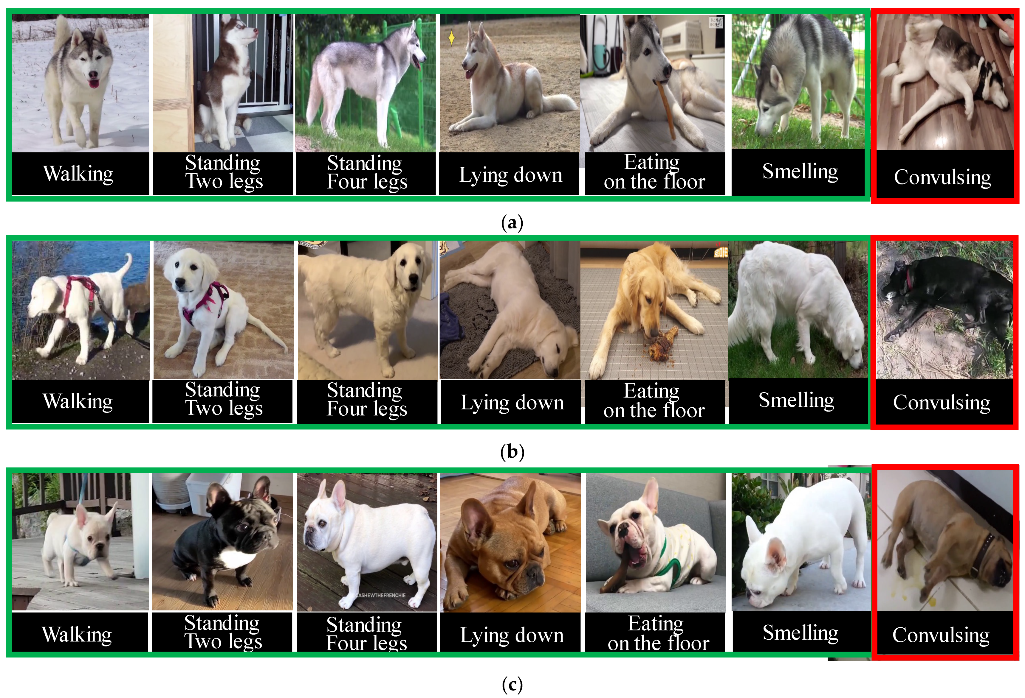
• First, this paper suggests a dog behavior dataset called the YouTube Companion Dog’s Seven Behaviors Dataset (Youtube-C7B). We collected videos containing 2D RGB image-based behavior data of dogs (French Bulldogs, Siberian Huskies, and Retrievers) from the YouTube platform. The proposed Youtube-C7B helps the behavioral modeling of dogs become more natural by collecting videos of dog behaviors in real-world environments, unlike the conventional datasets that have collected behavior data through sensors in limited spaces. Furthermore, while the conventional datasets are without labels, the dataset proposed in this study was built by labeling behaviors suitable for deep learning. Finally, in contrast to the conventional datasets, the proposed dataset contains not only normal behaviors, but also convulsing, which is an abnormal behavior, and can be used in various applications for detecting the abnormal behaviors of dogs and responding to emergency situations.
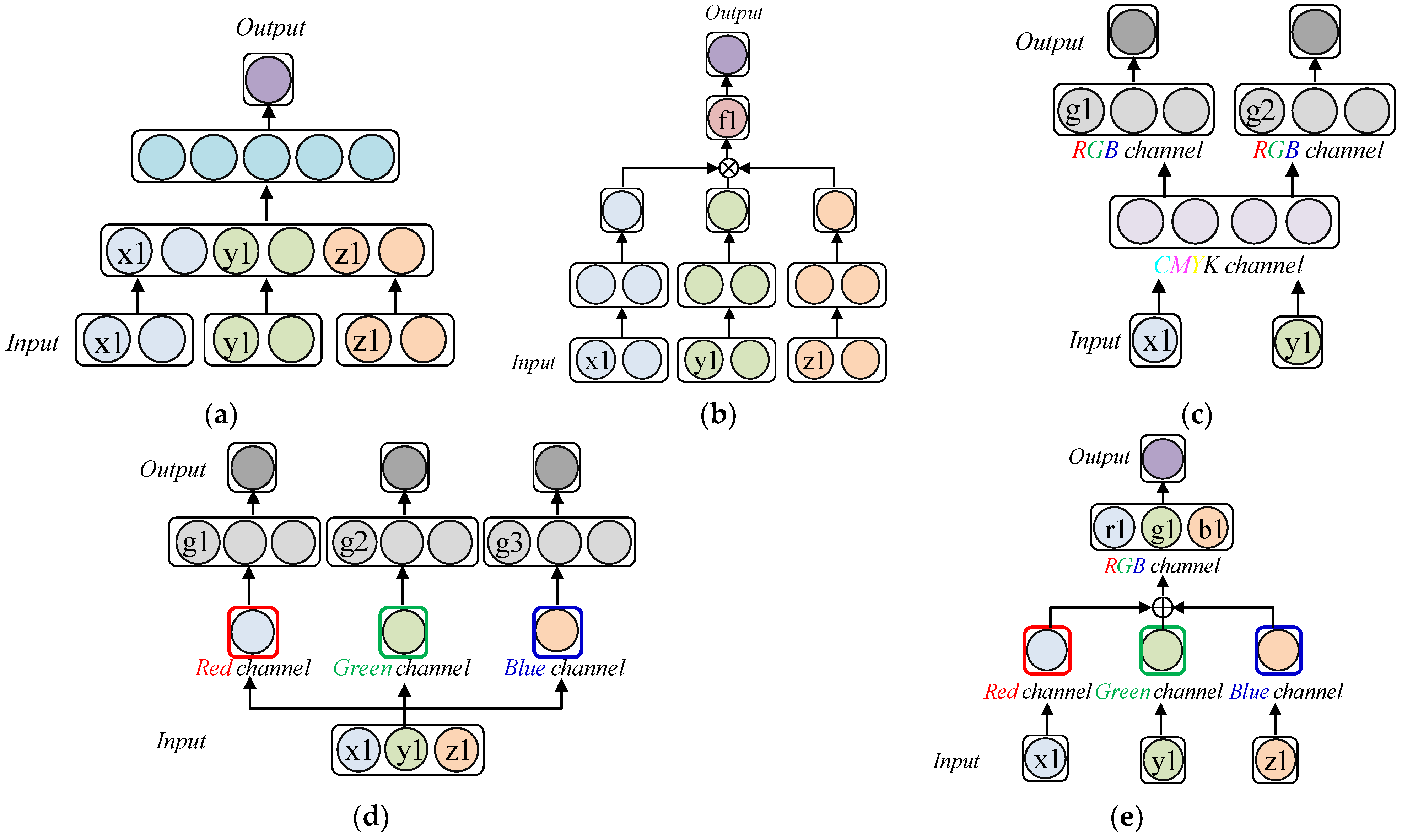
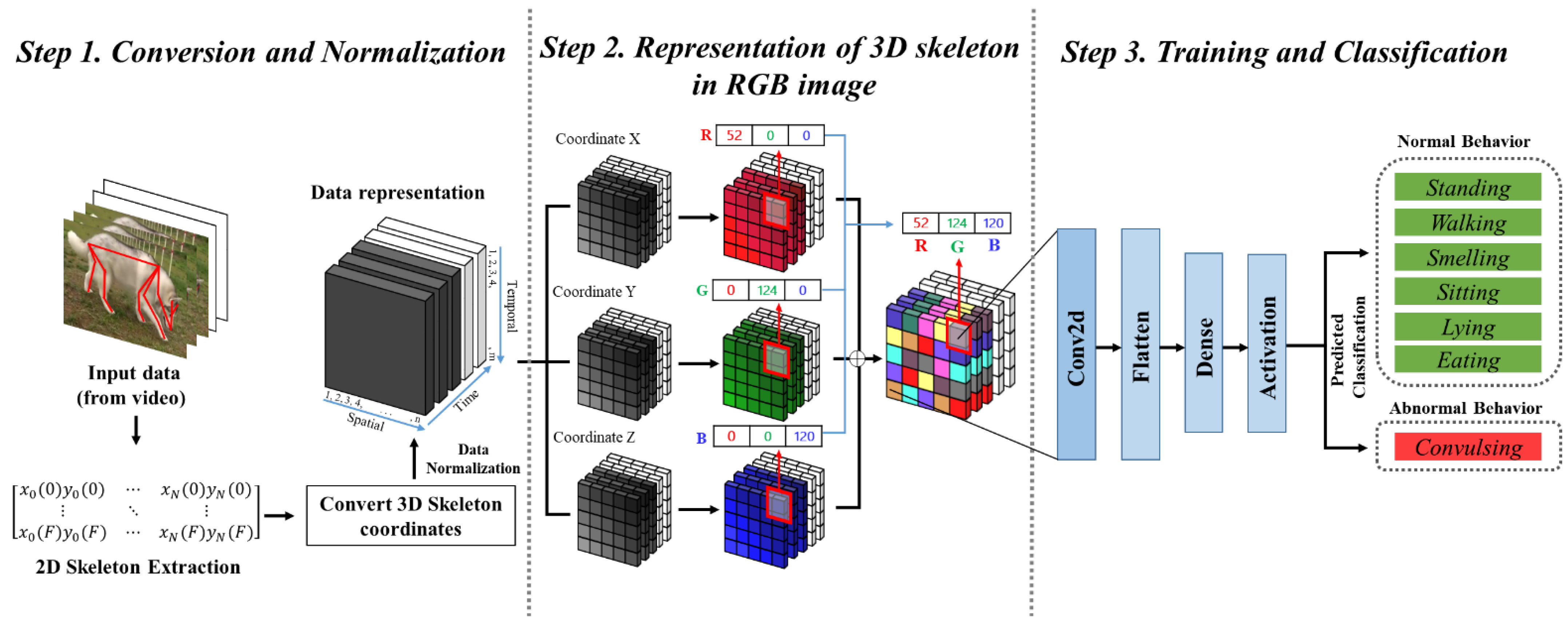
• Second, in this paper, to identify the postures of dogs, a Tightly Coupled RGB Time Tensor Network is proposed, which is an RGB-based data representation method that contains the correlations among the x-, y-, and z-axes, which change as time passes. A good representation of the changing patterns of x, y, and z over time and their relationships help to achieve a modeling with a great distance between each behavioral feature. This leads to an improved accuracy of the dog pose identification. For example, because convulsing results in more shaking on the x-, y-, and z-axes compared to standing, the patterns that change over time and their relationships should be properly represented to effectively model the dog’s behaviors. For this reason, we encode the three components (x-, y-, and z-axes) of each 3D joint position into the 3D components (red, green, and blue channels) of the RGB images and then fuse these colors. When the colors are fused in this way, it can be seen as containing the correlations of the x-, y-, and z-axes because even after fusing, it is possible to infer the pre-fusion behavior information, unlike when they were represented by vectors. Furthermore, it helps the deep learning model decode meaningful information to better identify the dog’s behaviors.
• Third, unlike conventional methods, the proposed method visualizes the filters of Conv-layer in analyzable feature maps. Thus, the patterns that the CNN memorizes for predictions can be understood. By displaying the joints extracted from the visualized feature maps based on a histogram, it is possible to know which joint part of the input image was mainly learned to make decisions.

The remainder of this paper is organized as follows. First, Section 2 introduces the trends of prior studies, and Section 3 introduces a video-based dog behavior dataset and an algorithm for the pose classification of dog behaviors using an RGB color space-based color mixing method. Section 3 also describes an algorithm that analyzes the factors affecting the derived results of the CNN model based on the analyzable feature maps. Next, Section 4 describes the experimental environment and method. Finally, Section 5 provides some concluding remarks and describes areas of future study.

2. Related Work

This section discusses relevant studies on methods for collecting behavioral posture data of dogs commonly used in the existing dog behavior recognition field and methods of behavior data representation and describes the limitations of the previous studies.

2.1. Wearable and Physical Devices for Data Collection

In the field of dog behavior research, in the past, many studies used wearable devices to enhance the accuracy of dog behavior recognition [1,2,3,4,5]. Most studies on dog behavior recognition have used physical devices such as wearables for collecting dog behavior data. For example, in [1,2,3], to obtain the position coordinates, methods are used to attach various sensors such as accelerometers, gyroscopes, and magnetometers on a harness, which is a chest strap that passes over some parts (chest, belly, back) of the dog. In [5], the authors proposed a method of recognizing behaviors by extracting the dog’s skeleton and collecting pose information through sensors placed in the clothes worn by the dog. The sensors are attached tightly to the dog’s body, helping to collect high-quality behavior data, and have the advantage of being wearable regardless of the type and size of the dog. By contrast, if the dog scratches its neck or moves violently, there is a problem in which the sensor output varies depending on the size of the dog, because the leash moves and the sensor position is not fixed.

To overcome this drawback in the sensor information collection, methods have been proposed to use visual information obtained from video sequences. For example, in [4], a method is applied for identifying the postures of a dog using a Microsoft Kinect, which does not need to be worn on the dog’s body. In addition, in [6], the authors used a method for collecting and analyzing the movements of dogs showing a propensity toward attention deficit hyperactivity disorder (ADHD) through cameras fixed to the ceiling. These methods for collecting behavior data through fixed cameras can be stressful for dogs because experiments are conducted in confined spaces. Furthermore, they have difficulty in modeling the dog behaviors because the radius of the activities of the dogs is limited.

2.2. Spaito-Temporal Data Representation

To the best of our knowledge, no studies have used spatiotemporal information based on pure video taken without sensor information in the field of dog behavior recognition and classification. Therefore, in this sub-section, we investigate the spatiotemporal data representation methods and behavior recognition models commonly used in human behavior recognition studies, which have frequently been conducted among behavior recognition studies.

Studies that obtain depth information from RGB images without depth sensors such as a Kinect have recently emerged. Furthermore, a joint-based behavior recognition method is gaining popularity, which extracts 2D joint position information based on the depth information obtained from RGB images [17]. Such 2D joint position information is important because it contains not only the joint position information but also the time sequence information. Most joint-based behavior recognition methods use recurrent neural networks (RNNs) that are suitable for time-series data processing, such as an RNN [18], an LSTM [19], and a GRU [20], to extract behaviors. For example, a hierarchical RNN [21] has been proposed, which classifies human motions based on joint position information containing spatiotemporal information; however, RNN-based methods have a limitation of overemphasizing the temporal information during training.

As a method of sufficiently learning both spatial and temporal information, a learning method of adding z-values corresponding to the depth information has been proposed. Figure 1a shows a learning method based on a data representation method that flattens the 3D joint position information over time into 1D information [11]. The late fusion method shown in Figure 1b is a learning approach that processes a variety of spatiotemporal information and joint information and fuses the resulting values during the last stage. For example, as shown in Figure 1b [12,13], tensor fusion networks that fuse the joint positions of each skeleton have been proposed. The authors proposed methods that apply various operations such as a Kronecker product and a Hadamard product, respectively, to implicitly represent spatiotemporal information and in the end fuse each feature value obtained through the operations.

As indicated above, the simple concatenation [11] and late fusion [12,13] methods have the following limitations. In Figure 1b, a new tensor called f1 is generated by fusing data through simple calculations using tensors (x1, y1, and z1) showing spatial information of each joint. However, f1 has a limitation in that it does not sufficiently represent the correlation of spatiotemporal information per frame because the feature vectors of x1, y1, and z1 before fusion are unknown.

To resolve this problem, a color-based data representation method that can maintain certain vector information was suggested. For an audio-visual tensor fusion network (AV-TFN) [14], a tensor fusion method was proposed, which represents the position information (x- and y-axes) of each joint of the skeleton and the audio information in the gray- and color scales, respectively, and fuses their colors to classify piano playing postures. The tensor fusion method proposed for AV-TFN is a color-based data representation method, which can be used to infer the pre-fusion vector information even after tensor fusion (Figure 1c). This helps the learning model learn meaningful information, such as the relationship between posture and sound. However, because AV-TFN is optimized for audio-visual data, it is unsuitable for representing the 3D poses suggested in this paper.

As a method of processing 3D posture data, the authors of [15] proposed a method of stacking gyroscope, total acceleration, and linear acceleration information row-by-row and representing them in grayscale-based images. In addition, in [16], the authors used a method of creating grayscales (g1, g2, and g3) through three channels (red, green, and blue channels) for the 3D position information (x1, y1, and z1) of the pertinent joint, as shown in Figure 1d, to integrate different spatial relationships between joints. However, the method of representing data in grayscale as above has a limited number of colors that can represent the 3D position information of the joint.

Finally, the previous methods have a problem [11,12,13,14,15,16] in that they do not provide evidence or sufficient explanation for the results derived by the model. This problem is resolved through a method of representing the RGB image, which preserves the pre-fusion data and the Conv-layer filters as analyzable feature maps (Figure 1e).

3. Tightly Coupled RGB Time Tensor Network

In this section, we introduce our new Youtube-C7B dataset (Section 3.1) and the proposed TRT-Net RGB color image-based dog behavior classification algorithm (Section 3.2).

Figure 2 shows the overall process of the TRT-Net proposed in this paper. Step 1 changes and normalizes the shape to use the dog’s 2D joint position as the input data for deep learning. To do this, it first converts the 2D joint position extracted from the video into a matrix. It then finds the z value based on the mean value of the x- and y-coordinates of each joint containing some information about the depth as z-coordinates for converting the 2D joint position into the 3D joint position [17]. The 3D joint position is as shown in the data representation diagram of Step 1. The spatial information in the data representation refers to the type of joint, and the temporal information refers to frames per second (fps). Time means the flow of time. Step 2 converts each 3D coordinate value obtained in Step 1 into the R, G, B data format. After the conversion, R, G, and B are combined into a single color and represented as a pixel. In Step 3, the model is trained to classify the dog behaviors, which are classified into normal and abnormal behaviors. Normal behaviors include standing, walking, smelling, sitting, lying, and eating, whereas convulsing corresponds to an abnormal behavior.

3.1. Creation and Selection of Behaviors

Previous studies have primarily focused on the face and body of the dog to distinguish the breeds [22,23,24,25,26]. However, there has been a lack of studies on dog behavior recognition and classification, which is the ultimate goal in the field of behavior recognition. The existing dog-related datasets are aimed at classifying breeds have been collected through sensor data in limited environments and do not include behavior labels [23,24,25,26]. Therefore, the existing dog datasets without dog behavior labels cannot be used in this study, which aims at recognizing and classifying dog behavior. In this subsection, we therefore use a method of collecting various behaviors through YouTube videos to recognize dog behaviors. To build a new Youtube-C7B dataset, the collected video images undergo processes for extracting the skeleton information and labeling the behaviors through DeepLabCut [27].

Table 1. Comparison of dataset.

Dataset Name	Year	Species	#Image	Resolution	Resource	Pose Labels	Key Points
Columbia Dogs [23]	2012	Dog	8351	Various	Flickr Image-Net Google	-	√ (Only Face)
Oxford-IIIT [24]	2012	Cat+Dog	7349	Various	Flickr Google Image-Net	-	-
Flickr-Dog [25]	2016	Dog	374	250 × 250	Flickr	-	-
Stanford Dogs [26]	2011	Dog	20,580	Various	Google	-	-
Youtube-C7B (our proposed method)	2021	Dog	10,710	Various	YouTube	√	√ (Face+Body)

compares and summarizes the properties of the Youtube-C7B dataset and dog datasets commonly used in the field of dog recognition.

Experiments were conducted on the Youtube-C7B dataset proposed in this paper by selecting the following research subjects: French Bulldogs, Retrievers, and Siberian Huskies, the behaviors of which are relatively easy to distinguish among the dogs highly preferred by people in South Korea and overseas. The Youtube-C7B dataset contains 357 behavior videos and 10,710 images collected based on YouTube videos.

We defined five daily behaviors in the Youtube-C7B dataset based on the daily behaviors of dogs defined in [3,4,28]. In this paper, we added two behaviors that were excluded from the five natural behaviors defined above. A Smelling class belonging to natural behaviors and the Convulsing class belonging to the abnormal behaviors were added. As the reason for adding the smelling behavior, dogs acquire and grasp most information through olfactory information. In other words, we added the smelling behavior of dogs as daily behaviors because smelling is an extremely important and instinctive dog behavior. The convulsing behavior was added because it pertains to one of the most common nervous system diseases occurring regardless of the dog type and size, and is caused by genetic or external factors, not infectious diseases caused by viruses or bacteria [29]. Convulsing behaviors appear as if there is some electrical shock in the brain, and a fast early response is important for the treatment of this disease. Figure 3 shows some examples of each behavior class in the dataset built in this study.

The proposed Youtube-C7B dataset has a total of seven behavior classes, i.e., six Daily classes and one Abnormal class. The Daily classes include Walking, Smelling, Standing on two legs, Standing on four legs, Lying down, and Eating off the ground, whereas the Abnormal class includes the Convulsing behavior (

Table 2. Definitions of categories in dog behavior.

Behavior	Description
Walking	Behavior of the companion dog moving to a different location when using all four legs
Standing on two Legs	Stretching the front legs straight and sitting with rear legs while the four soles are touching the ground
Standing of four legs	Posture of standing with four legs stretched straight and straightened body while the four soles are touching the ground
Lying down	Lying down with limbs either tucked under or placed in front of body
Eating off the ground	Eating food on the ground by grabbing it with front legs
Additional behavior class
Smelling	Behavior of smelling the ground, objects, or things by getting the nose close to it
Convulsing	Behavior of shaking the face and body as if an electrical shock has been applied to the brain

). Youtube-C7B includes a total of 20 key body points based on real dog skeletons. The key body points consist of two Ears, two Eyes, Nose, Throat, Withers, Tail base, four Knees, two Elbows, two Wrists, two Stifles, two Hocks, and four Paws, as shown in Figure 4.

The Youtube-C7B dataset facilitates the learning of not only the daily behavior of dogs but also abnormal behaviors because it includes dog behavior labels and the Convulsing class, unlike conventional datasets. Therefore, it offers the advantage of learning the behavioral conditions of the dogs in more detail.

3.2. Pose-Transition Feature to Image Encoding Technique

The subsections introduce TRN-Net, a new encoding technique that includes processes for feature extraction, feature arrangement, and behavior image generation.

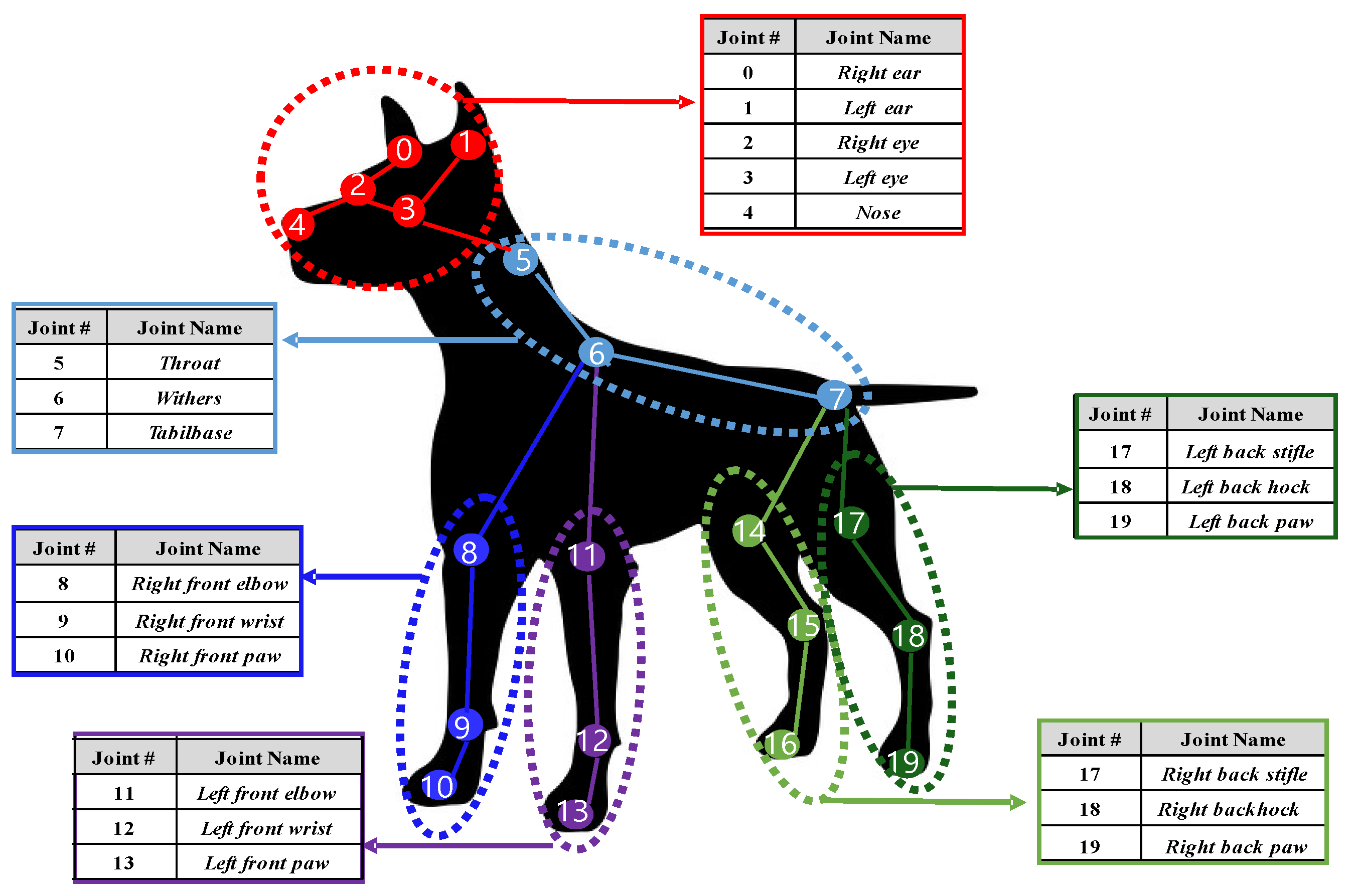
3.2.1. Pose and Transition Feature Extraction

The feature extraction stage for the dog skeleton information, which is a type of visual information, proceeds as follows. The dog’s skeleton information is extracted from the images using DeepLabCut [27] in the form of 2D coordinates (x- and y-axes). Previous dog behavior recognition studies recognized the dog’s behavior by focusing on the dog’s body. Unlike previous studies, this study adds ears and hocks and extracts the skeletons of the face (0–4), torso (5–7), and legs (8–19), as shown in Figure 4. Because dogs show emotion and behavior through their faces, including the eyes, nose, and ears, and their tails, and because their legs move the most when in motion, we extracted the face and legs by dividing them in more detail than in previous studies [5,7].

A good representation of the changes in the patterns of x, y, and z over time as well as their relationships helps in conducting modeling with a long distance between each behavioral feature. Furthermore, this leads to an improved accuracy of the dog pose identification.

3.2.2. Behavior Image Generation (RGB Color Encoding)

To represent the correlations among x, y, and z corresponding to the 3D dog pose coordinates, it is important to preserve the identity of each data item even if the data are fused [14]. In this study, we represent the data by using the RGB color space to preserve the identity of the data, unlike conventional methods that digitalize data in a 2D or 3D data structure. In the RGB color space, colors are represented using the “additive color mixing method,” in which the brightness (value) increases when colors are mixed. This is characterized by the ability to represent more various colors through the hue, saturation, and value (HSV), the three properties of color. RGB color encoding of a 3D form solves the problem that the feature vectors of the data before fusion cannot be estimated in conventional methods, which train models by simply multiplying feature values.

Algorithm 1 shows an overall process to represent the correlation between the dog’s behavior data in RGB color–space-based images.

Table 3. Summary of notation.

Symbols	Definition
$t$	Mean frame per second $\left(0\le t\le 30\right)$
n	Number of skeleton joints
$V$	Extracted skeleton coordinate from videos
$VT$	Conversion visual tensor
pixRGB	RGB color pixels
$imgRGB$	Color visual tensor image
$R$	Red channel in RGB
$G$	Green channel in RGB
B	Blue channel in RGB

shows the major notations used in Algorithm 1, which is conducted in the three steps described below.

Algorithm 1: Construct RGB-color based Video Tensor

Input:$Extractedskeletonvaluesfromvideos$ Output:$Thelistofrgb-colorvisualtensor$

Step 1. Conversion and Normalization (Lines 1–8). It is extremely important to convert skeleton joint sequences while keeping the temporal–spatial information intact [30]. In this study, we represent data through a method in which the skeleton joints of the dog are represented in rows, and each frame in a column is based on the method described in [31]. A total of 20 2D joints (two ears, two eyes, nose, throat, withers, tail base, two elbows, two wrists, two stifles, two hocks, and four paws) of a dog are extracted from each frame. The 2D joint coordinates $p\left(x_n,y_n\right)$ of the dog extracted from each frame are converted into 3D joint coordinates $p\left(x_n,y_n,z_n\right)$, in which the depth information has been added. Here, as shown in line 7, the z-coordinate showing the depth information is represented through the mean value of the x- and y-coordinates that have the depth information [17]. Equation (1) shows the formula for finding the z-coordinate value.

$$z_i\left(f\right)=MEAN\Vert (p\left(x_i,y_i\right)\Vert$$

(1)

Here, S(Skel(f)) represents the skeleton sequence of a dog, and $Skel\left(f\right)=Ske{l}_0\left(f\right),Ske{l}_1\left(f\right),\dots ,Ske{l}_m\left(f\right)$ represents the set of the skeleton joint positions. Here, the number of joints $n=0,1,\dots ,N$, the number of frames $f=0, 1, 2,\dots ,F$, and $Ske{l}_n=p\left(x_n,y_n,z_n\right), \forall p\left(x_n,y_n,z_n\right)\in {ℝ}^3$. In addition, S(Skel(f)) can be represented in the following matrix form:

$$S\left(Skel\left(f\right)\right)=\left(\begin{array}{ccc}{x}_0\left(0\right)y_0\left(0\right)z_0\left(0\right)& \cdots & x_N\left(0\right)y_N\left(0\right)z_N\left(0\right)\\ ⋮& \ddots & ⋮\\ x_0\left(F\right)y_0\left(F\right)z_0\left(F\right)& \cdots & x_N\left(F\right)y_N\left(F\right)z_N\left(F\right)\end{array}\right)$$

The joint position values of each joint of S(Skel(f)) are extracted by dividing into $x_n\left(f\right), y_n\left(f\right), z_n\left(f\right)$, and the extracted $x_n\left(f\right), y_n\left(f\right), z_n\left(f\right)$ are put into X, Y, and Z in a list form again. Here, S(Skel(f)) is redefined as S(Skel(f)) = [X, Y, Z], where X, Y, and Z have the following tensor matrixes:

$$X=\left(\begin{array}{ccc}{x}_0\left(0\right),x_1\left(0\right)& \cdots & x_{N-1}\left(0\right),x_N\left(0\right)\\ ⋮& \ddots & ⋮\\ x_0\left(F\right),x_1\left(F\right)& \cdots & x_{N-1}\left(F\right),x_N\left(F\right)\end{array}\right)$$

$$Y=\left(\begin{array}{ccc}{y}_0\left(0\right),y_1\left(1\right)& \cdots & y_{N-1}\left(0\right),y_N\left(0\right)\\ ⋮& \ddots & ⋮\\ y_0\left(F\right),y_1\left(F\right)& \cdots & y_{N-1}\left(F\right),y_N\left(F\right)\end{array}\right)$$

$$Z=\left(\begin{array}{ccc}{z}_0\left(0\right),z_1\left(1\right)& \cdots & z_{N-1}\left(0\right),z_N\left(0\right)\\ ⋮& \ddots & ⋮\\ z_0\left(F\right),z_1\left(F\right)& \cdots & z_{N-1}\left(F\right),z_N\left(F\right)\end{array}\right)$$

Furthermore, to prevent the effect of large-scale features becoming too big, all values of S(Skel(f)) are normalized to the values of [0, 1] through Equation (2):

$$\{\begin{array}{c}{X}_{norm}=\frac{x_n\left(f\right)-X_{min}}{X_{max}-X_{min}}\\ Y_{norm}=\frac{y_n\left(f\right)-Y_{min}}{Y_{max}-Y_{min}}\\ Z_{norm}=\frac{z_n\left(f\right)-Z_{min}}{Z_{max}-Z_{min}}\end{array}$$

(2)

Step 2. Tensor mapping on RGB channels (Lines 9–11). To map $x_n\left(f\right),y_n\left(f\right),z_n\left(f\right)$ to the RGB channels (red, green, and blue, respectively), $Redchannel:r_n\left(f\right),Greenchannel:g_n\left(f\right),Bluechannel:b_n\left(f\right)$ that correspond to the channels, are respectively calculated, as shown in Equation (3):

$$\{\begin{array}{c}{r}_n\left(f\right)=\Vert 255\ast x_n\left(f\right)\Vert \\ b_n\left(f\right)=\Vert 255\ast z_n\left(f\right)\Vert \\ g_n\left(f\right)=\Vert 255\ast y_n\left(f\right)\Vert \end{array}$$

(3)

The minimum and maximum of each tensor row X, Y, and Z are min (X), min (Y), min (Z), max (X), max (Y), and max (Z). Through this, new tensor matrices are obtained as follows:

$$R=\left(\begin{array}{ccc}{r}_0\left(0\right),r_1\left(1\right)& \cdots & r_{N-1}\left(0\right),r_N\left(0\right)\\ ⋮& \ddots & ⋮\\ r_0\left(30\right),r_1\left(30\right)& \cdots & r_{N-1}\left(30\right),r_N\left(30\right)\end{array}\right)$$

$$G=\left(\begin{array}{ccc}{g}_0\left(0\right),g_1\left(1\right)& \cdots & g_{N-1}\left(0\right),g_N\left(0\right)\\ ⋮& \ddots & ⋮\\ g_0\left(30\right),g_1\left(30\right)& \cdots & g_{N-1}\left(30\right),g_N\left(30\right)\end{array}\right)$$

$$B=\left(\begin{array}{ccc}{b}_0\left(0\right),b_1\left(1\right)& \cdots & b_{N-1}\left(0\right),b_N\left(0\right)\\ ⋮& \ddots & ⋮\\ b_0\left(30\right),b_1\left(30\right)& \cdots & b_{N-1}\left(30\right),b_N\left(30\right)\end{array}\right)$$

Step 3. RGB tensor fusion and image generation (Lines 12–18). By fusing the R, G, and B tensor matrices mapped to the channels, respectively, through Step 2, one $pixRGB$ is generated. One $pixRGB$ represents one joint in color, as shown in Equation (4). Here, $n=0,1,\dots ,N$, $f=0,1,2,\dots ,F$, and $pixRGB\left(r_n,g_n,b_n\right)\in {\left[0, 255\right]}^3$.

$$pixRGB={\left(r_n\left(f\right), g_n\left(f\right), b_n\left(f\right)\right)}^3$$

(4)

Finally, 24-bit $pixRGB$ are gathered to generate an $imgRGB$ of 20 (total number of joints) × 30 (total number of frames). One RGB color image, $imgRGB$, is represented by the following 3D tensor matrix. Here, F means 30 fps.

$$imgRGB={\left(\begin{array}{ccc}pixRG{B}_0\left(0\right), pixRG{B}_1\left(0\right)& \cdots & pixRG{B}_{N-1}\left(0\right), pixRG{B}_N\left(0\right)\\ \begin{array}{c}pixRG{B}_0\left(1\right), pixRG{B}_1\left(1\right)\\ ⋮\end{array}& \ddots & \begin{array}{c}pixRG{B}_{N-1}\left(1\right), pixRG{B}_N\left(1\right)\\ ⋮\end{array}\\ pixRG{B}_0\left(F\right), pixRG{B}_1\left(F\right)& \cdots & pixRG{B}_{N-1}\left(F\right), pixRG{B}_N\left(F\right)\end{array}\right)}^{}$$

3.2.3. Hyperparameter Tuning

We selected the hyper-parameters of the CNN model by performing a systematic grid search implemented in scikit-learn using 1000 epochs. A model that has various hyper-parameter combinations was constructed, and for the parameters of the model with the highest validation accuracy, we selected the best parameters among the evaluated parameters.

Table 4. Optimized hyperparameters of the proposed CNN model.

Hyper-Parameter	Best Value	Description
Batch size	200	Number of training cases over which SGD update is computed.
Loss function	Categorical cross entropy	The objective function or optimization score function is also called multiclass log loss, which is appropriate for categorical targets.
Optimizer	SGD	Stochastic gradient descent optimizer.
Learning rate	0.01	Learning rate used by SGD optimizer.
Momentum	0.9	Momentum used by SGD optimizer.

shows the optimized parameters used in the network.

3.3. Model Pattern Analysis Based on Filter Visualization

This section describes the method of analyzing the patterns that the model learns through a method of visualizing 32 filters generated by TRT-Net, the CNN-based model proposed in previous subsection. A pattern analysis of the model can be conducted through a filter visualization. A model analysis can be achieved by understanding the parts of the image that are important when generating the output image by looking at the features learned inside the model or looking at the output of the model. It is important to develop a method that provides a clear and analyzable basis for the decision of the model to better understand it and improve its reliability while showing a good performance through various filter visualizations. For this reason, the model analysis should be advanced in line with the enhancement of the model performance. Furthermore, it is important to implement the model analysis steps in more detail and consistently report them.

While the deep learning models of previous behavior recognition studies show excellent performance, they have a problem in that they do not sufficiently explain why the models made such decisions for the derived results. Therefore, there are limitations in that the model cannot present the basis for the output results it produced, the reason for success or failure, or the reliability of the results. These limitations are directly related to the reliability of the model. Therefore, it is extremely important to explain the process regarding how the model derived certain results, through a sufficient explanation of the results derived by the model. In this paper, we propose a backtracking algorithm based on the characteristics of preserving the pre-fusion data, which is an advantage of the RGB color encoding method proposed in Section 3.2.2. Figure 5 shows the overall process of the backtracking algorithm applied.

The proposed backtracking algorithm (Figure 5) is based on the RGB color characteristics of preserving the pre-fusion data even after fusion. To examine which parts of the input RGB image that the CNN model learns, we extracted 32 feature maps in each layer, as shown in Figure 5a,b. Herein, more activated parts are shown in red and less activated parts are in blue. Based on the extracted feature maps (Figure 5b), new images are generated through a color quantization method using K-means clustering, as shown in Figure 5c. The pixel values are in the same positions as the activated pixel position values (red color) of the generated image. Figure 5c shows the extraction of the input images to those in Figure 5d. The values of the pixels corresponding to the extracted positions are mapped to the respective RGB channels and the skeleton matrix. Through the indices of the mapped pixels, the name and number of the pertinent joint are derived. Finally, a histogram according to the joint frequency is produced based on the extracted joint names and numbers, as indicated in Figure 5e. This has the following advantage: through the histogram (Figure 5e), we can determine joints of the dog that the TRT-Net model (as proposed in Section 3) mainly learned, which affected the decision of the model for the behavior image, as shown in Figure 5f. Figure 5 shows the overall process of the histogram based backtracking algorithm, which consists of the following three steps.

Step 1. CNN feature maps visualization. Deep learning models generally perform well but do not sufficiently explain the actions through which the prediction has been derived. To understand how (i.e., through which motions) the proposed Keras-based CNN model obtained a good performance, we used a method of visualizing each feature map for the layer. The CNN model proposed in this paper consists of one Conv layer. An input image is provided to the Conv layer, and the features maps, i.e., the results of applying 32 filters to the input image, are visualized, respectively, based on jet color maps. The closer the pixel of the visualized image is to red, the more activated the part is, whereas the closer it is to blue, the less activated the part is. Figure 5b shows the visualization of the filters for certain behaviors.

Step 2. Color Quantization using k-means algorithm. The position of the pixels in red, $p\left(b{x}_i, b{y}_i\right)$, which indicate the activated parts in the 32 feature maps generated in Step 1, are extracted. Here, because there are too many colors in the feature maps, the number of colors used in the feature maps is reduced through color quantization. Color quantization refers to finding a lower number of representative colors that can express the image containing as many similar colors as possible. For the number of colors that will constitute the palette for color quantization, the optimal number k of centroids obtained through the elbow method is found. Here, the k random centroid colors obtained is $C=C_0,C_1,C_2,\dots ,C_k$, where k must be lower than the number of pixels in the input image. To calculate the similarity to each pixel color of the feature map, the distance d between two pixels is calculated. The value of d is calculated through the Euclidean distance, as shown in Equation (5). The input image consists of combinations of red (R), green (G), and blue (B) channels, and the distance between two pixels is calculated for each channel.

$$d=\sqrt{{\left(R_1-R_2\right)}^2+{\left(G_1-G_2\right)}^2+{\left(B_1-B_2\right)}^2}$$

(5)

Color remapping is performed, in which each pixel of the input image is replaced by the centroid color of $C_k$, which is at the closest distance. Finally, $imgCQ$, an image consisting of k colors, is generated.

Step 3. Histogram based on the frequency of joints. Here, $imgCQ\left[w,h\right]$, the pixel color of which is red in $imgCQ$ generated through Step 2, is extracted. We extract $pixRGB$, which is possessed by the pixel of the same position in $imgRGB$ and $pixCQT\left[f, j\right]$ extracted from $imgCQ$, as shown in Equation (6).

$$pixCQT\left[f, j\right]\to pixRGB\left[f,j\right]$$

(6)

In Step 2 described in Section 3.2.2, $imgRGB$ with a size of W (number of joints) × H (number of frames) was generated to generate $imgRGB$ while preserving the spatiotemporal information. Therefore, f of $pixRGB\left[f,j\right]$ has the frame information, and j has the joint information. For the extracted j, the value is obtained by finding the same key in j_dict. j_dict, which consists of immutable keys (joint numbers) and mutable values (joint names), and has the following form:

$$j\_dict=\left\{0{:}^{\prime }right ea{r}^{\prime }, 1{:}^{\prime }left ea{r}^{\prime }, 2{:}^{\prime }right ey{e}^{\prime }, \dots ,19{:}^{\prime }left back {paw}^{\prime }\right\}$$

The name and number of the pertinent joint are extracted through the values (joint names) of the keys (joint numbers) matching j of $pixRGB\left[f,j\right]$ in j_dict. Finally, the numbers of the top skeleton joints are derived by ranking them in ascending order according to the frequency of the extracted joint numbers. Here, it can be proven that the CNN model made the decision based on the joint movements derived.

4. Experiments

This section describes the experiments conducted. First, Section 4.1 describes the experimental setup and Section 4.2 briefly describes the four experiments performed. Finally, Section 4.3 describes the four experimental methods used as well as the results.

4.1. Experimental Setup

We used a CNN model to classify the dog behaviors represented in the color images, and Table 4 shows the model setup. The experimental setup is as follows. The experiments were implemented in a system equipped with an Intel^® Core™ i7-2600 CPU and an NVIDIA GeForce GTX 1080Ti graphics card. For the development environment, we used TensorFlow and Keras, and the operating system was Ubuntu 20.04. Finally, the development language was Python 3.

4.2. Experimental Details

We conducted the experiments using the Youtube-C7B dataset proposed in Section 3.1. A total of 70% of the dataset was used for the training and 30% for the testing. The four experiments conducted in this study are summarized as follows:

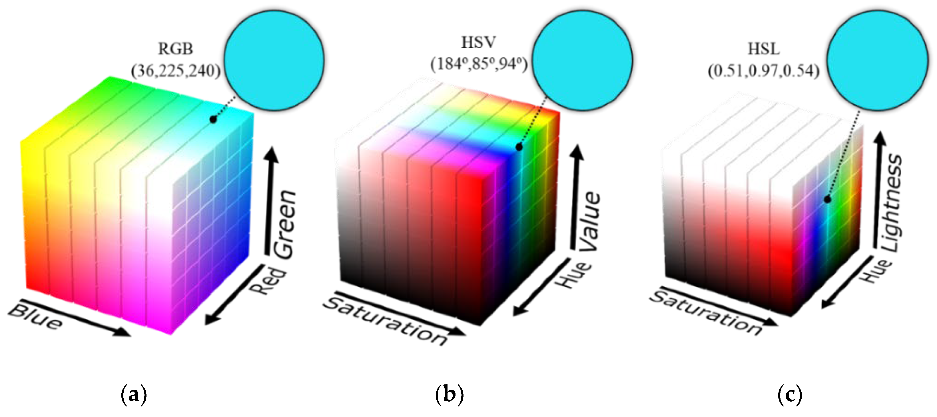
• Experiments 1. Performance comparison of models in various color spaces
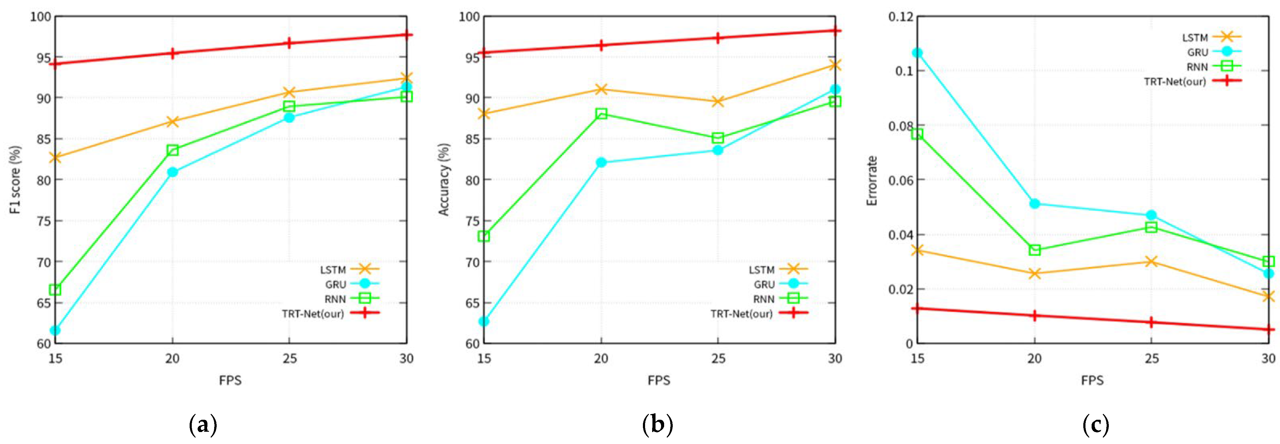
• Experiments 2. Performance comparison of models according to the fps
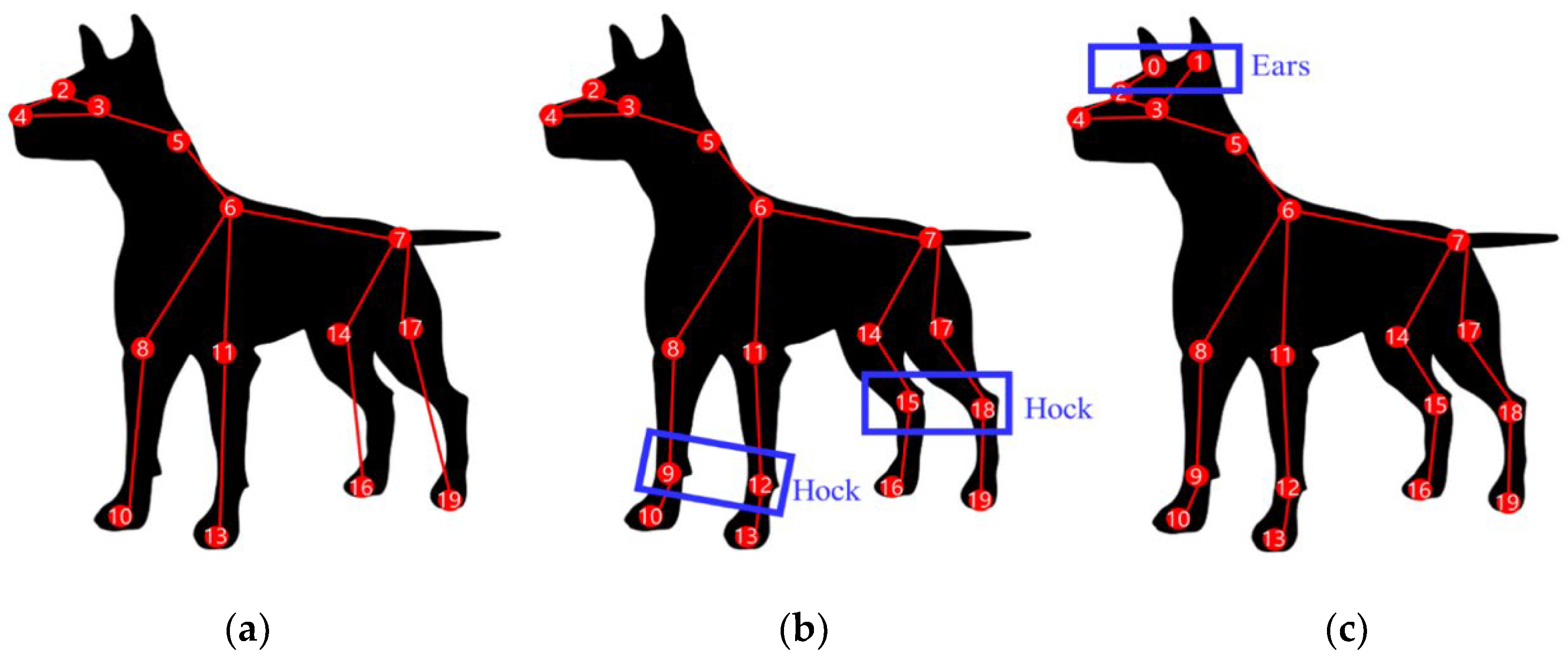
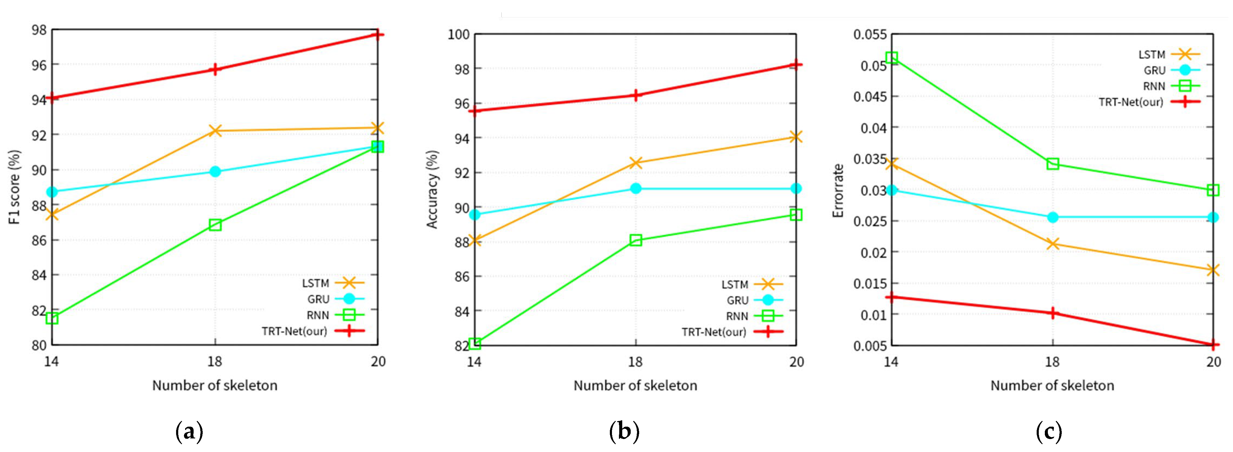
• Experiments 3. Performance comparison of models according to the number of skeleton joints
• Experiments 4. Analysis of joints that the CNN model mainly learns for each behavior

The proposed method and the conventional models compared were constructed in a structure in which the best performance is output. Figure 6 shows the structures of the proposed method and the compared models. In every compared model, four layers and 100 cells were used, and the number of epochs was set to 1000. For the optimizer, Adagrad, which solves through a reduction of the learning rate, was used. The learning rate was set to 0.01, and the decay was set to 0.0.

4.3. Experiments and Results

In the performance assessment of the classification model, the performance should be measured by considering not just the ground truths, but also errors, because no perfect answer can be obtained. Therefore, the accuracy, precision, recall, f1 score, and error rate (MSE) were used as the performance metrics for the dog behavioral pose classification during every experiment. The MSE was used as the error rate because it is calculated by considering the error in the correct answer rate not only for the ground truth, but also for other incorrect answers. The assessment formulas used are shown in Equations (7)–(11). In Equations (7)–(10), TP indicates a true positive, TN is a true negative, FP indicates a false positive, and FN is a false negative. In Equation (11), $Y_i$ represents the real observation value, and $\widehat{Y_i}$ represents the predicted value.

$$Accuracy=\frac{TP+TN}{TP+FP+FN+TN}$$

(7)

$$Precision=\frac{TP}{TP+FP}$$

(8)

$$Recall=\frac{TP}{TP+FN}$$

(9)

$$F1 score=\frac{2\left(Recall\ast Precision\right)}{Recall+Precision}=\frac{2TP}{2TP+FP+FN}$$

(10)

$$MSE=\frac{1}{d{f}_E}{\displaystyle \sum }{\left(Y_i-\widehat{Y_i}\right)}^2$$

(11)

Experiments 1. Performance comparison based on color space.

To increase the behavioral pose classification performance of dogs, it is important to maintain the identity of the original data, knowing the relationships between the extracted skeletons and the relationships among the behavior sequences. Furthermore, even for the same data values, the form of the numerical data and the expressed color vary depending on which color space they are based on. Therefore, it is important to know the color space, based upon which the numerical data are represented and learned. In this study, we propose a method for representing the relationships of dog behavior data in RGB color. Herein, we conducted an analysis to identify the color space, for which the dog behavior data show the best behavioral classification performance.

Many color spaces such as RGB, YCbCr, and HSV are used in the field of image recognition. In the experiments, we compared the performance between the models in the RGB, HSV, and HSL spaces, which are the most commonly used among the many color spaces in the computer vision field. The RGB color space is based on what was described in Section 3.2.2, and the HSV and HSL color spaces are calculated based on the RGB color space.

RGB$\to$HSV Color Space Conversion. Normalized values of RGB are used, and for the method of converting from RGB into HSV, we use a method proposed by Travis et al. [32]. RGB values are converted into HSV values. HSV includes the hue, saturation-chroma, and brightness values.

RGB$\to$HSL Color Space Conversion. For the method of converting from RGB to HSL, we use a method proposed by Saravanan et al. [33]. The RGB values are converted into HSL values.

The RGB color model is a color model created mostly for use in systems or hardware, and the HSV and HSL color models are user-oriented color models based on the color perception of humans [33]. As shown in Figure 7, the form of the numerical data and the position of the color are represented differently depending on which color space is used, even if the color is the same. Because the represented brightness is different in each color space, even the same color shows a different value and form in each color space. Furthermore, as shown in

Table 5. Comparison of behavior classification performance according to color space.

Color Space	Accuracy	Precision	Recall	F1-Score	Error Rate (MSE)
HSV	84.23	91.54	85.87	85.33	0.045
HLS	81.84	90.48	83.69	83.01	0.034
RGB	96.95	97.52	96.74	96.97	0.008

, even for the same behavior data, the value and form, which are represented differently in each color space, have an impact on the image learning and classification results.

In Table 5, the experimental results prove that the proposed method achieves the best accuracy, precision, recall, and F1 score, as well as the minimum loss. TRT-Net learns the relationships between the skeletons and the relationships between frames together by connoting them as RGB colors. Therefore, it can compensate for the decrease in pose classification accuracy and shows a better classification performance than the conventional pose classification methods using multi-modal data. In other words, the conventional multi-modal methods have a problem in that the relationships between the features in the modality cannot be efficiently learned because the models simply learn only the numerical values of the data.

Experiments 2. Performance comparison between models according to fps.

We compared the performance of the models at various frame rates per second. Through the experiments, we compared the performance between LSTM, GRU, RNN, and the proposed TRT-Net model based on the assessment metrics of Equations (7)–(11) described earlier.

A video refers to a continuous set of countless images, and sequential images are gathered to compose one video. When 30 or more consecutive frames are processed per second, humans perceive them as a natural video that is not discontinuous. Because the frame rate felt by humans as being in real time is 30 fps, we conducted the experiments by increasing the rate from 15 to 30 fps in steps of 5 fps. Figure 8 shows the comparison of the accuracy, F1 score, and error rate between the models for each setting.

In the experimental results, our proposed method, TRT-Net, showed a higher accuracy and F1 score, as well as a lower error rate, than the other classification models at various frame rates per second, ranging from a low fps of 15 to a fps of 30, which by humans appears to be in real time. This proves that the algorithm can be used without a large change in accuracy in both low- and high-performance devices. Unlike other classification models, it consistently performs well without much performance change at various frame rates per second because it maintains the original data on the pre-fusion, even after fusion, while connotatively representing the relationships between the skeleton sequence data.

Experiments 3. Performance comparison between models according to the number of skeleton joints of a dog.

We know that dogs often express emotions or behavior by primarily using their body or tail. However, it can be seen that many emotions and behaviors are expressed in the face, including the dog’s eyes, nose, and ears, as well as in the tail and body. In particular, the movement of the dog’s ears shows their mood, condition, positive signal, or negative signal. In this study, therefore, we extracted the skeletons from the face and body of the dog through DeepLabCut [27] and conducted experiments to investigate how much impact the face and body of the dog have on the classification accuracy of its pose. As shown in Figure 9, the experiments were conducted by dividing the following cases: (a) when the ears and stifles of the dog, as proposed by Yao et al. [7], were not included (14 skeleton joints); (b) when the ears of the dog, as proposed by Kearny et al. [5], were not included (18 skeleton joints); and (c) when the ears and stifles of the dog, as proposed in this paper, were all included (20 skeleton joints). We conducted the experiments by increasing the number of skeleton joints to 14, 18, and 20 to select the most appropriate number for classifying the behavioral pose of the dog.

Figure 10 shows the accuracy, F1 score, and error rate according to the number of skeleton joints. In the experimental results, the compared models, including our proposed method, performed better with a higher accuracy and F1 score and a lower error rate in Figure 10c, which contained the coordinate values of the ears, in comparison to Figure 10a,b, which did not contain the ears. Based on the experimental results, we proved that our proposed number of skeleton joints (20) for adding the ears and stifles improved the performance of the models compared to the conventionally suggested number of skeleton joints (14 joints and 18 joints). Therefore, we also used the same number of skeleton joints, i.e., 20, that were applied in other experiments. Furthermore, through the experiments, we confirmed that the ear movement and stifles of the dog are important clues for identifying its behavior.

Experiments 4. Analysis of joints that the CNN model learns mainly for each dog behavior.

To add reliability to the results derived by the CNN model, we conducted these experiments to analyze the joints that the CNN model mainly learns. As mentioned in Section 2, although the models of the previous studies showed good performance, they had a problem in that they do not provide a sufficient explanation for the derived results of the model. To solve this problem, we produced statistics by extracting the joints that the CNN model learns mainly for each behavior.

Table 6. Body and face joints detected for each dog behavior.

Behaviors	Body Joints	Face Joints
Walking	front_right_wrist(9), front_left_wrist(12), back_left_paw(19)	right_eye(2), left_eye(3)
Standing Two legs	front_right_wrist(9), front_left_elbow(12)	right_ear(0), left_ear(1), left_eye(3)
Standing Four legs	front_right_elbow(8), front_right_wrist(9), front_left_elbow(11)	right_eye(2), left_eye(3)
Lying down	withers(6)	right_ear(0), left_ear(1), right_eye(2), left_eye(3)
Eating off ground	throat(5), withers(6), front_right_elbow(8), front_right_wrist(9)	left_ear(1)
Smelling	front_right_wrist(9)	right_ear(0), left_ear(1), right_eye(2), left_eye(3),
Convulsing	None	right_ear(0), left_ear(1), right_eye(2), left_eye(3), nose(4)

shows the statistics of the joints extracted from all behaviors. According to the experimental results, or Walking and Eating Off Ground, which are dynamic behaviors, many body joint movements were detected. In the relatively static behaviors, such as Standing on Two Legs, Standing on Four Legs and Smelling, the similar proportion of body and face joints were detected or in some cases, face joints were detected more than body joints. For behaviors such as Convulsing, mainly face joints were detected as in those cases, as dogs move their face left and right violently. Through this experiment, it can be seen that although there is less information than the movement of the body joints, the movement information of the face joints is also included.

5. Conclusions and Future Work

In this study, we proposed TRT-Net, a visual tensor fusion network of a skeleton, in which the features of the skeleton extracted based on the body of a dog are represented in color images, where a CNN learns and classifies the behavior of the dog through color images. Furthermore, after generating a histogram according to the joint frequency based on the prediction generated by CNN and the filter visualization, the pattern learned by CNN was analyzed based on this. The proposed method converts behavior data into color images and uses them to improve the accuracy in classifying the behavioral poses of the dog. The proposed method was compared to the LSTM, GRU, and RNN, which are often conventionally used as behavior classification networks. According to the experimental results, TRT-Net demonstrated that the accuracy improves by an average of 7.9% and that the F1-score improves by an average of 7.3% compared to the conventional behavior classification networks, showing that the proposed method, TRT-Net, is more effective for dog behavior classification. Furthermore, through a visualization for each layer of the CNN model, we found that the face of a dog has the greatest impact on the recognition of its dog behavior. Although the conventional classification models achieve a good performance in various behavior classification tasks, they do not explain which patterns were learned to derive the results. However, to better understand the model and gain reliability on the results derived by the model, it is important to provide a clear and analyzable basis for the decision of the model. Finally, in this study, we conducted behavior classification experiments limited to dogs. Nevertheless, this study can be a foundation for a behavioral analysis of quadruped walking animals and can be used in various fields, including abnormal behavior recognition, rehabilitation, training, and evaluation systems.

Future research plans include behavior pose classification of dogs based on automatic extraction and the collection of dog skeleton joints from videos. In addition, we plan to add more types and behaviors of dogs and improve the method in order to enable behavior recognition from new dog behavior video data, excluding the training and experimental data.

References

1. Boteju, W.J.M.; Herath, H.M.K.S.; Peiris, M.D.P.; Wathsala, A.K.P.E.; Samarasinghe, P.; Weerasinghe, L. Deep Learning Based Dog Behavioural Monitoring System. In Proceedings of the 2020 3rd International Conference on Intelligent Sustainable Systems (ICISS), Thoothukudi, India, 3–5 December 2020; pp. 82–87. [Google Scholar]
2. Komori, Y.; Ohno, K.; Fujieda, T.; Suzuki, T.; Tadokoro, S. Detection of continuous barking actions from search and rescue dogs’ activities data. In Proceedings of the 2015 IEEE/RSJ International Conference on Intelligent Robots and Systems (IROS), Hamburg, Germany, 28 September–2 October 2015; pp. 630–635. [Google Scholar]
3. Brugarolas, R.; Roberts, D.; Sherman, B.; Bozkurt, A. Posture estimation for a canine machine interface based training system. In Proceedings of the 2012 Annual International Conference of the IEEE Engineering in Medicine and Biology Society, San Diego, CA, USA, 28 August–1 September 2012; pp. 4489–4492. [Google Scholar]
4. Mealin, S.; Domínguez, I.X.; Roberts, D.L. Semi-supervised classification of static canine postures using the Microsoft Kinect. In Proceedings of the Third International Conference on Animal-Computer Interaction, Milton Keynes, UK, 15–17 November 2016; pp. 1–4. [Google Scholar]
5. Kearney, S.; Li, W.; Parsons, M.; Kim, K.I.; Cosker, D. RGBD-dog: Predicting canine pose from RGBD sensors. In Proceedings of the IEEE/CVF Conference on Computer Vision and Pattern Recognition, Seattle, WA, USA, 14–19 June 2020; pp. 8336–8345. [Google Scholar]
6. Bleuer-Elsner, S.; Zamansky, A.; Fux, A.; Kaplun, D.; Romanov, S.; Sinitca, A.; van der Linden, D. Computational analysis of movement patterns of dogs with ADHD-like behavior. Animals 2019, 9, 1140. [Google Scholar] [CrossRef] [PubMed] [Green Version]
7. Yao, Y.; Jafarian, Y.; Park, H.S. Monet: Multiview semi-supervised keypoint detection via epipolar divergence. In Proceedings of the IEEE/CVF International Conference on Computer Vision, Seoul, Korea, 27 October–2 November 2019; pp. 753–762. [Google Scholar]
8. Luo, J.; Wang, W.; Qi, H. Spatio-temporal feature extraction and representation for RGB-D human action recognition. Pattern Recognit. Lett. 2014, 50, 139–148. [Google Scholar] [CrossRef]
9. Arivazhagan, S.; Shebiah, R.N.; Harini, R.; Swetha, S. Human action recognition from RGB-D data using complete local binary pattern. Cognit. Syst. Res. 2019, 58, 94–104. [Google Scholar] [CrossRef]
10. Makantasis, K.; Voulodimos, A.; Doulamis, A.; Bakalos, N.; Doulamis, N. Space-Time Domain Tensor Neural Networks: An Application on Human Pose Classification. In Proceedings of the 2020 25th International Conference on Pattern Recognition (ICPR), Milan, Italy, 10–15 January 2021; pp. 4688–4695. [Google Scholar]
11. Patel, C.I.; Garg, S.; Zaveri, T.; Banerjee, A.; Patel, R. Human action recognition using fusion of features for unconstrained video sequences. Comput. Electr. Eng. 2018, 70, 284–301. [Google Scholar] [CrossRef]
12. Zhou, L.; Chen, Y.; Wang, J.; Lu, H. Progressive bi-c3d pose grammar for human pose estimation. In Proceedings of the AAAI Conference on Artificial Intelligence, New York, NY, USA, 7–12 February 2020; Volume 34, pp. 13033–13040. [Google Scholar]
13. Wang, P.; Li, Z.; Hou, Y.; Li, W. Action recognition based on joint trajectory maps using convolutional neural networks. In Proceedings of the 24th ACM International Conference on Multimedia, New York, NY, USA, 15–19 October 2016; pp. 102–106. [Google Scholar]
14. Park, S.H.; Park, Y.H. Audio-visual tensor fusion network for piano player posture classification. Appl. Sci. 2020, 10, 6857. [Google Scholar] [CrossRef]
15. Jiang, W.; Yin, Z. Human activity recognition using wearable sensors by deep convolutional neural networks. In Proceedings of the 23rd ACM International Conference on Multimedia, Shanghai, China, 23–26 June 2015; pp. 1307–1310. [Google Scholar]
16. Ke, Q.; Bennamoun, M.; An, S.; Sohel, F.; Boussaid, F. A new representation of skeleton sequences for 3d action recognition. In Proceedings of the IEEE Conference on Computer Vision and Pattern Recognition, Honolulu, HI, USA, 21–26 July 2017; pp. 3288–3297. [Google Scholar]
17. Aubry, S.; Laraba, S.; Tilmanne, J.; Dutoit, T. Action recognition based on 2D skeletons extracted from RGB videos. MATEC Web. Conf. 2019, 277, 02034. [Google Scholar] [CrossRef]
18. Zaremba, W.; Sutskever, I.; Vinyals, O. Recurrent neural network regularization. arXiv 2014, arXiv:1409.2329. [Google Scholar]
19. Hochreiter, S.; Schmidhuber, J. Long short-term memory. Neural Comput. 1997, 9, 1735–1780. [Google Scholar] [CrossRef] [PubMed]
20. Dey, R.; Salem, F.M. Gate-variants of gated recurrent unit (GRU) neural networks. In Proceedings of the 2017 IEEE 60th International Midwest Symposium on Circuits and Systems (MWSCAS), Medford, MA, USA, 6–9 August 2017; pp. 1597–1600. [Google Scholar]
21. Du, Y.; Wang, W.; Wang, L. Hierarchical recurrent neural network for skeleton based action recognition. In Proceedings of the IEEE Conference on Computer Vision and Pattern Recognition, Boston, MA, USA, 7–12 June 2015; pp. 1110–1118. [Google Scholar]
22. Lai, K.; Tu, X.; Yanushkevich, S. Dog identification using soft biometrics and neural networks. In Proceedings of the 2019 International Joint Conference on Neural Networks (IJCNN), Budapest, Hungary, 14–19 July 2019; pp. 1–8. [Google Scholar]
23. Liu, J.; Kanazawa, A.; Jacobs, D.; Belhumeur, P. Dog breed classification using part localization. In Proceedings of the European Conference on Computer Vision, Florence, Italy, 7–13 October 2012; Springer: Berlin/Heidelberg, Germany, 2012; pp. 172–185. [Google Scholar]
24. Parkhi, O.M.; Vedaldi, A.; Zisserman, A.; Jawahar, C.V. Cats and dogs. In Proceedings of the 2012 IEEE Conference on Computer Vision and Pattern Recognition, Providence, RI, USA, 16–21 June 2012; pp. 3498–3505. [Google Scholar]
25. Moreira, T.P.; Perez, M.L.; de Oliveira Werneck, R.; Valle, E. Where is my puppy? Retrieving lost dogs by facial features. Multimed. Tools Appl. 2017, 76, 15325–15340. [Google Scholar] [CrossRef]
26. Khosla, A.; Jayadevaprakash, N.; Yao, B.; Li, F. Novel dataset for fine-grained image categorization. In Proceedings of the First Workshop on Fine-Grained Visual Categorization, IEEE Conference on Computer Vision and Pattern Recognition, Colorado Springs, CO, USA, 20–25 June 2011. [Google Scholar]
27. Mathis, A.; Mamidanna, P.; Cury, K.M.; Abe, T.; Murthy, V.N.; Mathis, M.W.; Bethge, M. DeepLabCut: Markerless pose estimation of user-defined body parts with deep learning. Nat. Neurosci. 2018, 21, 1281–1289. [Google Scholar] [CrossRef] [PubMed]
28. Ladha, C.; Hammerla, N.; Hughes, E.; Olivier, P.; Ploetz, T. Dog’s life: Wearable activity recognition for dogs. In Proceedings of the 2013 ACM International Joint Conference on Pervasive and Ubiquitous Computing, Zurich, Switzerland, 8–12 September 2013; pp. 415–418. [Google Scholar]
29. Martinez, A.R.; Liseth, E. Epilepsia En Perros: Revisi De Tema. Rev. CITECSA 2016, 6, 5. [Google Scholar]
30. Du, Y.; Fu, Y.; Wang, L. Skeleton based action recognition with convolutional neural network. In Proceedings of the 2015 3rd IAPR Asian Conference on Pattern Recognition (ACPR), Kuala Lumpur, Malaysia, 3–6 November 2015; pp. 579–583. [Google Scholar]
31. Laraba, S.; Brahimi, M.; Tilmanne, J.; Dutoit, T. 3D skeleton-based action recognition by representing motion capture sequences as 2D-RGB images. Comput. Animat. Virtual Worlds 2017, 28. [Google Scholar] [CrossRef]
32. Travis, D. Effective Color Displays: Theory and Practice; Academic Press: Cambridge, MA, USA; London, UK, 1991; ISBN 0-12-697690-2. [Google Scholar]
33. Saravanan, G.; Yamuna, G.; Nandhini, S. Real time implementation of RGB to HSV/HSI/HSL and its reverse color space models. In Proceedings of the 2016 International Conference on Communication and Signal Processing (ICCSP), Melmaruvathur, India, 6–8 April 2016; pp. 462–466. [Google Scholar]
Figure 1. Three typical multi-modality fusion strategies. (a) Simple concatenation [11], (b) late fusion [12,13], (c) AV-TFN [14], (d) MTLN [16], and (e) the proposed method (TRT-Net).
Applsci 11 11050 g001
Figure 2. Overall process of TRT-Net.
Applsci 11 11050 g002
Figure 3. Some samples from the Youtube-C7B dataset. (a) Siberian Husky, (b) Retriever and (c) French Bulldog.
Applsci 11 11050 g003
Figure 4. Configuration of the companion dog parts.
Applsci 11 11050 g004
Figure 5. Histogram-based backtracking algorithm through RGB color representation: (a) Structures of CNN Networks(step3 of Figure 2), (b) 32 feature maps in each layer, (c) Generated images through a color quantization method using K-means clustering, (d) The values of the pixels corresponding to the extracted positions are mapped to the respective RGB channels and the skeleton matrix, (e) The histogram according to the joint frequency is produced based on the extracted joint names and numbers and (f) Joints that influence the model’s decision on the behavioral image are extracted.
Applsci 11 11050 g005
Figure 6. Structure of compared models: (a) LSTM, (b) GRU, (c) RNN, and (d) TRT-Net (our approach).
Applsci 11 11050 g006
Figure 7. Expressing the color location and value according to each color model. (a) RGB color model, (b) HSV color model and (c) HSL color model.
Applsci 11 11050 g007
Figure 8. Graphs showing (a) F1 score, (b) accuracy, and (c) error rate of four models (LSTM, GRU, RNN, TRT-Net (our)).
Applsci 11 11050 g008
Figure 9. (a) Yao et al. [7], 14 skeleton joints; (b) Kearny et al. [5], 18 skeleton joints; and (c) our method, 20 skeleton joints.
Applsci 11 11050 g009
Figure 10. (a) F1 score, (b) accuracy, and (c) error rate (MSE) according to the number of skeleton joints: Yao et al. [7], 14 skeleton joints; Kearny et al. [5], 18 skeleton joints; and our method, 20 skeleton joints.
Applsci 11 11050 g010