
Machine Learning Models of COVID-19 Cases in the United States: A Study of Initial Lockdown and Reopen Regimes


International Business School, Brandeis University, Waltham, MA 02453, USA
*
Author to whom correspondence should be addressed.
Appl. Sci. 2021, 11(23), 11227; https://0-doi-org.brum.beds.ac.uk/10.3390/app112311227
Submission received: 24 September 2021
/
Revised: 12 November 2021
/
Accepted: 20 November 2021
/
Published: 26 November 2021
(This article belongs to the Special Issue Fighting COVID-19: Emerging Techniques and Aid Systems for Prevention, Forecasting and Diagnosis)
Abstract
:The purpose of this paper is to model the cases of COVID-19 in the United States from 13 March 2020 to 31 May 2020. Our novel contribution is that we have obtained highly accurate models focused on two different regimes, lockdown and reopen, modeling each regime separately. The predictor variables include aggregated individual movement as well as state population density, health rank, climate temperature, and political color. We apply a variety of machine learning methods to each regime: Multiple Regression, Ridge Regression, Elastic Net Regression, Generalized Additive Model, Gradient Boosted Machine, Regression Tree, Neural Network, and Random Forest. We discover that Gradient Boosted Machines are the most accurate in both regimes. The best models achieve a variance explained of 95.2% in the lockdown regime and 99.2% in the reopen regime. We describe the influence of the predictor variables as they change from regime to regime. Notably, we identify individual person movement, as tracked by GPS data, to be an important predictor variable. We conclude that government lockdowns are an extremely important de-densification strategy. Implications and questions for future research are discussed.
1. Introduction
SARS-CoV-2 is similar to SARS-CoV-1 and MERS-CoV in that all three are members of the Betacoronavirus genus, but they are quite different in their incubation period, symptom severity, and transmissibility [1,2]. The shorter incubation period, greater symptom severity, and lower transmissibility of both SARS-CoV-1 and MERS-CoV resulted in quick containment, and thus a higher fatality rate (deaths/cases) for both viruses. The longer incubation, lesser symptom severity (mild to none), and greater transmissibility for SARS-CoV-2 have resulted in a lower fatality for SARS-CoV-2.
Like many other countries, the United States (federal, state, and local governments) has been uneven in the enforcement of lockdowns [3,4]. Massachusetts, New York State, and Washington State had different dynamics. Washington was hit earliest as SARS-CoV-2 spread from Wuhan, China, whereas New York was hit second, likely by people entering New York City from all over the world. Rhode Island had strong border restrictions imposed by its governor, who used the national guard to divert travel from neighboring states [5].
State governors have varied in their inclination to create and enforce public health policies. Unsurprisingly, variation in compliance with public health directives has occurred. Individual freedom and economic activity have been constrained in the short-term for the long-term benefit of the public, and exacerbated by the federal government when it sent mixed messages [6]. Consequently, state governors have varied widely in their declarations of lockdowns (We use the term lockdowns rather than voluntary stay-at-home or mandatory shelter-in-place order for brevity, while acknowledging that governors in different US states have implemented them with varying degrees of strictness). In early March 2020, many governors decided it was time to impose state-wide closures of schools and non-essential businesses. The decisions were made at the state level by the governors, but a rapid cascading of lockdowns spread across the country. A substantial shift in day-to-day life began for many people. Many adults and children started to work/study primarily or exclusively from home.
Epidemiologists typically make assumptions about person-to-person contact and infer R0, the spread rate of a virus, in a Susceptible-Exposed-Infective-Recovered model [7]. Other researchers have modeled the pandemic with different methods and assumptions, depending on their analytical perspective. Operations researchers and others have used mathematical models with R0 to model the spread of the coronavirus [8,9]. Sociologists and psychologists have used survey data models [10], archival data repositories [11], meta-analyses [12], or qualitative methods [13] to provide guidance for individual and collective decision-making.
In this paper, we take a different approach. We do not make assumptions about R0. Instead, we apply machine learning at the US state level of analysis, where there is significant variation in terms of public health capabilities and policies, healthcare quality, and population health. There are also geopolitical variations in terms of population density and climate, which may make people more or less inclined to venture outdoors. Finally, political proclivities vary across the country, with different attitudes toward government, in general, and health advisories in particular [3]. We look at state characteristics as well as aggregate human behavior, including movement shown by smartphone geolocation. Our target variable for all models is the number of COVID-19 cases, i.e., patients diagnosed and under some kind of treatment.
In this paper, we analyze the spread of COVID-19 cases in the United States from 13 March 2020 to 31 May 2020. We divide this period into two regimes to reflect lockdown (13 March–15 April) and reopen (16 April–31 May). We observe this division to recognize two distinct regimes of American life. To model them as one undivided timeframe would be to disregard the different day-to-day realities of physical movement and social interactions. Each regime was a different world of individual and collective behavior with different networks, perceptions of physical risk, and different trade-offs between physical safety and economic activity. In each regime, people were prevented or discouraged from a long list of specific activities and behaviors, e.g., going to gyms or bars. In each regime, some businesses were closed or curtailed to minimize person-to-person exposure. Exceptions in all states were made for businesses considered essential, such as grocery stores and hospitals. Each regime was a new environment in which different variables of the environment were relevant and influential.
We have three general expectations based on human mobility, social distancing, and control measures (school closures, public gathering bans) implemented in China [14,15,16], as well as travel restrictions, social distancing, and home quarantine implemented in Australia [17]. All of these studies tracked, modeled, or simulated changes in COVID-19 within or between different cities, states, and regions. They generally found that restrictions, e.g., travel bans or lockdowns, were more helpful earlier in the pandemic and less helpful later in the pandemic for slowing the spread of the virus. Hence, we model the pandemic in different time regimes with location and mobility as core factors:
- We expect that the factors associated with COVID-19 cases vary substantially between the two time regimes.
- We expect that state-by-state differences are a significant driver of cases.
- We expect that human mobility is a significant driver of cases.
To model the effects of human behaviors, we recognize that direct and indirect contact may increase the likelihood of the virus spreading. In addition, both linear and non-linear relationships may be in effect. Some model variables may be common to the two regimes, whereas others are likely to be different. The case numbers may change from regime to regime as new medical treatments are discovered. Machine learning methods may be highly effective at capturing these various relationships to predict our target variable, COVID-19 cases, in different models within the regimes.
We assume that GPS data is a good metric for tracking individual movement because cell/mobile phones are nearly ubiquitous, and people rarely turn off their geolocation tracking service. Geolocation information can be aggregated and de-identified from passively collected mobile phone data, and it has been used to model the temporal and spatial dynamics of epidemics and pandemics, including malaria [18], cholera [19], measles [20], dengue [21] and Ebola [22]. It is thus an unobtrusive and non-invasive way to capture individual movement, aggregating to the state level, so that individual privacy rights are respected.
During the Spring 2020 lockdowns, there was a change in the propensity of people to travel out of state. We also note that there seemed to be a difference based on the political inclination of the state. We, therefore, choose to include Political Color, a rough indicator of the state’s governor stance on lockdowns, as one of our variables of interest in predicting COVID-19 cases.
The rest of the paper is organized as follows. We first review some technical and behavioral streams of literature in the area of public health and analytics. We then describe our methods, including data sources for the variables of interest and descriptive statistics. We then describe the results of our machine learning models and discuss our interpretation of the best model. We conclude by describing the overall research contributions, as well as limitations and future directions.
Literature Review
Detecting a shift from one regime to another can be difficult [23] because a regime is, essentially, a context with a fundamentally different set of parameters. To fit a model to one regime and to persist in applying it after a shift to a new regime, instead of fitting a new model, would cause the model to start performing poorly. One reason why it is difficult to detect a regime change is that the change can be sudden/abrupt, incremental, gradual, or recurring/oscillating [24]. In our problem, however, it is simple to detect a switch in regime, because it pertains to state lockdowns. We take the midpoint of the time window in which governors declared lockdowns as the start of the lockdown regime and the midpoint of the time window in which governors lifted their lockdowns as the start of the reopen regime.
According to theories of individual decision making and the healthcare literature, key variables to model the incidence of COVID-19 cases may include individual beliefs and perceptions, but also social factors, such as observations of other individuals, and influences from larger contexts: neighborhood norms, business environment, government restrictions, etc. [25,26]. There are “top-down” forces applying constraints (business and school closures) and “lateral forces”, i.e., person to person interactions (verbal, physical), as well as social comparisons and social mirroring, e.g., seeing others wearing a mask or maintaining a physical distance of 6+ feet. Some of these influences are explicit and processed deliberately, whereas others are cultural and largely unconscious. People generally try to behave consistent with their physical and social environments, minimizing their health risks while carrying on with their daily lives.
Under the best of circumstances, we know that individuals are boundedly rational [27,28]. They are embedded in nested and overlapping contexts of information, which attempt to empower them [29]. They need to filter out most information, which is challenging in an age of unregulated social media, or else they experience information overload. In addition, many sources of information from the media and social media contain misinformation, and many people are not able to filter the signal from the noise [30]. Software bots have been shown to create and amplify misinformation [31]. In addition, people in a pandemic may be in a sustained state of emotional distress, economic duress, and general anxiety. Overall, the assumption that people are rational decision-makers is untenable during a combination of the pandemic [20,21] and “info-demic” [32], i.e., a syndemic [33].
Focusing on the individual’s immediate environment, we note the Neighborhood Health framework [34,35]. This framework includes factors that impact human health: health hazards or stressors, the built environment, housing quality, social environments (safety, social connections, local institutions, etc.), local resources (food, exercise, recreation), and the aesthetic quality of natural spaces. All of these can have large or small but cumulative impacts. This framework is a large network of social and physical factors operating at multiple levels, with feedback loops that influence health outcomes.
The Neighborhood Health framework highlights the simultaneous effects of neighborhoods on health. Neighborhoods are both physical and social environments that have resources (and constraints), and they set boundaries for physical health exposure and set norms for appropriate behavior. During a pandemic, if one leaves home, there will be visual and verbal reminders of what is considered a significant health risk, e.g., not wearing a mask. Neighborhoods are much smaller units than a geographic state, but state policies regarding public health influence local government policies as well as the behaviors of its citizens in a top-down fashion. The impact is not deterministic, however. If one does not identify with the culture or policies of one’s state, one can choose not to comply.
The Behavioral Model of Health Services Use is a health theory that focuses on contextual factors, the environments(s) in which individuals are embedded [36]. This theory emphasizes the healthcare system and its services, which influence health behaviors. It can be thought of as an outside-in or macro-level theory of human health. These factors include population demographics, social factors, health policy, healthcare financing, organizational factors, physical environment (natural or built), population health, human genetics, and human perceptions. This large network of factors, operating at multiple levels with feedback loops, impacts health outcomes. These outcomes ultimately include the individual’s perceived health, enhanced health, overall quality of life, and satisfaction with the healthcare system.
In sum, health decisions that fail to prevent coronavirus from spreading, which may cause COVID-19, operate at many contextual levels. The individual decides whether to socialize or maintain social distance, wear a mask, and wash hands thoroughly. The individual, however, is embedded in neighborhoods within geographic states. The influence of public health recommendations from the nested governments will influence the individual directly and indirectly. The influence of trusted individuals in the individual’s peer and community network will also vary. The coronavirus will spread however it can, even as it is constrained and blocked by the decisions made at different levels. In this paper, we define and capture variables at the state level to model the incidence of COVID-19 cases.
2. Methods
Because the health or illness of individuals is impacted by the multiple levels of environments in which they live, we select a variety of variables reflecting multiple categories. Our data sources are all publicly available—none proprietary—for the sake of scientific reproducibility. Our data sources span a wide variety of providers on the principle that triangulating different sources minimizes any particular biases, assumptions, or blind spots of a particular source. It also yields a rare combination of informational signals and may thereby yield a uniquely high accuracy model. Our sources were The New York Times, The COVID Tracking Project (launched by The Atlantic), SafeGraph, America’s Health Rankings, and The Cook Political Report. For simple, objective data, e.g., population density, we used Wikipedia.
Table 1 lists all our main variables and their operationalizations, along with the data source. We develop a separate model from these variables for each of the two regimes [3]. The sample size (n) is 3996 observations, inclusive of both regimes; Lockdown Regime = 1696, Reopen Regime = 2300.
Health Rank measures the overall health of the state population and the quality of healthcare within a given state. America’s Health Rankings® is built on the World Health Organization’s definition of health, a broad indicator of the population’s overall health. It reflects the value that the state’s citizens and businesses place on health. It indicates a baseline level of health and capacity for improving it, which could breed vigilance or complacency. We divide Health Rank into three levels: High (top 10 states), Average (middle 30 states), and Bottom (lowest 10 states). We expect a negative association between Health Rank Category and COVID-19 cases because a higher rank should correspond to stronger infection prevention.
Population Density is the number of people of each state per square mile. If the density is high, there is a greater chance of person-to-person infection through close physical exposure. We expect a positive association; the greater the Population Density, the greater the number of cases because of the difficulty in maintaining a safe social distance.
Climate Temperature measures the median temperature during Spring 2020. The expectation is that warmer temperatures will make it more likely that people will leave their homes. They may reason that, if they remain socially distanced outdoors, they can minimize their risk of exposure. Moreover, when the weather is warmer, they may be more inclined to shop in stores rather than online. Climate Temperature is measured at three levels: High (top 10 states), Low (bottom 10 states), and Average (middle 30 states). We expect a positive association; the High states will be associated with a higher number of cases.
We define Political Color to be a measure of each state governor’s tendency to shutdown public activities and prohibit large gatherings. Because a pandemic is both a social and economic issue, we expect the state’s Political Color to be a useful predictor: Red (conservative) vs. Blue (liberal). We consulted several sources for conservative vs. liberal state listings and also chose to include politically Purple (moderate) states: Arizona, Florida, Pennsylvania, Wisconsin, Michigan, Maine, and North Carolina [42]. Since the Blue states were infected early, we expect them to be strongly impacted by lockdown relatively quickly. Conversely, we expect Red states, which were hit later and less severely, to be slow to impose shutdowns. We expect Purple states to be caught in the middle: impacted severely, but slow to impose shutdowns, and therefore to have the most cases.
We include GPS phone tracking data to monitor the mobility of individuals in both regimes. Location Exposure Index (LEX) was obtained through the de-identified state-level aggregation of phone data. This is based on PlaceIQ data [43]. LEX is based on signals (“pings”) obtained from smartphones responding to other smartphones or applications. LEX gives the proportion of pings received from another device or application in a different venue in the most recent 14 days. The residence of a smartphone is determined empirically from finding its presence between 5 p.m. and 9 a.m. Smartphones that do not leave their residence do not get pinged. We define LEX-In-State on a given day as the proportion of phones residing in a state that leave their home but have not been pinged in any other state over the last 14 days. LEX-Out-State on a given day is the proportion of phones residing in a state that leave their home and have been pinged in a different state over the last 14 days. LEX-Out-State gives us the tendency of people who leave their own state of residence and encounter other people. We define LEX-Total to be the sum of LEX-In-State and LEX-Out-State. Non-home-dwell-time is the median time outside the home in minutes for all devices in the home during the time period. For each device, the observed minutes outside of home across the day are summed for each device. Then the median of all the devices is calculated. We expect all LEX-based variables to be positively associated with cases.
3. Machine Learning Models: Results and Interpretation
Using all the available variables, our modeling approach was always the same, regardless of the specific machine learning method. We did the following:
- (a)
- Checked the data quality, checking for outliers, imputing for missing values, and transforming variables to be more Gaussian (Normal) to comply with statistical assumptions;
- (b)
- Partitioned the dataset randomly into Train (80%) and Test (20%) subsets. Model accuracy was determined by performance on the Test subset;
- (c)
- Checked for multi-collinearity and target leakage [44].
We tried a variety of machine learning methods in R 3.6.2. The algorithms evaluated in this paper are Multiple Regression [45], Ridge Regression [45], Elastic Net Regression, Generalized Additive Model [46,47], Gradient Boosted Machine [48], Regression Tree [45], Neural Network [45], and Random Forest [48]. The methods were selected for their known strengths in minimizing Errors of Bias and/or Errors of Variance, i.e., their ability to fit data well on hold-out data, neither underfitting nor overfitting. They also represent the range of algorithms commonly used in machine learning prediction, and they were all available as R packages.
We started with Multiple Regression as a traditional baseline method for fitting a model with only linear relationships. We then used more advanced methods to attempt to capture non-linear relationships and improve accuracy even at the cost of greater complexity and diminished interpretability:
Ridge Regression: variant of linear regression to reduce multi-collinearity and overfitting by using a different estimator, the ridge estimator, which has lower variance than the Ordinary Least Squares estimator. Regularization causes all coefficients to move toward zero, possibly becoming negative. (R package MASS)
Generalized Additive Model: a nonparametric generalization of linear regression, which allows for nonlinear relationships and coefficient regularization while maintaining interpretability. Although overfitting can occur, regularization and cross-validation help to minimize it. (R package mgcv)
Regression Tree: a decision tree method, which is non-parametric to allow for non-linear relationships between the predictor variables and the numeric target; the tree structure aids interpretability through discovered rules; simple trees can be rendered and traversed visually, aiding auditability and intuitiveness. (R package rpart)
Neural Network: generalization of linear regression with hidden layer(s) of nodes between input and output nodes; depending on the number of hidden layers, nodes per layer, and the activation function used to convert inputs to outputs, an arbitrarily complex model can be fit; may result in overfitting. (R package neuralnet)
Gradient Boosted Machine: an ensemble of sequential trees to focus on errors of previous trees; able to find interaction effects; uses gradient descent search to rapidly minimize error via arbitrary, differentiable loss function; many trees help to ensure that the local minimum found is the global minimum. (R package LightGBM)
Random Forest: an ensemble technique to fit a large number of bootstrap-sampled aggregation (bagging) of trees along with a restricted random selection of variables at each tree split. It tends to perform very well but be difficult to interpret. (R package RandomForest)
We used three standard measures of predictive accuracy in addition to the variance explained (adjusted R-squared) of the training data: Root Mean Square Error (RMSE), Mean Absolute Error (MAE), and Symmetric Mean Absolute Percentage Error (SMAPE) [49,50]. For adjusted R-squared, the range is 0 for no variance explained to 1 for all variance explained. For RMSE, MAE, and SMAPE, smaller is better.
Table 3 shows the accuracy generally held when going from training to test partition, regardless of the method used, in the Lockdown Regime. The different accuracy measures are in general agreement, with Gradient Boosted Machine nearly always having the lowest error, indicated in gray. We choose Gradient Boosted Machine as the best method for the Lockdown Regime and show its lift and residual plots in Figure 2. The residuals are small for the entire range of COVID-19 cases (log).
In Figure 3, we see the nine variables ranked by relative importance, along with partial dependence plots for the top four: Non-home dwell time, LEX-Out-state, Population density, and LEX-Total. Variable importance is determined by the loss of predictive power if the values of the variable are permuted [51,52]. We focus on the top four variables by illustrating their partial dependence plots, starting with Non-Home Dwell Time.
In Figure 3, the partial dependence plot (Figure 3a) shows the average amount of time people spent outside their homes. That metric reflects states that were not under a strict lockdown order. Even with closed schools and businesses, most people could leave their homes. As can be seen from the plot, the higher the number of cases, the less time people dwelled outside their homes. This variable tracks the predicted and actual values best in the middle, slightly under-contributing on the low end and over-contributing on the high end of the variable range. As people perceived that it was safer to leave their residence, they were more likely to do so, including the crossing of state borders.
The second-ranked variable is LEX-Out-State travel, as seen in the partial dependence plot (Figure 3b). The plot has a shape similar to that of Non-Home Dwelling Time. The smaller the number of cases, the more time spent outside one’s state. The slope is slightly steeper in this plot versus the previous, with under-contribution of LEX-Out-State on the low end and over-contribution on the high end of the variable range.
The third-ranked variable is Population Density, which shows a slightly positive trend in plot (Figure 3c). The higher the Population Density, the greater the number of cases. The model tracks the actual values very closely. The contribution of Population Density increases gradually and then tapers off at the high end, suggesting a ceiling effect.
The fourth most important variable is LEX-Total, as seen in the partial dependence plot (Figure 3d). The plot shows that LEX-Total—the people traveling in-state or out-of-state—contributes steadily to the number of cases (log). The trend is similar to that of LEX-Out-State. LEX-Total makes an under-contribution at the low end and over-contribution at the higher end of the variable range.
There is a correlational relationship between travel and cases: increased travel is strongly and negatively associated with cases. Causally, the lower the number of cases, the more travel is deemed to be safe. Conversely, the greater the number of cases, the less travel is deemed to be safe. The more one travels, the more one is exposed to possible infection. In addition, higher Population Density compounds that risk. State-by-state differences may be attributable to certain states having greater population density or a lower level of infection but greater duration of spreading or an occasional superspreader event. Residents who live close to another state’s border are also at risk because people cross state borders when it is allowed and also when it is prohibited.
Table 4 shows the accuracy generally held when going from training to test partition, regardless of the method used, in the Reopen Regime. The different accuracy measures are in agreement, with Gradient Boosted Machine always having the lowest error, indicated in gray, and there is very little error. The adjusted R2 = 99.2% and RMSE = 0.063. We choose Gradient Boosted Machine as the best method for the Lockdown Regime and show its lift and residual plots in Figure 4.
The residuals are very small for the entire range of COVID-19 cases (logged), as can be seen in Figure 4.
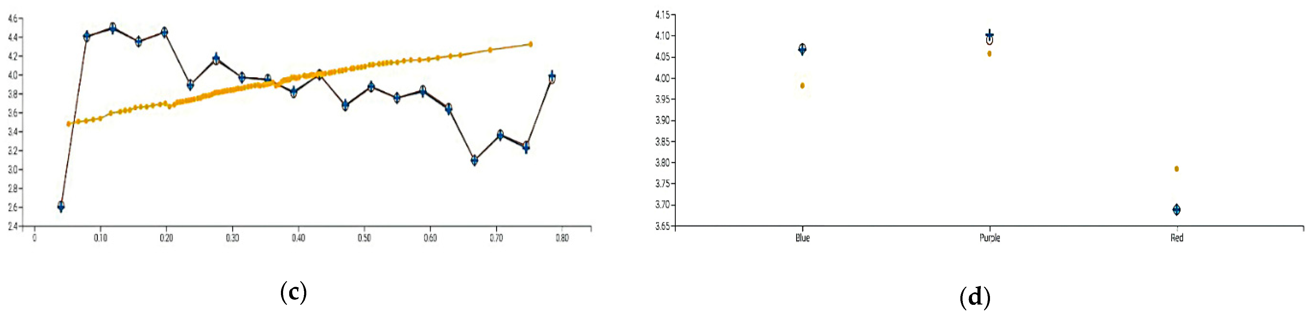
Figure 5 shows the relative importance of the variables from most to least impact: Population Density, State, LEX-Out-State, Political Color, LEX-Total, Climate Temperature, Health Rank, Non-Home Dwell Time, and Day-of-Week. We focus on the top four variables by illustrating their partial dependence plots.
In the Reopen Regime, governors were hoping that the worst of the pandemic had passed. The lockdowns were approximately one month old, and the cases were beginning to plateau. Many people had died, but more had recovered. Economic distress was growing, and businesses were looking to re-open. Jobless claims had totaled by the end of April more than 1 million each week for thirteen weeks. People needed or wanted to get back to work. Governors started to lift lockdown orders and also relax social distancing/mask mandates.
In Figure 5, the partial dependence plot (Figure 5a) shows that cases are closely tracked by population density. As population density increases, the exposure to infection from other people increases.
The second-ranked variable is State. The partial dependence plot (Figure 5b) shows State by State variation, highlighting the 19 states with the most observations and grouping the remainder under All Other. The plot shows strong predictive accuracy, even in states with fewer cases, e.g., Hawaii and Maine. The contribution of the state variable is sometimes optimal, e.g., for California and Maryland, but can be too small, e.g., Virginia, or too large, e.g., Nebraska.
The third-ranked variable is LEX-Out-State. The partial dependence plot (Figure 5c) shows that as travel out of state increases, the number of cases decreases. This is the reverse of the relationship found in the Lockdown Regime, which indicates a different temporal relationship. That is, in the Reopen Regime, the travel out of state increases because the number of cases is decreasing. In the prior, Lockdown Regime, the number of cases was increasing because out-of-state travel had increased.
The fourth-ranked variable is Political Color. The partial dependence plot (Figure 5d) shows that Red states are predicted to have lower case numbers than Blue States, and that Purple states are a bit higher than Blue States. This result is surprising, and it could indicate conflicting views of safety or information vs. misinformation or the attitude towards the lifting of lockdown and the meaning of reopening. People in Red vs. Blue states are known to have different views on the prioritization of public health vs. economic activity, in particular, and government mandates in general. Governors in Red, Blue, and Purple states reflected those views and varied significantly in their lockdown orders. Blue states, e.g., California and Massachusetts, were impacted earlier and harder than Red states but had governors who were quicker to impose lockdowns. Red states with a higher population, e.g., Texas and Arizona, were impacted later and were slower to impose lockdown orders. Some Red states with lower Population Density were impacted even later and were the slowest to impose lockdowns. The states that had the largest number of cases were the Purple states, which suggests that they were severely impacted but also had governors slow to impose lockdowns.
3.1. Discussion of Results across the Regimes
Why is GBM so effective at obtaining high accuracy, nearly almost better than the other methods, across the different regimes? In effect, the accuracy maximation problem is cast as a search task, which will efficiently find a local minimum of the loss function. By repeating the search hundreds of times and assembling the results, the local minima are likely to culminate in the global minimum, conducting a cross-validation on hold-out data guards against overfitting.
There are significant similarities and differences across the two regimes. Similarly, each regime is modeled strongly in that a GBM has low error while explaining a high proportion of the variance. Each model uses different variables, however, and their relative importance shifts significantly from regime to regime. Population Density and State, which are fixed, increase dramatically in importance, replacing Non-Home Dwell Time and LEX-Out-State, which were dynamic during the prior lockdown regime.
As shown in Table 5, the state of residence shifted from important in Lockdown Regime (relative importance = 0.349) to highly important in Reopen Regime (relative importance = 0.632). This emphasizes that states, geographically fixed themselves and with regard to neighboring states, were an essential pathway for infection. Geography matters much more than Climate Temperature or Political Color. That is, residents in a state that borders a state having a high case count will be more likely to be infected than residents of a state not bordering such a state.
In the early stage of a pandemic, human activity can and does change substantially with different government policies. Even though the policies were not strictly enforced, they were strongly suggested and followed by many people. If a lockdown was issued by a particular state’s government, people generally believed it was less safe to travel away from home, and, therefore, they exposed themselves to fewer people, thus reducing the rate of virus spread. If people are no longer under lockdown, they perceive that it is much safer to travel, even if it means encountering people who are infected.
The LEX phone tracking data does confirm that lockdowns were effective. In the reopen regime, however, it is no longer government policy or movement that has a large effect. The impacts are in effect from the prior regime, but the State of residence and the Population Density become the most important and predictive, conditional on the prior regime.
Governors varied greatly in their willingness to lockdown residents, schools, and non-essential businesses. Political Color is an important variable across both regimes, as is Health Rank. Both of these variables are amenable to long-term collective influence through changes in elected officials and healthcare systems. Health Rank is a measure of the overall health of the state’s population. This variable was found in models across both regimes, though it had small effects. States in the top level of Health Rank developed a high number of cases in both regimes. Those early lockdowns were, it seems, not imposed quickly enough nor implemented stringently enough. High Health Rank may have generated a complacency effect, in that people know that their healthcare system is high quality indulge in higher-risk behaviors, e.g., traveling out of state unnecessarily.
Toward the bottom of the list, we see Day-of-Week and Climate Temperature. Day-of-Week cannot be changed, but the availability of testing during weekends could be increased. Climate Temperature cannot be changed easily, but it can be understood better. Warmer temperatures do not stop the virus, as many hoped, but may instead tempt people to leave their homes prematurely.
3.2. Discussion of Research Contributions
Our novel contributions in this paper include (1) integrating multiple data sources, (2) dividing time into multiple regimes, and (3) highly accurate models. This research highlights the benefits of recognizing distinct regimes in order to obtain high predictive accuracy. A regime is a fundamental “sea change”, which can be difficult to recognize while it is happening. The announcement of a state-wide lockdown, however, is a clear sign that current models need to be set aside and new models developed. Moreover, it may not be necessary to capture the exact moment of transition. We tried several models at slightly different date boundaries between the regimes; it did not make a material difference. The two regimes highlight the importance of implementing strict lockdown policies to discourage movement outside the home and across state lines, which has implications from one regime to the next.
Our models were Gradient Boosted Machines in both regimes, having 95.2% and 99.2% variance explained in the lockdown and reopen regimes, respectively. The models are independent in that the model for the reopen regime did not rely on information from the lockdown regime in the form of time-lagged variables. Although the importance of the variables shifts substantially from regime to regime, they are modeled with extremely high accuracy. This suggests that although human population behavior does change, the Gradient Boosted Machine algorithm if given high quality relevant data, can adapt. These models constitute a novel and substantial contribution to the COVID-19 literature. These models are well-known machine learning methods [53,54], and the results show the power of Gradient Boosted Machines models, a particular type of ensemble model [53,54,55]. They reduce errors by combining uncorrelated submodels. In so doing, they produce a consensus from them, which tends to outperform any single model. This is the “wisdom of the crowd” [56,57,58].
Ensemble models are often considered opaque, black-box models, which are difficult to interpret and understand by human analysts but highly accurate [59]. The computational complexity enables them to obtain extremely high accuracy, but practitioners may nevertheless be reluctant to use them. Practitioners want to understand the model and be able to explain, justify, and communicate it to others. They may reason that unless the black box is at least X% more accurate than a clear-box model, where X is quite large, they cannot justify it. They would rather keep it simple, even if it is far from optimal. In addition, there may be legal, auditing, or regulatory requirements concerning transparency. If the algorithm is audited and it cannot be explained, there may be serious legal or financial consequences [60]. In order to peer inside the black-box, rendering it a grey-box so that we can understand it better, we used variable importance plots and partial dependency plots [55,60]. By having grey-box explanations we need not blindly trust the ensemble models, because we have maintained a human-in-the-loop to determine their face validity [61,62].
Another contribution of this paper is the analysis of a variety of public datasets and the vital importance of GPS data, easily obtained from de-identified data sources, to track the movement of individuals. Such tracking enables the examination of how well populations are following lockdown orders. It also enables the tracking of individuals who may be infected and the notification of nearby individuals. Google and Apple have created such a real-time, privacy-preserving contact tracing technology [63].
3.3. Limitations and Future Directions
This research has a few limitations. The data was sampled only from the fifty states of the United States. We excluded the District of Columbia and several US territories because complete data was not available for them. In the mobile phone (GPS) data, because the sources are reliable [37,38], we assumed adequate mobile phone service throughout the fifty states and no systemic differences among them.
Future research could use more granular data, e.g., county-level, and calculate the distance from the resident’s county center to the nearest state border. This would help test whether the distance from the resident’s county to their state’s border is significant, distinguishing smaller states from larger states in the risk to residents. Additionally, universities, prisons, nursing homes, long-term care, and food production facilities have been super-spreader sites. Infection rates of these venues, by state or by county, could refine our models.
The timeframe for this study was in the first half of 2020, with a sample size of 3996. The pandemic continued past our timeframe and is ongoing. State policies continue to be in flux. If lockdowns are re-instated, we will have a new regime, which calls for new data collection and modeling. In addition, vaccinations have begun, which signals the start of another new regime. With each new regime, we will need to collect and model the data again. Contact tracing phone applications have become available. Such apps—if widely adopted—would likely change the spread of the virus, signaling a new regime and calling for a new model.
How can governments financially support citizens and businesses through the loss of income during lockdowns so that they are not lifted prematurely? How can supply chains be organized to minimize the chances of panic-driven buying behavior in brick-and-mortar stores? Can emergency funds be used to subsidize home delivery of essential items so that people stay home? These larger contextual factors could extend and refine our models in future research.
Some people feel that the available vaccines were developed too quickly to be trusted, that insufficient testing was done before emergency authorization was given. These people have been misinformed, largely via social media and electronic word of mouth. Social media platforms need to do better at dispelling myths and misinformation, e.g., that warm weather makes SARS-CoV-2 disappear. The platforms could be regulated or self-regulated better so that misinformation does not spread, which would reduce the info-demic part of the syndemic [32]. On the information consumption side, users could learn how to absorb their information more critically, e.g., by preferring sources of greater credibility. Those who are more media literate may hesitate to follow public health guidelines at times, but they are more persuadable than those who are less media literate [64,65,66]. Future refinements to this research could capture different aspects of media literacy.
4. Conclusions
This research demonstrates the power of applying machine learning to different analytical regimes, thus producing highly accurate models. Such models give us insights and highlight decisions that we can make in the short- and long-term to slow or prevent an increase in COVID-19 cases. Most importantly, our models in both regimes show the predictive power of lockdowns. Lockdowns are never popular, but that is the primary contribution of this paper: the pivotal role of lockdowns in predicting COVID-19. Lockdowns need to be enforced or encouraged more strongly. In general, de-densification strategies would help prevent unnecessary gatherings of people in cities and other densely populated areas.
Overall, Population Density and LEX-Out-State were the most important variables relevant in both regimes. Although state Population Density can change in the long-term, it is immutable in the short-term. LEX-Out-State is the second most important variable overall, and it indicates people who travel across state lines, which is usually unnecessary during a pandemic. Some people do live in small states near state borders, e.g., Rhode Island or Delaware, but most essentials (food, water, medical care) are available in-state.
Traveling in-state or out-of-state can influence cases, depending on the regime. These travel variables are largely under individual control, which can be influenced by the social and physical neighborhood. If shopping can be done in bulk or delivered as needed, travel can be minimized. Similarly, if neighbors encourage each other to stay home and shop online, travel can be minimized. Finally, although state borders are open to traffic, state police can discourage cross-border traffic by stopping and questioning drivers with out-of-state license plates.
Our models were developed before the first vaccines were approved. The U.S. Food and Drug Administration has authorized vaccines from Pfizer-BioNTech, Moderna, and Johnson & Johnson. It may also authorize vaccines from other manufacturers as further clinical trials are conducted. Furthermore, the authorization of new vaccines is happening while new variants of the virus are spreading. We do not know how the new variants will impact our models, government propensity to enforce lockdowns, or peoples’ tendency to travel in-state or out-of-state.
This research raises questions for individuals and their families, as well as communities, to ponder. State was the fifth most important variable in terms of impact on cases. People may choose to better prioritize their issues and elect politicians accordingly, so that their neighbors and communities, as well as local and state representatives are guided by those priorities. Citizens would be better informed—as well as better served—by their healthcare system and elected officials. Government lockdowns would also be more likely to be timed and implemented better. If the next pandemic/syndemic is better anticipated, we will have a good chance of managing it better, thereby minimizing human and economic loss. We also need to discover effective ways of making people more media literate so that their minds are immunized against misinformation. We must remain vigilant against misinformation and complacency if we are to emerge from the current pandemic wiser and better prepared for the next one.
As of September 2021, the United States leads the world in total cases, with the fastest spread in places where people live or work in close proximity to one another: colleges/universities, jails/prisons, nursing homes/long-term care facilities, food production facilities, and states with misinformed populations. The pandemic is ongoing, and people are wary as the case counts fluctuate. This research highlights the effective use of ensemble models and what we should do in the next pandemic at multiple levels—government, business, community, and individual—to minimize the spread of infection.
Author Contributions
Conceptualization, A.K.; Data curation, Y.D., Z.Q. and C.Z.; Methodology, A.K., Y.D., Z.Q. and C.Z.; Supervision, A.K.; Validation, A.K.; Visualization, Y.D., Z.Q. and C.Z.; Writing—original draft, A.K.; Writing—review & editing, A.K. The authors contributed equally to this project. All authors have read and agreed to the published version of the manuscript.
Funding
This research received no external funding. The APC was funded by Brandeis University, International Business School.
Institutional Review Board Statement
Not applicable.
Informed Consent Statement
Not applicable.
Data Availability Statement
Public Dataset: https://dataverse.harvard.edu/dataset.xhtml?persistentId=doi:10.7910/DVN/TMFVWM, accessed on 11 November 2021.
Conflicts of Interest
The authors have no conflict of interest to declare.
References
- Petrosillo, N.; Viceconte, G.; Reginal, O.; Ippolito, G.; Petersen, E. COVID-19, SARS and MERS: Are they closely related? Clin. Microbiol. Infect. 2020, 26, 729–734. [Google Scholar] [CrossRef]
- Petersen, E.; Koopmans, M.; Go, U.; Hamer, D.H.; Petrosillo, N.; Castelli, F.; Storgaard, M.; al Khalili, S.; Simonsen, L. Comparing SARS-CoV-2 with SARS-CoV and influenza pandemics. Lancet Infect. Dis. 2020, 20, e238–e244. [Google Scholar] [CrossRef]
- Chen, C.W.; Lee, S.; Dong, M.C.; Taniguchi, M. What factors drive the satisfaction of citizens with governments’ responses to COVID-19? Int. J. Infect. Dis. 2021, 102, 327–331. [Google Scholar] [CrossRef] [PubMed]
- Gibney, E. Whose coronavirus strategy worked best? Scientists hunt most effective policies. Nat. Cell Biol. 2020, 581, 15–16. [Google Scholar] [CrossRef] [PubMed]
- Palmer, E. The Open Road Calls, but Authorities Say ‘Stop’. The New York Times, 7 August 2020. [Google Scholar]
- Lucey, C.; Ballhaus, R. White House Cautiously Optimistic About Trump’s Health after Day of Mixed Signals. The Wall Street Journal, 3 October 2020. [Google Scholar]
- Prem, K.; Liu, Y.; Russell, T.W.; Kucharski, A.J.; Eggo, R.M.; Davies, N.; Centre for the Mathematical Modelli Group; Jit, M.; Klepac, P. The Effect of Control Strategies that Reduce Social Mixing on Outcomes of the COVID-19 Epidemic in Wuhan, China: A modelling study. Lancet Public Health 2020, 5, e261–e270. [Google Scholar] [CrossRef] [Green Version]
- Cashore, J.M.; Duan, N.; Janmohamed, A.; Wan, J.; Zhang, Y.; Henderson, S.; Shmoys, D.; Frazier, P. COVID-19 Mathematical Modeling for Cornell’s Fall Semester; Cornell University: Ithaca, NY, USA, 2020. [Google Scholar]
- Kaplan, E.H. Containing 2019-nCoV (Wuhan) coronavirus. Health Care Manag. Sci. 2020, 23, 311–314. [Google Scholar] [CrossRef] [PubMed]
- Lai, J.; Ma, S.; Wang, Y.; Cai, Z.; Hu, J.; Wei, N.; Wu, J.; Du, H.; Chen, T.; Li, R.; et al. Factors associated with mental health outcomes among health care workers exposed to coronavirus disease 2019. JAMA Netw. Open 2020, 3, e203976. [Google Scholar] [CrossRef] [PubMed]
- Li, S.; Wang, Y.; Xue, J.; Zhao, N.; Zhu, T. The Impact of COVID-19 Epidemic Declaration on Psychological Consequences: A Study on Active Weibo Users. Int. J. Environ. Res. Public Health 2020, 17, 2032. [Google Scholar] [CrossRef] [PubMed] [Green Version]
- Rogers, J.P.; Chesney, E.; Oliver, D.; Pollak, T.A.; McGuire, P.; Fusar-Poli, P.; Zandi, M.; Lewis, G.; David, A. Psychiatric and neuropsychiatric presentations associated with severe coronavirus infections: A systematic review and meta-analysis with comparison to the COVID-19 pandemic. Lancet Psychiatry 2020, 7, 611–627. [Google Scholar] [CrossRef]
- Bavel, J.J.V.; Baicker, K.; Boggio, P.S.; Capraro, V.; Cichocka, A.; Cikara, M.; Crockett, M.J.; Crum, A.J.; Douglas, K.M.; Druckman, J.N. Using social and behavioural science to support COVID-19 pandemic response. Nat. Hum. Behav. 2020, 4, 460–471. [Google Scholar] [CrossRef]
- Du, B.; Zhao, Z.; Zhao, J.; Yu, L.; Sun, L.; Lv, W. Modelling the epidemic dynamics of COVID-19 with consideration of human mobility. Int. J. Data Sci. Anal. 2021, 12, 369–382. [Google Scholar] [CrossRef]
- Wu, J.T.; Leung, K.; Leung, G. Nowcasting and forecasting the potential domestic and international spread of the 2019-nCoV outbreak originating in Wuhan, China: A modelling study. Lancet 2020, 395, 689–697. [Google Scholar] [CrossRef] [Green Version]
- Hernández-Orallo, E.; Armero-Martínez, A. How Human Mobility Models Can Help to Deal with COVID-19. Electronics 2020, 10, 33. [Google Scholar] [CrossRef]
- Chang, S.L.; Harding, N.; Zachreson, C.; Cliff, O.M.; Prokopenko, M. Modelling transmission and control of the COVID-19 pandemic in Australia. Nat. Commun. 2020, 11, 5710. [Google Scholar] [CrossRef] [PubMed]
- Wesolowski, A.; Eagle, N.; Tatem, A.J.; Smith, D.L.; Noor, A.M.; Snow, R.W.; Buckee, C.O. Quantifying the Impact of Human Mobility on Malaria. Science 2012, 338, 267–270. [Google Scholar] [CrossRef] [PubMed] [Green Version]
- Peak, C.M.; Reilly, A.L.; Azman, A.S.; Buckee, C.O. Prolonging herd immunity to cholera via vaccination: Accounting for human mobility and waning vaccine effects. PLoS Negl. Trop. Dis. 2018, 12, e0006257. [Google Scholar] [CrossRef] [PubMed] [Green Version]
- Wesolowski, A.; Winter, A.; Tatem, A.J.; Qureshi, T.; Engø-Monsen, K.; Buckee, C.O.; Cummings, D.A.T.; Metcalf, C.J.E. Measles outbreak risk in Pakistan: Exploring the potential of combining vaccination coverage and incidence data with novel data-streams to strengthen control. Epidemiol. Infect. 2018, 146, 1575–1583. [Google Scholar] [CrossRef] [Green Version]
- Wesolowski, A.; Qureshi, T.; Boni, M.F.; Sundsøy, P.R.; Johansson, M.A.; Rasheed, S.B.; Engø-Monsen, K.; Buckee, C.O. Impact of human mobility on the emergence of dengue epidemics in Pakistan. Proc. Natl. Acad. Sci. USA 2015, 112, 11887–11892. [Google Scholar] [CrossRef] [Green Version]
- Peak, C.M.; Wesolowski, A.; Zu Erbach-Schoenberg, E.; Tatem, A.J.; Wetter, E.; Lu, X.; Power, D.; Weidman-Grunewald, E.; Ramos, S.; Moritz, S.; et al. Population mobility reductions associated with travel restrictions during the Ebola epidemic in Sierra Leone: Use of mobile phone data. Int. J. Epidemiol. 2018, 47, 1562–1570. [Google Scholar] [CrossRef]
- Nascimento, N.; Alencar, P.; Lucena, C.; Cowan, D. A Context-Aware Machine Learning-based Approach. In Proceedings of the 28th Annual International Conference on Computer Science and Software Engineering, Markham, ON, Canada, 29–31 October 2018. [Google Scholar]
- Gama, J.; Zliobaite, I.; Bifet, A.; Pechenizkiy, M.; Bouchachia, A. A survey on concept drift adaptation. ACM Comput. Surv. 2014, 46, 1–37. [Google Scholar] [CrossRef]
- Bandura, A. Social Foundations of Thought and Action: A Social Cognitive Theory; Prentice-Hall: Englewood Cliffs, NJ, USA, 1986. [Google Scholar]
- Fall, E.; Izaute, M.; Chakroun-Baggioni, N. How can the health belief model and self-determination theory predict both influenza vaccination and vaccination intention? A longitudinal study among university students. Psychol. Health 2018, 33, 746–764. [Google Scholar] [CrossRef] [PubMed]
- Simon, H.A. Models of Bounded Rationality; The MIT Press: Cambridge, MA, USA, 1997; Volume 2. [Google Scholar]
- Simon, H.A. Theories of Bounded Rationality. In Decision and Organisation; McGuire, C.B., Radner, R., Eds.; Elsevier: Amsterdam, The Netherlands, 1972. [Google Scholar]
- Payton, F.C.; Pare, G.; Le Rouge, C.M.; Reddy, M. Health care IT: Process, people, patients and interdisciplinary considerations. J. Assoc. Inf. Syst. 2011, 12, i–xiii. [Google Scholar] [CrossRef]
- Silver, N. The Signal and the Noise: Why So Many Predictions Fail—but Some Don’t.; The Penguin Books: New York, NY, USA, 2015. [Google Scholar]
- Benson, T. Twitter Bots Are Spreading Massive Amounts of COVID-19 Misinformation. IEEE Spectrum, 29 July 2020. [Google Scholar]
- Schillinger, D.; Chittamuru, D.; Ramírez, A.S. From “Infodemics” to Health Promotion: A Novel Framework for the Role of Social Media in Public Health. Am. J. Public Health 2020, 110, 1393–1396. [Google Scholar] [CrossRef] [PubMed]
- Valdiserri, R.; Khalsa, J.; Dan, C.; Holmberg, S.; Zibbell, J.; Holtzman, D.; Lubran, R.; Compton, W. Confronting the Emerging Epidemic of HCV Infection Among Young Injection Drug Users. Am. J. Public Health 2014, 104, 816–821. [Google Scholar] [CrossRef] [PubMed]
- Roux, A.V.D. Investigating Neighborhood and Area Effects on Health. Am. J. Public Health 2001, 91, 1783–1789. [Google Scholar] [CrossRef]
- Roux, A.V.D.; Mair, C. Neighborhoods and health. Ann. N. Y. Acad. Sci. 2010, 1186, 125–145. [Google Scholar] [CrossRef] [Green Version]
- Andersen, R.M. Revisiting the Behavioral Model and Access to Medical Care: Does it Matter? J. Health Soc. Behav. 1995, 36, 1–10. [Google Scholar] [CrossRef] [PubMed]
- New York Times. Data from The New York Times, Based on Reports from State and Local Health Agencies; New York Times: New York, NY, USA, 2020. [Google Scholar]
- The COVID Tracking Project. 2020. Available online: https://covidtracking.com/ (accessed on 23 November 2021).
- Safegraph. Social Distancing Metrics. 2020. Available online: https://docs.safegraph.com/docs/social-distancing-metrics (accessed on 23 November 2021).
- America’s Health Rankings. 2019. Available online: https://www.americashealthrankings.org/ (accessed on 23 November 2021).
- Wikipedia. List of states and territories of the United States by Population Density. 2020. Available online: https://en.wikipedia.org/wiki/List_of_states_and_territories_of_the_United_States_by_population_density (accessed on 23 November 2021).
- Cook, C.E. The Cook Political Report. 2020. Available online: https://cookpolitical.com/ (accessed on 23 November 2021).
- Couture, V.; Dingel, J.I.; Green, A.; Handbury, J.; Williams, K.R. JUE Insight: Measuring movement and social contact with smartphone data: A real-time application to COVID-19. J. Urban Econ. 2021, 103328. [Google Scholar] [CrossRef]
- Kaufman, S.; Rosset, S.; Perlich, C.; Stitelman, O. Leakage in data mining: Formulation, detection, and avoidance. ACM Trans. Knowl. Discov. Data 2011, 15, 556–563. [Google Scholar]
- Nikolopoulos, K.; Punia, S.; Schäfers, A.; Tsinopoulos, C.; Vasilakis, C. Forecasting and planning during a pandemic: COVID-19 growth rates, supply chain disruptions, and governmental decisions. Eur. J. Oper. Res. 2021, 290, 99–115. [Google Scholar] [CrossRef]
- Prata, D.N.; Rodrigues, W.; Bermejo, P.H. Temperature significantly changes COVID-19 transmission in (sub)tropical cities of Brazil. Sci. Total Environ. 2020, 729, 138862. [Google Scholar] [CrossRef]
- Qi, H.; Xiao, S.; Shi, R.; Ward, M.P.; Chen, Y.; Tu, W.; Su, Q.; Wang, W.; Wang, X.; Zhang, Z. COVID-19 transmission in Mainland China is associated with temperature and humidity: A time-series analysis. Sci. Total Environ. 2020, 728, 138778. [Google Scholar] [CrossRef] [PubMed]
- Wollenstein-Betech, S.; Silva, A.A.B.; Fleck, J.L.; Cassandras, C.G.; Paschalidis, I.C. Physiological and socioeconomic characteristics predict COVID-19 mortality and resource utilization in Brazil. PLoS ONE 2020, 15, e0240346. [Google Scholar] [CrossRef] [PubMed]
- Hyndman, R.; Koehler, A.B. Another look at measures of forecast accuracy. Int. J. Forecast. 2006, 22, 679–688. [Google Scholar] [CrossRef] [Green Version]
- Willmott, C.; Matsuura, K. Advantages of the mean absolute error (MAE) over the root mean square error (RMSE) in assessing average model performance. Clim. Res. 2005, 30, 79–82. [Google Scholar] [CrossRef]
- Janitza, S.; Strobl, C.; Boulesteix, A.-L. An AUC-based permutation variable importance measure for random forests. BMC Bioinform. 2013, 14, 119. [Google Scholar] [CrossRef] [Green Version]
- Nicodemus, K.K.; Malley, J.D.; Strobl, C.; Ziegler, A. The behaviour of random forest permutation-based variable importance measures under predictor correlation. BMC Bioinform. 2010, 11, 110. [Google Scholar] [CrossRef] [PubMed] [Green Version]
- Ke, G.; Meng, Q.; Finley, T.; Wang, T.; Chen, W.; Ma, W.; Ye, Q.; Liu, T.-Y. LightGBM: A Highly Efficient Gradient Boosting Decision Tree. In Proceedings of the Neural Information Processing Systems, Long Beach, CA, USA, 4–9 December 2017. [Google Scholar]
- Friedman, J.H. Greedy function approximation: A gradient boosting machine. Ann. Stat. 2001, 29, 1189–1232. [Google Scholar] [CrossRef]
- Bolón-Canedo, V.; Alonso-Betanzos, A. Ensembles for feature selection: A review and future trends. Inf. Fusion 2019, 52, 1–12. [Google Scholar] [CrossRef]
- Cheng, J.; Bernstein, M.S. Flock: Hybrid Crowd-Machine Learning Classifiers. In Proceedings of the 18th ACM Conference on Computer Supported Cooperative Work & Social Computing, CSCW’15, Vancouver, BC, Canada, 14–18 March 2015. [Google Scholar]
- Dissanayake, I.; Nerur, S.; Singh, R.; Lee, Y. Medical Crowdsourcing: Harnessing the “Wisdom of the Crowd” to Solve Medical Mysteries. J. Assoc. Inf. Syst. 2019, 20, 1589–1610. [Google Scholar]
- Wang, Q.; Xu, W.; Zheng, H. Combining the wisdom of crowds and technical analysis for financial market prediction using deep random subspace ensembles. Neurocomputing 2018, 299, 51–61. [Google Scholar] [CrossRef]
- Kamath, S.S.; Ananthanarayana, V.S. Semantics-based Web service classification using morphological analysis and ensemble learning techniques. Int. J. Data Sci. Anal. 2016, 2, 61–74. [Google Scholar] [CrossRef]
- Adadi, A.; Berrada, M. Peeking Inside the Black-Box: A Survey on Explainable Artificial Intelligence (XAI). IEEE Access 2018, 6, 52138–52160. [Google Scholar] [CrossRef]
- Gilpin, L.H.; Bau, D.; Yuan, B.Z.; Bajwa, A.; Specter, M.; Kagal, L. Explaining Explanations: An Overview of Interpretability of Machine Learning. In Proceedings of the 2018 IEEE 5th International Conference on Data Science and Advanced Analytics (DSAA), Turin, Italy, 1–3 October 2018; pp. 80–89. [Google Scholar]
- Kottemann, J.E.; Remus, W.E. A Study of the Relationship between Decision Model Naturalness and Performance. MIS Q. 1989, 13, 171–181. [Google Scholar] [CrossRef]
- Sharon, T. Blind-sided by privacy? Digital contact tracing, the Apple/Google API and big tech’s newfound role as global health policy makers. Ethic. Inf. Technol. 2020, 1–13. [Google Scholar] [CrossRef] [PubMed]
- Dubé, E.; Gagnon, D.; MacDonald, N.E. Strategies intended to address vaccine hesitancy: Review of published reviews. Vaccine 2015, 33, 4191–4203. [Google Scholar] [CrossRef] [PubMed] [Green Version]
- Greenberg, J.; Dubé, E.; Driedger, M. Vaccine Hesitancy: In Search of the Risk Communication Comfort Zone. PLoS Curr. 2017, 9–23. [Google Scholar]
- Salmon, D.A.; Dudley, M.Z.; Glanz, J.M.; Omer, S.B. Vaccine hesitancy: Causes, consequences, and a call to action. Vaccine 2015, 33, D66–D71. [Google Scholar] [CrossRef] [PubMed]
Figure 1.
Distributions of Numeric and Categorical Variables.

Figure 2.
Lift and Residual Plots for Gradient Boosted Machine, Lockdown Regime.

Figure 3.
Gradient Boosted Machine-Plots for Lockdown Regime. Legend: ⋅ Partial Dependence | ◦ Actual Value | + Model Prediction. (a) Log(cases)~Non-Home Dwell Time. (b) Log(cases)~LEX-Out-State. (c) Log(Cases)~Log(Population Density). (d) Log(Cases)~LEX-Total.
Figure 3.
Gradient Boosted Machine-Plots for Lockdown Regime. Legend: ⋅ Partial Dependence | ◦ Actual Value | + Model Prediction. (a) Log(cases)~Non-Home Dwell Time. (b) Log(cases)~LEX-Out-State. (c) Log(Cases)~Log(Population Density). (d) Log(Cases)~LEX-Total.


Figure 4.
Lift and Residual Plots for Gradient Boosted Machine, Reopen Regime.

Figure 5.
Gradient Boosted Machine-Plots for Reopen Regime. ⋅ Partial Dependence | ◦ Actual Value | + Model Prediction. (a) Log(Cases)~Log(Population Density). (b) Log(Cases)~State. (c) Log(Cases)~LEX-Out-State. (d) Log(Cases)~Political Color.
Figure 5.
Gradient Boosted Machine-Plots for Reopen Regime. ⋅ Partial Dependence | ◦ Actual Value | + Model Prediction. (a) Log(Cases)~Log(Population Density). (b) Log(Cases)~State. (c) Log(Cases)~LEX-Out-State. (d) Log(Cases)~Political Color.


Table 1.
Variables of Interest.
| Construct | Description | Reason | Source | Source |
|---|---|---|---|---|
| Cases | Number of people diagnosed with COVID-19 undergoing treatment | Target Variable | The New York Times, The COVID Tracking Project | [37,38] |
| LEX In-State | Location of cell/mobile phone within state of residence | Tracking physical movement of population | SafeGraph | [39] |
| LEX Out-State | Location of cell/mobile phone outside state of residence | Tracking physical movement of population | SafeGraph | [39] |
| Non-home dwell-time | Average Minutes (median) spent outside one’s own home | Physical exposure to others | SafeGraph | [39] |
| Health Rank Category | Overall health of state population based on the World Health Organization definition of health. | Health of Population influences Perceived Risk of Infection to/from Others, Behavioral Choices | America’s Health Rankings | [40] |
| Climate Temperature Category | Climate Temperature based on Spring 2020 | Physical exposure from the tendency to use public spaces in high, moderate, or low temperatures | Wikipedia | [41] |
| Political Color Category | States designated as Liberal (Blue) vs. Conservative (Red) vs. Moderate (Purple) | Political Color expected to indicate state governor’s policies toward business closures and stay-at-home orders | The Cook Political Report | [42] |
| Population Density | Population divided by Square Miles | Closer physical proximity will tend to increase the virus spread. | Wikipedia | [41] |
Table 2.
Descriptive Statistics.
| Min. | 1st Quartile | Median | Mean | 3rd Quartile | Max. | Transformation | |
|---|---|---|---|---|---|---|---|
| LEX In-State + LEX Out-State | 1.01 | 1.254 | 1.364 | 1.383 | 1.488 | 2.228 | none |
| LEX-Out-State | 0.011 | 0.266 | 0.383 | 0.402 | 0.513 | 1.289 | none |
| Non_home_dwell_time | 0 | 19 | 39 | 57.15 | 75.62 | 284 | log |
| Cases | 1 | 225 | 2318 | 14,353 | 11,712 | 375,575 | log |
| Population Density | 0.002 | 0.006 | 0.015 | 0.022 | 0.026 | 0.121 | log |
| Bottom | Average | Top | Political Color Category | ||||
| Climate Temp Category | 870 | 2738 | 968 | Blue | Purple | Red | |
| Health Rank Category | 840 | 2773 | 963 | 1827 | 677 | 2072 | |
| Days of Week | Fri | Mon | Sat | Sun | Thu | Tue | Wed |
| 664 | 631 | 670 | 676 | 652 | 637 | 646 | |
Table 3.
Accuracy Metrics for All Methods in Lockdown Regime.
| Rank | Method | Train (80%) | Test (20%) | |||||
|---|---|---|---|---|---|---|---|---|
| adj. R2 | RMSE | MAE | SMAPE | RMSE | MAE | SMAPE | ||
| 1 | Gradient Boosted Machine | 0.952 | 0.480 | 0.349 | 8.410 | 0.491 | 0.353 | 8.169 |
| 2 | Neural Network | 0.945 | 0.514 | 0.377 | 8.845 | 0.518 | 0.371 | 7.968 |
| 3 | Generalized Additive Model | 0.920 | 0.618 | 0.472 | 10.997 | 0.565 | 0.426 | 9.222 |
| 4 | Ridge Regression | 0.914 | 0.640 | 0.485 | 10.814 | 0.584 | 0.449 | 9.729 |
| 5 | Multiple Regression | 0.900 | 0.690 | 0.531 | 12.042 | 0.643 | 0.499 | 11.067 |
| 6 | Random Forest | 0.865 | 0.804 | 0.612 | 12.491 | 0.794 | 0.606 | 11.972 |
| 7 | Regression Tree | 0.835 | 0.891 | 0.626 | 13.841 | 0.923 | 0.685 | 14.452 |
Table 4.
Accuracy metrics for Reopen Regime.
| Rank | Method | Train (80%) | Test (20%) | |||||
|---|---|---|---|---|---|---|---|---|
| adj. R2 | RMSE | MAE | SMAPE | RMSE | MAE | SMAPE | ||
| 1 | Gradient Boosted Machine | 0.992 | 0.058 | 0.040 | 1.062 | 0.063 | 0.042 | 1.139 |
| 2 | Regression Tree | 0.987 | 0.075 | 0.050 | 1.305 | 0.081 | 0.053 | 1.394 |
| 3 | Ridge Regression | 0.982 | 0.090 | 0.064 | 1.669 | 0.101 | 0.069 | 1.819 |
| 4 | Generalized Additive Model | 0.983 | 0.086 | 0.063 | 1.643 | 0.100 | 0.073 | 1.907 |
| 5 | Multiple Regression | 0.979 | 0.096 | 0.068 | 1.787 | 0.109 | 0.074 | 1.980 |
| 6 | Neural Network | 0.978 | 0.098 | 0.073 | 1.913 | 0.105 | 0.078 | 2.069 |
| 7 | Random Forest | 0.974 | 0.106 | 0.079 | 2.034 | 0.113 | 0.086 | 2.243 |
Table 5.
Variable Importance Within and Across the Two Regimes for Gradient Boosted Machine.
| Lockdown Regime | Reopen Regime | Percentage Change | Average | |
|---|---|---|---|---|
| Variable | Variable Importance | Variable Importance | Variable Importance | Variable Importance |
| Pop. Density (log) | 0.546 | 1.000 | 83% | 0.773 |
| LEX-Out-State | 0.801 | 0.415 | −48% | 0.608 |
| Non-Home Dwell Time (Log) | 1.000 | 0.121 | −88% | 0.561 |
| State | 0.349 | 0.632 | 81% | 0.491 |
| LEX-Total (In-State + Out-State) | 0.530 | 0.195 | −63% | 0.363 |
| Political Color | 0.212 | 0.269 | 27% | 0.241 |
| Day-of-Week | 0.292 | 0.054 | −82% | 0.173 |
| Climate Temperature | 0.152 | 0.178 | 17% | 0.165 |
| Health Rank | 0.178 | 0.134 | −25% | 0.156 |
Publisher’s Note: MDPI stays neutral with regard to jurisdictional claims in published maps and institutional affiliations. |
© 2021 by the authors. Licensee MDPI, Basel, Switzerland. This article is an open access article distributed under the terms and conditions of the Creative Commons Attribution (CC BY) license (https://creativecommons.org/licenses/by/4.0/).
Share and Cite
MDPI and ACS Style
Kamis, A.; Ding, Y.; Qu, Z.; Zhang, C. Machine Learning Models of COVID-19 Cases in the United States: A Study of Initial Lockdown and Reopen Regimes. Appl. Sci. 2021, 11, 11227. https://0-doi-org.brum.beds.ac.uk/10.3390/app112311227
AMA Style
Kamis A, Ding Y, Qu Z, Zhang C. Machine Learning Models of COVID-19 Cases in the United States: A Study of Initial Lockdown and Reopen Regimes. Applied Sciences. 2021; 11(23):11227. https://0-doi-org.brum.beds.ac.uk/10.3390/app112311227
Chicago/Turabian StyleKamis, Arnold, Yudan Ding, Zhenzhen Qu, and Chenchen Zhang. 2021. "Machine Learning Models of COVID-19 Cases in the United States: A Study of Initial Lockdown and Reopen Regimes" Applied Sciences 11, no. 23: 11227. https://0-doi-org.brum.beds.ac.uk/10.3390/app112311227
Note that from the first issue of 2016, this journal uses article numbers instead of page numbers. See further details here.