Theoretical Framework for Determination of Linear Structures in Multidimensional Geodynamic Data Arrays

Abstract

The article addresses the issue of clustering of multidimensional data arrays with a noise using the methods of discrete mathematical analysis (DMA clustering). The theory of DMA clustering through the logical densities calculus is detailed, and the new algorithm Linear Discrete Perfect Sets (LDPS) is described. The main objective of the LDPS algorithm is to identify linearly stretched anomalies in a multidimensional array of geo-spatial data (geophysical fields, geochemistry, satellite images, local topography, maps of recent crustal movements, seismic monitoring data, etc.). These types of anomalies are associated with tectonic structures in the upper part of the Earth’s crust and pose the biggest threat for integrity of the isolation properties of the geological environment, including in regions of high-level radioactive waste disposal. The main advantage of the LDPS algorithm as compared to other cluster analysis algorithms that may be used in arrays with a noise is that it is more focused on searching for clusters that are linear. The LDPS algorithm can apply not only in the analysis of spatial natural objects and fields but also to elongated lineament structures.

1. Introduction

In 2019, the construction of an underground research laboratory (URL) was started in granitic gneiss rocks of the Nizhne–Kansky rock mass (Russia, Krasnoyarsk Territory) to justify the safety of disposal of high-level radioactive waste (HLRW). The safety of HLRW underground insulation for a period of ten thousand years or more is guaranteed due to a geological barrier. The main threat of disturbance of the isolation properties of the geological environment where HLRW are disposed is associated with large-scale geodynamic processes and phenomena.

Therefore, a priority task in the field of geo-sciences includes the analysis of multidimensional geological and geophysical data as well as the creation of a geodynamic model based on such data, which provides a forecast of the safety of the rock isolation properties over the whole period of time when the radiobiological danger of a radioactive nucleus persists [1].

In order to resolve this task, we must determine linearly stretched anomalies in a multidimensional array of geo-spatial data (geophysical fields, geochemistry, satellite images, local topography, maps of recent movements, seismic monitoring data, etc.). As is known, these types of anomalies are associated with tectonic structures in the upper part of the earth crust—faults, the boundaries of large blocks, linear structures, potential zones of possible earthquakes, etc.

These are geodynamic zones that pose the biggest threat to the isolation properties of the greatest [2]. Their search is mandatorily regulated by the statutory documents applicable in the field of HLRW disposal.

It should be emphasized that the developed methodology is very versatile and can be applied to a wide range of practical tasks of the earth sciences—in geology, geodynamics, mineral exploration, etc. Thus, this methodology is used where there is a problem in identifying linear extended anomalies from spatially referenced data of field observations. A specific link to the problem of HLRW burial in geological formations is due to the fact that these algorithms were developed in the framework of the project on this problem.

The available geospatial data arrays are almost always insufficient, uncertain and distorted due to the noise, which dictates the need for developing effective analysis and interpretation algorithms [3,4,5]. This issue is resolved in the article within the framework of discrete mathematical analysis (DMA), an original data analysis approach developed at the Geophysical Center of the Russian Academy of Sciences.

One of the development areas of discrete data analysis and discrete math is substantially related to modeling the researcher’s data analyzing skills. An experienced researcher will—better than any formal technique—distinguish any anomalies within physical fields with a small number of dimensions, move from their local level to the global one for holistic interpretation, find signals of the required form (morphology) on records of small length and many other things.

However, the researcher is helpless if faced with a large number of dimensions and volumes; therefore, a task teaching the computer in date analysis to act like a human being becomes ever more topical. When solving this task, it was considered that when the researcher thinks and operates not with numbers, but with fuzzy concepts; therefore, a technical framework for modeling includes fuzzy math and fuzzy logic along with classical math [6,7].

The advantage that researcher has in the analysis of discrete data over formal techniques is due to his or her more flexible, adaptive and stable attitude to real discrete-stochastic manifestations of fundamental mathematical properties (proximity, limitation, continuity, connectivity, trend, etc.) as compared with formal techniques, since the data analysis algorithms are built precisely on this basis as from a constructor. Hence, the plan for computer learning in the researcher’s skills is as follows: building fuzzy models for discrete counterparts of fundamental math properties and then using them according to classical math scenarios to create data analysis algorithms.

The said tasks were implemented as a researcher-oriented data analysis approach, which takes an intermediate position between hard math methods and soft combinatoric methods. This is called discrete mathematical analysis (DMA) [8,9,10,11].

This paper addresses the study of stationary data arrays representing the sets in multidimensional spaces, using the DMA methods by means of clustering. The initial concept in DMA clustering is a fuzzy model of fundamental mathematical properties, such as “limitations”. This is called density in DMA and represents a non-negative relationship between an arbitrary subset and any point in the initial finite space where the clustering is assumed to be carried out.

The value of density should be understood as a binding force between the subset and the point and interpreted as the degree of effect from the subset on the point, or, ambiguously, as the degree of limitation of the point for the subset. This view of density automatically requires that is shall be monotone over a subset: the larger the subset, the stronger its effect on the point, and it is more limiting for such subset.

Recording the density level $\alpha$ and understanding it as an ideality level, we can define any topological concept in the initial space, in particular, discrete perfection with level $\alpha$: a subset is called discrete-perfect with the level of limitation (density) $\alpha$ if it is comprised precisely of all points of the initial space $\alpha$ that are of limiting kind for such a subset.

Taking into account what was said about density above, we give an equivalent formulation of the concept of discrete-perfectness: a subset is discrete-perfect with level $\alpha$, if the strength of its connection with each of its points is not less than $\alpha$, and with any point outside the subset is strictly less than $\alpha$. Precisely this understanding of clustering formed the basis of the article and became the subject of this study. DMA has a strict theory of discrete perfect (DPS-) sets [12,13]. This serves as a methodological framework for DMA clustering and is summarized in Section 3. DMA clustering algorithms and their operation examples are shown in Section 4.

2. Review

Although there is no unified understanding of cluster, Everitt’s empirical definition of cluster is one of the largest known and most convincing definitions in cluster analysis with the following wording: “Clusters are ‘continuous’ areas of a (certain) space with a relative higher density of points, separated from other similar areas by the areas with a relatively low density of points” [14]. Subsequently, this interpretation of the cluster is referred to as empirical. It has an advantage as it does not reduce the concept of cluster to a simple form.

One possible approach to formalizing an empirical cluster is as follows: first, we introduce the idea of a dense subset against the background of the entire source space, and then a maximum subset is distinguished inside of such space, which, in turn, is broken down into connected components. The latter will be dense, isolated regions in the original space, i.e., clusters.

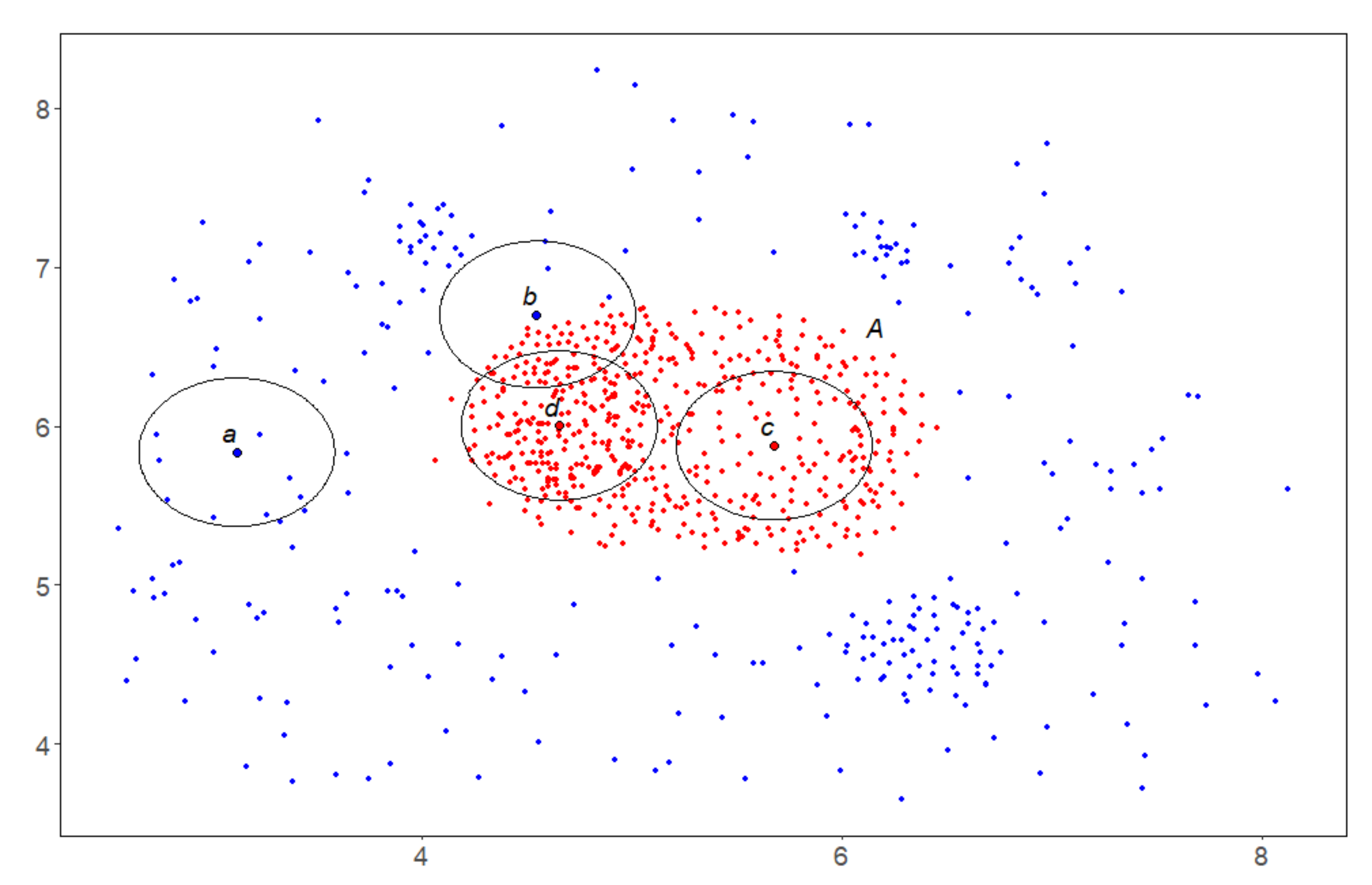
It is precisely this scenario that underlies the SDPS DMA-clustering algorithm, which came into the spotlight due to its effective applications in seismology [15]. The space where it operates is assumed to be a finite metric space (FMS), and the density of a subset at a point is equal to the number of points at its intersection with its spherical neighborhood. We will call this “sets” and designate its value by S. The concept of density relative to a set is explained in Figure 1.

With the density S and setting its level to $\alpha$, the most natural answer to the question about the density against the general background seems to be an answer in the form of a level solution, i.e., the subset of all points in the original space where the density level S is not lower than $\alpha$. However, this is only a first approximation, and it may not be sufficient: a dense point may be isolated because space is dense here and not in its neighbors. Therefore, density against the general background requires more, i.e., that each dense point has a sufficient number of dense neighbors capable of ensuring the desired level of density $\alpha$ on its own here (using its own resources).

The discrete $\alpha$-perfection of the density of “Sets” is exactly a formal expression of the above. The DMA theory of $\alpha$-perfect sets guarantees that there is such a maximum subset available within the original space and that $\alpha$-perfection will retain its property when passing to its connected components. The SDPS algorithm finds this subset and splits it into connected components. The fuzzy comparisons developed within DMA [8] allow us to effectively choose the level of limitation $\alpha$ so that the SDPS results are indeed internally indiscrete and externally dense, thus, embodying an empirical understanding of the cluster.

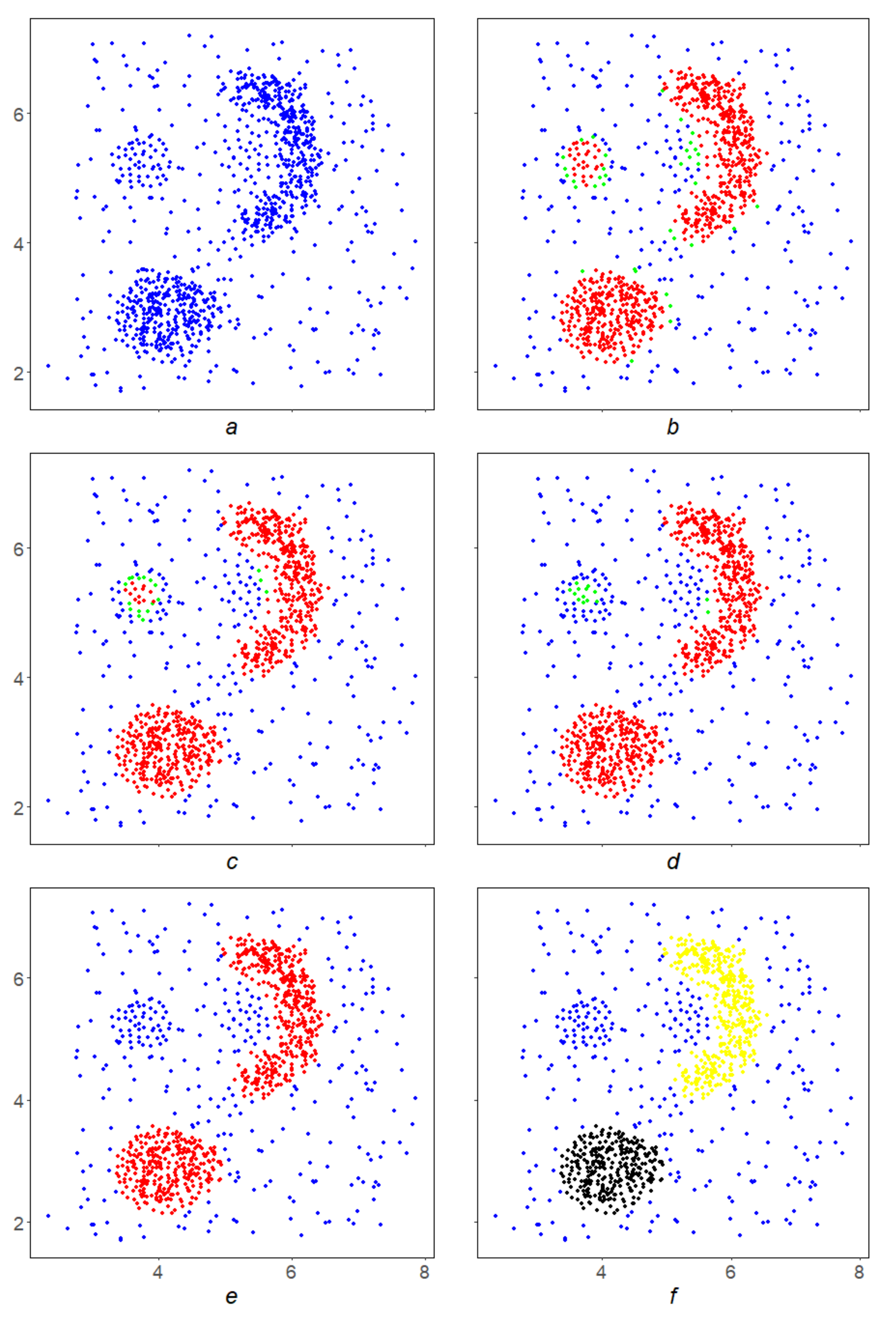
The application of the SDPS algorithm is illustrated in Figure 2. With the viewing radius for the density S and its level $\alpha$, the SDPS algorithm begins its work on the array X (Figure 2a). SDPS acts on X iteratively, sequentially in four steps (Figure 2b–e) carving out of it the desired result—a local $\alpha$-perfect subset $X(\alpha$) in X (Figure 2e). The green points in Figure 2b–d show the points that did not pass the next iteration in SDPS. SDPS further splits $X(\alpha$) into connected components (Figure 2f, yellow and black subsets).

Let us detail the SDPS algorithm within the framework of classical cluster analysis: SDPS-density algorithm of direct, free, parameter-dependent classification that does not require human involvement and does not depend on the order of space scanning [16,17]. The SDPS algorithm, like the well-known modern algorithms DBSCAN, OPTICS, and RSC [18,19,20], represents a new stage in cluster analysis, since it not only breaks the original space into homogeneous parts but also pre-clears it of noise (filters), passing to the maximum $\alpha$-perfect subset.

The use of the construction of $\alpha$-perfect sets is an essential difference of the SDPS algorithm. For example, the SDPS and DBSCAN algorithms have the same initial parameters: the radius r of the view and the density level $\alpha$ (the minimum number of points that must be in a ball of radius r). Then, they act in different ways. As mentioned above, SDPS cuts out the maximum $\alpha$-perfect set from the original space, parses it into connected components and considers them to be clusters. The DBSCAN algorithm uses an asymmetric reachability ratio, searches for regions of such reachability with centers at dense points, combines under the condition of r-proximity and considers them to be clusters.

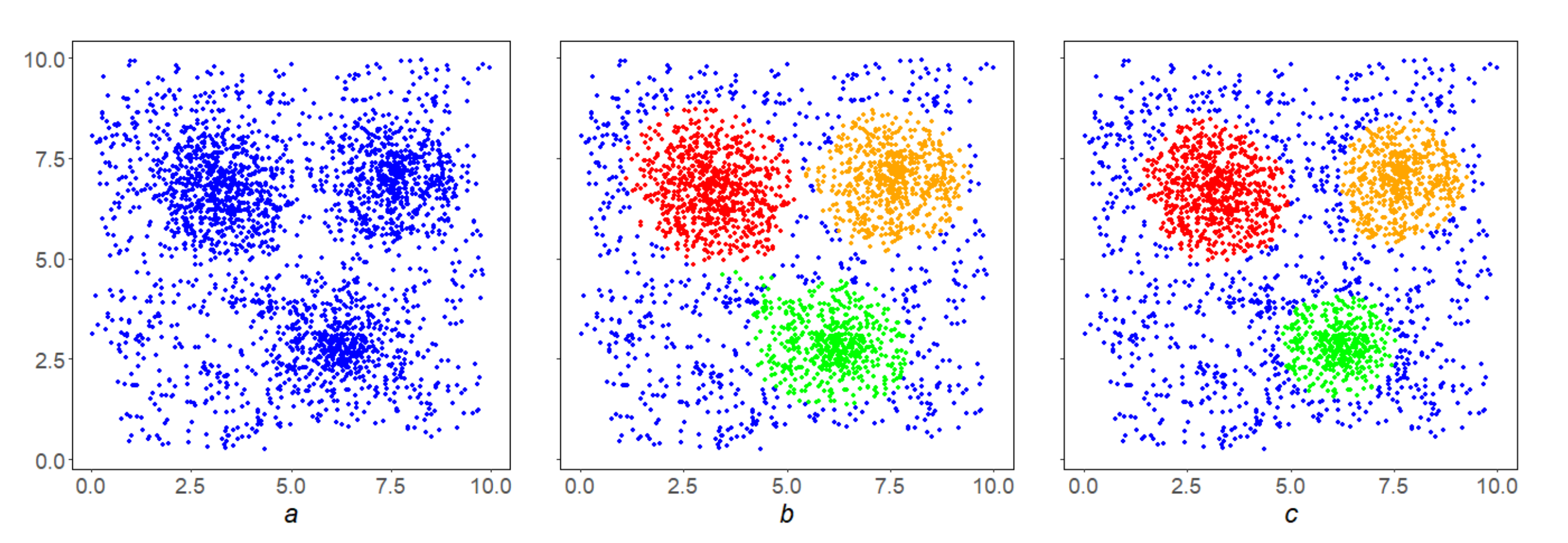
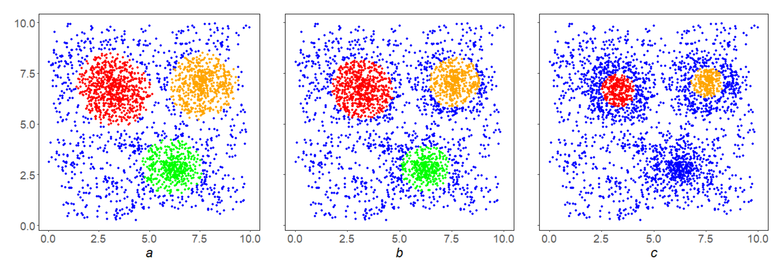
Figure 3 shows examples of clustering a complex array (Figure 3a) using algorithms: MDPS (Figure 3b), DBSCAN (Figure 3c) and OPTICS (Figure 3d). Removing noise from space and then partitioning the balance part into connected components is possible based on a large and most important class of local monotone densities. This scenario is called a DPS-scheme, and its specific implementations at a particular density are called DPS-series algorithms (DPS-algorithms). They represent the state-of-the-art DMA clustering.

Previous DMA clustering algorithms Rodin, Crystal and Monolith [21,22,23] were based on non-monotone densities, and, despite successful applications, theoretically, they had drawbacks that are characteristic of density-based cluster analysis algorithms: dependence on the order of space scanning and, as a consequence, ambiguity of results, issues with convergence, etc.

In conclusion of the general description of DMA clustering, we note that the DPS-series algorithms are extremely versatile: they are capable of working with any kind of similarity in cluster analysis (distance, correlation and associativity factors). The point is that DMA has effective procedures in place that construct monotone densities.

Let us go back to the SDPS algorithm. The resulting clusters do not have any special geometry: they are simply “continuous” and contain “much space” locally. It seems that the natural extension of research should be the search for clusters with a particular geometry. Doubtless, the first step in that process is deemed to be linear structures.

3. Materials and Methods

As mentioned in the Introduction, by clustering in the initial finite space, we mean discrete perfection with respect to the density set on it. Density is an expression in the language of fuzzy mathematics of the “limit” property. By fixing the level of the selected density in the original study, it is possible to define the reference through the normal topology. Thus, in the original dimension, there is an indexed by non-negative numbers and an ascending family of topologies. It starts at zero with the minimal inseparable topology of concatenated points and ending with the separable maximal topology of all subsets.

On an arbitrary finite metric space, one can define densities that reflect various fuzzy interpretations of the “limit” property, and some of them are used in present paper. Thus, each density on a finite metric space sets its own view of it and the corresponding research program. Density, which expresses a fuzzy interpretation of the “limit” property in a finite space, is a new concept that is not reducible to the concepts of classical mathematics, for which finite metric spaces are topologically arranged in the same way–zero-dimensional, separable.

Within the framework of this work, in the family of topologies generated on the basis of density, the property of “perfection” is of interest. We will provide a brief summary of the theory of discrete perfect sets. Its complete proof can be found in [12].

3.1. Discrete Perfect Sets

Suppose X is a finite set, and $A,B,\dots$ and $x,y,\dots$ are its subsets and points, respectively.

Definition 1.

Let us call a mapping of the product of$2^X\times X$into non-negative numbers${\mathbb{R}}^{+}$in the set X, increasing by the first argument and trivial-on-zero inputs as the density P:

$$\begin{array}{c}P(A,x)=P_A\left(x\right)\\ \forall x\in X,A\subset B\Rightarrow P_A\left(x\right)\le P_B\left(x\right),P_{⌀}\left(x\right)=0\end{array}$$

(1)

For a density P set on X and a level $\alpha \in {\mathbb{R}}^{+}$, we make a sequence of $\alpha -n-$hulls of A in X by P:

$$\begin{array}{c}{A}^1=\left\{x\in X:P_A\left(x\right)\ge \alpha \right\}\hfill \\ \dots \dots \dots \hfill \\ A^n=\left\{x\in X:P_{A\cup A^{n-1}}\left(x\right)\ge \alpha \right\}\hfill \\ \dots \dots \dots \hfill \end{array}$$

Induction on n, using the increasing monotonicity of P, establishes the following

Statment 1.

$A^1\subseteq \dots \subseteq A^n\dots$

Due to the finiteness of the set X, in the non-decreasing and bounded sequence of $\alpha -n-$hulls, starting from some number $n^{*}$, stabilization occurs:

$$A^1\subset \dots \subset A^{n^{*}}=A^{n^{*}+1}=\dots$$

(2)

Definition 2.

Let us call the set$A^{n^{*}}$$\alpha -\infty -$hull of the set A and represent it by$A^{\infty }$.

The $A^{\infty }$ set demonstrates semi-invariance: its first density hull ${\left(A^{\infty }\right)}^1$ does not fall beyond the $A^{\infty }$ set.

Statment 2.

$A^{\infty }$contains its first$\alpha$-hull by the density:

$${\left(A^{\infty }\right)}^1\subseteq A^{\infty }$$

Hence, it immediately follows that for a set $A^{\infty }$ a series (2) of its $\alpha -n-$hulls is constant.

Consequence 1.

${\left(A^{\infty }\right)}^n={\left(A^{\infty }\right)}^1\forall n\ge 2$

Let us designate $\alpha -\infty -$hull for $A^{\infty }$ through $A^{2\infty }$. Therefore:

$$A^{2\infty }={\left(A^{\infty }\right)}^{\infty }={\left(A^{\infty }\right)}^1\subseteq A^{\infty }$$

Sequentially plotting the $\alpha -\infty -$hulls based on the density P, we obtain the following scheme:

$$\begin{array}{ccccccc}A& \to & A^1& \subseteq & \dots & =& A^{\infty }\\ A^{\infty }& \supseteq & {\left(A^{\infty }\right)}^1& =& \dots & =& A^{2\infty }\\ \dots & \dots & \dots & \dots & \dots & \dots & \dots \\ A^{m\infty }& \supseteq & {\left(A^{m\infty }\right)}^1& =& \dots & =& A^{(m+1)\infty }\\ \dots & \dots & \dots & \dots & \dots & \dots & \dots \end{array}$$

Due to the X finiteness in a non-increasing sequence

$$A^{\infty }\supseteq \cdots \supseteq A^{m\infty }\supseteq \dots$$

starting with some number $m^{*}$, stabilization occurs:

$$A^{\infty }\supset \dots \supset A^{m^{*}\infty }=A^{(m^{*}+1)\infty }=\dots$$

Let us designate the set $A^{m^{*}\infty }$ by $A\left(\alpha \right)$. The process of constructing $A\left(\alpha \right)$ has a stage of increasing from $A^1$ to $A^{\infty }$ and a stage of decreasing from $A^{\infty }$ to $A\left(\alpha \right)$:

$$A\to A^1\subset \dots \subset A^{n^{*}}=A^{\infty }\supset \dots \supset A^{m^{*}\infty }=A\left(\alpha \right)$$

(3)

Statement 3.

$A\left(\alpha \right)$matches its first$\alpha$-hull.

Remark 1.

Statement 3 means that the set$A\left(\alpha \right)$is comprised exactly of those points x of space X where its density is more than α or equal to it:

$$A\left(\alpha \right)=\left\{x\in X:P_{A\left(\alpha \right)}\left(x\right)\ge \alpha \right\}.$$

Let us treat the density$P_A\left(x\right)$as a limiting measure of the point x for the set A. The point x with sufficiently large density$P_A\left(x\right)\ge \alpha$is considered to be the limiting one for A. Thus, the first hull of$A^1$represents the set of all limiting points for A in X in that sense. The points from the second hull$A^2$will, in general, be limiting points for A in X through$A^1$—that is, of the second order, etc. Statement 2 means that$A^{\infty }$is a closed set as it contains all its α-limiting points in X. Moving inside$A^{\infty }$leads to the already α-perfect set$A\left(\alpha \right)$, for restated Statement 3 means that$A\left(\alpha \right)$consists exactly of all finite points to it in X, i.e., it is a perfect one.

Definition 3.

The set A consisting of exactly all α-limiting with regard to this set points of the initial space X is called an α-discrete perfect (simply perfect, DPS-) set in X:

$$A-\mathrm{DPS}-setinX\leftrightarrow A=\{x\in X:P_A\left(x\right)\ge \alpha \}$$

Numerous studies and the examples below show that DPS-sets are condensations in X and are closely related to clustering therein. We have a way of generating them in X, i.e., $A\to A\left(\alpha \right)$ construction. It depends on four parameters: the initial space X, set A, density P and level $\alpha$:

$$A\left(\alpha \right)=A_P\left(\alpha \right|X).$$

Statement 4.

Dependencies for A, P and X are increasing dependencies, and dependence for$\alpha$are decreasing dependence:

1. 

If$A\subseteq B$, then$A\left(\alpha \right)\subseteq B\left(\alpha \right)$.

2. 

If P, Q densities on X and$P_A\left(x\right)\le Q_A\left(x\right)\forall x\in X,A\subseteq B$, then$A_P\left(\alpha \right)\le A_Q\left(\alpha \right)$.

3. 

If$\alpha <\beta$, then$A\left(\beta \right)\subseteq A\left(\alpha \right)$.

4. 

If$A\subseteq X\subset Y$and measure P are set to Y, then$A\left(\alpha \right|X)\subseteq A(\alpha \left|Y\right)$.

3.2. Complete $\mathbb{DPS}$: Scheme and Algorithms

Definition 4.

The construction process for the set A in the universe X based on the density P of its hull$A\left(\alpha \right)=A_P\left(\alpha \right|X)$is called the complete Discrete Perfect Sets algorithm and is designated through$\mathbb{DPS}$

$$\begin{array}{c}\mathbb{DPS}(·)=\mathbb{DPS}(·|X,P,\alpha ):2^X\to 2^X\\ A\to \mathbb{DPS}\left(A\right|X,P,\alpha )\to A_P\left(\alpha \right|X)=A\left(\alpha \right)\end{array}$$

Remark 2.

On a fixed space X, the$\mathbb{DPS}$algorithm depends on two parameters, the major one being the density P. In order to emphasize this fact, we will write$\mathbb{DPS}\left(P\right)$, omitting the level α, though keeping it in mind. Furthermore, we will need a broader understanding of$\mathbb{DPS}$as a correspondence$P\to \mathbb{DPS}\left(P\right)$between densities and algorithms on X. In this case, we will speak of$\mathbb{DPS}$as a scheme on X.

Generally, the DPS algorithm has two stages (3):

• increasing

  $$A^n\uparrow A^{\infty }\leftrightarrow A\subset A^1\subset \dots =A^{\infty }$$
• and decreasing

  $$A^{\infty }\downarrow A\left(\alpha \right)\leftrightarrow A^{\infty }\supset A^{2\infty }\supset \dots =A\left(\alpha \right)$$

There are situations when it works “faster” and has no more than one stage. The trivial “zero stages” case takes place for $\alpha$-perfect A.

The $\mathbb{DPS}$ algorithm constructs for each $A\subseteq X$ its perfect hull $A\left(\alpha \right)$. Given that $A\left(\alpha \right)$ is of a non-trivial kind, we consider it as a promising set in X, playing a reference role and most naturally related to A. Hull $A\left(\alpha \right)$ answers the question of the role and effect of A in X. By substituting A, through the set $\left\{A\right(\alpha );A\subseteq X\}$, we obtain the information about the structure of X at the selected level of limitation $\alpha$.

Therefore, the $\mathbb{DPS}$ algorithm is required for a thorough study of the space X through perfect hulls of its subsets, and for cluster analysis in X is too redundant and unnecessarily clumsy. Further research will show that clusters should be considered “connected pieces” of the X-maximal perfect subset $X\left(\alpha \right)$. They will be searched using a simplified version of the $\mathbb{DPS}$ algorithm DPS.

3.3. Simple DPS: Scheme and Algorithms

Throughout the entire space X, the $\mathbb{DPS}(P,\alpha )$ algorithm has only a decreasing stage, iteratively carving from X its maximum $\alpha$-perfect subset $X_P\left(\alpha \right)$, playing a major role, and therefore it has a separate name “simple Discrete Perfect Sets” algorithm and designation $\mathrm{DPS}=\mathrm{DPS}(P,\alpha )$.

The $\mathrm{DPS}(P,\alpha )$ algorithm is antagonistic by its nature to the $\mathrm{DPS}(P,\alpha )$ algorithm to a certain extent: a simple $\mathrm{DPS}(P,\alpha )$ algorithm is of global kind, intercepts the maximum perfect subset $X_P\left(\alpha \right)$ from X, whereas full $\mathrm{DPS}(P,\alpha )$ is largely of local king, passing from A to $A_P\left(\alpha \right)$ by “auto-critical crystallization”.

Remark 3.

As in Remark 2, the correspondence$P\to DPS\left(P\right)$is called a DPS scheme.$DPS\left(P\right)$algorithms are resulted from matching the densities P and a DPS scheme, and therefore they are of the same nature (DPS scheme), independent of P. There will be five such matching instances, e.g.,$SDPS=DPS\left(S\right)$, $MDPS=DPS\left(M\right)$, $FDPS=DPS\left(F\right)$, $GDPS=DPS\left(G\right)$and their complex LDPS-combination.

In this context, we are talking about them as DPS-algorithms, DPS-set algorithms.

If there is a d-metric on X space and the density P (5) is consistent with it, the $\alpha$-perfection property is inherited by “connected” components $X\left(\alpha \right)$. They are those that most accurately correspond to the idea of empirical clusters.

Subsequently, a metric d is set on X; therefore, $(X,d)$ is a FMS. For $D_A(x,r)$ we designate a full-sphere in A with the center in x radius r:

$$D_A(x,r)=\left\{a\in A:d(x,a)\le r\right\}$$

Definition 5.

Given that P is the density on X (1),$r>0$is the proximity radius. We assume that P has r-local influence (r-local) if

$$\forall x\in X.A\subseteq X\to P_A\left(x\right)=P_{D_A(x,r)}\left(x\right)$$

Based on equivalence $d(x,A)>r\leftrightarrow D_A(x,r)=⌀$ and normalization on P, it follows that

Statement 5.

If the density P is r-local, then the implication is valid

$$d(x,A)>r\to P_A\left(x\right)=0.$$

3.3.1. Topological Retreat

Two points x and y in A are called r-connected if there is a chain of r-close points in A–$x_0,\dots ,x_n$ with the starting point $x_0=x$ and terminus $x_n=y$$(d(x_i,x_{i+1})\le r,i=0,\dots ,n-1)$. The ratio of r-connectivity is an equivalence splitting the set A into components of r-connectivity $C_{r}A\left(1\right),\dots ,C_{r}A\left(k^{*}\right)$, $k^{*}=k^{*}(A,r)$:

$$A=C_{r}A\left(1\right)\vee \dots \vee C_{r}A\left(k^{*}\right).$$

(4)

Algorithmically, the split (4) is achieved as follows: let a point be in A and $C_{r}A\left(a\right)$ component of r-connectivity that contains it. Then,

$$C_{r}A\left(a\right)={\cup }_{i=1}^{\infty }{C}_r^{i}A\left(a\right)$$

where

$$\begin{array}{c}{C}_r^{0}A\left(a\right)=a\hfill \\ C_r^{1}A\left(a\right)=D_A(a,r)\hfill \\ \dots \dots \dots \dots \dots \hfill \\ C_r^{i+1}A\left(a\right)={\cup }_{\overline{a}\in C_r^{i}A\left(a\right)}{D}_A(\overline{a},r)\hfill \\ \dots \dots \dots \dots \dots \hfill \end{array}$$

By virtue of finiteness A everything is balanced and makes sense. Let us consider $C_{r}A\left(a\right)$ as the first component $C_{r}A\left(1\right)$ in (4). If it is not the last one, the same reasoning applies to $A_1=A\setminus C_{r}A\left(a\right)$. As a result, we have the second component $C_{r}A\left(2\right)$ and so on.

Statement 6.

If the density P is r-local, then every r-link component of the set$X\left(\alpha \right)$is$\alpha$-perfect.

In the event of r-local density, we will understand the $\mathrm{DPS}(P,\alpha ,r)$ algorithm through a broader lens.

Definition 6.

The process of construction for the finite metric space$(X,d)$based on the r-local density P of the α-hull$X\left(\alpha \right)$with its subsequent splitting into r-connected components is called a “simple DPS algorithm”:

$$\begin{array}{c}DPS=DPS(P,\alpha ,r)\to 2^{2^X}\hfill \\ DPS\left(X\right)=\left\{C_{r}X\left(\alpha \right)\left(1\right),\dots ,C_{r}X\left(\alpha \right)\left(k^{*}\right)\right\}\hfill \end{array}$$

Let us summarize our conversation about $\mathrm{DPS}(P,\alpha ,r)$ with its flow charts and comments to it (Figure 4).

The first stage of DPS intercepts the maximal subset $X\left(\alpha \right)$, dense against the general background, from the initial space X. The second DPS stage splits $X\left(\alpha \right)$ into components $C_{r}X\left(\alpha \right)\left(k\right)$. Each component combines density against the background and connectivity, that is, it formally expresses empirical clustering.

3.3.2. Parameter Selection: Localization Radius r

Suppose that $dX$ be the set of all non-trivial distances in X:

$$dX=\left\{d=d(x,y):x\ne y\in X\right\}$$

The localization radius r is defined as a power mean with a negative exponent d of all distances from $d\left(X\right)$:

$$r=r_q\left(X\right)={\left(\frac{{\sum }_{d\in d\left(X\right)}{d}^q}{\left|dX\right|}\right)}^{1/q}$$

(5)

3.3.3. Parameter Selection: Density Level α

The selection of level $\alpha$ greatly affects the result of the DPS algorithm. A convenient means for selecting the level $\alpha$ is fuzzy comparisons [8]. They allow us to effectively construct the limitation level so that the DPS results are really dense against the general background, that is, they are empirical clusters.

The fuzzy comparison $n(a,b)$ of two non-negative numbers a and b is a measure of the superiority of number b over number a, expressed as a scale of segment $[-1,1]$:

$$n(a,b)=mes(a<b)\in [-1,1]$$

A fuzzy comparison of a number a and a finite set B $(a\in {\mathbb{R}}^{+},B\subset {\mathbb{R}}^{+})$ can be defined as the mean of fuzzy comparisons a with all numbers from B:

$$n(a,B)=\frac{{\sum }_{b\in B}n(a,b)}{\left|B\right|},n(B,a)=\frac{{\sum }_{b\in B}n(b,a)}{\left|B\right|}$$

and understood as a measure of minimality ${mes\; min}_{B}a$ and a measure of maximality ${mes\; max}_{B}a$ of the number a against the background B:

$${mes\; min}_{B}a=n(a,B),{mes\; max}_{B}a=n(B,a).$$

The measure of maximality ${mes\; max}_{B}a$ enables formulating the necessary requirement for the DPS algorithm results: its density at each of its points must be significant (maximum enough) against the background X.

To do this, it is necessary first to calculate the density of the entire space X at all its points

$$P_X\left(X\right)=\left\{P_X\left(x\right):x\in X\right\}.$$

This is a background of X. If $\beta \in [-1,1]$ is the required level of density extremeness P against the background of X, then the immediate level $\alpha =\alpha \left(\beta \right)$ for P is uniquely determined by $\beta$ from equation

$$n(P_X\left(X\right),\alpha )=\beta ,$$

(6)

since the relation $\alpha \to n(P_X\left(X\right),\alpha )$ is of continuous and monotone kind. Equation (6) can be solved by dividing the segment at halves.

Therefore, the DPS algorithm must find a subset $X\left(\beta \right)$ in X, that is $\beta$-extremely P-dense against the general background X at each of its points:

$$x\in X\left(\beta \right)\leftrightarrow n(P_X\left(X\right),P_{X\left(\beta \right)}\left(x\right))\ge \beta \leftrightarrow P_{X\left(\beta \right)}\left(x\right)\ge \alpha \left(\beta \right)$$

and split it by the components of the r-connectivity for r from (5).

3.3.4. Quality Criterion

The DMA methods allow us to evaluate the quality $\tau (P,\alpha ,r)$ of the $\mathrm{DPS}(P,\alpha ,r)$ algorithm in a different way, as an advantage of the result $X_P(\alpha ,r)$ over complement $\overline{X_P(\alpha ,r)}$.

One of the options for the quality criterion will be discussed in Example 6.

3.4. Density

If, in comparison (6) $\alpha$ is replaced by $P_A\left(x\right)$ with arbitrary $x\in X$ and $A\subseteq X$, then we obtain a variable density alternating in sign on X with values on the scale $[-1,1]$.

Definition 7.

Density

$$mes\; max{P}_A\left(x\right)=n(P_X\left(X\right),P_A\left(x\right))$$

(7)

is called the extreme density generated by P (extreme P-density).

The value of $mes\; max{P}_A\left(x\right)$ does not clearly answer the following question: “To what extent is the subset of A dense at the point x against the general background of space X?”

It is convenient for us to consider the segment $[-1,1]$, rather than the segment $[0,1]$, as the base scale in fuzzy mathematics and fuzzy logic, and given (7), all densities are normalized to the scale $[-1,1]$. Following these assumptions, the density $P_A\left(x\right)$ at fixed A is a fuzzy structure on X. Therefore, with the help of fuzzy logic operations, as well as some others, it is possible to obtain new densities on the basis of the existing ones. This extends the capabilities of the $\mathbb{DPS}$ and DPS algorithms in space X.

Statement 7.

1. 

If P and Q are densities on X and$R=R(y_1,y_2):[-1,1]\times [-1,1]\to [-1,1]$nondecreasing mapping, then superposition

$$R{(P,Q)}_A\left(x\right)=R(P_A\left(x\right),Q_A\left(x\right))$$

will be the density on X.

2. 

If ¬ fuzzy negation on$[-1,1]$, then the superposition

$$\neg P_A\left(x\right)=\neg \left(P_{\overline{A}}\left(x\right)\right)$$

will be the density on X.

3. 

If n is a fuzzy comparison on${\mathbb{R}}^{+}$, then the superposition

$$C{(P,Q)}_A\left(x\right)=n(Q_{\overline{A}}\left(x\right),P_A\left(x\right))$$

will be the density on X.

Consequence 2.

1. 

R-connection P and$\neg P$will be the density on X

$$R{(P,\neg P)}_A\left(x\right)=R(P_A\left(x\right),\neg P_A\left(x\right))$$

2. 

If ⊤ (⊥, $M_p$) is t-norm (t-co-norm, generalized averaging operator) [7], then superpositions $\top (P_A\left(x\right),Q_A\left(x\right))$, $\perp (P_A\left(x\right),Q_A\left(x\right))$, $M_p(P_A\left(x\right),Q_A\left(x\right))$ will be densities on X.

3. 

If$\lambda \in [0,1]$, then$\lambda$-connection$\lambda P_A\left(x\right)+(1-\lambda )Q_A\left(x\right)$will be density on X.

4. 

A “fuzzy comparison”$CP$will be the density on X:

$$C{P}_A\left(x\right)=C{(P,P)}_A\left(x\right)=n(P_{\overline{A}}\left(x\right),P_A\left(x\right))$$

3.4.1. The Logical Densities Calculus

Suppose that ${\mathfrak{P}}_1,\dots ,{\mathfrak{P}}_K$ properties of elements of space X, which clusters can be obtained by the DPS algorithm with respect to densities $P_1,\dots ,P_K$.

If $\mathfrak{P}$ is a complex property obtained from properties ${\mathfrak{P}}_1,\dots ,{\mathfrak{P}}_K$ using the fuzzy logic formula Φ containing only monotone operations: $\mathfrak{P}=\mathrm{\Phi }({\mathfrak{P}}_1,\dots ,{\mathfrak{P}}_K)$ then clusters for $\mathfrak{P}$ in X can be obtained using DPS algorithm with density $P=\mathrm{\Phi }(mes\; max{P}_1,\dots ,mes\; max{P}_K)$.

Remark 4.

The schemes$\mathbb{DPS}$and DPS depend on parameters, the main of which is the density P. Connecting with it, they become algorithms$\mathbb{DPS}(P,\alpha )$and$\mathrm{DPS}(P,\alpha )$with a subordinate parameter α.

Therefore, $\mathbb{DPS}$ and DPS induce relations $P\to \mathbb{DPS}\left(P\right)$ and $P\to \mathrm{DPS}\left(P\right)$, that to a certain extent resemble “functors” from the “category of densities” to the “category of algorithms”. This enables correct understanding (“through functors”) of the results of Statement 7–Section 3.4.1: the operations described therein can be considered “functors” on densities. Their superpositions with $\mathbb{DPS}$ and DPS provide new mappings of densities into algorithms, that is, new algorithmic schemes that depend on density.

Example 1.

1. 

Scheme$\neg DPS:P\to DPS(\neg P)$

2. 

Scheme$CDPS:P\to DPS\left(CP\right)$

3. 

Scheme$(\lambda ,1-\lambda )DPS:P\to DPS(\lambda P+(1-\lambda )\neg P)$

Algorithms representing implementations of these schemes on specific densities play an important role in the FMS analysis and will be discussed below.

Remark 5.

Combination of fuzzy logic with densities gives great expressive power at the local level in studying of FMS X. On the other hand, the DPS scheme is very effective in connecting local data. These two circumstances make the DPS algorithms a powerful tool in studying of FMS X at the global scale.

The final part of the article will address the empirical evidences of this scheme by giving examples of DPS with different densities thus describing versions of DPS.

4. Results

4.1. SDPS Algorithm

Historically, the set-theoretical SDPS was the first in a series of DPS-algorithms. It is based on the density S with the name “Number of points” (“Number of space”) [12,13] and conveying the degree of concentration of space X round each of its points x (the most natural understanding of density X in x).

The density $S_A\left(x\right)$ depends on the localization radius $r=r_q\left(X\right)$ (5) and the non-negative parameter p, considering the distance to x in the full-sphere $D_A(x,r)$:

$$S_A\left(x\right)=S_A\left(x\right|q,p)=\sum _{y\in D_A(x,r)}{\left(1-\frac{d(x,y)}{r}\right)}^p$$

When $p=0$, we have the usual number of points, explaining the name S:

$$S_A\left(x\right|q,0)=\left|D_A(x,r_q)\right|$$

The S density is r-local, and the SDPS algorithm is the implementation of the DPS scheme based on S, described in Definition 6–Section 3.3.3: $\mathrm{SDPS}=\mathrm{DPS}(S,r,\beta )$. The result of SDPS is condensations in X ≡ sets locally containing “many X”. They correspond to empirical clusters in terms of the most formal criteria. By varying the SDPS parameters, it is possible to obtain a fairly complete picture of the hierarchy of clusters in X.

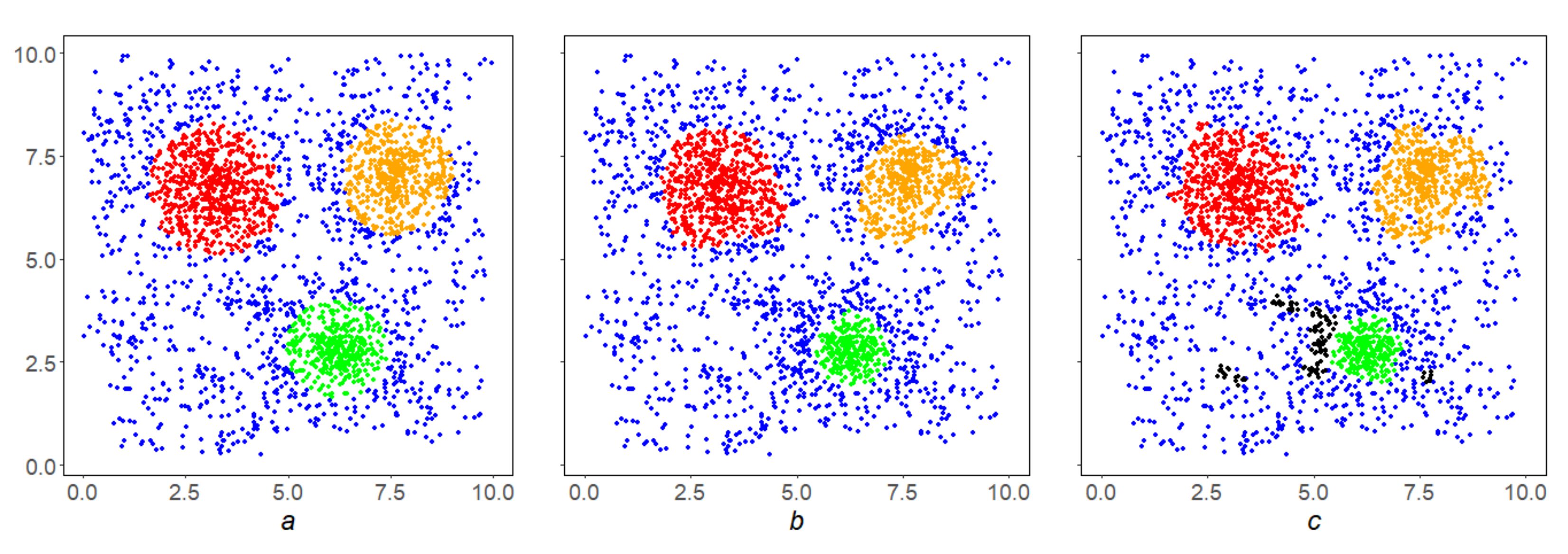
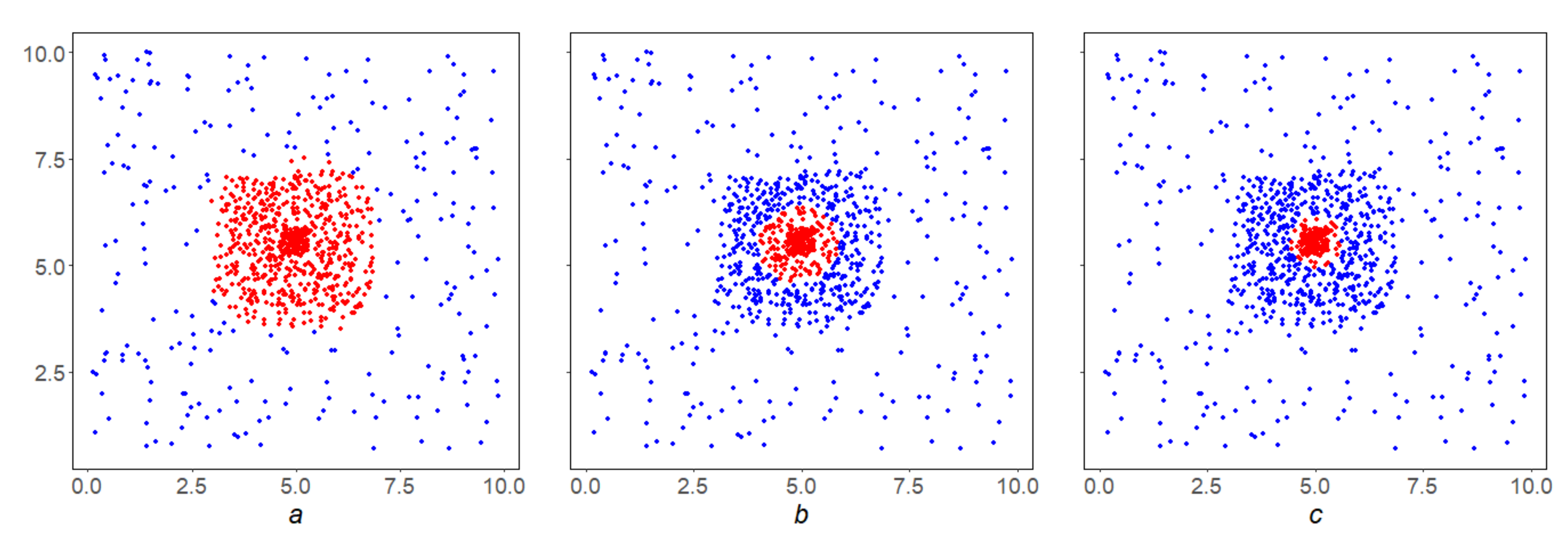
Example 2.

Figure 5b shows the result of selection by level$\beta =-0.3$for density S on the initial array X (Figure 5a), that is, the first iteration$X^1(-0.3)$of the SDPS algorithm. It contains isolated points that needs to be removed, and in this sense is inferior to the final result$X(-0.3)$of the SDPS algorithm on X (Figure 5c.)

Example 3.

In the conditions of the Example 2, the inverse correlation of the SDPS algorithm performance with the parameter β is shown. By increasing it, we go inside the condensation, finding dense nuclei inside them (Figure 6a–c).

Example 4.

In the conditions of Example 2 the direct correlation of the SDPS algorithm performance with the parameter q is shown. By lowering it, we make the SDPS algorithm more local, focusses on finding smaller condensations (Figure 7a–c). All small condensations in Figure 7c are shown in black.

Example 5.

In the conditions of the Example 2, the inverse correlation of the SDPS algorithm performance with the parameter p is shown. By increasing it, we make the SDPS algorithm more stringent (Figure 8a–c).

The above examples illustrate the general property of SDPS algorithm dependence on parameters: the stronger the localization $(p,q)$ and the density level $\beta$ is, the stricter the SDPS algorithm is, and its results are denser and finer.

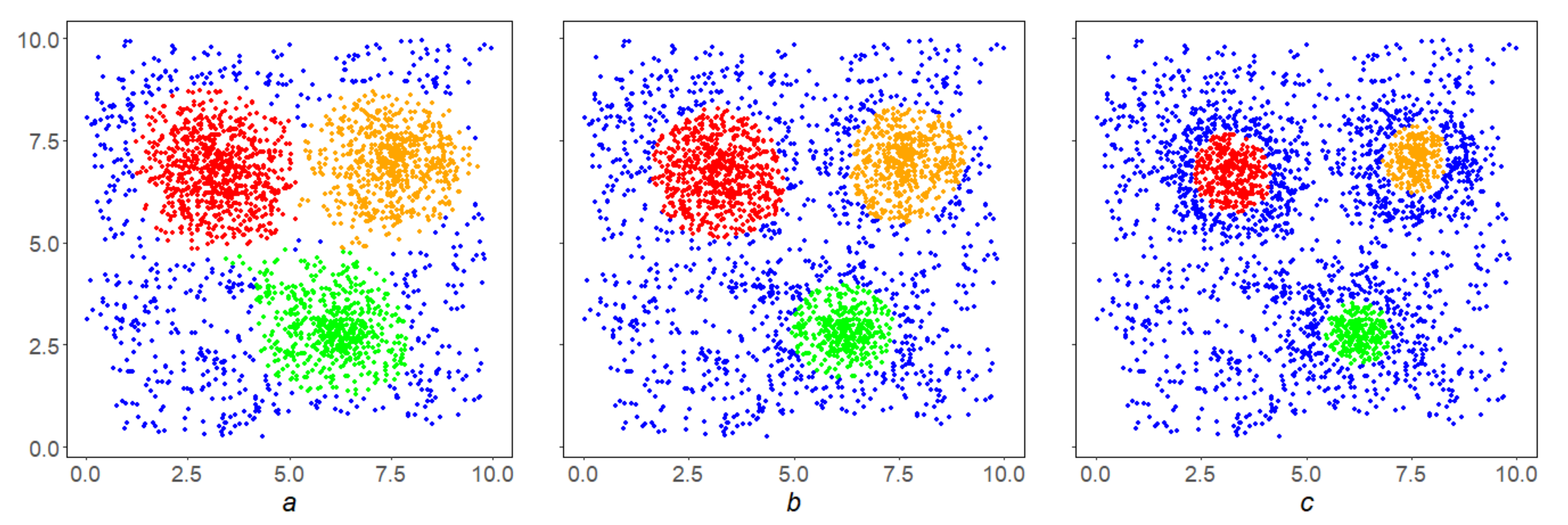
Example 6.

Let us illustrate the clustering quality$\tau (S,r,\alpha )$introduced in Section 3.3.4 on the SDPS work in the array shown in Figure 9. Let us designate by$M(\beta ,r)$and$\overline{M}(\beta ,r)$the mean densities of the sets$X_S(\beta ,r)$and$\overline{X_S(\beta ,r)}$at their points, then the result of their fuzzy comparison$\tau (\beta ,r)=n\left(\overline{M}(\beta ,r),M(\beta ,r)\right)$can be considered a version of the quality of the$SDPS(\beta ,r)$algorithm on the space X. From left to right it is equal to$0.858$, $0.595$, $0.510$respectively. This is true: the clustering in Figure 9a is clearly better, and Figure 9b,c are fairly the same.

4.2. MDPS Algorithm

The SDPS algorithm is especially effective in heterogeneous, irregular spaces, where the property “density against the background” is strongly pronounced. If it is weakly expressed, there may be disadvantages in the work of SDPS caused by the density S.

Example 7.

1. 

Suppose that X is a uniform finite grid. The nodes at the edge X have a lower density S than the central nodes, although space X looks equally homogenous in both cases.

2. 

If in a full-sphere$D_A(x,r)$all points other than x, are concentrated on the circle$C_A(x,r)$and there are many of them, then the density$S_A\left(x\right)$is significant, regardless ther-isolation x.

Another construct of the density M, which is also expressing the concentration of space X at the point x does not have such disadvantages, It is called solidity and is part of the main DMA-clustering algorithm with the correspondent name [21]. Let us talk about it.

Fix natural number $m\in \mathbb{N}$ and construct a uniform grid of nodes $r_i=\frac{ir}{m}$, $i=0,\dots ,m$ in the interval $[0,r]$. Then, we define a concentric in x semi-open ring $T_i(x,A)$ for each $i\ne 0$:

$$T_i(x,A)=\left\{y\in A:r_{i-1}<d(x,y)\le r_i\right\}$$

For each $T_i(x,A)$, we assign the relevant weight ${\psi }_i:1\ge {\psi }_1\ge \dots \ge {\psi }_m>0$. Solidity $M_A\left(x\right)$ is defined as the ratio of the sum of the weights of non-empty rings to the sum of the weights of all rings:

$$M_A\left(x\right)=\frac{{\sum }_{T_i\left(x\right)\ne 0}{\psi }_i}{{\sum }_{i=1}^m{\psi }_i}$$

The solidity M is r-local, and the MDPS algorithm is the implementation of the M-based DPS scheme described in Definition 6–Section 3.3.3: $\mathrm{MDPS}=\mathrm{DPS}(M,r,\beta )$.

Remark 6.

Constructs S and M express the density of X in x in a different way, and this difference is shown in their names: construct S is focused on the “quantity”$D_A(x,r)$, is concentrated around x, while construct M is focused on “uniformity”$D_A(x,r)$, around x, expressed through the presence in rings$T_i\left(x\right)$.

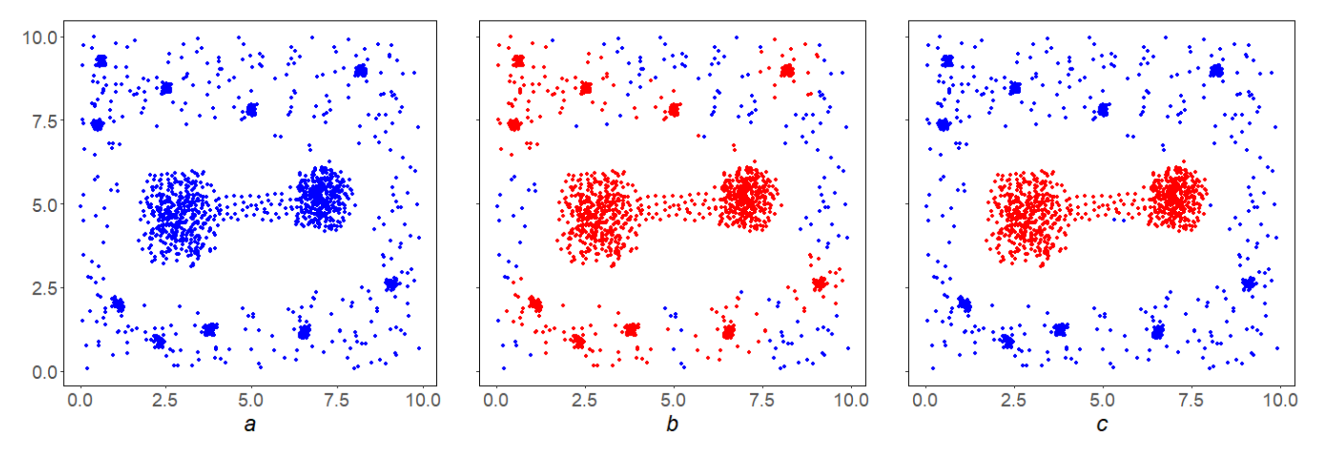
Example 8.

The dumb-bell shaped in Figure 10a has a monolithic but weak handle, so MDPS highlights it cleanly (Figure 10c), while SDPS cannot do so (Figure 10b). This example illustrates the independence of the MDPS and SDPS algorithms.

4.3. FDPS Algorithm

The functional version of the DPS algorithm is related to a special r-local density $F=F\left(\nu \right)$, based on function weighting $\nu :X\to {\mathbb{R}}^{+}$:

$$F_A\left(x\right)=\frac{\sum \nu \left(y\right):y\in D_A(x,r)}{|D_X(x,r)|}$$

The FDPS algorithm is the operation of the DPS circuit on F, as described in Definition 6–Section 3.3.3: $\mathrm{FDPS}=\mathrm{DPS}(F,r,\nu ,\beta )$ [24]. It aims at finding subsets in X with r-local high weights $\nu$, and is capable to work on regular spaces and successfully complements the SDPS and MDPS algorithms.

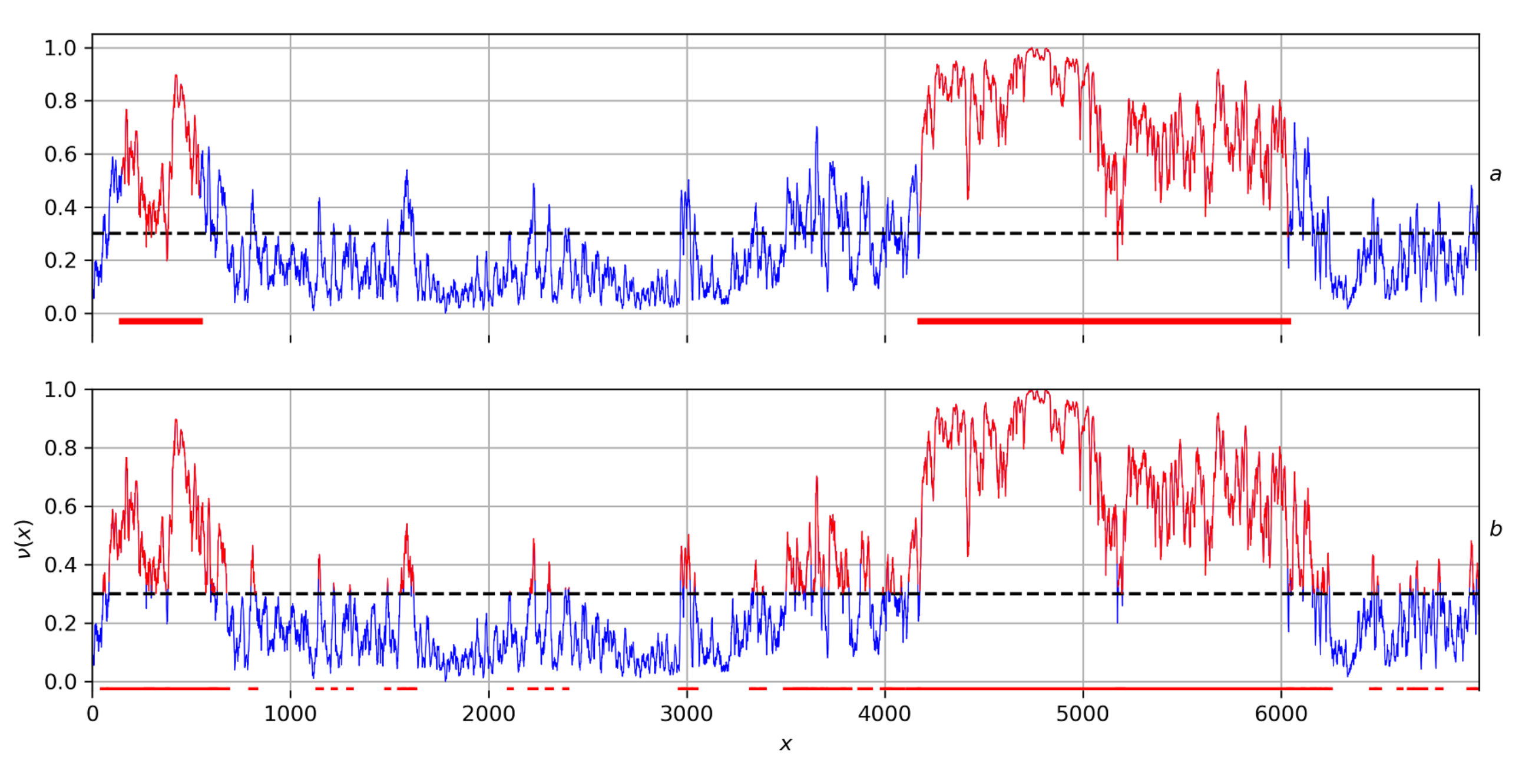
Remark 7.

Weight ν can be thought of as a non-negative relief on X. The FDPS algorithm efficiently searches for the bases of these elevations, which is fundamental in data analysis, in particular in time series analysis (DRAS, FC ARS algorithms etc.) [25].

Example 9.

Figure 11a shows how the FDPS algorithm works: space X in this case is a regular grid on the horizontal axis, where the weight ν of each point$x\in X$is plotted vertically. The result of the FDPS algorithm will be two red bars on the horizontal axis, serving as the bases of the two most significant stochastic ν-elevations on X.

As can be seen from this figure, the FDPS algorithm is stable: it disregards to insignificant drops of contour ν below the set level, as well as to insignificant rises of ν above it. This property of the FDPS explains the solidity of its highlighted elevations and is essential in decision-making issues: the selected areas must be massive and resistant to minor disturbances within them.

To compare, Figure 11b shows a classical selection on grid X with respect to a given level for relief ν. As we can see from the figure, it is unstable, it gives a lot of weak elevations.

4.4. GDPS Gluing: Scheme and Algorithms

Suppose $\mathfrak{P}$ the local property of space X at each of its points x, $P\left(x\right)\ge 0$ its quantification, a $U\left(x\right)=U\left(x\right|P)$ is a subset in the full-sphere $D_{}(x,r)$, where it is reached. In other words, $U\left(x\right)$ is the subset in $D_{}(x,r)$ where the property is most clearly pronounced. It does not necessarily coincide with $D_{}(x,r)$.

Task 1.

For a fixed level of$\alpha$property$\mathfrak{P}$, find the subset$A=X(\mathfrak{P},\alpha )$in X, whose each full-sphere$D_A(a,r)$would have the property$\mathfrak{P}$at each point$a\in A$to the power$\ge \alpha$.

If the quantification of property $\mathfrak{P}$ function P is the density on X Definition 1, then the result of the $\mathrm{DPS}(P,r,\alpha )$ algorithm can be taken as A. Otherwise, we consider a set of local data in X

$$U_{\alpha }=U_{\alpha }\left(P\right)=\left\{U\left(x\right|P):P(x)\ge \alpha \right\}$$

and try to comprehensively fit into $U_{\alpha }$ the global subset $A\subset X$. Let us formulate the requirements for A:

$$\left(P\left(a\right)\ge \alpha \right)\wedge \left(D_A(a,r)\subseteq U\left(a\right)\right)\wedge (\mathrm{difference}U\left(a\right)\backslash D_A(a,r)\mathrm{is}\mathrm{minimal})\forall a\in A$$

(8)

Under the natural assumption of “continuity” of the property $\mathfrak{P}$ we can expect its level of occurrence on $D_A(a,r)$ to be close to $\alpha$.

The mismatch $D_A(a,r)$ with $U\left(a\right)$ in (8) can be understood differently. Some variants of it make it possible to find a solution of (8) using the DPS scheme (Definition 6–Section 3.3.3) with respect to densities specifically constructed by covering $U_{\alpha }$. Let us focus on one of them.

The initial space Y will carry the covering $U_{\alpha }$:

$$Y=Supp{U}_{\alpha }=\left\{x\in X:P\left(x\right)\ge \alpha \right\}$$

The difference in (8) is expressed through the intersection and induces a density G on Y:

$$G_B\left(y\right)=\frac{|D_B(y,r)\cap U\left(y\right)|}{\left|U\right(y\left)\right|}y\in Y,B\subseteq Y$$

(9)

The density G is normalized: $G_B\left(y\right)\in [0,1]$, and its level $\gamma$ is the proximity index in (9).

The dependence $P\to G\left(P\right)$ (9), connecting with the DPS scheme (Definition 6–Section 3.3.3), leads to another dependence $P\to \mathrm{DPS}\left(G\right(P\left)\right)$, which we designate as GDPS and will be understood like $\mathbb{DPS}$ Remark 2 and DPS Remark 3 ambiguously:

• as a schema if we are talking about a dependency given above;
• as the GDPS algorithm when it comes to the operation of the DPS scheme (Definition 6–Section 3.3.3) on density $G\left(P\right)$ with parameter $\gamma$: $\mathrm{GDPS}=\mathrm{DPS}(G,\gamma )$. Its $\mathrm{GDPS}\left(Y\right)$ result solves problem Task 1 by “gluing” local data $U_{\alpha }$ in a certain way. This explains the name of the algorithm (gluing).

If the quantification of P property $\mathfrak{P}$ is the density on X, then the space Y is the first $\alpha$-hull $X^1\left(\alpha \right)$ of space X. The first solution Task 1 (let us call it “a strong one”) is the operation of SDPS on X with respect to P with level $\alpha$. It may differ from the second solution Task 1 (let us call it “a weak one”), which represents the operation of GDPS.

The point is that the SDPS algorithm in its interception on $X^1\left(\alpha \right)$ is guided primarily by preserving the density level $\alpha$, while the GDPS algorithm seeks to preserve the proximity level $\gamma$ on $X^1\left(\alpha \right)$. The weak version is more versatile, since the quantification of P property $\mathfrak{P}$ shall not be necessarily the density on X and it is also more “save” when carving. Therefore, it is the GDPS algorithm that will be part of the DPS-scheme Definition 6–Section 3.3.3 operation when the property $\mathfrak{P}$ represents a local linearity in X.

Let us explain the above on two examples relating to the density $S=S(q,p)$. In this case, the property $\mathfrak{P}$ will be the r-local “space count”, and S will be its formal expression. Since S is a density Definition 1, this Task 1 has two possible solutions: a strong and weak one. The basis for these is the space $Y=X^1(S,\beta )$—the first iteration of the initial space X of relative density S for the level of extremeness $\beta$.

The strong solution is the result of the SDPS algorithm on X with parameter $\beta$ (a subset of $\mathrm{SDPS}(X,\beta ))$ in Y. The weak solution is the result of the GDPS algorithm in this setting, i.e., the result of a DPS-scheme with density $G=G(S,\beta )$ constructed on the basis of local data $U(S,\beta )=\{D_X(y,r):y\in Y=X^1(S,\beta )\}$:

$$G_B\left(y\right)=\frac{|D_B(y.r)\cap D_X(y,r)|}{|D_X(y,r)|}$$

and a given level of proximity $\gamma$ (a subset of $\mathrm{DPS}(G,\gamma )\subseteq Y$).

4.5. LDPS Algorithm

We believe that the initial FMS lies in the Euclidean plane. It is convenient to designate it by Q rather than X for reasons that will be clear below. In this paragraph we implement in detail the previous scenario for the local linearity property in Q. The result of this work done will be the LDPS algorithm from the series of DPS-algorithms, aimed at finding global linear structures in Q.

4.5.1. Initial Data and Designations

$\Pi$ is the universe plane

• $xOy$—fixed orthogonal coordinate system on $\Pi$,
• $x_{\phi }{O}^{*}{y}_{\phi }$—loose orthogonal coordinate system on $\Pi$, obtained by moving coordinate origin O to point $O^{*}=(x^{*},y^{*})$ and turning the axes $x_{\phi },y_{\phi }$ by the angle $\phi \in [0,\pi ]$,
• Relation of coordinates

  $$\begin{array}{c}{x}_{\phi }=cos\phi (x-x^{*})+sin\phi (y-y^{*})\hfill \\ y_{\phi }=-sin\phi (x-x^{*})+cos\phi (y-y^{*})\hfill \end{array},$$
• Q is a finite-state array in $\Pi$: $Q=\left\{q\right\}=\left\{q_i{|}_{i=1}^N\right\}$,
• $r=r_s\left(Q\right)$, $s<0$ (5),
• $\mathfrak{L}$—the property of local linearity in Q.

4.5.2. Quantification $\mathfrak{L}$

Let $q^{*}$ be an arbitrary fixed point in Q, $\phi$ arbitrary angle in $[0,\pi ]$. Let us move to the coordinates $x_{\phi }{q}^{*}{y}_{\phi }$ and we denote the “square” neighborhood Q in $q^{*}$ of radius r$K_Q\left(q^{*}\right|\phi ,r)$:

$$K_Q\left(q^{*}\right|\phi ,r)=\left\{q\in Q:|x_{\phi }\left(q\right)|\le r,|y_{\phi }\left(q\right)|\le r\right\}.$$

The additional parameter “height” $h\in (0,r]$ enables defining the corridor $K_Q\left(q^{*}\right|\phi ,r,h)$ in $K_Q\left(q^{*}\right|\phi ,r)$

$$K_Q\left(q^{*}\right|\phi ,r,h)=\left\{q\in Q:|x_{\phi }\left(q\right)|\le r,|y_{\phi }\left(q\right)|\le h\right\}.$$

Using $K_Q\left(q^{*}\right|\phi ,r)$ and $K_Q\left(q^{*}\right|\phi ,r,h)$ we define a measure of local linearity $L_Q\left(q^{*}\right|\phi ,r,h)$ of space Q at point $q^{*}$ to the direction $\phi$ as the density $K_Q\left(q^{*}\right|\phi ,r,h)$ against the background of $K_Q\left(q^{*}\right|\phi ,r)$ by serial relation:

$$L_Q\left(q^{*}\right|\phi ,r,h)=\frac{|K_Q\left(q^{*}\right|\phi ,r,h)|}{K_Q\left(q^{*}\right|\phi ,r)|}.$$

Maximum value

$$L_Q\left(q^{*}\right|r,h)=\underset{\phi }{max}{L}_Q\left(q^{*}\right|\phi ,r,h)$$

will be considered a quantitative expression of the property $\mathfrak{L}$ for Q in $q^{*}$, and the neighborhood of $U(q^{*},\mathfrak{L})$ is the best corridor $K_Q\left(q^{*}\right|r,h)$ where this maximum is reached.

For geometrical reasons, the relation $h{r}^{-1}\in (0,1/2]$ must be considered as satisfied.

4.5.3. Search for Global Linear Structures

A quantification L of the property $\mathfrak{L}$ is made. Hence, it is possible to involve a GDPS scheme based on L for the weak solution of Task 1 in this case, which leads to the $\mathrm{GDPS}(P,\alpha ,\gamma )$ algorithm, where $\alpha$ is the expression level of property L and $\gamma$ is its representativity degree.

Research shows that in the generic case its result Z on space $Y=Q^1(L,\alpha )$ needs additional filtering, which is done by the MDPS algorithm with a solidity level $\epsilon$. Its result $\mathrm{MDPS}(Z,\epsilon )$ is considered final in the search for linear structures within the space.

The LDPS algorithm is the described superposition of GDPS and MDPS:

$$Q\to Q^1(L,\alpha )=Y\to \mathrm{GDPS}(Y,\gamma )=Z\to \mathrm{MDPS}(Z,\epsilon )=\mathrm{LDPS}\left(Q\right).$$

Its parameters will be (parameters L) + (parameters M) + $(\alpha ,\gamma ,\epsilon )$, and the result is the global linear structures in Q relative to them.

The LDPS algorithm has four stages:

• the first of them with the selected parameters of local linearity r and h constructs its quantification $L_Q\left(q\right|r,h)$ at each point q of space Q, and the best corridor $K_Q\left(q\right|r,h)$, where the estimate $L_Q\left(q\right|r,h)$ is reached;
• the second stage includes constructing the basis for application of the GDPS scheme, namely coverage $U_{\alpha }\left(L\right)=\{K_Q\left(q\right|r,h):L_Q\left(q\right|r,h)\ge \alpha \}$ for a given level of local linearity $\alpha$;
• the third stage is GDPS scheme working on $U_{\alpha }\left(L\right)$ data. Its result will represent linear structures in Q. On space

  $$Y=Supp{U}_{\alpha }\left(L\right)=\{q\in Q:L_Q\left(q\right|r,h)\ge \alpha \}$$

  a measure $G=G\left(U_{\alpha }\left(L\right)\right)$ is constructed (9)

  $$G_B\left(y\right)=\frac{|D_B(y,r)\cap K_Q\left(q\right|r,h)|}{|K_Q\left(q\right|r,h)|}.$$

  The result will represent the raw linear structures on Q;
• the fourth stage is their filtering by solidity using the MDPS algorithm with a level of $\epsilon$.

In conclusion, we will address the operation of the LDPS algorithm on two arrays, while the operation in the first instance will be explained in detail, and in the second instance only the result is shown.

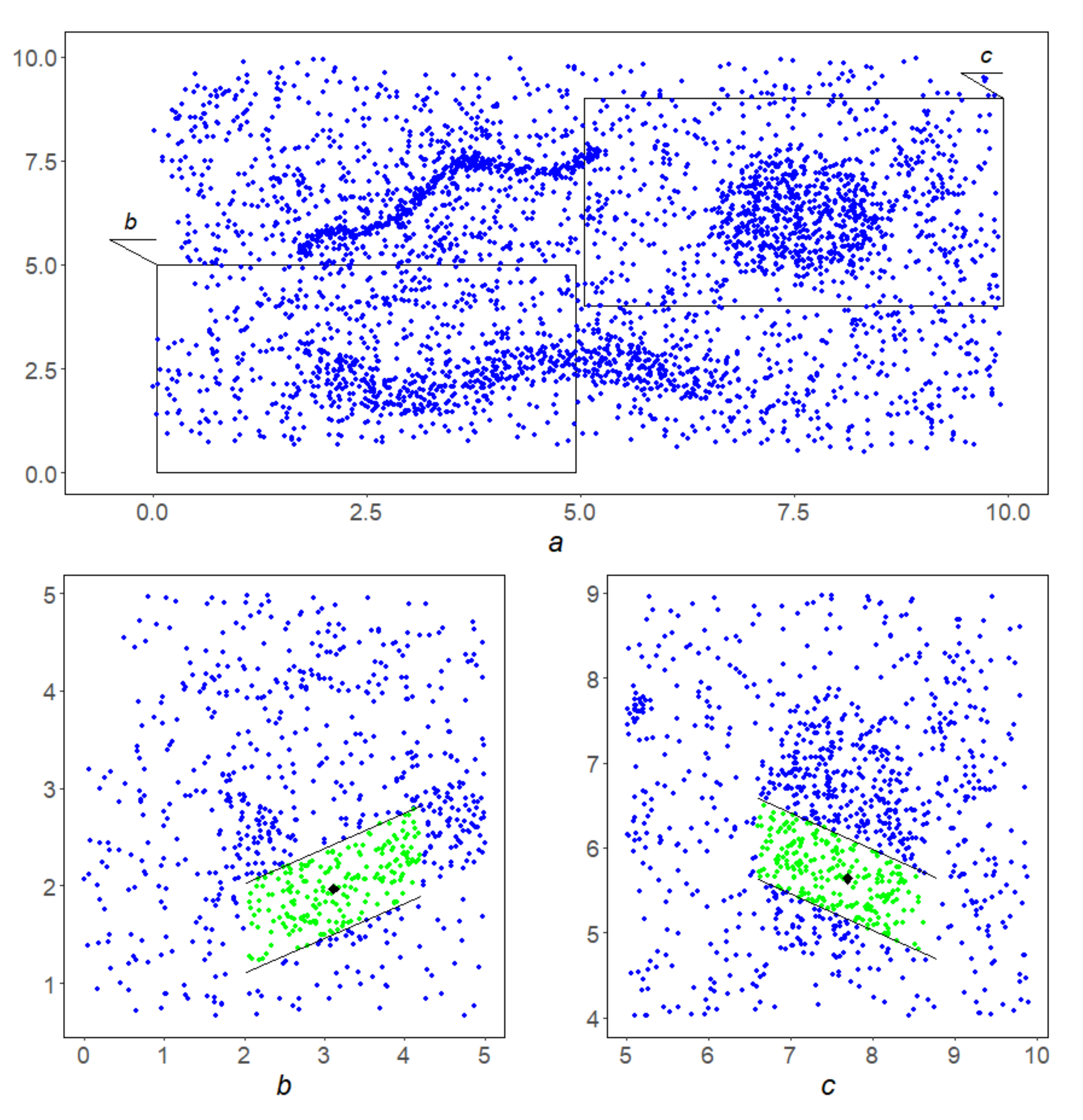
Example 10.

The initial array Q is shown in Figure 12a

• At the first stage with the chosen parameters at each blue point q a linear corridor$K_Q\left(q\right|r,h)$is constructed with parameters$r=1.09$and$h=0.44$, then its separability$L_Q\left(q\right|r,h)$is calculated. Figure 12b,c show corridors in green with centers at black points. Their separability equals to$0.64$ and $0.5$, respectively. In the second instance, it proves to be insufficient to overcome the second stage.
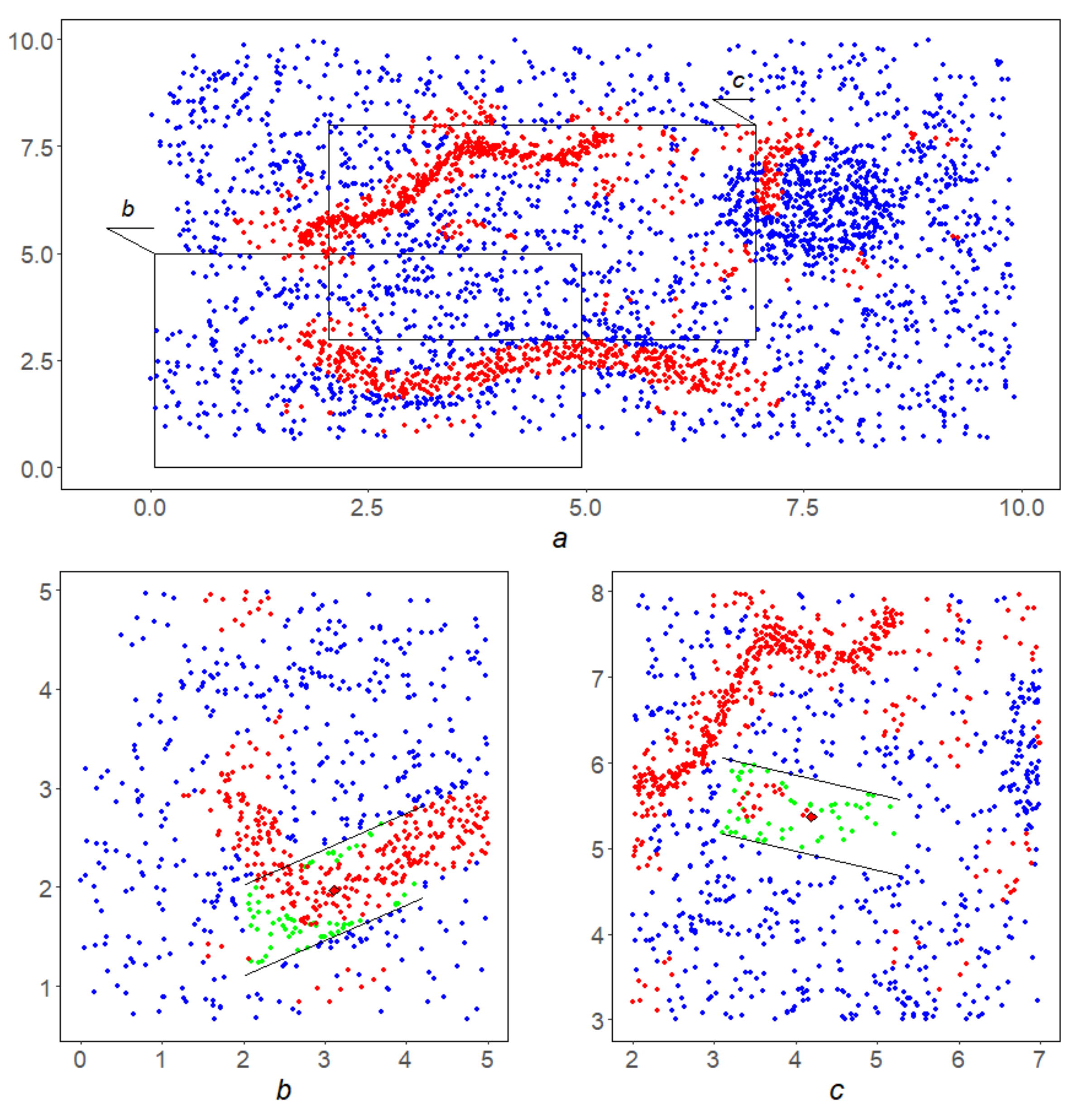
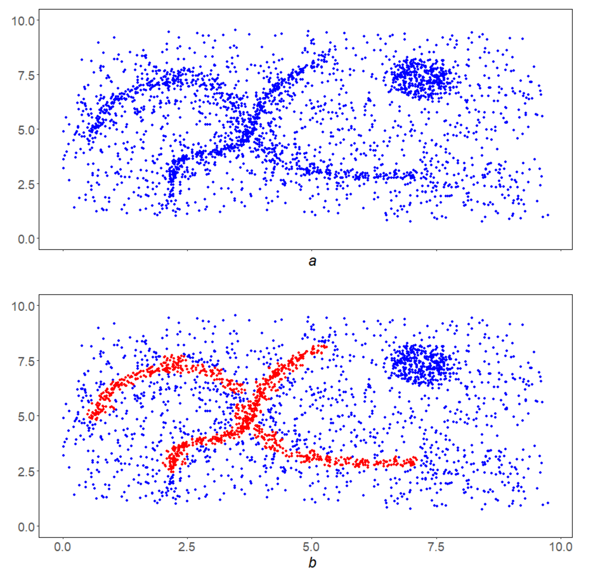
• Second stage. The separability level α is assumed to be$0.6$. Figure 13a shows the points y in red, that passed this selection and formed the basis Y—the first half for application of the GDPS scheme. The second half GDPS scheme: corridors$K_Q\left(q\right|r,h)$are shown for the already familiar point on the left (Figure 13b) and at some point on the right (Figure 13c). It can be seen from the figures that the relative density of red dots in the left corridor is higher than in the right one. This circumstance will help the left point overcome the third stage and move into the lower linear structure, while the right point will not stand the test with GDPS operation and will not be included in the final result.
• Third scheme. The GDPS scheme operation on the red points from the Y. Its result Z is shown in Figure 14a. It needs to be filtered.
• Fourth stage. This is implemented by the MDPS algorithm on Z. The result is shown in Figure 14b. Figure 14c,d show how the well-known DBSCAN [18] and OPTICS [19] algorithms operates in this instance.

Example 11.

The initial array is shown in Figure 15a, and the LDPS result is shown in Figure 15b.

5. Discussion

This paper addressees the study of stationary data arrays, which are finite sets in multidimensional spaces, using the DMA methods by means of clustering.

A complex local condition is a conjunction of the conditions of local linearity and local representativeness. Local linearity: each point L has a linear corridor containing it that is dense against the background of Q, i.e., each point $q\in L$ on the plane has a rectangle $K\left(q\right)$ centered at q, which is a local corridor for L, and the intersection $K\left(q\right)\cap Q$ is dense against the background Q. Local representativeness: the intersection $K\left(q\right)\cap$L is dense in $K\left(q\right)\cap Q$.

The global condition for L consists of the requirement that L has no isolated points, i.e., in its discrete perfection. The detection of local linearity in the implementation of LDPS consists of a direct check for all points of the original space Q of this property. Analytical procedures are available to reduce routine calculations. In addition, in the future, we propose to modify the algorithm so that the dimensions of the corridors generally change from point to point.

The points in Q that pass the local linearity test form a subset of Y—the first approximation in Q to linear structures. We checked the linear representativity on Y in the LDPS algorithm as an implementation of the DPS scheme with respect to the special density G (clause 4.5.3). In the future, we plan to implement other variants of the LDPS algorithm based on a change in the interpretation of linear representativeness.

Studies have shown that, among the subset of points $Z\subset Q$ that have passed the local test for representativeness, there may be isolated points. The global condition in LDPS eliminates this drawback: its check for Z is also organized as an implementation of the DPS scheme with respect to the density “monolithicity” (MDPS algorithm). The points that pass the global test will be the result of applying the LDPS—that is, the union of all linear structures in Q.

In the general case, the set of linear structures L is divided into connected components. For example, in the examples given in Figure 14b and Figure 15b, two connectivity components are obtained. In the first example, the components of connectivity should be considered independent linear structures, and in the second example, as part of a single whole. In the future, we plan to introduce an additional procedure for joining the results of applying the LDPS algorithm in order to obtain global linear structures in the original space Q.

Comparison of the LDPS algorithm with the well-known new generation cluster analysis algorithms DBSCAN and OPTICS, as well as with the previously created DMA clustering algorithms, shows that the LDPS algorithm is not inferior to them in detecting clumps; however, at the same time, it is more focused on recognizing clumps with a linear structure.

The implementation of the formal approach as shown in the article can be very effective in various fields of Earth sciences where linear structures play a special role in the investigation of spatial patterns of geographical location and geometric configuration of natural objects. This is vital when solving the issue of predicting the isolation properties of the geological environment for the preparation of a rationale for the geodynamic stability over long periods of time (ten to one hundred thousand years), arising in the selection of HLRW disposal sites. Further to this task, the algorithm can apply to the analysis of elongated artificial structures, such as road networks, etc.