Geometry-Based Preliminary Quantification of Landslide-Induced Impulse Wave Attenuation in Mountain Lakes

Abstract

In this work, a simple methodology for preliminarily assessing the magnitude of potential landslide-induced impulse waves’ attenuation in mountain lakes is presented. A set of metrics is used to define the geometries of theoretical mountain lakes of different sizes and shapes and to simulate impulse waves in them using the hydrodynamic software Flow-3D. The modeling results provide the ‘wave decay potential’, a ratio between the maximum wave amplitude and the flow depth at the shoreline. Wave decay potential is highly correlated with what is defined as the ‘shape product’, a metric that represents lake geometry. The relation between these two parameters can be used to evaluate wave dissipation in a natural lake given its geometric properties, and thus estimate expected flow depth at the shoreline. This novel approach is tested by applying it to a real-world event, the 2007 landslide-generated wave in Chehalis Lake (Canada), where the results match well with those obtained using the empirical equation provided by ETH Zurich (2019 Edition). This work represents the initial stage in the development of this method, and it encourages additional research and modeling in which the influence of the impacting characteristics on the resulting waves and flow depths is investigated.

1. Introduction

Landslide-induced impulse waves in lakes are gaining interest in the scientific community due to the hazards they pose to people living or recreating along their shorelines and to dams and other infrastructure [1]. Additionally, climate change is driving rapid geomorphological changes in high mountains, which may increase the likelihood of landslides into mountain lakes. Rapid thinning and retreat of glaciers and an increase in heavy rainfall events can destabilize slopes adjacent to water bodies [2,3,4,5].

In December 2007, a 3-Mm³ rock avalanche entered the Chehalis Lake (Canada), generating an impulse wave that destroyed forest and campgrounds along the shoreline and achieved a maximum run-up of 37.8 m above average lake level [6,7]. In July 2014, a 10-Mm³ rockslide collapsed into Askja Lake (Iceland) from its rimming caldera and generated a wave that propagated >3 km across the lake with localized run-ups of up to 60–80 m [8]. In October 2015, a 50-Mm³ landslide collapsed into Taan Fiord (Alaska), inducing one of the largest landslide-induced waves ever recorded, with a maximum run-up of 193 m on the slope facing the landslide; the wave traveled >17 km down the fiord, devastating forests and eroding soil and sediments along its path [5,9]. In June 2017, an impulse wave generated by a 50-Mm³ subaerial rockslide into Karrat Fiord on Greenland’s west coast killed four people and destroyed 11 buildings in the village of Nuugaatsiaq, 32 km from its source, and flooded other settlements along the coast [10]. These events are just a small subset of all the subaerial landslides known to have generated impulse waves around the world [1].

Different methods, including scaled physical tests, field investigations, and numerical models are used to investigate aspects of this phenomenon, including landslide behavior, landslide–water interaction, and wave formation, propagation, and inundation. The effect of basin geometry on wave propagation has been experimentally and numerically investigated [11,12,13]. Researchers have also analyzed wave dispersion and related wave decay. Ruffini et al. [14] state that wave decay results from (i) frequency dispersion, (ii) bottom friction, (iii) lateral spreading of the water, and (iv) breaking of waves during generation and propagation. According to those authors, an increase in the lateral angle of the basin leads to a decay of solitary waves. The effect of lateral energy spread on wave amplitude is larger in a 3D basin-type geometry than the effect of frequency dispersion in a 2D flume-type geometry.

To virtually reproduce wave dynamics generated by an impact, researchers have used several different numerical approaches, notably non-linear shallow water equations (NSWE), Reynolds-averaged Navier–Stokes equations (RANS), and smoothed particle hydrodynamic methods (SPH) [13]. These approaches have been used to retrospectively investigate specific landslide-induced impulse wave events, typically with much success. However, such modeling approaches, when used in assessments of possible future events, are compromised by cost, computational time, the considerable amount of data required for model calibration and validation, and the absence of run-up and inundation evidence typically used to fine-tune model parameters

Other methods, such as generic empirical equations, can be used for preliminary assessment of the potential impact of landslide-generated waves and to guide decisions on the need for further investigations. Empirical relationships, commonly based on field-measured wave impacts of historical events or scaled physical experiments, are used to determine wave characteristics. The analytical equations of Heller et al. [15], Heller and Hager [16], and Evers et al. [17] were developed to assess impulse waves in artificial water basins impounded by dams but are also applicable to natural lakes. Their equations, and the 3D approach employed in them, provide estimates of wave characteristics while accounting for variable propagation angles and travel distances, thus covering a wide range of water-basin geometries. The main inputs into their set of equations are landslide properties and a representative lake depth. Their workflow provides the first estimate of impulse wave celerity and waves run-up.

Strupler et al. [18] suggest a classification of mountain lakes based on their impulse wave potential, which they derived from both subaerial and subaqueous mass movements at Swiss perialpine lakes >1 km². Their method relies on parameters calculated from digital elevation data (using geospatial software), for instance, topographic surfaces and bathymetry, together with seismologic data (e.g., the local acceleration), considered as an external factor for landslide initiation. They argue that lakes in the Alps have a high potential for impact by subaerial or subaqueous mass movements due to the surrounding steep slopes and fiord-like morphology of the lake basins compared to perialpine lakes. The latter lakes have a lower potential for subaerial mass movement, but a larger potential to inundate surrounding areas because of the typically lower relief surrounding them.

Despite the simplicity of diverse approaches available in the literature, there are some limitations, such as the technical knowledge required to properly use these tools and limited availability of high-resolution geospatial data—particularly bathymetry—which may necessitate the use of lower-quality digital elevation data. In this paper, a simple alternative method, based on lake shape and extent, for estimating impulse wave propagation in mountain lakes (Figure 1) is presented. The method has a short workflow based on analytical equations derived from the analysis of wave characteristics and estimated using hydrodynamic numerical models in Flow-3D for theoretical mountain lakes. A fixed impact volume is used to induce the impulse wave. In comparison to other approaches, the equations are easy to apply. The variables required are the geometric characteristic of lakes; no specifics of the impacting landslide are needed.

We describe the near-shore impulse-wave magnitude in terms of flow depth at the shoreline. This novel approach enables rapid, resource-efficient, preliminary investigations that may be required to identify basins of particular concern or high risk and to justify more detailed data collection and analysis. An Excel spreadsheet, as a Computational tool, comprising the presented workflow is available in the Supplementary Materials.

2. Materials and Methods

Data used in this study are derived from 56 subjectively selected alpine and perialpine lakes in the Alps region (table in Supplementary Materials). All of the lakes are bordered by slopes that could potentially generate subaerial mass movements. Characteristics of most lakes—water volume (V_w), lake area (A), width (W), length (L), and mean and maximum water depth (d_w and D_w)—are already available from the literature and diverse online sources [23,24,25,26]. Bathymetric data for some of the lakes were provided by the Sedimentary Geology Working Group at the University of Innsbruck (see a listing in the table in the Supplementary Materials [19,20]) and the Swiss Service (Federal Office of Topography-swisstopo), enabling a more accurate geometric data calculation utilizing the Raster Layer Statistics and Raster Surface Volume tools in QGIS v3.16.

A classification scheme is developed to group and discriminate the geometries of the 56 lakes in the dataset (Section 3). Frequency analyses are performed to identify the most common lake metrics and to combine them to produce a representative range of theoretical lake-basin shapes for use in subsequent numerical modeling. These theoretical lake basins are generated as 3D solid bodies and exported to stereolithography (STL) files using Rhinoceros 6 software (see Supplementary Materials).

Numerical models are implemented in the finite-volume-based for computational fluid dynamics (CFD) software Flow-3D v11.1 [27,28,29,30]. This software simulates two-fluid problems, where all velocity components (u, v, w) are computed in the 3D domain using RANS equations [31] in combination with the volume-of-fluid method [29,32], and adopting the fractional-area/volume-obstacle-representation [33]. To compute turbulence and viscosity processes in Flow-3D, the renormalized group model-based k-epsilon turbulence model [34] is applied to create a fluid–fluid coupled model of the impulse wave. This model uses statistical formulations to compute the turbulent kinetic energy dissipation rate [35,36,37]. A Newtonian-like fluid (see Section 4), featuring a higher density compared to the still-water density, is adopted to simulate the impacting volume [38]. Modeled free-water-surface elevations, wave-crest elevations in open water, and flow depth at the lake shoreline are post-processed in FlowSight v11.1 [27]. Finally, correlation matrices between the numerical input parameters and the modeling results are generated to establish a relationship that can be used to assess potential impulse waves in natural mountain lakes.

3. Classification and Frequency Analysis of Alpine Lake Geometries

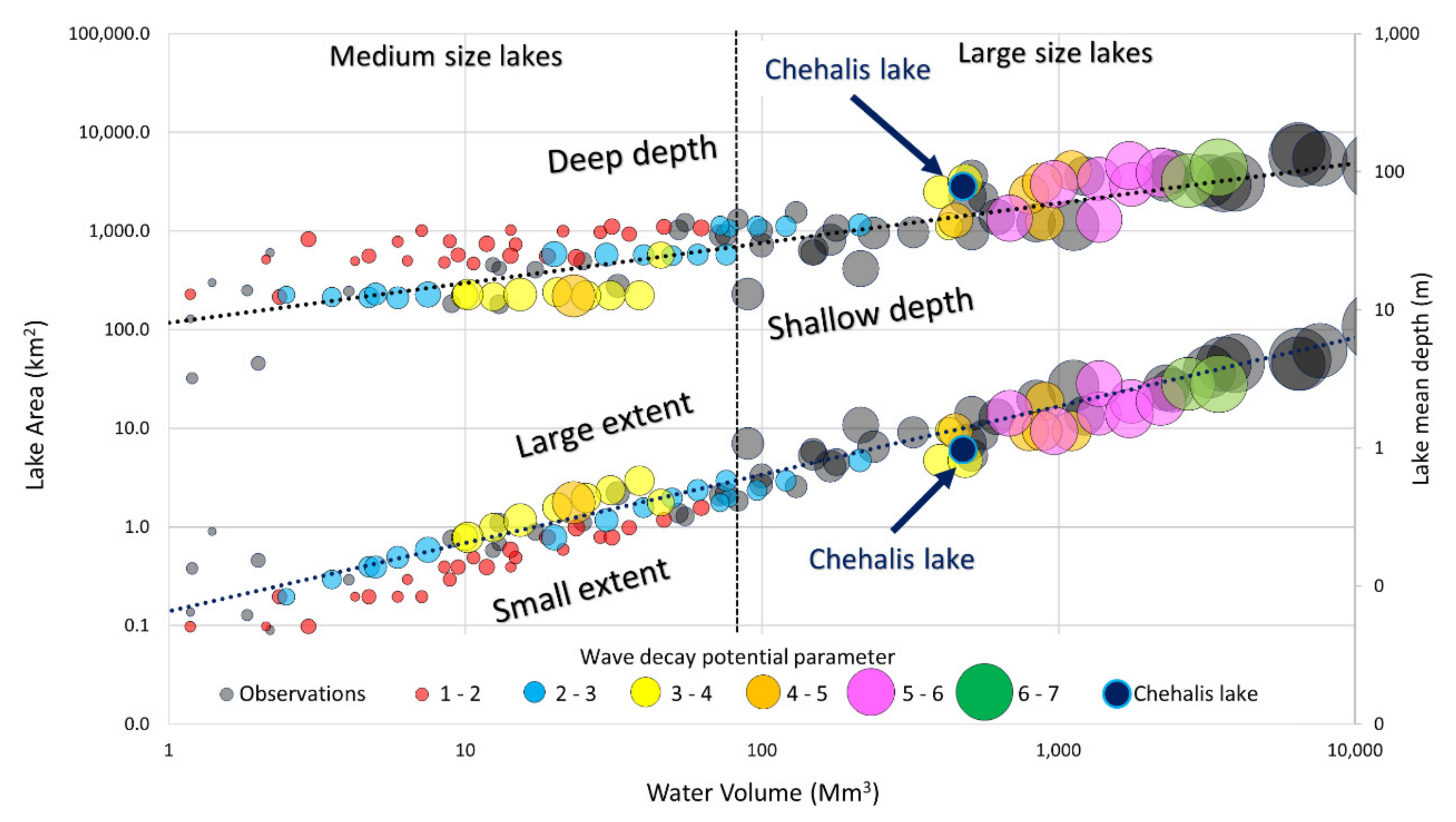
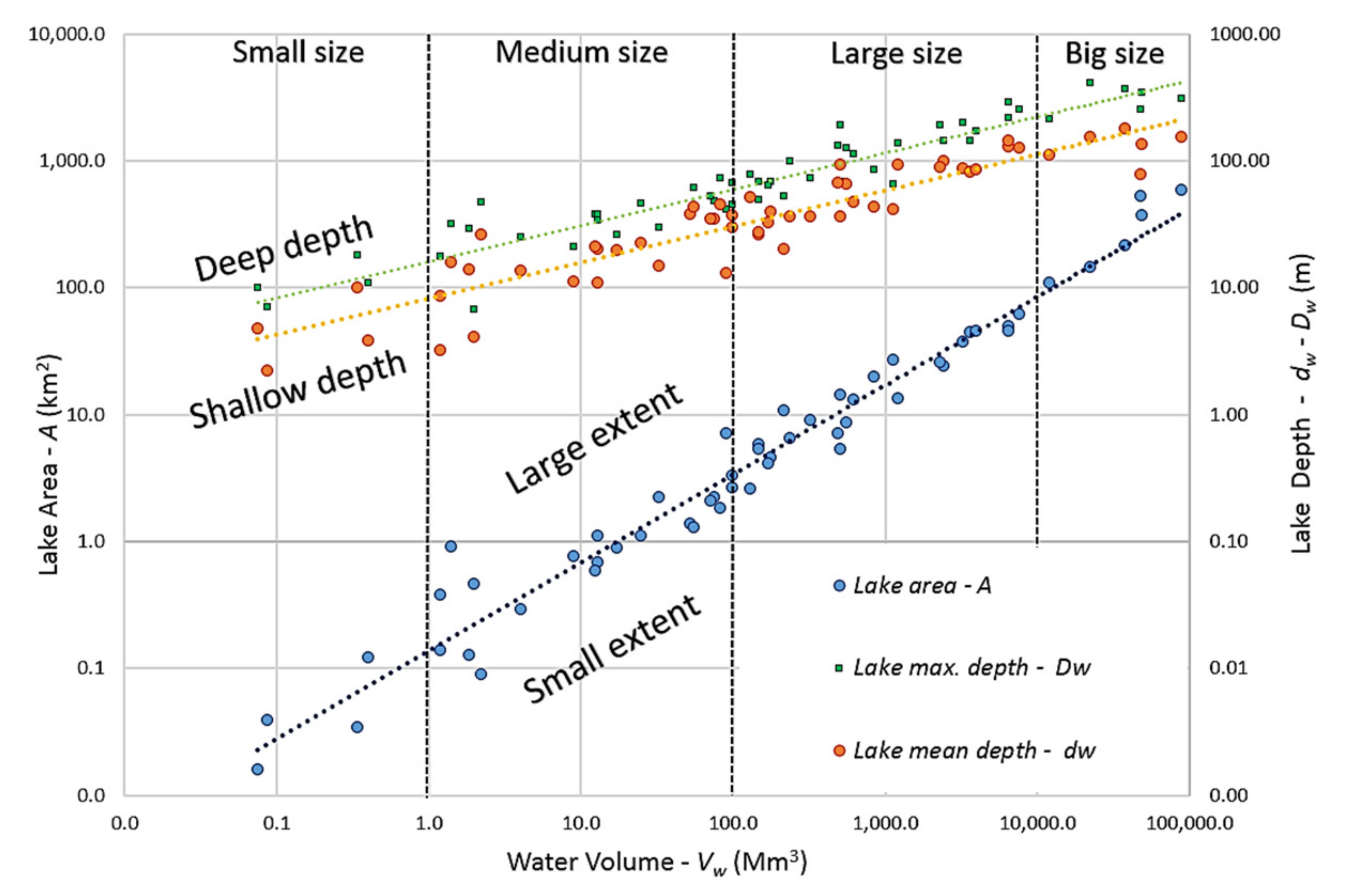
A classification of the considered alpine lakes is shown in Figure 2. The figure shows the relationships between water volume (V_w) and lake area (A) and between water volume and mean (d_w) and maximum (D_w) lake depth (each data point represents a single lake). The data are subjectively grouped and named based on ranges of V_w as follows: small-size lakes (V_w < 1 Mm³); medium-size lakes (V_w 1–100 Mm³); large-size lakes (V_w 100–10,000 Mm³); and very large-size lakes (V_w > 10,000 Mm³).

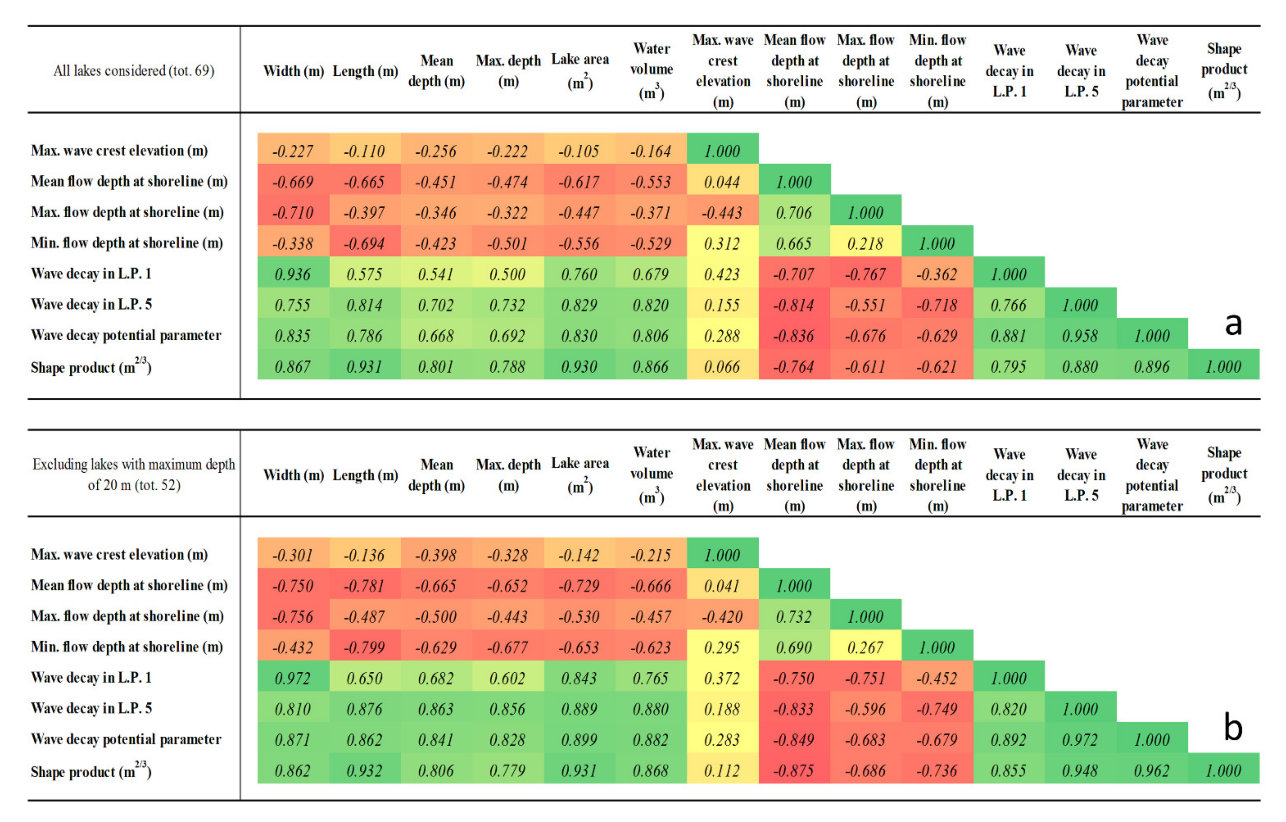
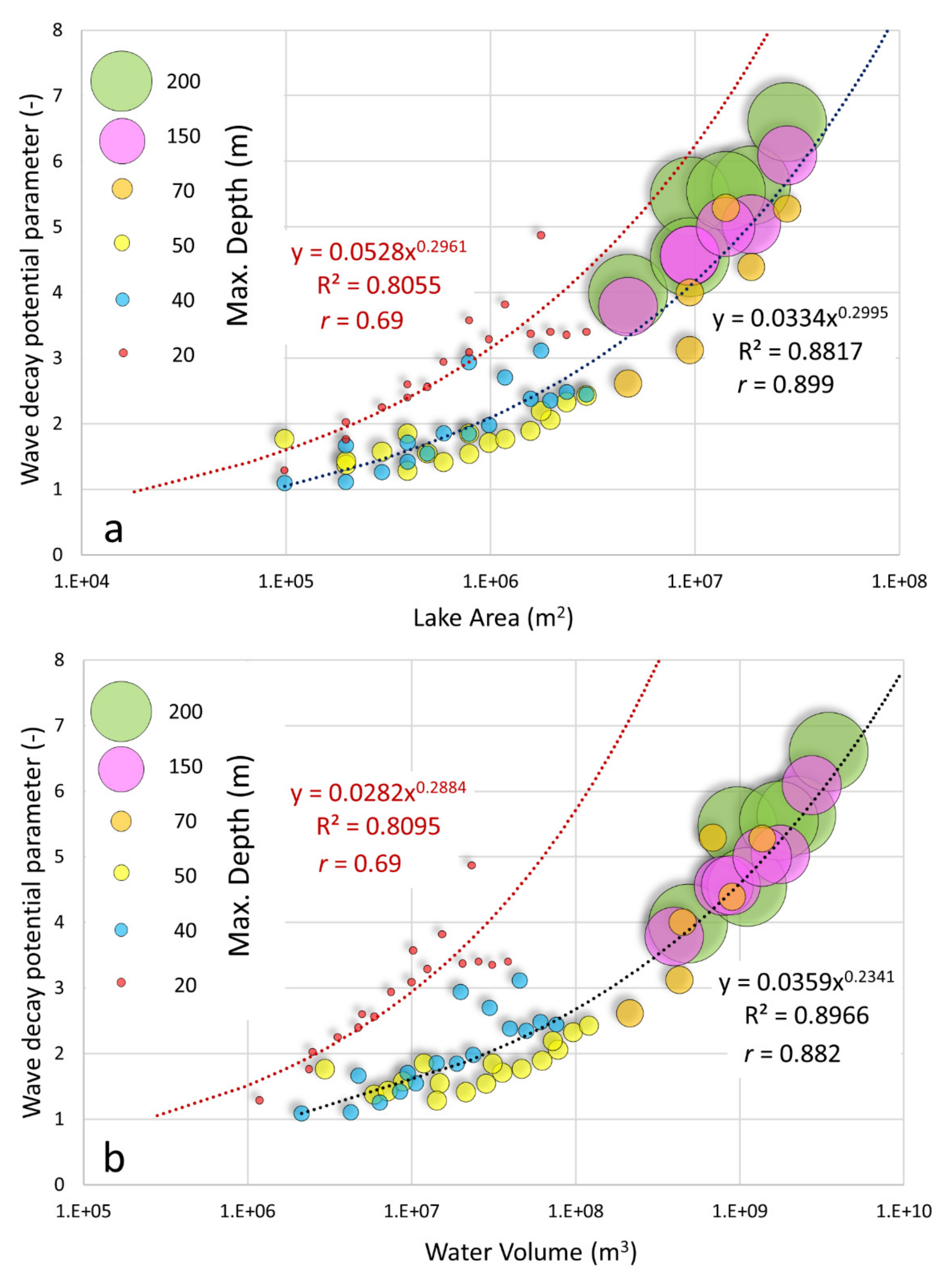
Trendlines in Figure 2 quantitatively describe lake extents and water depths relative to water volume. The higher a lake is above the trendline, the larger the volume-normalized extent or the deeper the volume-normalized depth. Conversely, increasing distance below trendlines indicates a smaller extent or shallower depth relative to lake volume. Among the 56 lakes considered, 42% and 58% have large- and small-volume-normalized extents, respectively; and 53% and 47% have deep and shallow-volume-normalized depths, respectively.

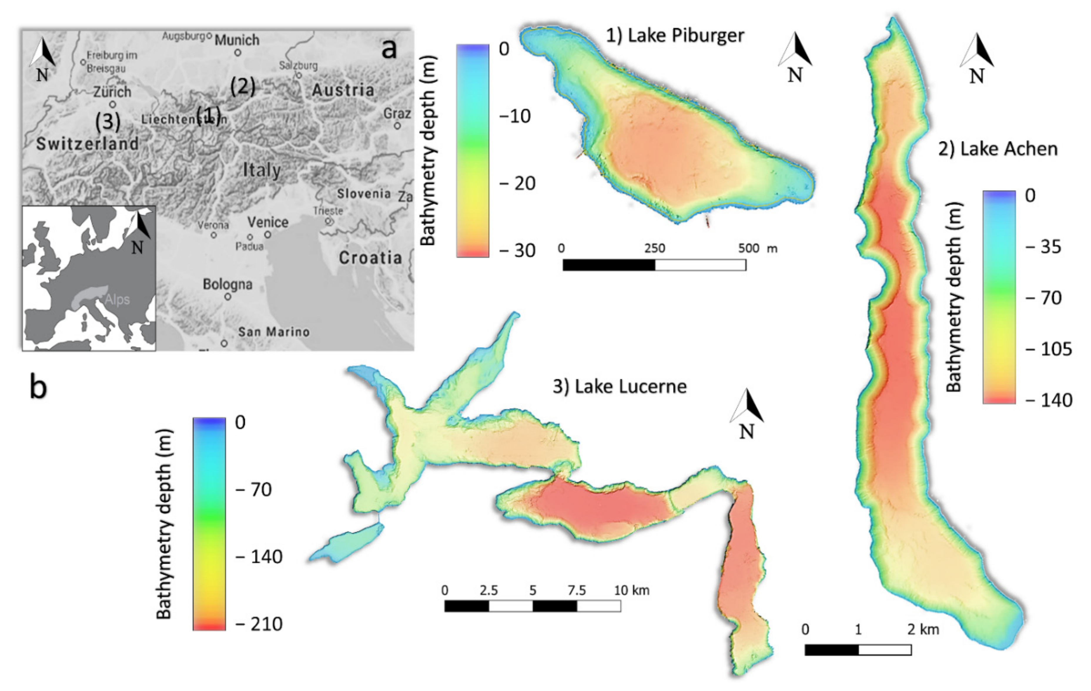
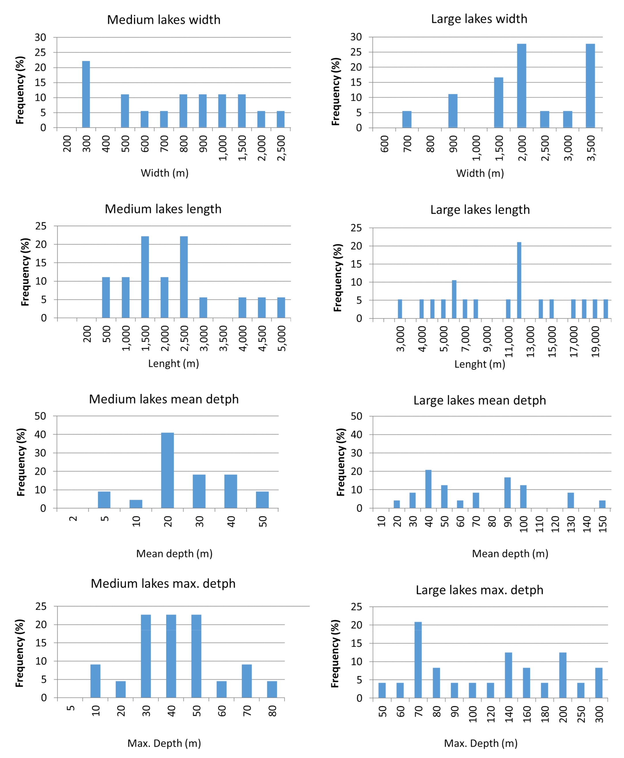
Considering a ratio between L and W, it is possible to differentiate elongate lake shapes (L/W > 1.5, about 60% of them; e.g., Lake Achen in Figure 1) from those that are approximately equidimensional (1 < L/W < 1.5, about 16%). Other lakes (the remaining 24%) have complex shapes, generally comprising sub-basins (e.g., Lake Lucerne in Figure 1). These are mostly large- and very large-size lakes. Given that sub-basins of complex lakes are themselves either medium or large size and that only a few small lakes were identified, the small-size and very large-size lake classes are not considered further in the analysis. Results of a frequency analysis of lake geometrical characteristics for the medium-size and large-size lake classes are shown in Figure 3.

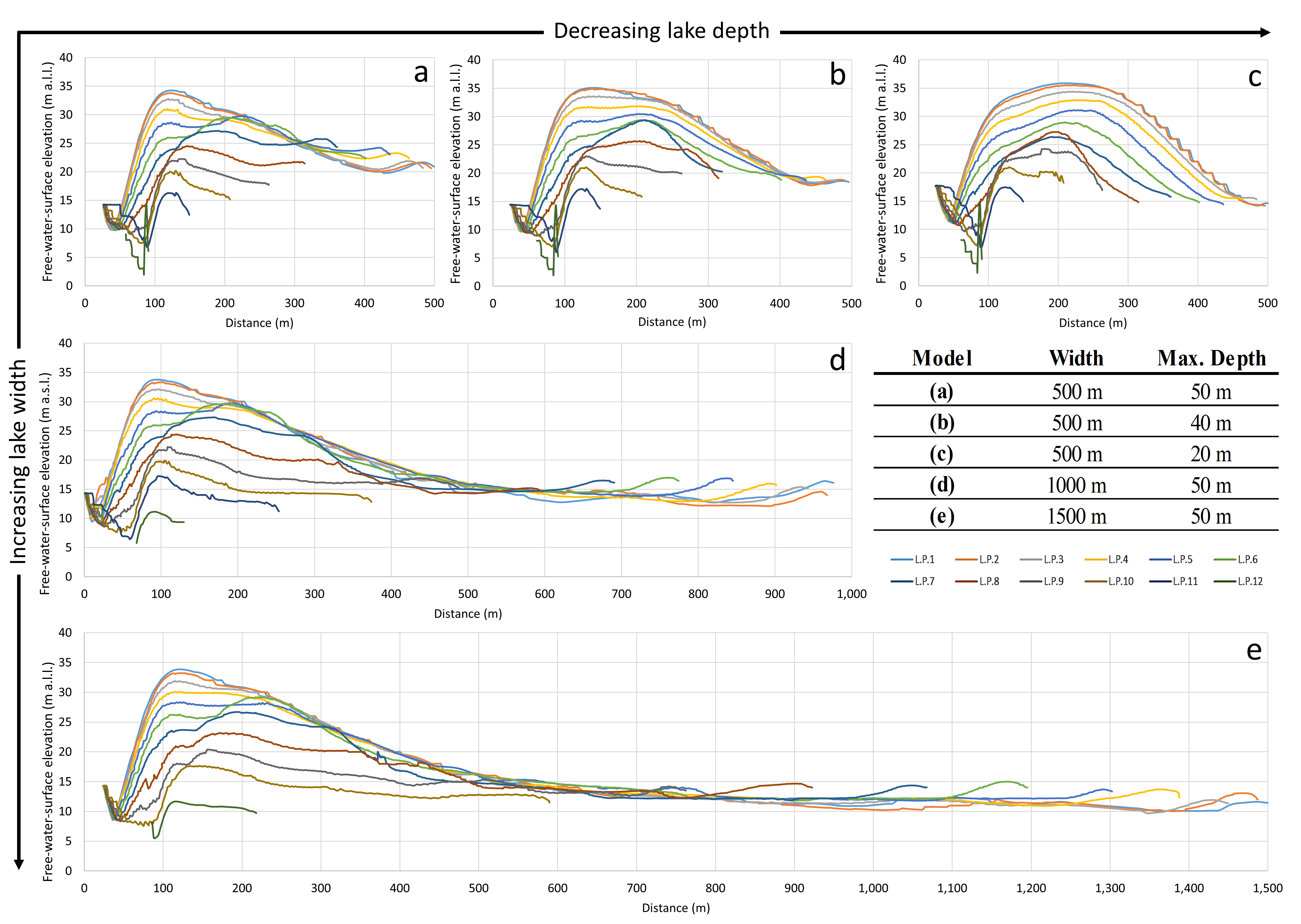
Based on the aforementioned classification, different combinations of parameters are subjectively defined to design theoretical lakes that cover the considerable variability of mountain lake configurations in the Alps.

Table 1. Geometry parameters chosen for the theoretical lakes [lake width (W), length (L), and mean and maximum water depths (d_w and D_w)]. Permutations of these three variables yield a total of 69 lake-basin configurations.

Lake Class	dw–Dw (m)	W (m)	L (m)
Medium size lakes	10–20	250	500
	20–40	500	1000
	40–50	1000	1500
		1500	2000
			2500
Large size lakes	40–70	1000	6000
	80–150	2000	12,000
	100–200	3000

shows the selected values for the two size classes, resulting in 51 combinations for medium-size lakes and 18 for large-size lakes. These 69 theoretical lakes form the basis for the numerical modeling part of this study (both a complete table with related information and STL files are available in the Supplementary Materials).

4. Numerical Model Set-Up

Numerical models are designed to reflect conditions typical of mountain lakes in alpine settings, albeit with some necessary simplifications. Alpine basins, whether small or large, commonly fill topographic depressions with adjacent steep slopes that in many cases are the product of glacial erosion or deposition [39]. Steep slopes are particularly common along valley sides, making subaerial landslides capable of generating impulse waves more likely along lakesides than ends (e.g., [6,39,40]). Consequently, impacting volumes initiated in these environments enter the lake along its sides in all modeled scenarios.

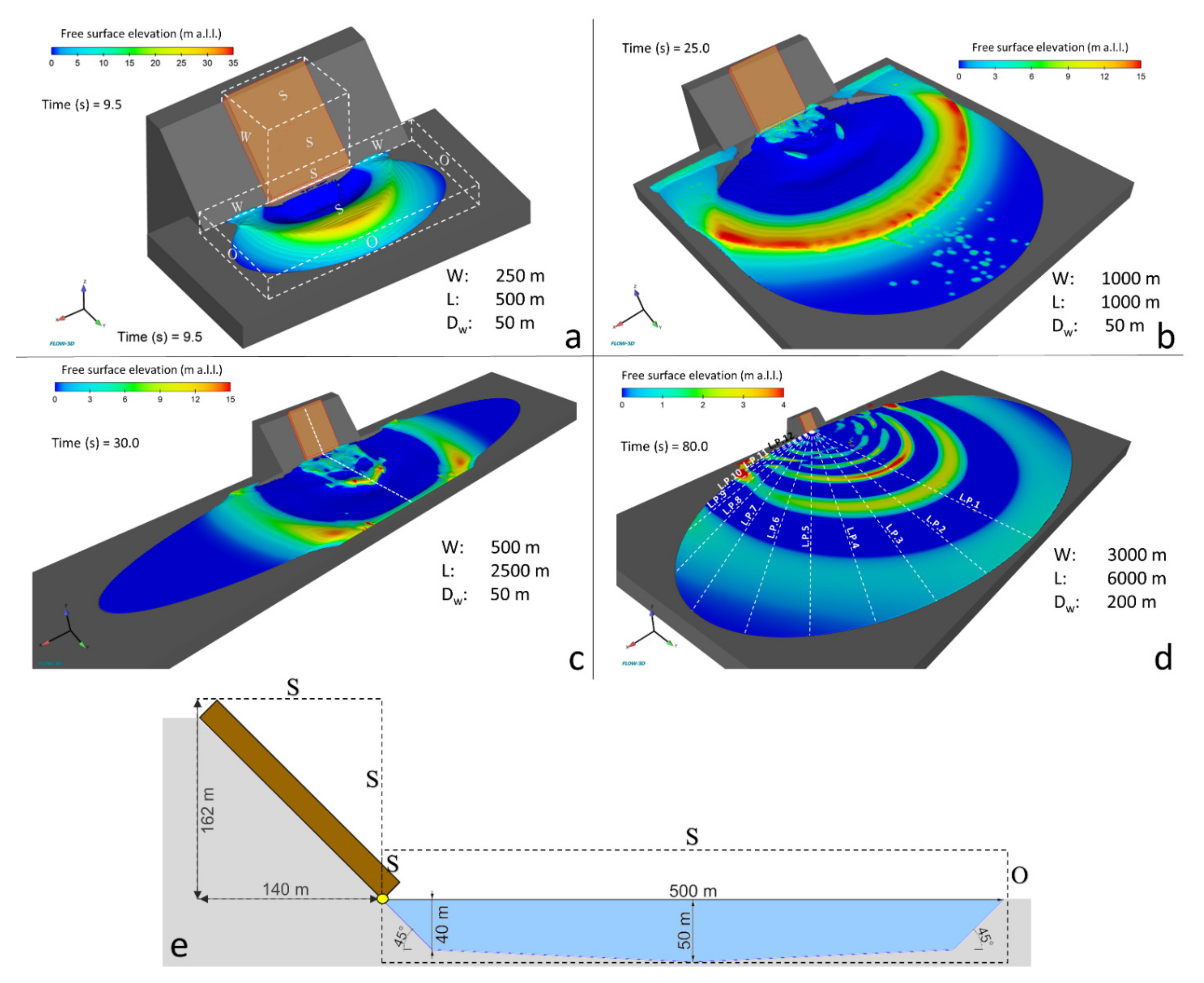
Each numerical simulation considers that same impacting volume for triggering the wave. This lies initially on a sliding surface dipping 45° toward the lake and is represented by a 0.5 Mm³ prismatic fluid body, 20 m thick, 208 m long, and 120 m wide, with a toe position directly above the lake surface (Figure 4). The volume is located mid-way along the side of each theoretical lake.

A bulk material density of 1620 kg m⁻³ is used for the landslide [38]. Additionally, an initial speed of 20 m s⁻¹ at simulation time 0, is arbitrarily set. This, together with volume deformation during the sliding process, results in a maximum speed of 60 m s⁻¹ for the center of mass at the impact in all models, regardless of lake geometry.

For each simulation, the model domain includes the slide area, the entire water body, and the air above it to 40 m above lake level (m a.l.l.). The origin of the system (x,y,z equal to 0) is located midway along the long side of each artificial lake at the middle of the landslide toe (0 m a.l.l.). The maximum depth D_w is located at the center of each theoretical lake (Figure 4e). A mesh block of 120 m × 140 m × 162 m, comprising 2 m × 2 m × 2 m mesh cells, includes the slope and the impacting volume (Figure 4a,e). To improve computational efficiency while also representing the complexity of nearfield landslide–water interaction, a finer mesh block within 500 m of the model origin and a coarser one beyond that is used. Medium-size lakes up to 500 m wide are modeled using uniform 2 m × 2 m × 2 m mesh cells in the nearfield and non-uniform 4 m × 4 m × 2 m cells beyond 500 m.

Medium-size lakes wider than 500 m are modeled using uniform cells that increase beyond 500 m from 2 to 4 m. For all large-size lakes, uniform cells (5 m) and non-uniform cells (10 m × 10 m × 5 m) are used, respectively, within and beyond 500 m of the origin.

In all models, the “wall” boundary condition of the mesh block at the lateral margins of the impacting volume is set in Flow-3D to simulate a continuous slope along the length of the lake, allowing wave reflection modeling. A “symmetry” boundary condition is set to allow the impacting volume to leave the mesh of the sliding area and enter the mesh comprising the lake. “Outflow” boundary conditions, at the lake borders, on the other edges of the model domain allow the flow to exit the domain without reflection to avoid wave interference and, thus, simplify the computation process. This simplification was implemented because wave characteristics of the first front arrival at the shorelines are of principal interest (Figure 4a,e). The water level at lake rest (0 m a.l.l. at z-axis in the domain system) is used as the initial condition for all model runs. Recording data intervals of 0.5 and 1 s are set for the medium-size and large-size lakes, respectively.

The model set-ups are chosen to allow completion of each simulation in a reasonable amount of time (between 2 and 24 h per simulation) and to optimize the balance between output accuracy and output file size (4 to 109 Gb per simulation). The model environments have been designed to ensure that output files are within the processing capabilities of FlowSight, while also producing results suited for inter-model comparisons.

The computational resource and hardware components used for numerical modeling are the following:

• Processor: Intel^® Core™ i7-3820 CPU 3.60 GHz;
• RAM: 32 GB;
• System type: 64-bit operating system;
• Number of core license tokens: 8 (Flow-3D parallel license code);
• Graphics card: GeForce GTX 6602 (Integrated RAMDAC, total available memory 4096 MB).

5. Results

5.1. Numerical Simulations and Wave Decay Potential Parameter

For each scenario, lake-surface elevations are estimated along with line probes (L.P.), which are lines along which the free-water-surface in the 3D domain is monitored over time following impact (Figure 4d). L.Ps are used to document and analyze maximum wave crest elevations in open water and flow depths at the shoreline. A set of 12 L.Ps extend from the domain origin (Section 4) to equal space-distributed points along the shoreline, allowing to qualitatively and quantitatively analyze the propagation of the impulse wave and how lake geometry affects the wave. An example is provided in Figure 5, which shows that a decrease in water depth results in progressively higher wave dissipation and a lower flow depth at the shore (compare Figure 5a–c). These trends reflect the increase in water volume that is mobilized by the impacting volume and reduced interaction and friction with the lake floor as the water depth increases. Conversely, the longer travel distances facilitated by incrementally wider lakes result in greater wave dissipation and, consequently, lower flow depth at the shoreline. The slight increase of flow depth along with the L.Ps in the proximity of the shoreline (Figure 5a,d,e) shows the wave deformation due to the interaction with the lake floor while approaching the shoreline.

The same patterns are observed for all 69 scenarios. Generally, for the medium-size lakes, the maximum wave crest elevation ranges from 29 to 5.9 m a.l.l along with L.P. 1 (the midline representative of the landslide’s travel direction). Considering all L.Ps, average wave crest elevations range from 15.4 to 27.5 m a.l.l. At the shoreline, the average flow depth is 4.1 to 19.7 m a.l.l. The highest values of flow depth (6 to 35.6 m a.l.l.) occur at the shoreline along L.P. 1. In the case of large-size lakes, maximum wave crest elevations range from 29.4 to 33.8 m a.l.l. along with L.P. 1, and the average for all L.Ps ranges from 15.4 to 24 m a.l.l. At the shoreline, the average flow depth is 4.1 to 7.4 m a.l.l., with the highest values on L.P. 1 (4.2 to 15.9 m a.l.l.).

The numerical analyses provide insight into potential impulse-wave threats for particular mountain lake configurations. A possible indicator of the threat level is the “dissipation power” of an impulse wave in a lake, which is a measure of the degree to which the wave attenuates as it moves away from the impact location. This metric is determined for each L.P. by calculating the ratio of the maximum wave crest elevation and the flow depth at the shoreline. A new parameter, defined as a single weighted-average decay ratio value and representative for the entire lake is henceforth termed the “wave decay potential parameter” (WDPP) is given by Equation (1):

$$WDPP=\frac{{{\displaystyle \sum }}_{i=1}^n\left(a_{mi}\right)\left(\frac{a_{mi}}{f_{dci}}\right)}{{{\displaystyle \sum }}_{i=1}^n{a}_{mi}}(-)$$

(1)

where a_m and f_dc are, respectively, the maximum wave elevation and the flow depth at the shoreline location for each of the L.Ps. For medium-size lakes, values of WDPP range from 1.09 to 4.87, and for large-size lakes from 2.61 to 6.6. When a higher value of WDPP is obtained, a higher dissipation power of the lake is expected, and vice versa.

5.2. Correlation Analysis and the Shape-Product Approach

A correlation analysis is completed to better understand how the numerical results are related to the input parameters with matrices showing the resulting correlation coefficients (r) calculated by the Pearson function. The correlation matrix in Figure 6a considers all analyzed theoretical lakes. The maximum wave crest elevation does not correlate well with any input parameter, suggesting that it depends on the combination of all lake characteristics (and in a real situation also on the impacting landslide properties, which are not considered in this study). Similarly, no relevant correlations are evident for flow depth at the shoreline. In the case of the mean flow depth at the shoreline, r-values of 0.669 and 0.665 are obtained for lake width and length, respectively. Maximum and minimum flow depths yield r-values of 0.71 and 0.694 for lake width and length, respectively. Higher correlation coefficients are calculated between WDPP and lake characteristics: r-values of 0.835 and 0.786 for lake width and length, respectively; and r-values of 0.830 and 0.806 for lake area and volume, respectively.

By plotting WDPP against lake area and water volume (Figure 7) and considering the maximum water depth as an indicator, it is found that the theoretical lake basins form two groups. Lakes with a maximum D_w of 20 m (small red circles in Figure 7) can be separated from the others. This separation is supported by correlation analyses provided for the two lake geometry subgroups (D_w ≤ 20 m and D_w > 20 m). In the case of lakes with maximum depths greater than 20 m, the correlations between WDPP and lake area and lake volume (see Figure 6b) have r values of 0.90 and 0.88, respectively.

These relationships can be approximated by hyperbolic (power-type) functions. The coefficients of determination, R², which express the variation of the dependent variable predicted by the independent variable and provide a measure of how well the curves fit the data (the closer R² is to 1, the better fit-Figure 7 and

Table 2. Correlation coefficients (r) between WDPP and A, V_w, and ShpP; equations; and corresponding coefficients of determination (R²), where y is WDPP and x is A, V_w, or ShpP.

Wave Decay Potential Parameter	r	Equation	R2
Depending on lake area (A)	0.899	(3) y = 0.0334x0.2995	0.8817
Depending on water volume (Vw)	0.882	(4) y = 0.0359x0.2341	0.8966
Depending on the shape product (ShpP)	0.962	(5) y = 0.0152x + 0.3775	0.9257

).

Lake basins with D_w ≤ 20 m likely plot farther from deeper basins because their water depths are similar to or less than the thickness of the impacting volume. This may imply that numerical results for these scenarios are influenced by how the impacting volume (the dense fluid) enters the lake and propagates through the water body [41]. For example, the dense volume might induce an overestimation of the maximum wave crest in open water. Consequently, further analysis and discussion only consider model scenarios with maximum depths greater than 20 m. WDPP is well correlated to the lake area and water volume, thus a parameter that relates different lake characteristics and WDPP is formulated to improve rapid assessments of impulse waves in mountain lakes.

The new parameter is the “shape product” (herein labeled ShpP), which is defined using empirical Equation (2). Results are well correlated to WDPP with an r-value of 0.962 (Figure 6 and Table 2):

$$ShpP=\frac{V_w}{A}\ast {\left(\frac{W\ast L}{d_w^{ 3}}\right)}^{\raisebox{1ex}{$1$}\!\left/ \!\raisebox{-1ex}{$3$}\right.}({\mathrm{m}}^{2/3})$$

(2)

where V_w is lake volume, A is lake area, W and L are lake width and length, respectively, and d_w is mean lake depth.

The shape parameter does not represent any specific physical measurement or a dimensionless parameter. On the contrary, it is the measure of a lake’s geometric characteristics most closely related to the WDPP.

A plot of ShpP against WDPP reveals a linear relationship with an R² of 0.9257 (Figure 8a and Table 2). Linear regression of ShpP against WDPP verifies the reliability of this relationship (Figure 8b), as it yields the same equation and R² proposed in the previous analysis (Figure 8a).

After calculating WDPP from a specific ShpP, the equations in

Table 3. Relationships between WDPP and flow depths at the shoreline, including correlation coefficients (r), equations, and coefficients of determination (R²). In the equations, y is flow depth and x is WDPP obtained from the equations in Table 2.

Flow Depth at the Shoreline (m)	r	Equation	R2
Maximum	−0.751	(6) y = 29.376x−0.696	0.8745
Mean	−0.849	(7) y = 17.878x−0.779	0.9071
Minimum	−0.749	(8) y = 8.3583x−0.583	0.6578

provide a rough estimate of the expected flow depth at the lakeshore. Plots of WDPP against maximum, mean, and minimum flow depth obtained from the numerical models are shown in Figure 9. The mean flow depth is strongly and negatively correlated to WDPP (r = −0.849, Table 3). The maximum and minimum flow depths are well negatively correlated to WDPP calculated at L.Ps 1 and 5 (r = −0.751 and −0.749, respectively; Figure 6b).

The Supplementary Materials include an Excel spreadsheet that summarizes the workflow processes, including the entire calculation procedure and includes informative charts to display the results.

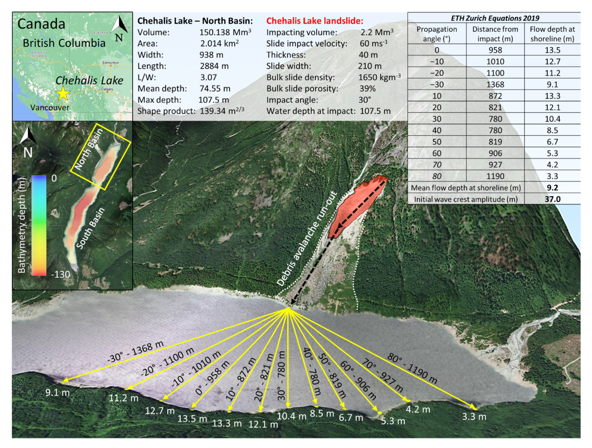
6. Example of Application of the Proposed Approach—The Chehalis Lake Landslide-Generated Wave

The landslide-induced wave in Chehalis Lake on 4 December 2007 (Figure 10, see Section 1) [6,7] is chosen as a test case of the proposed methodology for several reasons. It involves a representative mountain basin, and both the landslide [6] and lake characteristics [7] are well documented. In addition, multiple numerical modeling studies [6,42,43,44] provide insights into open-water hydrodynamics necessary to reproduce documented impacts. Bathymetric data acquired through a SONAR survey [7] are used in QGIS v3.16 to estimate the lake´s characteristics (see Section 2). The volume of the initial rockslide is estimated to be about 3 Mm³. The rock mass rapidly fragmented, transforming into a rock avalanche as it approached the shoreline. Approximately 2.2 Mm³ of rock debris entered the lake and triggered the wave [6,7,44]. Although this volume is larger than the one employed in hydrodynamics models (see Section 4), the maximum impact speeds are similar (about 60 ms⁻¹ [42,45], Figure 10), making the case study suitable for testing the method.

The case study data are first used as inputs in the empirical equations provided by Evers 2019 [46] (ETH-Zurich, 3D approach—Overland flow) to estimate flow depths at the Chehalis Lake shoreline. As this approach cannot be applied to the entire area of the lake, and because the lake is also divided into two sub-basins by a shallow subaqueous ridge, the test is limited to the north sub-basin (yellow rectangle in Figure 10). The sub-basins characteristics and landslide properties are summarized in Figure 10.

Flow depths are calculated at shoreline locations corresponding to wave propagation angles in 10° increments and ranging from −30° to +80° on both sides of the landslide midline (Figure 10). Calculations yield an open-water amplitude of the initial impulse wave of 37 m a.l.l., and shoreline flow depths ranging from 3.3 to 13.5 m, with a maximum opposite the slide source and a mean shoreline flow depth of 9.2 m (Figure 10).

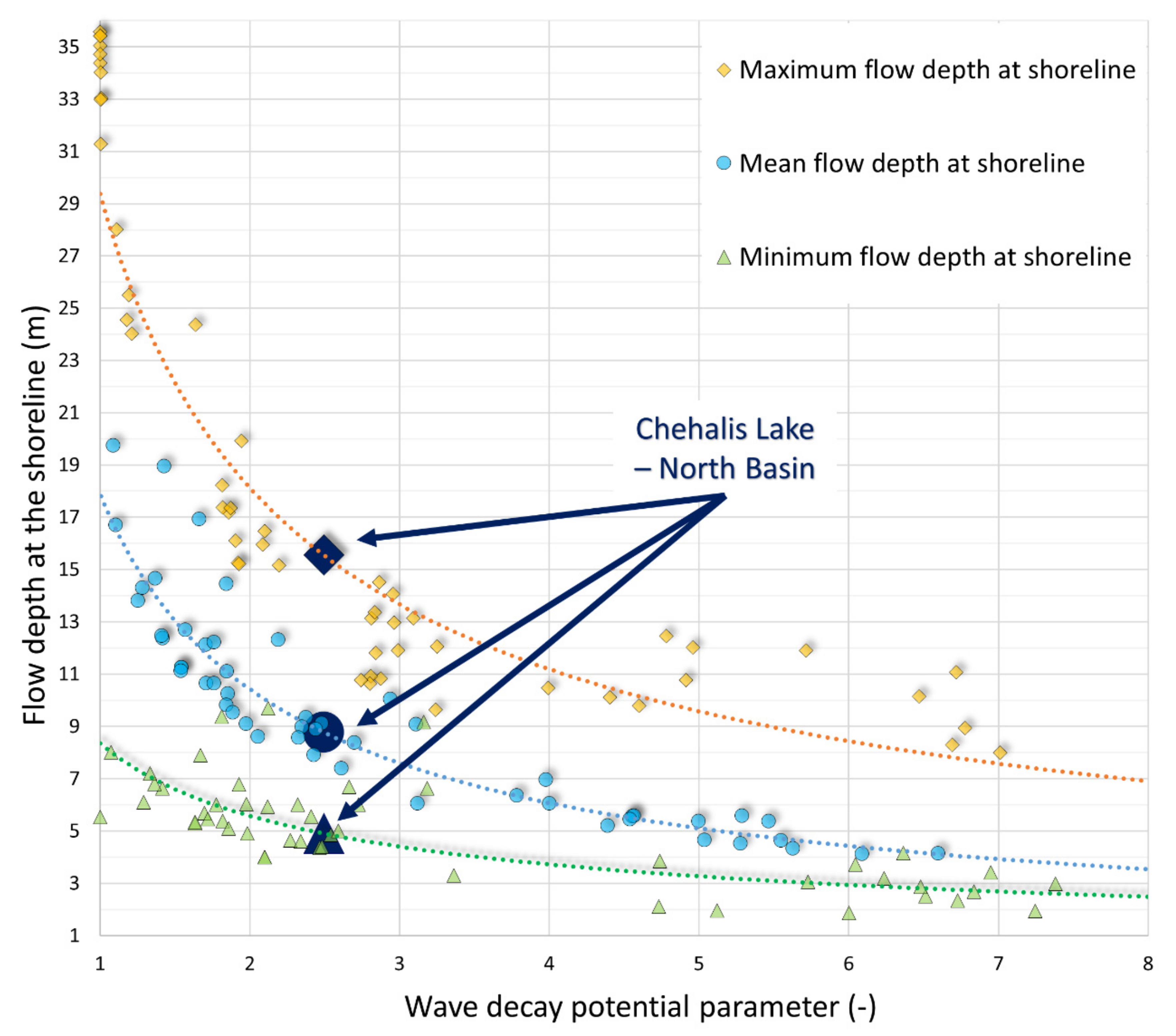
A ShpP value of 139.34 m^2/3 and a WDPP value of 2.495 (Equation (5) in Table 2 and Figure 8a) are calculated for the north sub-basin. Appling the latter value in Equations (6)–(8) yields estimates of maximum, mean, and minimum flow depths of 15.5, 8.8, and 4.9 m, respectively. The maximum and minimum values obtained with Equations (6)–(8) are higher than the ones obtained with the ETH equations, but a close match is found for the mean flow depth (Figure 9). However, the ratio of the maximum wave amplitude (37 m a.l.l.) and the WDPP of 2.49 is 14.8 m, which is very close to the maximum flow depth calculated using the ETH equations. These results pertain only to the north sub-basin of the Chehalis Lake. Considering the whole lake, the ShpP-value is 196 m^2/3 and the WDPP value is 3.36, yielding a slightly lower estimate of maximum, mean, and minimum flow depths at the shoreline of 12.63, 6.95, and 4.12 m, respectively.

These results show the applicability of the proposed method and use of equations in Table 3, with specific values of WDPP, for a preliminary evaluation of potential landslide-induced waves in natural alpine lakes to provide reliable estimates of the flow depths at the lake shoreline. Comparisons between the resulting flow depths obtained with the proposed equations and the ones derived using the ETH equations suggest that the new methodology provides a reliable estimate of flow characteristics. Regardless of what was observed with the presented test, appropriate validation of the proposed method is still required, where a comparison with real data or observations would increase the reliability of this approach’s application.

7. Comparison between Real and Theoretical Lakes

Based on this work, the WDPP is proposed as a suitable first-order descriptor of a lake basin’s potential for dissipating an impulse wave. Figure 11 is a plot of WDPP values superposed on the alpine lake classification. It provides a screening tool to identify lakes that are most likely to disperse a wave (Section 3). For the medium-size lakes, WDPP generally increases as lake size increases and depth decreases. This is consistent with the numerical modeling results (Figure 5)—lower water depths and longer distances to shorelines enhance wave dissipation and thus decrease shoreline flow depths.

In the case of large-size lakes, WDPP provides no clear separation of geometrical characteristics of lake basins (lake extent or depth), although a larger WDPP appears to be favored by larger lake volumes.

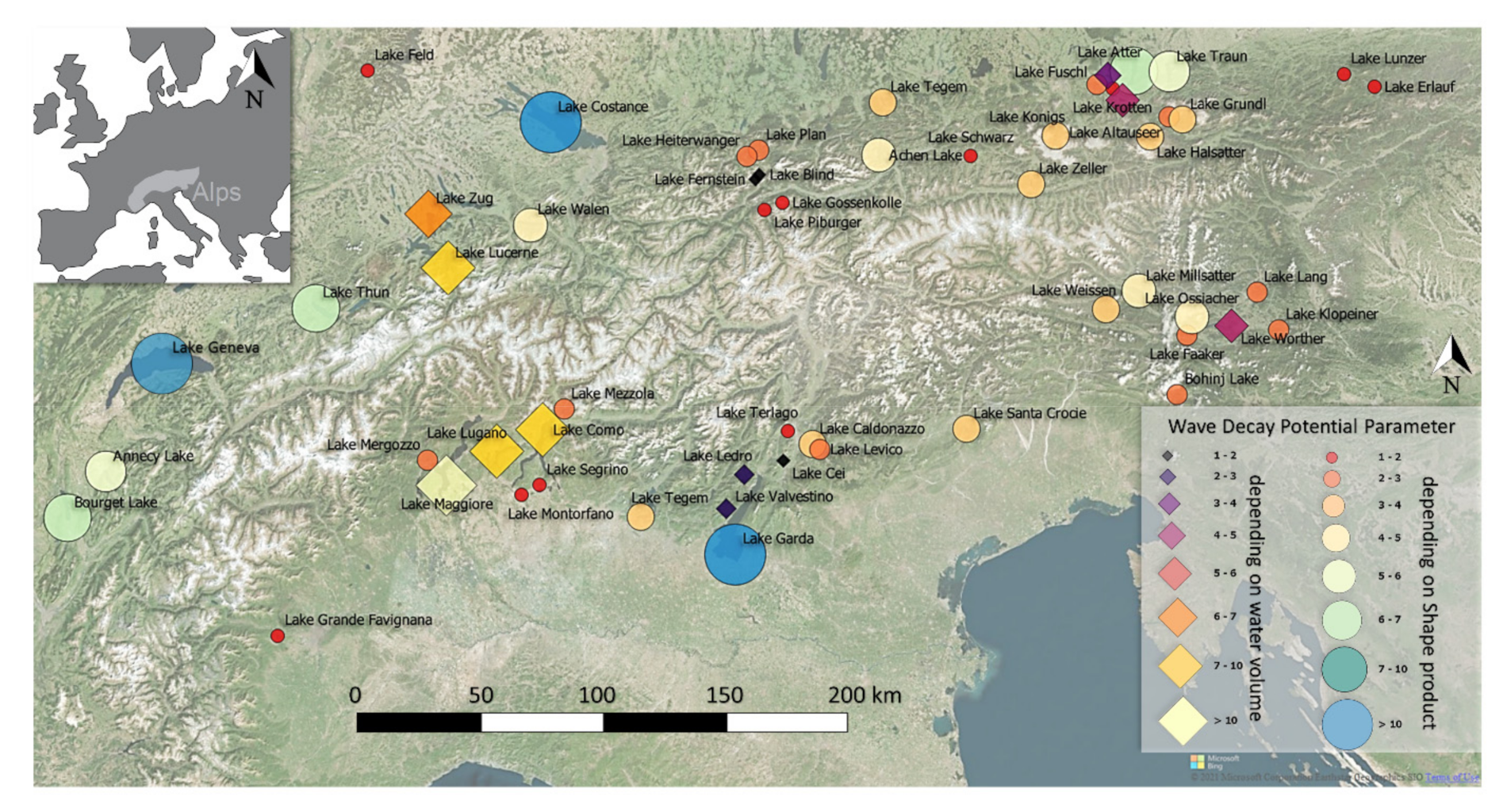
Figure 12 shows expected WDPP values for all the natural lakes in the Alps examined in this study. Circles on the map are lakes for which WDPP has been derived from ShpP Equation (5). Still, WDPPs for lakes with complex shapes (diamonds in Figure 12), for which ShpP is not available, are here based, for instance, on the water volume (Table 2, Equation (4)). Generally, high values of WDPP are related to perialpine lakes with large areas and volumes, whereas lower WDPP values are associated with smaller alpine lakes.

A critical issue in this work is the reliable range of lakes for which the new approach is applicable (see Table 1 and the complete table of theoretical lakes in the Supplementary Data). The data suggest that the approach has limitations when used for some lakes that are outside of this range, notably some large-size and very large-size lakes (i.e., WDPP > 7 in Figure 12). Further study is required to extend these investigations to alpine lakes outside of the stated range in this work to test the broader application of the proposed method.

8. Discussion and Further Required Research

8.1. Applicability of the Proposed Approach

The approach introduced in this work is intended to be a high-level screening tool for identifying the greatest landslide impulse wave threats and thus helping prioritize resources for a more detailed and thorough analysis. The study is based on 3D hydrodynamic modeling and considers a wide range of water body geometries. Results demonstrate the reliability of a lake geometry-based approach for a first-order assessment of the danger posed by potential landslide-triggered impulse waves in mountain lakes. The suggested method finds its applicability in situations where the characteristics of the possible impacting volume are unknown, as only the geometrical properties of lakes are required. Unlike other methods, this approach does not require a deep knowledge of wave theory or the need for additional software. A reliable constraint on wave attenuation, as is provided by this approach, means that the initial wave amplitude needs only to be generally approximated.

The method can be applied to lakes with diverse shapes and dimensions, subject to the limitation that the potential impacting volume has similar characteristics to the one adopted for the modeling in this work (Section 4). In the case of lakes with complex shapes, Equation (5) can be applied to sub-basins with specific geometrical properties to estimate the wave decay potential parameter WDPP, as has been done with the Chehalis Lake test case (Section 6). If Equation (5) is not applicable due to unknown lake-geometry parameters in Equation (2), WDPP can be estimated using Equation (3) or Equation (4), which consider lake area or volume respectively. The equations in Table 3 provide flow depths expected at the shoreline. However, because models with a maximum depth of less than 20 m were excluded from the later stages of the workflow, this method might overestimate the hazard potential for small shallow lakes.

The Chehalis Lake example shows that analyzing singular sub-basins provides a more conservative estimate of flow characteristics compared to an analysis of the entire lake. As waves propagating from one basin to the next may have already attenuated, sub-basin-specific estimations using this approach can be deemed as worst-case scenarios. It is worth noting that the subdivision of sub-basins does not take into account wave propagation from one basin to another. However, this limitation is a minor issue because a wave entering a second sub-basin has already significantly attenuated, implying that the highest threat is already identified by intra-basin events.

Nonetheless, wherever sub-basins join, complex variations in flow depth at the shoreline might be expected as impulse waves approach from the adjacent sub-basin. This is due to changes in bathymetry (e.g., a shallow sill as at Chehalis Lake, Figure 10), basin alignment (e.g., non-parallel valleys such as the western part of Lake Lucerne, Figure 1b), or both (e.g., the eastern part of Lake Lucerne, Figure 1b). In some instances, these effects might result in locally increased near-shore wave energy and run-up. As a consequence, although intra-basin wave generation gives a conservative assessment of near-shore wave threats, intra-basin waves may underestimate such threats where sub-basins join.

Given the numerical modeling results for the theoretical lakes (Section 5.1) and the results produced for the Chehalis Lake test (Section 6), it is concluded that the proposed approach is applicable for lakes that are flanked by steep unstable slopes, for which failures with volumes ranging from thousands to a few million cubic meters can be expected. However, this assertion requires validation with additional historical case studies from a variety of mountain regions, as well as fiords with basin characteristics similar to alpine lakes. Extending the dataset to other mountain regions for which good data are available (e.g., Canadian Cordillera or a select part of the Andes) to newly formed glacial water bodies [39] and artificial reservoirs would also improve the analysis and results.

8.2. Limitations, Uncertainties, and Further Potential Development

This work provides a workflow to estimate near-shore impulse-wave magnitude in terms of flow depth at the shoreline (see “Excel spreadsheet—Computational tool” in the Supplementary Materials). By contrast, most other studies report impacts in terms of inundation distance and run-up height, metrics that are not considered in this work. Nonetheless, shoreline water depth provides a preliminary characterization of run-up potential and inundation, although these are also heavily affected by the morphology and the steepness of the surrounding topography. As a result, observations of an impulse wave or post-event measurements of its impacts provide only a very general indication of the large-scale variability of flow depth at the shoreline. A more reasonable assessment of this new approach can be achieved using previously established relationships that independently estimate flow depth at the shoreline, as was done for the Chehalis Lake case study (Section 6).

A current disadvantage of this work is the lack of adequate validation. The Chehalis Lake case study and comparison of the results with those based on the ETH equations are insufficient to fully evaluate the validity of this approach. Proper validation would entail a comparison of the results derived using this method with real data collected in the field. However, flow depths at the shoreline caused by an impulse wave are not directly observable in the field and therefore must be calculated independently. Such calculation requires the use of detailed, site-specific, retrospective numerical simulations capable of accurately recreating a landslide-generated wave event.

Future extension and expansion of the proposed approach will involve two critical steps: (1) implementing numerical analyses on well documented, real-world events to validate the geometry-based strategy as a predictor of flow depth at the shoreline; and (2) developing rapid, low-computational-cost methods for estimating run-up and flooding potential from flow depth at the shoreline. This next phase of development will expand the range of outputs to include expected run-up, thereby extending the applicability of the proposed approach and enchaining opportunities to reliably validate it.

Another possible limitation of this study is its applicability to large lakes and a single impact volume. The size and properties of the impacting landslide substantially influence wave characteristics. For example, the maximum wave height resulting from an impact is dependent on landslide volume and competence, debris thickness and frontal width, impact speed, and slope angle and roughness [17,37]. Further research that addresses these issues is required. For example, the approach can be extended to consider diverse characteristics of the impacting volume to provide a relation for WDPP that considers landslide properties in addition to the geometrical characteristics of the lake (the ShpP). Incorporation of additional consideration into the workflow—including by varying impact processes, volumes, and velocities—might lead to the development of additional equations that can be applied to the full range of real-world situations. This can be accomplished in Flow-3D by adopting the concept of the impacting volume being a dense fluid, as done in the present study. Different volumes, shapes, impact velocities, and slope angles can be implemented in the model set-up. Scaling impact volumes relative to lake volume may assist in standardizing comparisons between lakes. In this work, the slide source is located halfway along the long side of the lake. Further development of the approach should consider different impacting locations along the lakeshore to extend the applicability of the suggested method. Moreover, it would be valuable to consider submerged slide sources, as subaqueous mass movements can also trigger lake impulse waves [47,48].

Further development of this methodology would also benefit from the inclusion of geotechnical properties of the materials that collapse and enter the lake. This would be especially interesting when studying mass movements made up of unlithified materials or heterogeneous rock masses, as well as studies of moraine-dammed lakes where large sediment masses can fail. Finally, landslide hazard and the erosional vulnerability of nearshore elements should be addressed in the context of risk analysis to complement the relative level of threat posed by the degree and pattern of impulse wave attenuation in a given basin.

9. Conclusions

A novel method for conducting a preliminary evaluation of the size and propagation of landslide-induced waves in mountain lakes is proposed. A set of equations is used within a numerical modeling framework to characterize the geometric characteristics of a lake and quickly assess the possible wave threat in terms of wave dissipation and expected flow depth along the shoreline (which is different from the expected run-up). Wave propagation controlled by lake geometry provides a general indication of where run-up or inundation would be the highest, although the behavior of the breaking wave is also heavily influenced by topography along the shoreline. The incorporation of landslide properties, behavior, and locations into the workflow will further increase the utility of this approach. The proposed method can be used as a first-order indicator for prioritizing lakes that appear to be particularly susceptible to landslide-induced impulse waves.

The findings of this study reveal that WDPP is a valid metric for the “dissipation power” (attenuation) of an impulse wave in a mountain lake and that it correlates well to lake geometrical characteristics, particularly area and water volume. The linear relationship between WDPP and ShpP, a metric that takes into account diverse lake properties, provides a valuable approach for estimating potential wave dissipation. If the ShpP is unavailable, for example in lakes with complex shapes, water volume can be used to estimate WDPP. Furthermore, WDPP can be used to calculate the expected flow depth at the lake shoreline. Results suggest that large perialpine lakes (V_w > 10.000 Mm³) are more likely to disperse impulse waves; these attenuate less in smaller alpine lakes (V_w < 10 Mm³).

This method can be applied worldwide to mountain lakes that differ in shape, extent, and volume. The minimum required input data are the geometrical characteristics of the lakes. Unlike other proposed methodologies, specific technical knowledge or additional inputs such as digital elevation data are not required, making the proposed method easy to use. However, inclusion of high-resolution digital bathymetric data would produce more accurate assessments.

The proposed method is tested with data available for the 2007 Chehalis Lake landslide-generated wave event. Results match well those obtained using the empirical equations published by ETH Zurich (2019 Edition—3D approach, [17,46]). Despite the positive results, one case study is insufficient to assess the overall reliability of our novel approach, and a validation considering real, observed data is still required. Indeed, additional historic events in which wave characteristics have been directly observed would be particularly valuable for further assessing the method. Furthermore, the applicability of impact volumes that differ from the one used in this study, together with a variety of impact characteristics, must be determined.

This study is an initial step in the development of this methodology; additional research is required to improve the method and its application, for example by taking into account properties of the potential impacting mass. Stability analyses of slopes bordering lakes with high hazards from impulse waves, including implications of external triggers such as intense rain events or earthquakes, are recommended to contribute to a proper estimate of the related hazard in a cascade effect context. Recently formed alpine lakes due to glacier retreat should also be included in these investigations.