Online SoC Estimation of Lithium-Ion Batteries Using a New Sigma Points Kalman Filter

Abstract

The accurate state of charge (SoC) online estimation for lithium-ion batteries is a primary concern for predicting the remaining range in electric vehicles. The Sigma points Kalman Filter is an emerging SoC filtering technology. Firstly, the charge and discharge tests of the battery were carried out using the interval static method to obtain the accurate calibration of the SoC-OCV (open circuit voltage) relationship curve. Secondly, the recursive least squares method (RLS) was combined with the dynamic stress test (DST) to identify the parameters of the second-order equivalent circuit model (ECM) and establish a non-linear state-space model of the lithium-ion battery. Thirdly, based on proportional correction sampling and symmetric sampling Sigma points, an SoC estimation method combining unscented transformation and Stirling interpolation center difference was designed. Finally, a semi-physical simulation platform was built. The Federal Urban Driving Schedule and US06 Highway Driving Schedule operating conditions were used to verify the effectiveness of the proposed estimation method in the presence of initial SoC errors and compare with the EKF (extended Kalman filter), UKF (unscented Kalman filter) and CDKF (central difference Kalman filter) algorithms. The results showed that the new algorithm could ensure an SoC error within 2% under the two working conditions and quickly converge to the reference value when the initial SoC value was inaccurate, effectively improving the initial error correction ability.

1. Introduction

With the rapid development of industry, the world today is facing many challenges, such as global warming, energy crisis and environmental degradation. As a new form of transportation, electric vehicles (EVs) have quickly become the focus of research and development in various automobile companies and research institutions due to their superior energy efficiency, braking energy recovery and low emissions [1,2,3]. The battery management system (BMS) is an integral component of EVs. It is used to monitor and manage battery packs to ensure the safety of EVs. The BMS can reasonably control the charge and discharge of the battery packs to increase the driving range, extend the battery life and reduce the vehicle operating cost [4,5,6,7]. Effective battery state of charge analysis, energy control management, battery fault diagnosis and safety are aspects of BMS technology that require improvement and continue to restrict the development of EVs. The accurate online estimation of the SoC of lithium-ion batteries is related to the ability to accurately predict the remaining range of an EV. Therefore, accurate online estimation of SoC is the key aspect of BMS technology [8,9].

At present, SoC estimation methods mainly include OCV-based estimation, ampere-hour integration estimation, internal resistance-based estimation, electrochemical model-based estimation, machine learning-based estimation, equivalent circuit-based estimation and modern control theory-based estimation. OCV is the stable electrode potential difference in the open-circuit state. In theory, the SoC-OCV relationship curves of the same batch of lithium-ion batteries are identical. However, as the battery cycle life [10,11,12] or the ambient temperature [13,14] changes, the SoC-OCV relationship curve changes accordingly. If the SoC-OCV curve cannot be obtained in a standardized and accurate manner, it is still a problem to use this method for SoC estimation. An adaptive method is established for the online estimation of OCV [15]. It needs to stand for a long time when measuring the battery OCV when the current excitation is a dynamic working condition; thus, the method based on OCV cannot accurately estimate the SoC. The ampere-hour integration method offers simple and reliable estimation, given that the initial SoC value and the current measurement value are accurate. Truchot et al. [16] used the ampere-hour integration method for strings cells online SoC estimation. Tang et al. improved SoC estimation accuracy by regularly calibrating battery capacity and SoC initial value. The SoC value estimated by the ampere-hour integration method without calibration was not found to be accurate [17]. The internal resistance of the battery represents the voltage response characteristics of the battery under current excitation. The internal resistance is equal to the ratio of the battery voltage change to the current change in a short period of time. Internal resistance is significantly affected by battery cycle life [18] and external temperature [19]. The mapping relationship between the internal resistance and SoC is not as reliable as the SoC-OCV curve, and online electrical impedance spectroscopy (EIS) measurements can be challenging [20]. Thus, SoC estimation based on the battery internal resistance is also challenging. Doyle et al. [21,22] established a pseudo-two-dimensional (P2D), electrochemical model based on the porous electrode and concentrated solution theories. The model includes a series of algebraic equations and partial differential equations, which can more accurately describe the lithium-ion diffusion and migration inside a battery. Additionally, the electrochemical reactions on the particle surface offer a detailed description of the microscopic reactions inside the battery. In the model established by Ahmed et al. [23], it is inconvenient to obtain material characteristic parameters such as the conductivity and diffusion coefficient. However, in this model there are more model parameters, and their identification is difficult, which makes the electrochemical model too difficult for online SoC estimation.

In recent years, artificial intelligence has received more and more attention. Machine learning is an important method to realize artificial intelligence. The machine learning method is applied to the field of battery technology. The machine learning method is based on battery measurement and operating data and realizes battery SoC estimation through algorithms such as neural networks. Wei et al. [24,25] combined neural networks and the Kalman filter for SoC estimation. Taimoor et al. [26] applied the adaptive fuzzy neural network to estimate the battery SoC and used 10 driving conditions to analyze and evaluate the proposed algorithm. Tong et al. [27] divided the battery working modes into three states, i.e., idle, charging and discharging. Three neural network models have been designed for battery SoC estimation. However, this method of preprocessing the battery load current can lead to some difficulties in estimating the SoC in real-time. In addition, the SoC estimation accuracy was affected by the state of health (SoH) [28]. Bian et al. [29] proposed a fusion-type SoH estimation method by combining model and data-based to enhance the SoC estimation accuracy and robustness. The main challenge of the machine learning method is obtaining a variety of data of actual working conditions of EVs for training. The machine learning method has high requirements on the processing capacity of automotive chips, which limits its practical application.

Significant efforts have been made to study novel methods that can balance the model complexity and calculation efficiency. The equivalent circuit model (ECM) is an ideal candidate. The ECM uses circuit components such as resistors, capacitors and voltage sources to reflect the electrochemical characteristics of the battery. The voltage source in the model represents the thermodynamic equilibrium potential of the battery, and the resistance and capacitance represent the dynamic characteristics of the battery. Zhang et al. [30] used a first-order hysteresis model, and Liu et al. [31] used a fractional-order model to further improve the accuracy of the terminal voltage simulation of the battery. The battery SoC estimation method based on the ECM can better balance the model complexity and calculation efficiency [32]. Bian et al. [33] optimized the parameters of ECM through the particle swarm optimization algorithm, which effectively improved the estimation accuracy of SoC. In order to further reduce the influence of process noise on the model and improve SoC estimation accuracy, modern control theory has been applied to SoC estimation. The Kalman filter family algorithms solve the filter gain, covariance and SoC estimation value by comparing the measured voltage and the model voltage. Li et al. [34] used the Extended Kalman filter (EKF) method for SoC estimation. The extended Kalman filter locally linearizes the non-linear state function and measurement function of the battery through the first-order Taylor series expansion and then performs the Kalman filter. Thus, it is a sub-optimal filter. EKF needs to calculate the Jacobian matrix of the non-linear function and requires the state function and the measurement function to be continuously differentiable. For Gaussian systems, the Jacobian matrix solution process is cumbersome and easily leads to poor numerical stability of EKF and even calculation divergence.

In order to overcome these problems, Plett explored a new technique called the Sigma Point Kalman Filter (SPKF) [35,36], which uses approximate conditional probability density functions instead of non-linear models. The results showed that SPKF is better than EKF in terms of battery SoC estimation accuracy and error range. Schei et al. [37] first proposed the use of central difference to improve the EKF algorithm. Unlike research in unscented Kalman filter (UKF) filtering theory, Ito et al. [38] proposed central difference filtering (CDF) based on the Stirling interpolation formula. Norgaad et al. [39] first proposed divided difference filtering (DDF). Merwe et al. [40] unified these two essentially identical filters and collectively referred to it as the central differential Kalman filter (CDKF). The CDKF algorithm considers the statistical characteristics of Gaussian random variables and uses the prior distribution to construct a set of deterministic Sigma points. The Sigma points obtained after the linear regression transformation was used to represent the posterior distribution of the system state. The CDKF uses a simple interpolation formula to obtain the approximation form of the function. It does not require the calculation of the derivative of the function or the Jacobian matrix of the non-linear function, which can significantly reduce the number of calculations required. The UKF replaces the local linearization in the EKF with an unscented transform. UKF also does not need to calculate the Jacobian matrix, and in theory, the unscented transformation can at least approximate the posterior mean and covariance of any non-linear Gaussian system state with third-order Taylor accuracy.

Unlike previous research, this study involves an effective combination of unscented transformation and Stirling interpolation center difference algorithm for online SoC estimation of lithium-ion batteries. The new algorithm constructs different Sigma points sets through proportional correction sampling and symmetric sampling and performs battery SoC estimation twice. The new algorithm overcomes the shortcomings of the original CDKF algorithm, such as weak initial error correction ability and large end error when the initial SoC value is inaccurate, ensuring efficient calculation. The proposed algorithm was compared with EKF, CDKF and UKF. Through different initial SoC guess values and different dynamic conditions, the initial error correction capability and error range of each algorithm was analyzed. Five error analysis indicators and initial error correction time were used to verify the error range and effectiveness of the new algorithm. Specifically, the SoC-OCV curve was accurately obtained by the interval static method in Section 2.1, and the parameter identification of the equivalent circuit model was performed using the DST operating conditions in Section 2.2. Section 3 describes the design process of the proposed algorithm. In Section 4, a semi-physical simulation platform based on dSPACE Rapid Prototyping Systems is constructed, and the proposed algorithm is verified under two working conditions, i.e., US06 Highway Driving Schedule (US06) and Federal Urban Driving Schedule (FUDS).

2. Modeling and Parameter Identification

2.1. Acquisition of SoC-OCV Curve

The battery used in the test is a 18,650 cell and the basic parameters of the battery are shown in

Table 1. Specifications of battery samples.

Type	Capacity Rating	Nominal Voltage	Upper Cut-Off Voltage	Lower Cut-Off Voltage
18,650	2000 mA h	3.6 V	4.2 V	2.5 V

.

The accurate calibration of the SoC-OCV relationship curve is the first step to accurately estimating the SoC. It is mentioned in more literature that the interval static method as the most suitable way to obtain the SoC-OCV curve. The instruments involved in this study to obtain the SoC-OCV mapping relationship mainly include the Arbin BT2000 Battery Test System and Temperature Chamber.

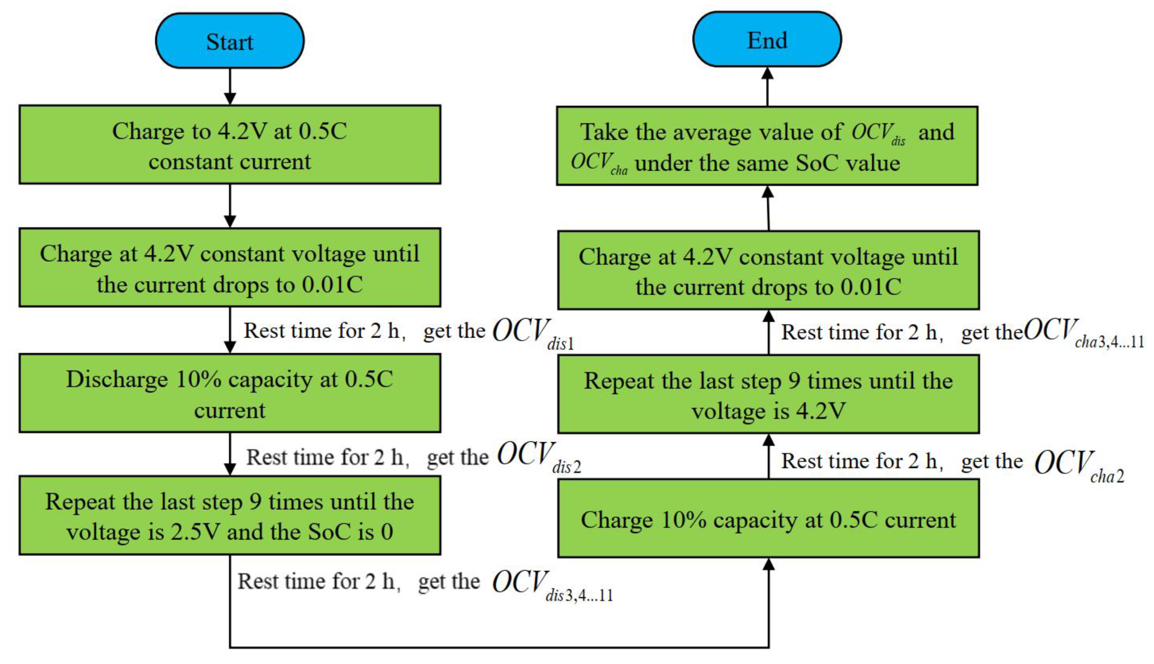
The charge and discharge tests of the battery were carried out by the interval static method at a temperature of 25 °C. The steps are shown in Figure 1.

We obtained a total of 11 sets of data for each of OCV_cha and OCV_dis. After taking the average of OCV_cha and OCV_dis under the same SoC value, the results are shown in

Table 2. Data points of SoC-OCV.

Number	1	2	3	4	5	6	7	8	9	10	11
OCV(V)	3.297	3.479	3.571	3.606	3.634	3.675	3.765	3.854	3.954	4.064	4.180
SoC	0.0005	0.1	0.2	0.3	0.4	0.5	0.6	0.7	0.8	0.9	1

.

The SSE refers to the sum of squares due to error. This statistical parameter calculates the sum of the squares of the error between the fitted data and the corresponding points of the original data. The closer the SSE value is to 0, the better is the model selection and fitting, leading to successful prediction capabilities.

$$SSE={\displaystyle \sum _{i=1}^n}{\omega }_i{(y_i-\stackrel{\wedge }{y_i})}^2$$

(1)

where, ω_i is the weight, y_i is the actual value and $\stackrel{\wedge }{y_i}$ is the predictive value.

The adjusted R-square refers to the coefficient of determination, which is between 0 and 1 for this equation. The closer the coefficient is to 1, the stronger the explanatory power of the variables of the equation is for y, and the model fits the data more accurately.

The RMSE refers to the root mean square error, also called the standard deviation of the regression system. The closer its value is to 0, the better is the model selection and fitting, and the more successful is the data prediction.

$$RMSE=\sqrt{\frac{1}{n}{\displaystyle \sum _{i=1}^n}{\omega }_i{(y_i-\stackrel{\wedge }{y_i})}^2}$$

(2)

In this work, three indicators of SSE adjusted R-square and RMSE were used to compare the fit of the SoC-OCV mapping curve at different orders, as shown in

Table 3. Comparison of the goodness of fit of the SoC-OCV curve.

Fitting Order	SSE	Adjusted R-Square	RMSE
4	0.0007965	0.9981	0.01152
5	0.0002463	0.9993	0.007019
6	0.0001321	0.9995	0.005746
7	0.00007738	0.9996	0.005079
8	0.00005769	0.9996	0.005371
9	0.00005408	0.9992	0.007354

.

Table 3 indicates that when the fitting order is 7, the quality of fit is the best. The fitting formula of OCV related to SoC is as follows (Equation (3)) and the obtained SoC–OCV relationship curve is shown in Figure 2.

$$\begin{array}{l}{U}_{OCV}=-30.52\times So{C}^7+115.94\times So{C}^6-169.67\times So{C}^5+115.55\times So{C}^4\\ -31.71\times So{C}^3-0.85\times So{C}^2+2.13\times SoC+3.30\end{array}$$

(3)

2.2. The Second-Order RC Battery ECM

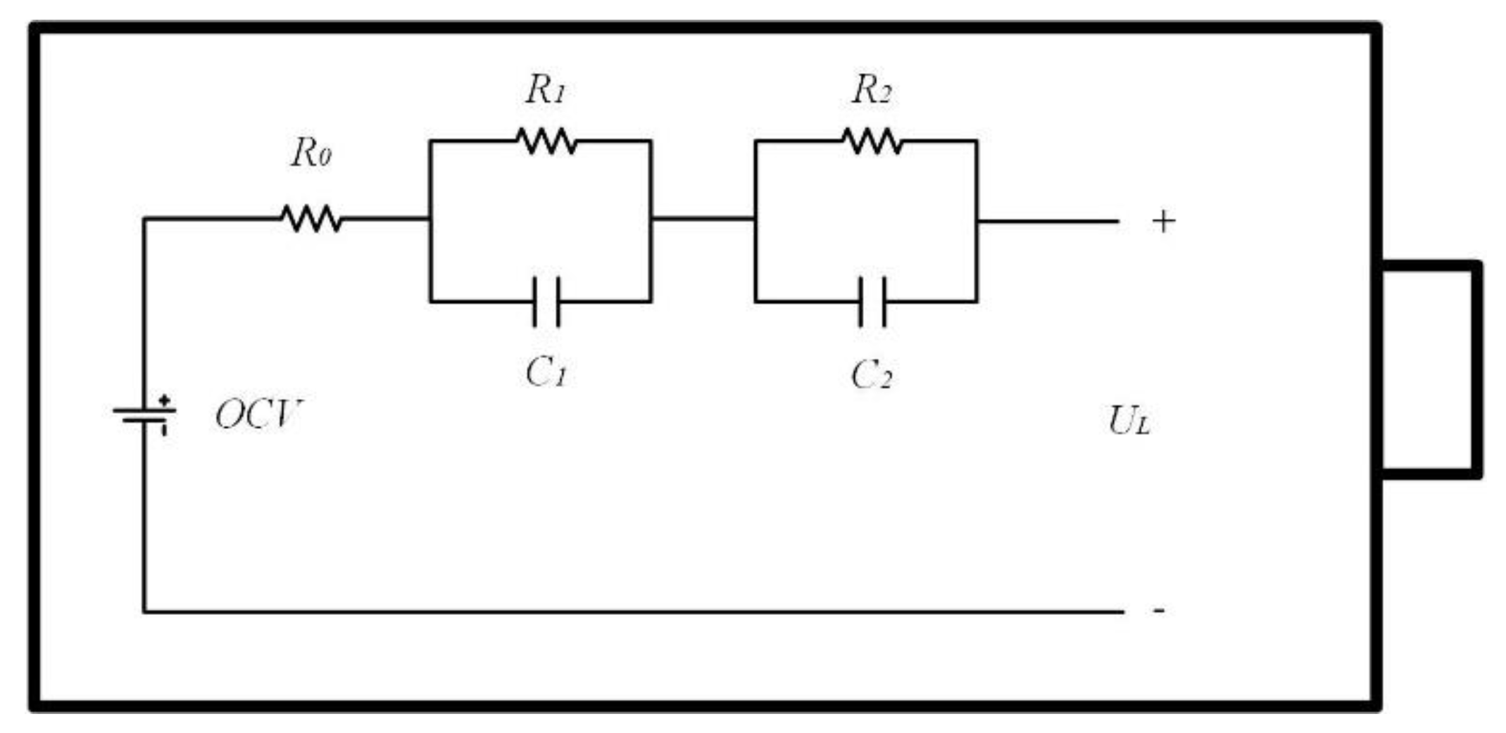
According to the working mechanism of the lithium-ion battery, a model of the second-order RC ECM (2-RC ECM) was established, as shown in Figure 3. The model mainly includes an ideal voltage source, i.e., the OCV of the battery, an ohmic internal resistance, R₀, and two RC networks. R₁ and R₂ are the polarization internal resistances, and C₁ and C₂ are polarization capacitors. Among them, the parallel circuit of R₁ and C₁ mainly simulate the short-time constant electrochemical polarization phenomenon in the electrode, and the parallel circuit of R₂ and C₂ mainly simulates the long-time constant concentration difference polarization phenomenon related to the diffusion process in the electrolyte and the porous electrode. The 2-RC ECM has a good balance between computational complexity and model accuracy. Therefore, we chose this model.

Based on the 2-RC ECM, the state equation (Equation (4)) and measurement equation (Equation (5)) could be obtained using the Kirchhoff voltage and current laws.

$$\{\begin{array}{l}{\dot{U}}_1=\frac{I_L}{C_1}-\frac{U_1}{R_1{C}_1}\\ {\dot{U}}_2=\frac{I_L}{C_2}-\frac{U_2}{R_2{C}_2}\end{array}$$

(4)

$$U_L=U_{OCV}-I_L{R}_0-U_1-U_2$$

(5)

According to the SoC definition and the ampere-hour integration method, the continuous-time state equation can be obtained.

$$SoC(t)=So{C}_0-\frac{\eta }{Q_N}{\int }_0^t{I}_L(t)dt$$

(6)

Due to the need of Kalman filter, Equation (4) was solved and discretized, Equation (6) was discretized. The discrete-time state space representation (Equation (7)) and measurement equation (Equation (8)) were established.

$$\left[\begin{array}{l}SoC(k+1)\\ U_1(k+1)\\ U_2(k+1)\end{array}\right]=\left(\begin{array}{ccc}1& 0& 0\\ 0& e^{-\frac{\Delta t}{{\tau }_1}}& 0\\ 0& 0& e^{-\frac{\Delta t}{{\tau }_2}}\end{array}\right)\times \left[\begin{array}{l}SoC(k)\\ U_1(k)\\ U_2(k)\end{array}\right]+\left[\begin{array}{c}-\frac{\eta \Delta t}{Q_N}\\ R_1(1-e^{-\frac{\Delta t}{{\tau }_1}})\\ R_2(1-e^{-\frac{\Delta t}{{\tau }_2}})\end{array}\right]\times I_L(k)+\omega (k)$$

(7)

$$U_L(k)=U_{OCV}(k)-I_L(k)\times R_0(k)-U_1(k)-U_2(k)+\nu (k)$$

(8)

The circuit parameters include open circuit voltage U_OCV, circuit current I_L, battery load terminal voltage U_L, internal resistance R₀, polarization internal resistances R₁ and R₂, polarization capacitance C₁ and C₂, the initial SoC SoC₀, coulombic efficiency η, the nominal capacity Q_N, the system state input error ω(k), the observation error ν(k), and time constants, τ₁ and τ₂, where, τ₁ = R₁ C₁ and τ₂ = R₂ C₂. U₁ is the voltage of R₁, and U₂ is the voltage of R₂.

2.3. Parameter Identification

According to the dynamic stress condition (DST) test rules mentioned in the “USABC Electric Vehicle Battery Test Manual”, the battery sample was charged and discharged. Based on the charge and discharge current and voltage data under the DST condition, the unknown parameters (R₀, R₁, R₂, C₁, C₂) in the state equation were identified using the recursive least square method. The parameter estimation matrix (Equation (9)), observation matrix (Equation (10)) and transfer function (Equation (12)) are as follows:

$$\theta (k)={\left[a_1,a_2,a_3,a_4,a_5\right]}^T$$

(9)

$$\phi (k)={\left[\Delta V(k-1),\Delta V(k-2),I(k),I(k-1),I(k-2)\right]}^T$$

(10)

where the differential voltage is given by

$$\Delta V(k)=U_{OCV}(k)-U_L(k)$$

(11)

$$G(s)=\frac{U_{OCV}(s)-U_L(s)}{I_L(s)}=\frac{R_0{s}^2+\frac{1}{{\tau }_1{\tau }_2}(R_0{\tau }_1+R_0{\tau }_2+R_2{\tau }_1+R_1{\tau }_2)s+\frac{R_0+R_1+R_2}{{\tau }_1{\tau }_2}}{s^2+\frac{({\tau }_1+{\tau }_2)}{{\tau }_1{\tau }_2}s+\frac{1}{{\tau }_1{\tau }_2}}$$

(12)

The parameter identification steps of the recursive least squares method with the forgetting factor are as follows:

$$K(k)=\frac{P(k-1)\phi (k)}{\phi {(k)}^{T}P(k-1)\phi (k)+\lambda }$$

(13)

$$\epsilon (k)=y(k)-\theta {(k)}^T\cdot \phi (k)$$

(14)

$$P(k)={\lambda }^{-1}(P(k-1)-K(k)\phi {(k)}^{T}P(k-1))$$

(15)

$$\theta (k)=\theta (k-1)+K(k)\epsilon (k)$$

(16)

where, K(k) is the RLS gain matrix, ε(k) is the output estimation error matrix, P(k) is the covariance matrix, φ(k) is the observation matrix, θ(k) is the parameter estimation matrix and λ is the forgetting factor.

The functional relationship between the five parameters (R₀, R₁, R₂, C₁, C₂) and $\theta (k)={\left[a_1,a_2,a_3,a_4,a_5\right]}^T$ is derived as follows.

$$R_0=\frac{a_3-a_4+a_5}{1+a_1-a_2}$$

(17)

$${\tau }_1\times {\tau }_2=\frac{T^2\times (1+a_1-a_2)}{4\times (1-a_1-a_2)}$$

(18)

$${\tau }_1+{\tau }_2=\frac{T\times (1+a_2)}{1-a_1-a_2}$$

(19)

$$R_0+R_1+R_2=\frac{a_3+a_4+a_5}{1-a_1-a_2}$$

(20)

$$R_0{\tau }_1+R_0{\tau }_2+R_2{\tau }_1+R_1{\tau }_2=\frac{T\times (a_3-a_5)}{1-a_1-a_2}$$

(21)

$T$ is the sampling time.

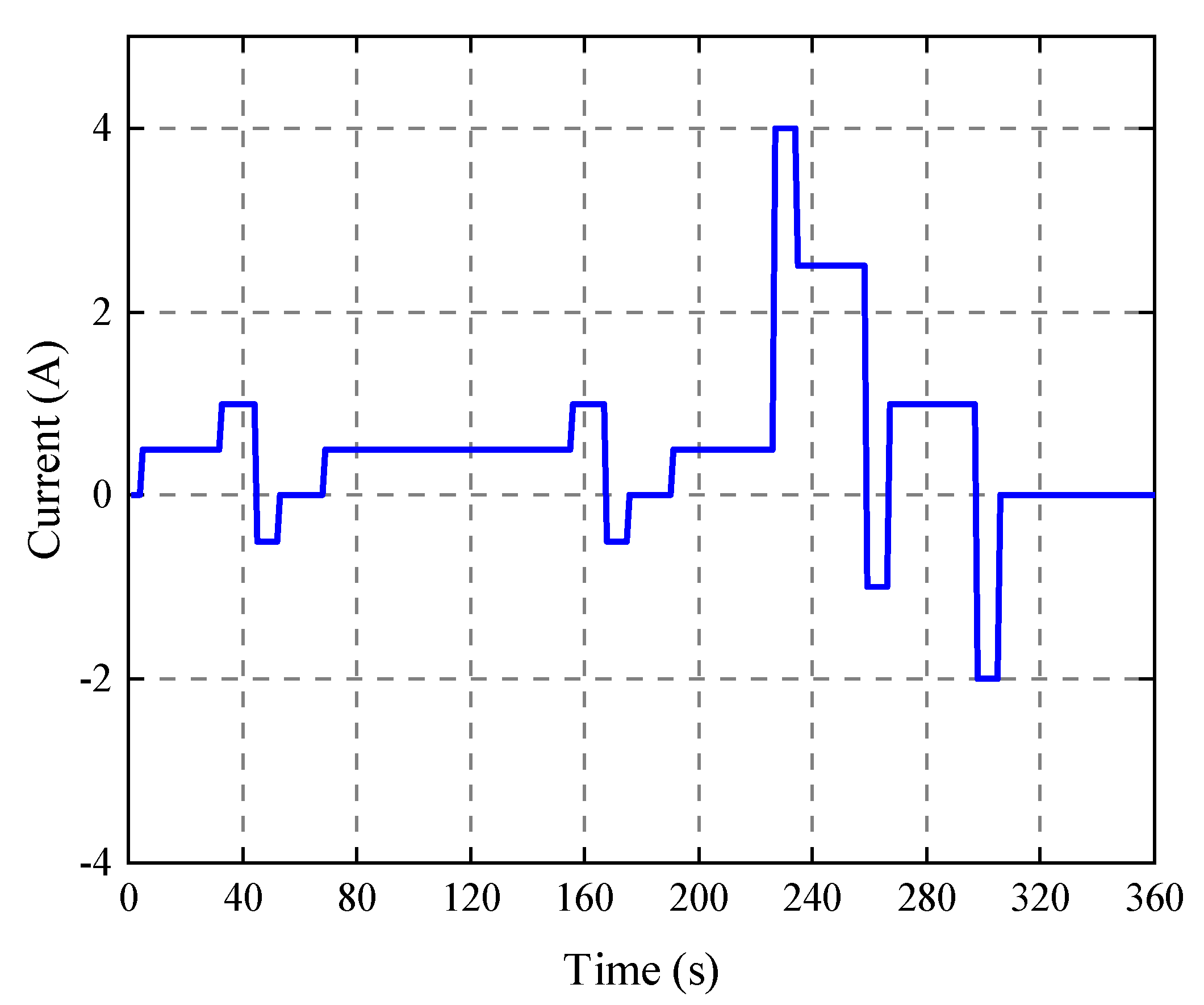
HPPC is a pulse constant current discharge condition. The HPPC condition is used to identify the parameters of the equivalent circuit model in the literature. The real operating conditions of EVs are much more complicated than HPPC, and the parameters identified by the HPPC operating condition may not be able to estimate the battery status under complex operating conditions well. In this paper, the DST operating condition is selected as the model parameter identification of dynamic battery behavior. A complete DST operating condition cycle is 360 s, as shown in Figure 4.

First, the discrete-time state-space representation (Equation (7)) and measurement equation (Equation (8)) were established. Then, based on the SoC-OCV mapping relationship curve, the equation parameter identification was carried out. The parameter identification results are shown in

Table 4. Parameter identification results of ECM.

R0 (Ω)	R1 (Ω)	C1 (F)	R2 (Ω)	C2 (F)
0.07009	0.002101	120.8	0.03927	1327.0

.

3. Proposed Algorithm Design and Flow

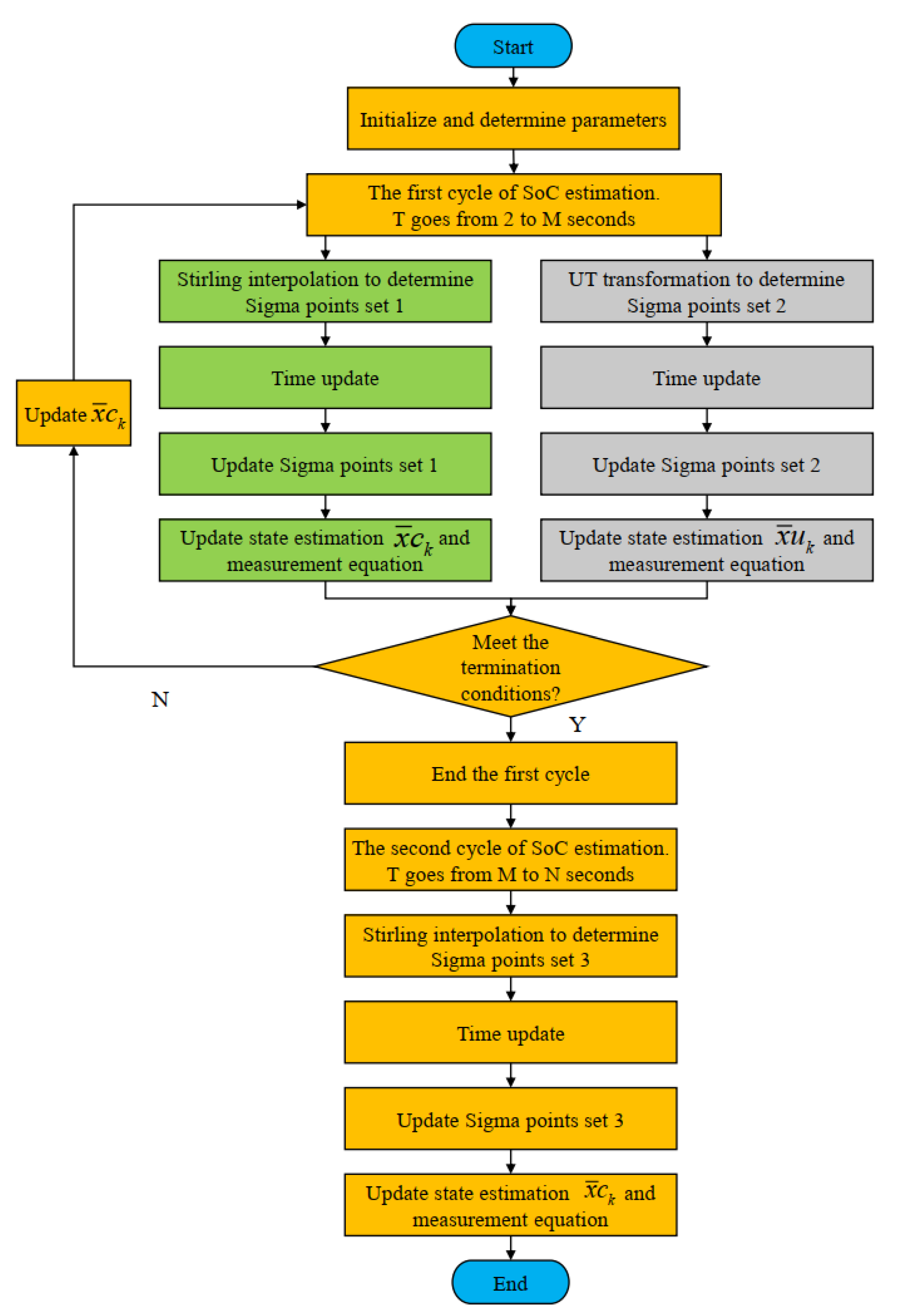
The new proposed algorithm is based on the Stirling interpolation, and UT transformation to determine Sigma points set 1 and Sigma points set 2 to start the first cycle, as shown in Figure 5. The two sets of the sampling points have the same mean and covariance as the system state distribution. After updating the time and measurement, the state estimation, $\overline{x}$c_k, was compared with $\overline{x}$u_k to update $\overline{x}$c_k. When the termination conditions were met, the algorithm entered the second cycle. Based on the Stirling interpolation, Sigma point set 3, were determined. Then, after the time and measurement update, the posterior mean and covariance of the system state were calculated.

The charge and discharge time of the battery under a certain working condition was set to N seconds.

S1: Initialization.

(1) The SoC-OCV relationship curve and the 2-RC ECM model parameters, R₀, R₁, R₂, C₁, and C₂, were prepared.

(2) The initial value of SoC was guessed and the initial covariance matrix P₀ at the first second was set.

(3) The noise, ω(k), and the measuring equation noise ν(k) were set.

(4) The given interval length of the central difference transform was set to h = 1.6, and the state vector dimension was set to L = 3.

S2: Determination of weight.

The weights, W_c1, W_m, and W_c, were calculated as follows:

$$W_{c1}=\frac{1}{4\times h^2}$$

(22)

$$W_m(1)=\frac{\lambda }{L+\lambda }$$

(23)

$$W_c(1)=\frac{1}{L+\lambda }+1-{\alpha }^2+\beta$$

(24)

When jj goes from 2 to 2L + 1,

$$W_m(jj)=\frac{1}{2\times (L+\lambda )}$$

(25)

$$W_c(jj)=\frac{1}{2\times (L+\lambda )}$$

(26)

And α = 0.01, β = 2, λ = 3 × α² − L.

S3: In the first cycle of SoC estimation, time t goes from 2 to M seconds.

(1) Determination of the Sigma points sets.

a. The Stirling interpolation was used to determine the Sigma points set 1.

$$\chi c_{k-1}=\left[\overline{\chi }{c}_{k-1},\overline{\chi }{c}_{k-1}+h\sqrt{P_{k-1}},\overline{\chi }{c}_{k-1}-h\sqrt{P_{k-1}}\right]$$

(27)

b. The UT transformation was used to determine the Sigma points set 2.

$$\chi u_{k-1}=\left[\overline{\chi }{u}_{k-1},\overline{\chi }{u}_{k-1}+\sqrt{(L+\lambda )P_{k-1}},\overline{\chi }{u}_{k-1}-\sqrt{(L+\lambda )P_{k-1}}\right]$$

(28)

(2) Time update and calculation of the prior mean and covariance.

The Cholesky decomposition of the covariance was performed.

$$P_{k-1}=S_{k-1}^x{(S_{k-1}^x)}^T$$

(29)

$$S_{k-1}^x=[S_{k-1}^{x,1}\cdots S_{k-1}^{x,n}]$$

(30)

$$\chi c^i{}_{k|k-1}=A\overline{\chi }{c}_{k-1}+Bu(t-1)$$

(31)

$$\begin{array}{l}P{c}_{k|k-1}={\displaystyle \sum _{i=1}^L{W}_{c1}(i)\left\{\left[A(\overline{\chi }{c}^i{}_{k|k-1}+h\sqrt{P_{k-1}})+Bu(t-1)\right]-\left[A(\overline{\chi }{c}^i{}_{k|k-1}-h\sqrt{P_{k-1}})+Bu(t-1)\right]\right\}}\\ {\left\{\left[A(\overline{\chi }{c}^i{}_{k|k-1}+h\sqrt{P_{k-1}})+Bu(t-1)\right]-\left[A(\overline{\chi }{c}^i{}_{k|k-1}-h\sqrt{P_{k-1}})+Bu(t-1)\right]\right\}}^T+{\displaystyle \sum \omega }\end{array}$$

(32)

$$\chi u^i{}_{k|k-1}=A\overline{\chi }{u}_{k-1}+Bu(t-1)$$

(33)

$$\overline{x}{u}_{k|k-1}=\chi u^i{}_{k|k-1}={\displaystyle \sum _{i=0}^{2L}{W}_m(i)}\chi u^i{}_{k|k-1}$$

(34)

$$P{u}_{k|k-1}={\displaystyle \sum _{i=0}^{2L}{W}_c(i)}\left[\chi u^i{}_{k|k-1}-\overline{x}{u}_{k|k-1}\right]{\left[\chi u^i{}_{k|k-1}-\overline{x}{u}_{k|k-1}\right]}^T+{\displaystyle \sum \omega }$$

(35)

where, $A=\left(\begin{array}{ccc}1& 0& 0\\ 0& e^{-\frac{\Delta t}{{\tau }_1}}& 0\\ 0& 0& e^{-\frac{\Delta t}{{\tau }_2}}\end{array}\right)$, $B=\left[\begin{array}{c}-\frac{\eta \Delta t}{Q_N}\\ R_1(1-e^{-\frac{\Delta t}{{\tau }_1}})\\ R_2(1-e^{-\frac{\Delta t}{{\tau }_2}})\end{array}\right]$, $u=I_L$.

(3) Updating the Sigma points sets.

a. Sigma points set 1 was updated.

$$\chi c_{k|k-1}=\left[\overline{\chi }{c}_{k|k-1},\overline{\chi }{c}_{k|k-1}+h\sqrt{P{c}_{k|k-1}},\overline{\chi }{c}_{k|k-1}-h\sqrt{P{c}_{k|k-1}}\right]$$

(36)

b. Sigma points set 2 was updated.

$$\chi u_{k|k-1}=\left[\overline{\chi }{u}_{k|k-1},\overline{\chi }{u}_{k|k-1}+\sqrt{(L+\lambda )P{u}_{k|k-1}},\overline{\chi }{u}_{k|k-1}-\sqrt{(L+\lambda )P{u}_{k|k-1}}\right]$$

(37)

(4) The measurement equation was updated.

a. The state estimation and measurement equation update based on the Sigma point set 1.

$$\overline{y}{c}_{k|k-1}=H(\overline{x}{c}_{k|k-1},r_k)$$

(38)

$$P{c}_{\overline{y}{c}_k}={\displaystyle \sum _{i=1}^L\left\{\begin{array}{l}{W}_{c1}(i)\left[(H_k(\overline{\chi }{c}_{k|k-1}+h\sqrt{P{c}_{k|k-1}})-H_k(\overline{\chi }{c}_{k|k-1}-h\sqrt{P{c}_{k|k-1}})\right]\\ {\left[(H_k(\overline{\chi }{c}_{k|k-1}+h\sqrt{P{c}_{k|k-1}})-H_k(\overline{\chi }{c}_{k|k-1}-h\sqrt{P{c}_{k|k-1}})\right]}^T\end{array}\right\}}+R_k$$

(39)

$$\begin{array}{l}P{c}_{\overline{x}{c}_k,\overline{y}{c}_k}={\displaystyle \sum _{i=1}^L\sqrt{W_{c1}(i)}}[(\overline{\chi }{c}_{k|k-1}+h\sqrt{P{c}_{k|k-1}})-\overline{\chi }{c}_{k|k-1}]\\ {\left[(h_k(\overline{\chi }{c}_{k|k-1}+h\sqrt{P{c}_{k|k-1}})-h_k(\overline{\chi }{c}_{k|k-1}-h\sqrt{P{c}_{k|k-1}})\right]}^T\end{array}$$

(40)

where, $H(k)=\left[\begin{array}{ccc}\frac{\partial U_{OCV}(k)}{\partial SoC(k)}-I_L(k)\times \frac{\partial R_0(k)}{\partial SoC(k)}& -1& -1\end{array}\right]$

Calculation of the Kalman gain:

$$K{c}_k=P{c}_{\overline{x}{c}_k,\overline{y}{c}_k}/P{c}_{\overline{y}{c}_k}$$

(41)

Status estimation update:

$$\overline{x}{c}_k=\overline{x}{c}_{k|k-1}+K{c}_k(y{c}_k-\overline{y}{c}_{k|k-1})$$

(42)

Covariance update:

$$P{c}_k=P{c}_{k|k-1}-K{c}_{k}P{c}_{\overline{y}{c}_k}K{c}_k{}^T$$

(43)

$$Xc(:,t)=\overline{x}{c}_k$$

(44)

b. State estimation and measurement equation update based on the Sigma points set 2.

$$\overline{y}{u}_{k|k-1}=H(\overline{x}{u}_{k|k-1},r_k)$$

(45)

$$P{u}_{\overline{y}{c}_k}={\displaystyle \sum _{i=0}^{2L}\left\{\begin{array}{l}{W}_c(i)\left[H_k(\overline{\chi }{u}_{k-1}+\sqrt{(L+\lambda )P{u}_{k-1}})-\overline{y}{u}_{k|k-1}\right]\\ {\left[(H_k(\overline{\chi }{u}_{k-1}+\sqrt{(L+\lambda )P{u}_{k-1}})-\overline{y}{u}_{k|k-1}\right]}^T\end{array}\right\}}+R_k$$

(46)

$$\begin{array}{l}P{u}_{\overline{x}{c}_k,\overline{y}{c}_k}={\displaystyle \sum _{i=0}^{2L}{W}_c(i)}[(\overline{\chi }{u}_{k-1}+\sqrt{(L+\lambda )P{u}_{k-1}})-\overline{\chi }{u}_{k|k-1}]\\ {\left[H_k(\overline{\chi }{u}_{k-1}+\sqrt{(L+\lambda )P{u}_{k-1}})-\overline{y}{u}_{k|k-1}\right]}^T\end{array}$$

(47)

Calculation of the Kalman gain:

$$K{u}_k=P{u}_{\overline{x}{c}_k,\overline{y}{c}_k}/P{u}_{\overline{y}{c}_k}$$

(48)

Status estimation update:

$$\overline{x}{u}_k=\overline{x}{u}_{k|k-1}+K{u}_k(y{u}_k-\overline{y}{u}_{k|k-1})$$

(49)

Covariance update:

$$P{u}_k=P{u}_{k|k-1}-K{u}_{k}P{u}_{\overline{y}{c}_k}K{u}_k{}^T$$

(50)

$$Xu(:,t)=\overline{x}{u}_k$$

(51)

(5) Determining whether the termination conditions are met and correcting the initial error of the SoC estimate.

Taking the first row of the two matrices, Xc(:, t) and Xu(:, t) at time t:

$$Xc(1,t),Xu(1,t)$$

(52)

$$\mathrm{If}\left|\frac{\left[Xc(1,t)-Xu(1,t)\right]}{Xu(1,t)}\right|>\delta$$

(53)

$$\mathrm{Then}Xc(:,t)=\overline{x}{u}_k$$

(54)

$$\mathrm{Else}\mathrm{If}\left|\frac{\left[Xc(1,t)-Xu(1,t)\right]}{Xu(1,t)}\right|\le \delta$$

(55)

Here, δ is the threshold value. Set δ to 0.0000015.

This circle was ended, and the time t was printed. Then, M = t.

S4: The second cycle, time t from M to N seconds.

(1) Determination of the Sigma points set 3.

Subject to (27)

(2) Time update and calculation of the prior mean and covariance.

$$\chi c^i{}_{k|k-1}=A\overline{\chi }{c}_{k-1}+Bu(k-1)$$

(56)

$$\begin{array}{l}P{c}_{k|k-1}={\displaystyle \sum _{i=1}^L{W}_{c1}(i)\left\{\left[A(\overline{\chi }{c}^i{}_{k|k-1}+h\sqrt{P_{k-1}})+Bu(k-1)\right]-\left[A(\overline{\chi }{c}^i{}_{k|k-1}-h\sqrt{P_{k-1}})+Bu(k-1)\right]\right\}}\\ {\left\{\left[A(\overline{\chi }{c}^i{}_{k|k-1}+h\sqrt{P_{k-1}})+Bu(k-1)\right]-\left[A(\overline{\chi }{c}^i{}_{k|k-1}-h\sqrt{P_{k-1}})+Bu(k-1)\right]\right\}}^T+{\displaystyle \sum \omega }\end{array}$$

(57)

(3) Updating the Sigma points set 3.

Subject to (36)

(4) Updating the measurement equation.

$$\overline{y}{c}_{k|k-1}=H(\overline{x}{c}_{k|k-1},r_k)$$

(58)

$$P{c}_{\overline{y}{c}_k}={\displaystyle \sum _{i=1}^L\left\{\begin{array}{l}{W}_{c1}(i)\left[(H_k(\overline{\chi }{c}_{k|k-1}+h\sqrt{P{c}_{k|k-1}})-H_k(\overline{\chi }{c}_{k|k-1}-h\sqrt{P{c}_{k|k-1}})\right]\\ {\left[(H_k(\overline{\chi }{c}_{k|k-1}+h\sqrt{P{c}_{k|k-1}})-H_k(\overline{\chi }{c}_{k|k-1}-h\sqrt{P{c}_{k|k-1}})\right]}^T\end{array}\right\}}+R_k$$

(59)

$$\begin{array}{l}P{c}_{\overline{x}{c}_k,\overline{y}{c}_k}={\displaystyle \sum _{i=1}^L\sqrt{W_{c1}(i)}}[(\overline{\chi }{c}_{k|k-1}+h\sqrt{P{c}_{k|k-1}})-\overline{\chi }{c}_{k|k-1}]\\ {\left[(H_k(\overline{\chi }{c}_{k|k-1}+h\sqrt{P{c}_{k|k-1}})-H_k(\overline{\chi }{c}_{k|k-1}-h\sqrt{P{c}_{k|k-1}})\right]}^T\end{array}$$

(60)

Calculation of the Kalman gain:

$$K{c}_k=P{c}_{\overline{x}{c}_k,\overline{y}{c}_k}/P{c}_{\overline{y}{c}_k}$$

(61)

Status estimation update:

$$\overline{x}{c}_k=\overline{x}{c}_{k|k-1}+K{c}_k(y{c}_k-\overline{y}{c}_{k|k-1})$$

(62)

Covariance update:

$$P{c}_k=P{c}_{k|k-1}-K{c}_{k}P{c}_{\overline{y}{c}_k}K{c}_k{}^T$$

(63)

$$Xc(:,t)=\overline{x}{c}_k$$

(64)

$$X_k=\left[\begin{array}{l}SoC(k)\\ U_1(k)\\ U_2(k)\end{array}\right]$$

(65)

According to the matrix defined earlier, the final Xc(:, t) means SoC, the voltage of R₁, and the voltage of R₂. Where Xc(1, t) is the SoC value.

In the first cycle, the Sigma points in the UT transform was used to approximate the posterior mean and covariance (Equations (46) and (47)) of the state with third-order Taylor accuracy. The error is limited to more than 4th order, and the initial error is quickly corrected until the termination condition is met. The second cycle uses the first-order truncated Stirling interpolation to estimate the posterior covariance, and the accuracy could at least reach the first-order accuracy in the EKF or UT transformation formula (Equations (59) and (60)). The approximate accuracy of the second loop was similar to that of EKF, but it did not require the calculation of the derivative of the function nor the Jacobian matrix of the nonlinear function; thus, effectively reducing the amount of calculation, making it easier to implement than EKF.

4. Experimental Results

4.1. The dSPACE Online Estimation Validation of the Proposed Method

The proposed algorithm was verified through the following steps:

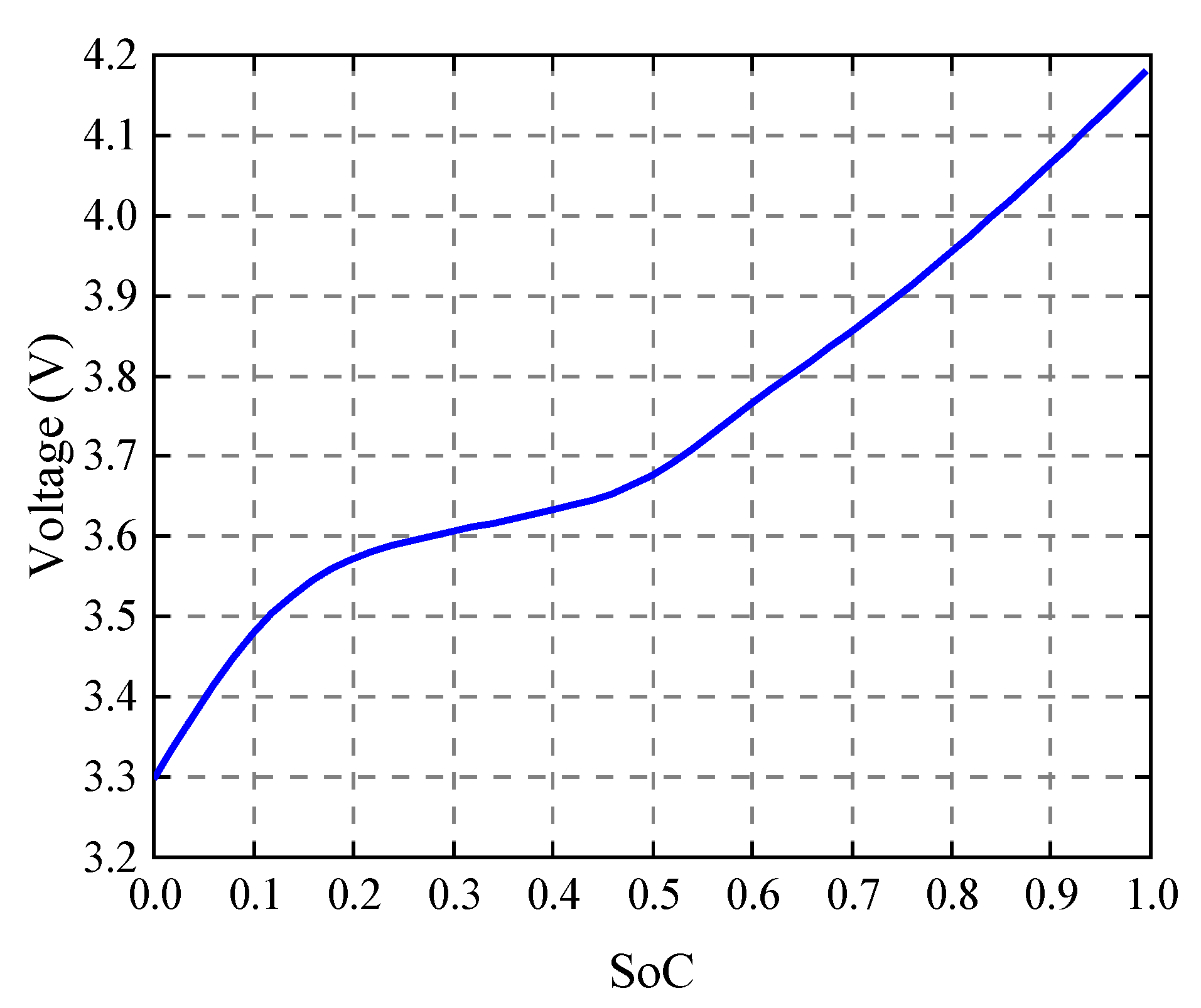
(1) The SoC-OCV relationship curve was fitted by the interval static method, as shown in Figure 2;

(2) The parameters of the second-order equivalent circuit model through DST test conditions were identified, as shown in Section 2.2 and Section 2.3;

(3) The MATLAB/SIMULINK block diagram of the four algorithms (UKF, CDKF, EKF, Proposed) was built;

(4) The SIMULINK block diagram of the algorithm was compiled and downloaded to the ControlDesk of dSPACE through the RTI model of SIMULINK;

(5) A virtual instrument for real-time estimation of lithium-ion battery SoC through ControlDesk was built;

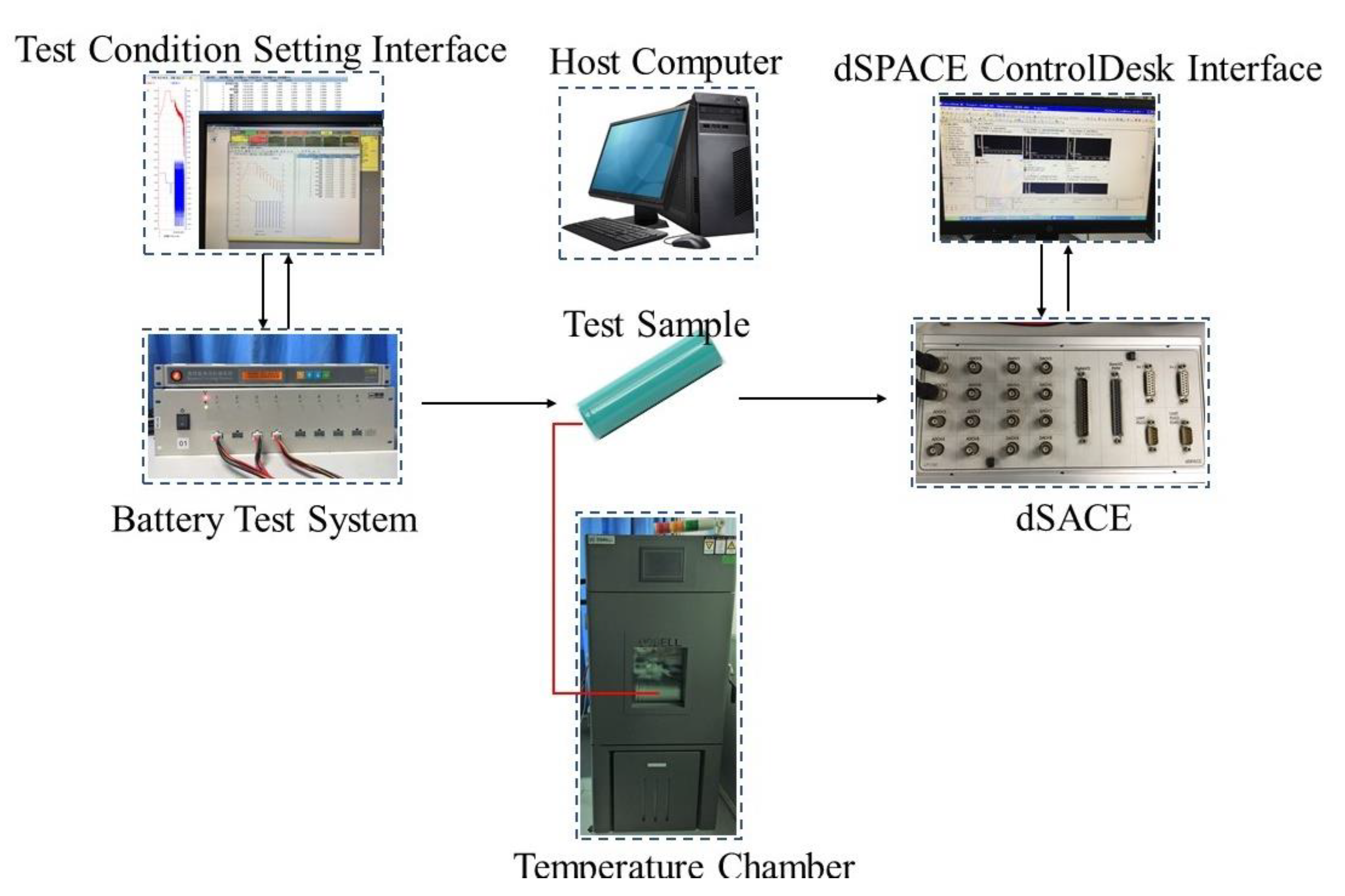
(6) The US06 and FUDS operating conditions were run through the battery test system, the current and voltage signals were collected in real-time through the current sensor and the DS1104 board, and the output voltage, voltage difference, SoC and SoC difference were displayed through the virtual instrument built by ControlDesk. The built-up battery test platform based on dSPACE is shown in Figure 6.

4.2. The Experimental Validation

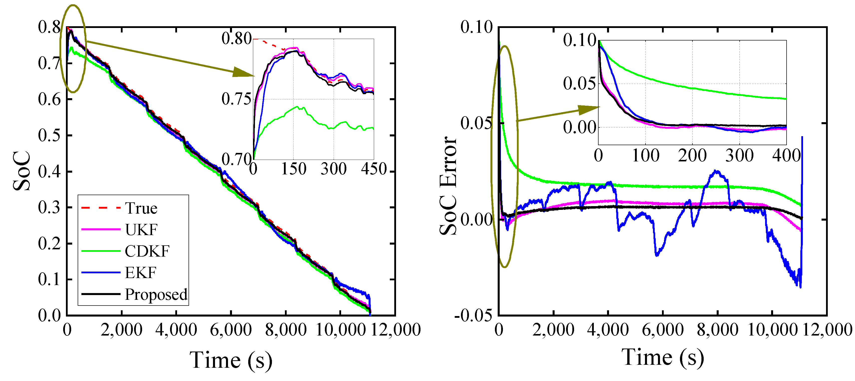
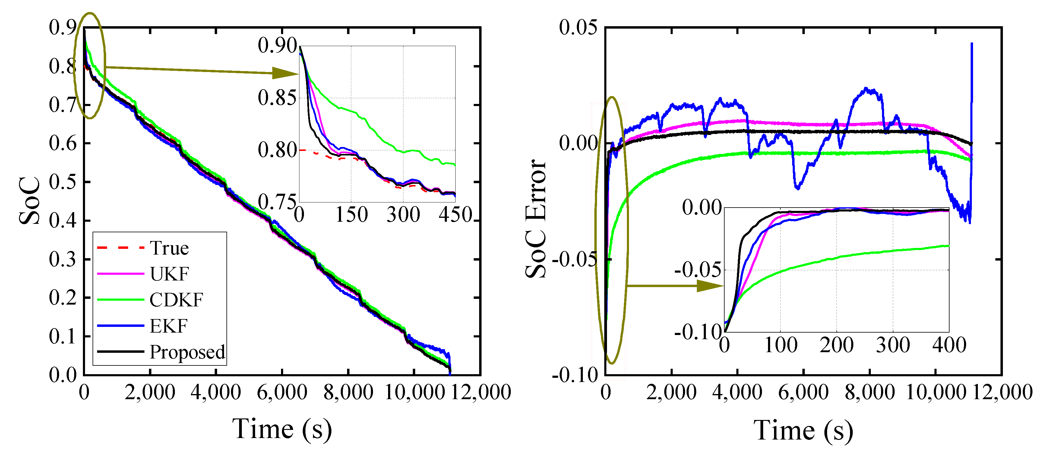
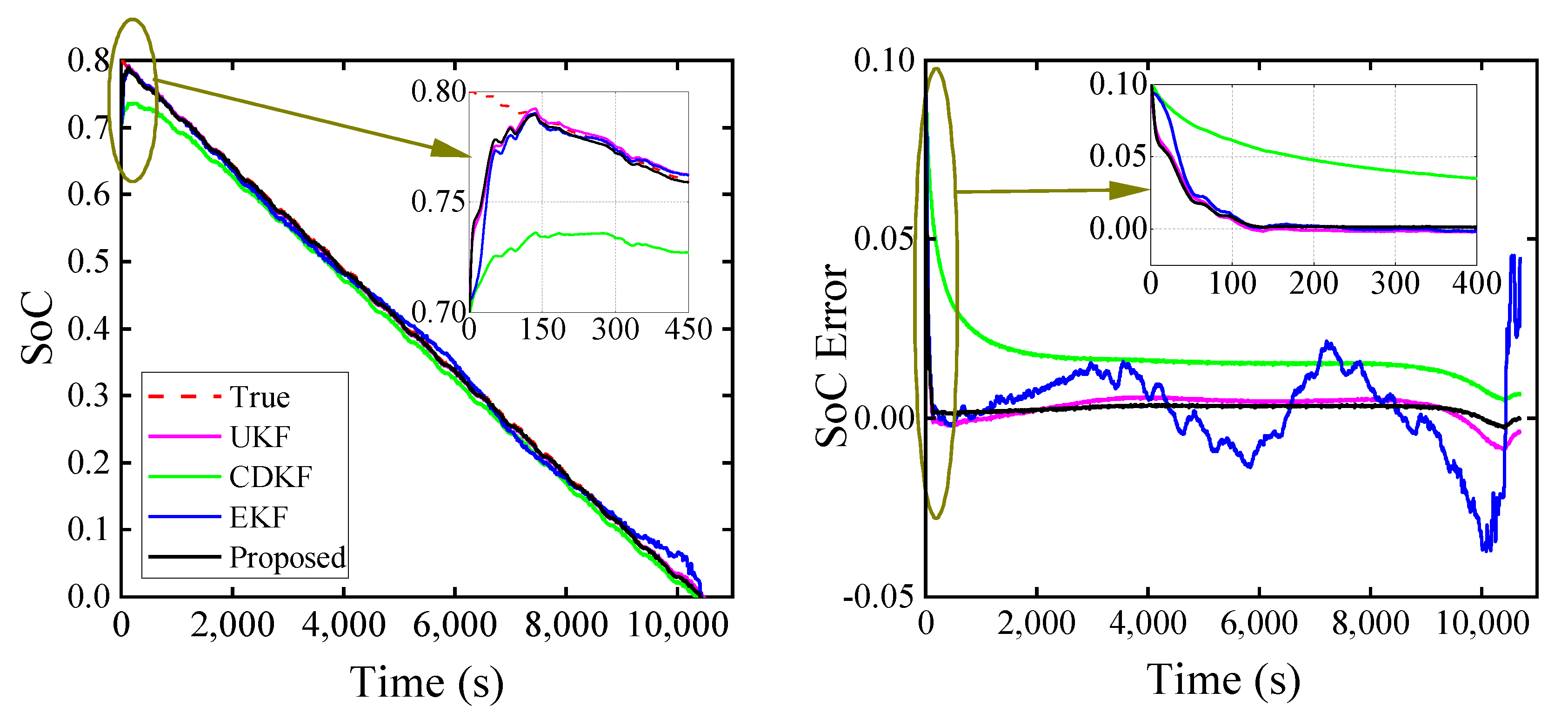
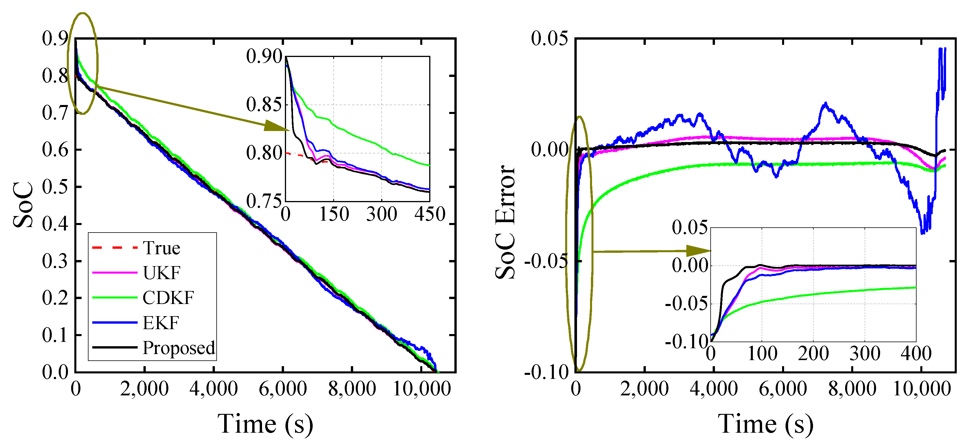
The battery test platform established in Section 4.1 was used to verify the ECM established in Section 2 of this article and the algorithm proposed in Section 3. We first charged the battery sample at constant current and constant voltage to the cut-off voltage of 4.2 V and let it stand for 1 h, discharged at 20% at constant current, and let it stand for another 1 h. At this moment, the initial value of the true SoC of the battery was 0.8. To verify the effectiveness of the proposed estimation method in the presence of initial SoC error, different hypothetical initial SoC values of 0.7 and 0.9 were set. The four algorithms, i.e., the proposed algorithm, UKF, CDKF and EKF, were used to estimate the SoC under FUDS and US06 charging and discharging conditions, respectively, and compare the initial error correction ability and robustness of the four algorithms. The charge and discharge test results of the battery are shown in

Table 5. Battery charge and discharge tests.

Test Serial Number	Condition	The Initial True SoC	The Initial SoC Guess
1	FUDS	0.8	0.7
2	FUDS	0.8	0.9
3	US06	0.8	0.7
4	US06	0.8	0.9

.

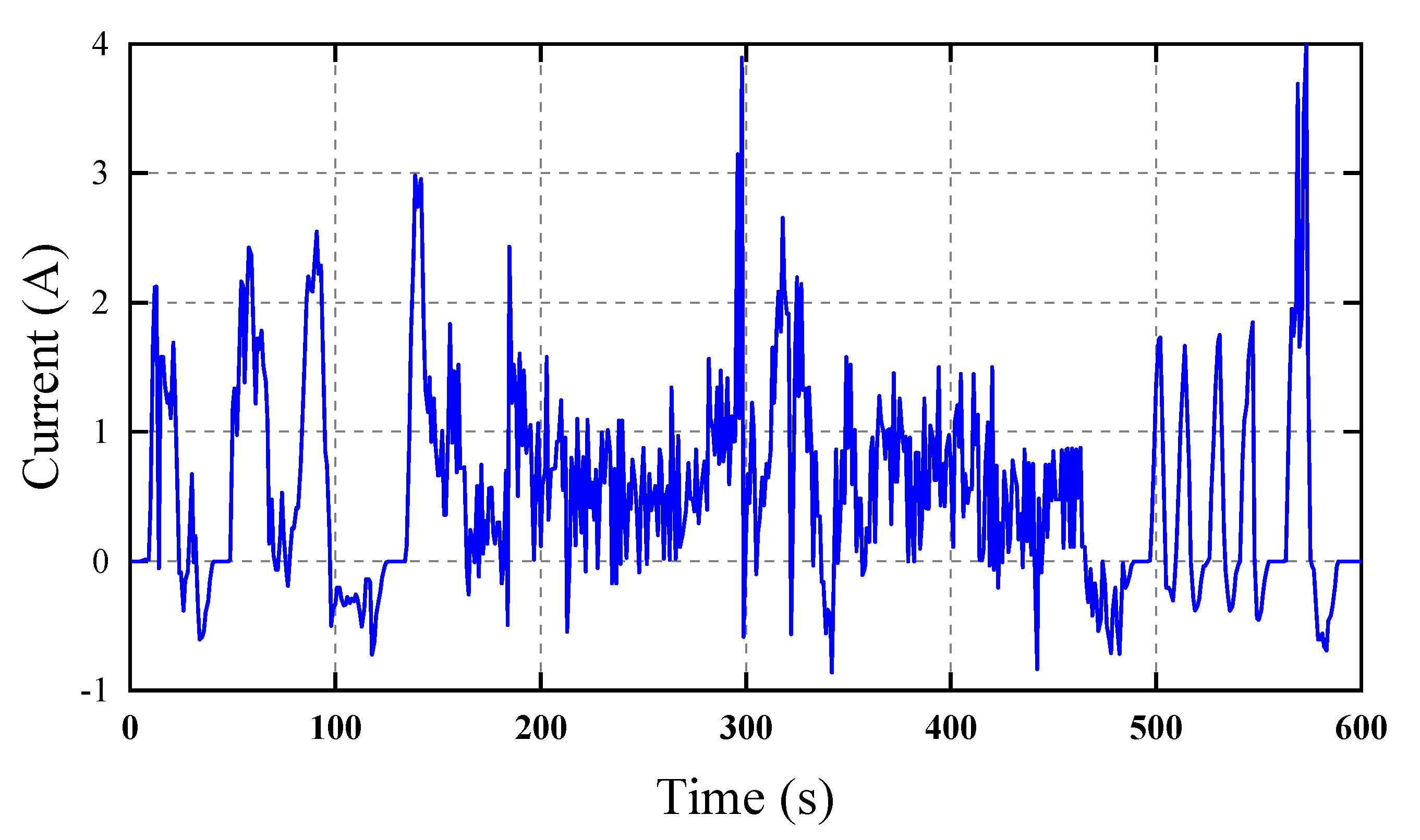
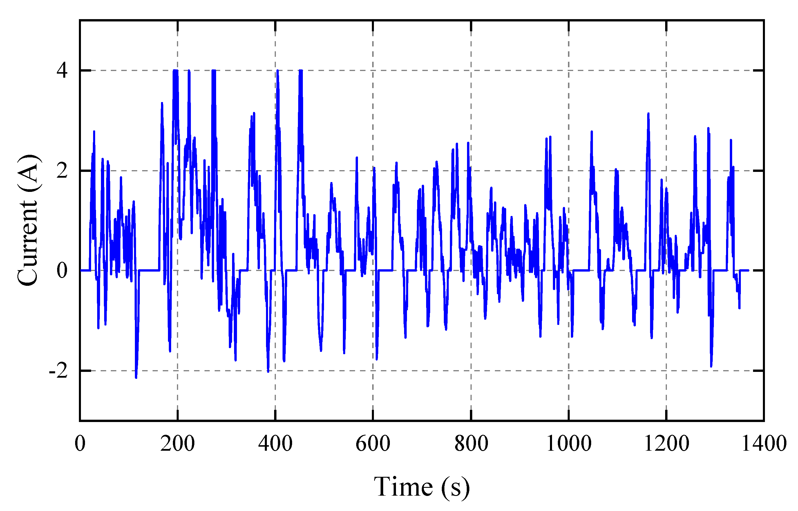
In order to verify the effectiveness of the proposed algorithm, the battery was tested under two dynamic conditions of US06 and FUDS. The US06 is a high acceleration aggressive driving schedule that is used by the United States Environmental Protection Agency for vehicle emissions and fuel economy testing [41]. The FUDS is an urban driving schedule based on an automobile industry standard [42]. The current of the battery constantly changes under dynamic working conditions, which can better simulate the actual operation of electric vehicles. Figure 7 show the current excitation of the battery under the US06 operating condition, and Figure 8 show the current excitation of the battery under the FUDS operating condition.

The battery SoC estimation and error results of the four algorithms are shown in Figure 9, Figure 10, Figure 11 and Figure 12.

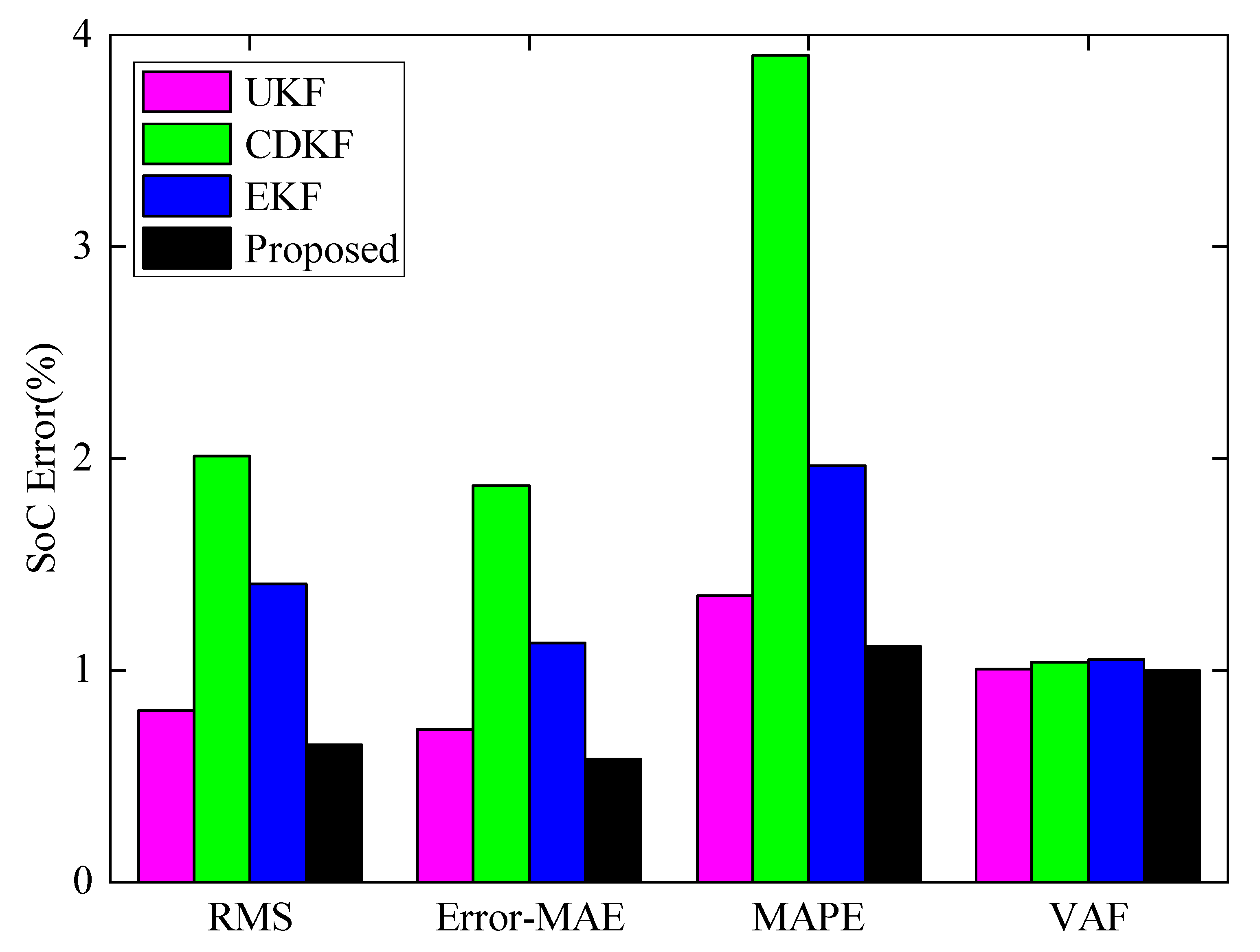
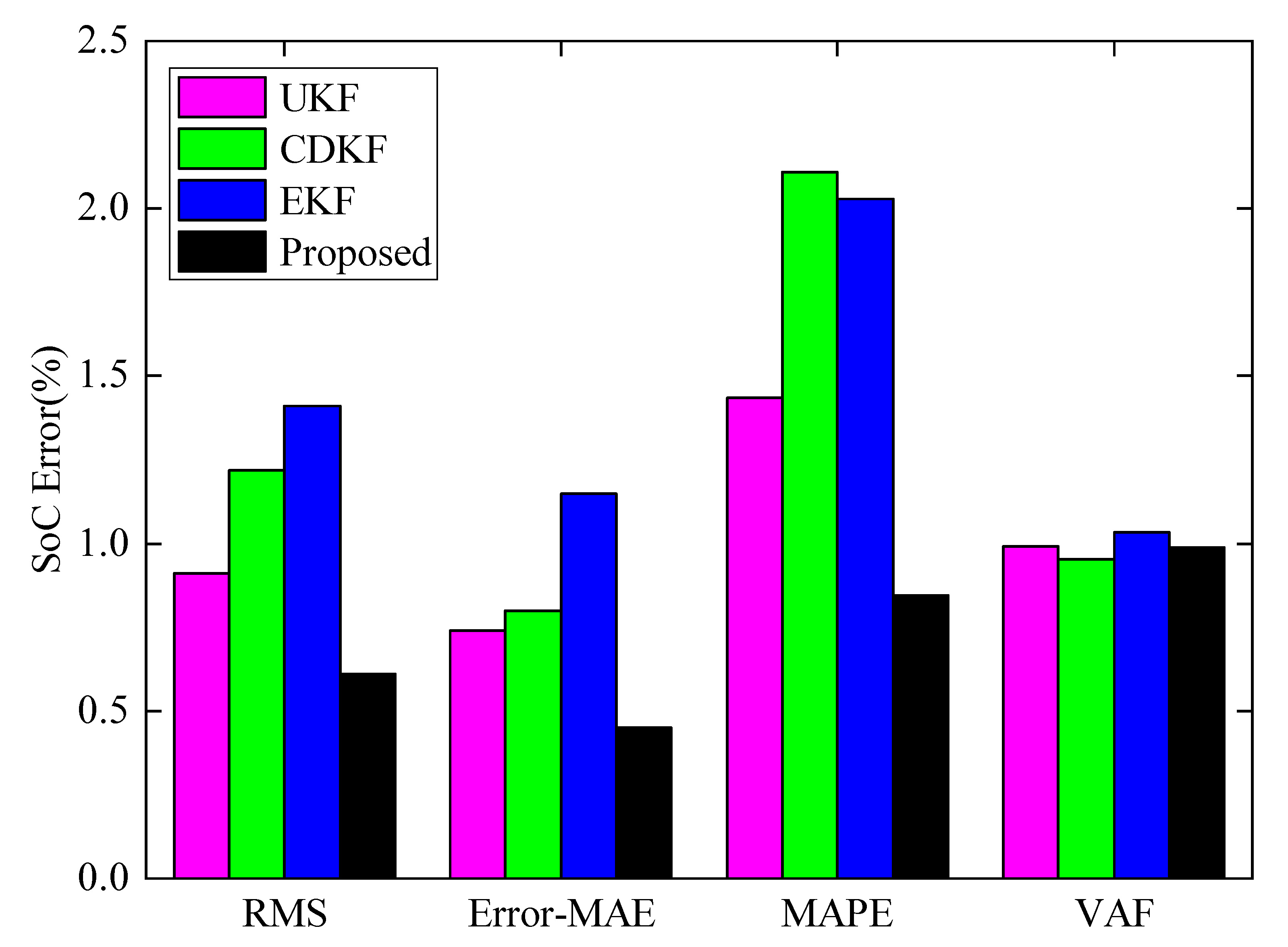
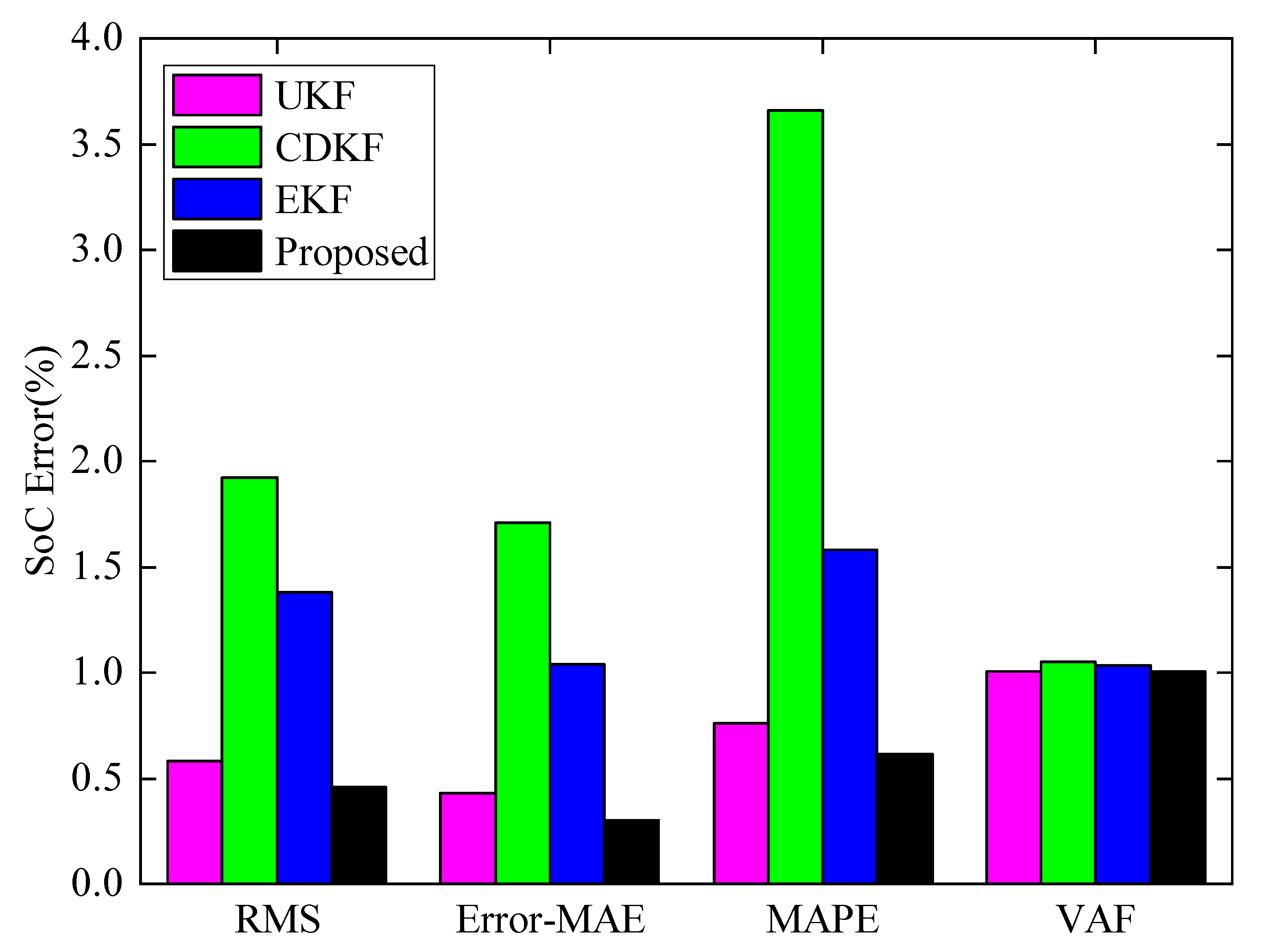
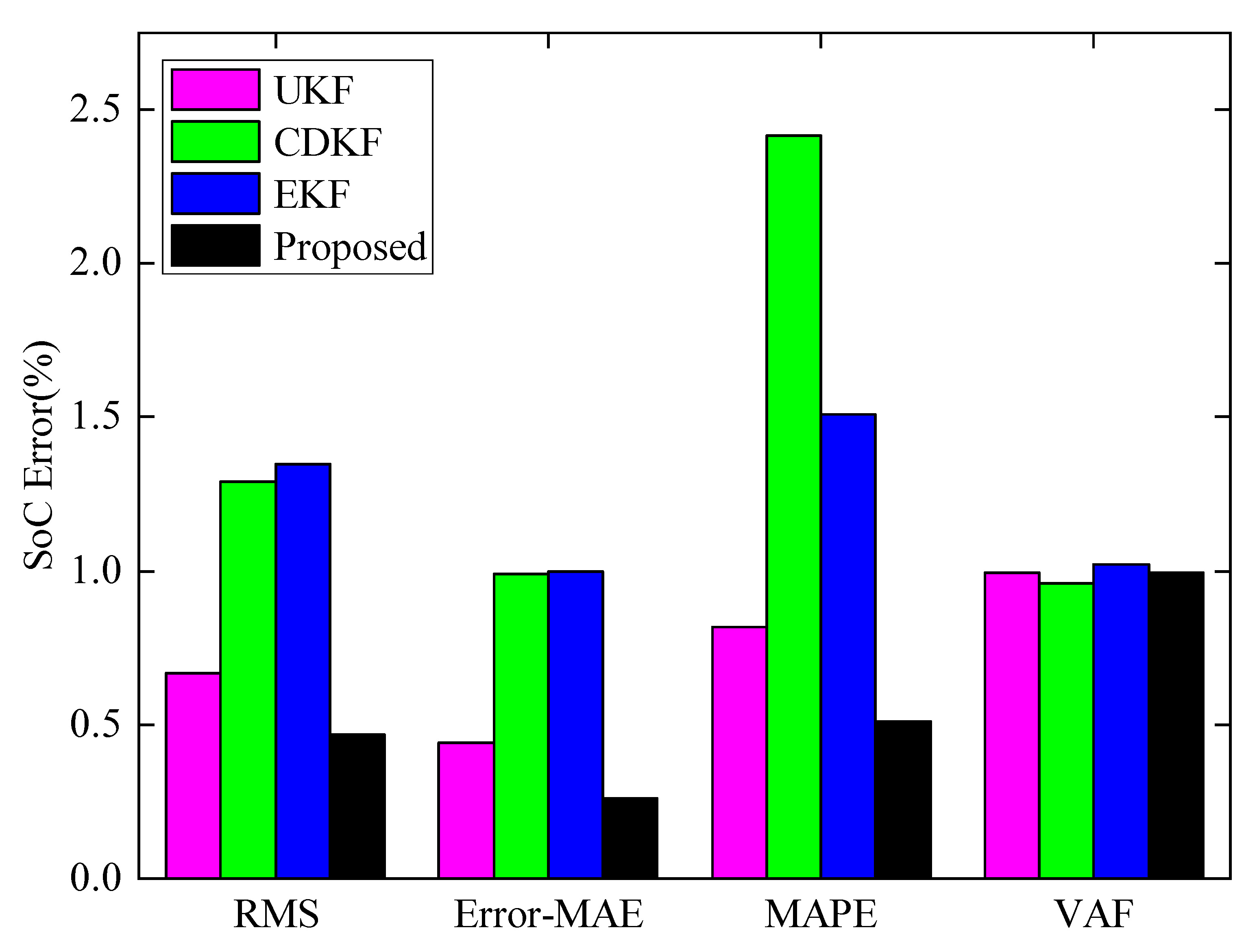
We used five evaluation indicators of RMS Error-MAE SI MAPE and VAF to further compare the SoC estimation effects of the four algorithms. The error comparison chart is shown in Figure 13, Figure 14, Figure 15 and Figure 16 where the root mean square error (RMS), average absolute error (Error-MAE), scattering index (SI), average absolute error percentage (MAPE) and variance (VAF) of the SoC is shown. The error results have been combined in

Table 6. Comparison of SoC estimation errors of four algorithms.

Condition	Algorithm	RMS	Error-MAE	SI	MAPE	VAF
The initial SoC guess was 0.7 under FUDS condition	UKF	0.0081	0.0072	0.0201	1.3542	1.0028
	CDKF	0.0201	0.0187	0.0503	3.9068	1.0404
	EKF	0.0141	0.0113	0.0353	1.9676	1.0500
	Proposed	0.0065	0.0058	0.0163	1.1100	1.0011
The initial SoC guess was 0.9 under FUDS condition	UKF	0.0091	0.0074	0.0227	1.4363	0.9906
	CDKF	0.0122	0.0080	0.0305	2.1100	0.9523
	EKF	0.0141	0.0115	0.0353	2.0290	1.0350
	Proposed	0.0061	0.0045	0.0153	0.8467	0.9884
The initial SoC guess was 0.7 under US06 condition	UKF	0.0058	0.0043	0.0149	0.7612	1.0071
	CDKF	0.0192	0.0171	0.0495	3.6600	1.0482
	EKF	0.0138	0.0104	0.0355	1.5805	1.0346
	Proposed	0.0046	0.0030	0.0119	0.6148	1.0052
The initial SoC guess was 0.9 under US06 condition	UKF	0.0067	0.0044	0.0173	0.8196	0.9956
	CDKF	0.0129	0.0099	0.0332	2.4148	0.9601
	EKF	0.0135	0.0100	0.0349	1.5113	1.0198
	Proposed	0.0047	0.0026	0.0120	0.5110	0.9964

Note: The true initial SoC value was 0.8.

. The time of initial error convergence is shown in

Table 7. The time of initial error convergence.

Condition	Algorithm	Time(s)
The initial SoC guess was 0.7 under FUDS condition	UKF	55
	CDKF	1595
	EKF	67
	Proposed	53
The initial SoC guess was 0.9 under FUDS condition	UKF	74
	CDKF	852
	EKF	68
	Proposed	44
The initial SoC guess was 0.7 under US06 condition	UKF	60
	CDKF	1377
	EKF	70
	Proposed	51
The initial SoC guess was 0.9 under US06 condition	UKF	66
	CDKF	831
	EKF	69
	Proposed	32

.

By analyzing Table 6 and Table 7, we can see that in the four conditions of the experiment, three evaluation indicators (RMS Error-MAE and SI) of CDKF and EKF were higher than the other two algorithms because these two algorithms approximate the posterior mean and covariance of the state with first-order accuracy. Compared with CDKF, the RMS of the proposed algorithm was reduced from 2.01%, 1.22%, 1.92%, 1.29% to 0.65%, 0.61%, 0.46%, 0.47%, respectively. The newly proposed algorithm could use the Sigma points in the UT transformation to approximate the posterior mean and covariance of the state with third-order Taylor accuracy in all four conditions. The calculation convergence time was close to that obtained with the UKF algorithm, achieving the effect of quickly correcting the initial error. The MAPE was found to be less than 2%. The VAF of the proposed algorithm ranked first three times and ranked second once (the initial SoC guess was 0.9 under the FUDS condition). The proposed algorithm showed better robustness in three of the four working conditions.

5. Conclusions

We proposed a graded round-robin SoC estimation method that combines UT transformation and Stirling interpolation center difference. In the first cycle, the Sigma points of the UT transformation were used to approximate the posterior mean value of the state with third-order Taylor accuracy to quickly correct the initial error of the SoC. This was helpful for the estimated SoC to converge to the reference value more quickly. The second cycle adopted the first-order truncated Stirling interpolation to obtain the approximation form of the function and did not need to calculate the Jacobian matrix, which effectively improved the calculation efficiency. By analyzing five evaluation indicators of RMS Error-MAE SI MAPE and VAF, the test results showed that the new algorithm guaranteed an SoC error within 2% under the FUDS and US06 working conditions, and it rapidly converged to the reference value within 60 s when the initial SoC value was inaccurate (±10%). In addition, the new algorithm showed better robustness in three of the four working conditions. Therefore, the proposed method could reduce the time for the SoC estimate value to converge to the reference value and ensure the accuracy and feasibility of lithium-ion battery SoC estimation.

References

- Poullikkas, A. Sustainable options for electric vehicle technologies. Renewable and Sustainable. Energy Rev. 2015, 41, 1277–1287. [Google Scholar]
- Xiong, R.; Sun, F.; Chen, Z.; He, H. A data-driven multi-scale extended Kalman filtering based parameter and state estimation approach of lithium-ion polymer battery in electric vehicles. Appl. Energy 2014, 113, 463–476. [Google Scholar] [CrossRef]
- Roscher, M.A.; Sauer, D.U. Dynamic electric behavior and open-circuit-voltage modeling of LiFePO4-based lithium ion secondary batteries. J. Power Sources 2011, 196, 331–336. [Google Scholar] [CrossRef]
- He, H.; Xiong, R.; Guo, H. Online estimation of model parameters and state-of-charge of LiFePO4 batteries in electric vehicles. Appl. Energy 2012, 89, 413–420. [Google Scholar] [CrossRef]
- Sun, F.; Hu, X.; Zou, Y.; Li, S. Adaptive unscented Kalman filtering for state of charge estimation of a lithium-ion battery for electric vehicles. Energy 2011, 36, 3531–3540. [Google Scholar] [CrossRef]
- Wang, D.; Miao, Q.; Pecht, M. Prognostics of lithium-ion batteries based on relevance vectors and a conditional three-parameter capacity degradation model. J. Power Sources 2013, 239, 253–264. [Google Scholar] [CrossRef]
- Kong, X.; Plett, G.L.; Trimboli, M.S.; Zhang, Z.; Qiao, D.; Zhao, T.; Zheng, Y. Pseudo-two-dimensional model and impedance diagnosis of micro internal short circuit in lithium-ion cells. J. Energy Storage 2020, 27, 101085. [Google Scholar] [CrossRef]
- Lu, L.; Han, X.; Li, J.; Hua, J.; Ouyang, M. A review on the key issues for lithium-ion battery management in electric vehicles. J. Power Sources 2013, 226, 272–288. [Google Scholar] [CrossRef]
- Barillas, J.K.; Li, J.; Günther, C.; Danzer, M.A. A comparative study and validation of state estimation algorithms for Li-ion batteries in battery management systems. Appl. Energy 2015, 155, 455–462. [Google Scholar] [CrossRef]
- Marongiu, A.; Nußbaum, F.G.W.; Waag, W.; Garmendia, M.; Sauer, D.U. Comprehensive study of the influence of aging on the hysteresis behavior of a lithium iron phosphate cathode-based lithium ion battery—An experimental investigation of the hysteresis. Appl. Energy 2016, 171, 629–645. [Google Scholar] [CrossRef]
- Han, X.; Ouyang, M.; Lu, L.; Li, J.; Zheng, Y.; Li, Z. A comparative study of commercial lithium ion battery cycle life in electrical vehicle: Aging mechanism identification. J. Power Sources 2014, 251, 38–54. [Google Scholar] [CrossRef]
- Weng, C.; Cui, Y.; Sun, J.; Peng, H. On-board state of health monitoring of lithium-ion batteries using incremental capacity analysis with support vector regression. J. Power Sources 2013, 235, 36–44. [Google Scholar] [CrossRef]
- Lavigne, L.; Sabatier, J.; Francisco, J.M.; Guillemard, F.; Noury, A. Lithium-ion Open Circuit Voltage (OCV) curve modelling and its ageing adjustment. J. Power Sources 2016, 324, 694–703. [Google Scholar] [CrossRef]
- Zhang, Y.; Song, W.; Lin, S.; Feng, Z. A novel model of the initial state of charge estimation for LiFePO4 batteries. J. Power Sources 2014, 248, 1028–1033. [Google Scholar] [CrossRef]
- Waag, W.; Sauer, D.U. Adaptive estimation of the electromotive force of the lithium-ion battery after current interruption for an accurate state-of-charge and capacity determination. Appl. Energy 2013, 111, 416–427. [Google Scholar] [CrossRef]
- Truchot, C.; Dubarry, M.; Liaw, B.Y. State-of-charge estimation and uncertainty for lithium-ion battery strings. Appl. Energy 2014, 119, 218–227. [Google Scholar] [CrossRef]
- Tang, X.; Wang, Y.; Chen, Z. A method for state-of-charge estimation of LiFePO4 batteries based on a dual-circuit state observer. J. Power Sources 2015, 296, 23–29. [Google Scholar] [CrossRef]
- Zhu, J.G.; Sun, Z.C.; Wei, X.Z.; Dai, H.F. A new lithium-ion battery internal temperature on-line estimate method based on electrochemical impedance spectroscopy measurement. J. Power Sources 2015, 274, 990–1004. [Google Scholar] [CrossRef]
- Waag, W.; Käbitz, S.; Sauer, D.U. Experimental investigation of the lithium-ion battery impedance characteristic at various conditions and aging states and its influence on the application. Appl. Energy 2013, 102, 885–897. [Google Scholar] [CrossRef]
- Wu, S.L.; Chen, H.C.; Chou, S.R. Fast estimation of state of charge for lithium-ion batteries. Energies 2014, 7, 3438–3452. [Google Scholar] [CrossRef]
- Doyle, M.; Newman, J.; Gozdz, A.S.; Schmutz, C.N.; Tarascon, J.M. Comparison of modeling predictions with experimental data from plastic lithium ion cells. J. Electrochem. Soc. 1996, 143, 1890–1903. [Google Scholar] [CrossRef]
- Doyle, M.; Fuller, T.F.; Newman, J. Modeling of galvanostatic charge and discharge of the lithium/polymer/insertion cell. J. Electrochem. Soc. 1993, 140, 1526–1533. [Google Scholar] [CrossRef]
- Ahmed, R.; Sayed, M.E.; Arasaratnam, I.; Tjong, J.; Habibi, S. Reduced-order electrochemical model parameters identification and state of charge estimation for healthy and aged Li-Ion Batteries-Part II: Aged battery model and state of charge estimation. IEEE J. Emerg. Sel. 2014, 678–690. [Google Scholar] [CrossRef]
- He, W.; Williard, N.; Chen, C.; Pecht, M. State of charge estimation for Li-ion batteries using neural network modeling and unscented Kalman filter-based error cancellation. Electr. Power Energy Syst. 2014, 62, 783–791. [Google Scholar] [CrossRef]
- Chen, C.; Xiong, R.; Yang, R.; Shen, W.; Sun, F. State-of-charge estimation of lithium-ion battery using an improved neural network model and extended Kalman filter. J. Clean. Prod. 2019, 234, 1153–1164. [Google Scholar] [CrossRef]
- Zahid, T.; Xu, K.; Li, W.; Li, C.; Li, H. State of charge estimation for electric vehicle power battery using advanced machine learning algorithm under diversified drive cycles. Energy 2018, 162, 871–882. [Google Scholar] [CrossRef]
- Tong, S.; Lacap, J.H.; Park, J.W. Battery state of charge estimation using a load-classifying neural network. J. Energy Storage 2016, 7, 236–243. [Google Scholar] [CrossRef]
- Bian, X.L.; Wei, Z.B.; Li, W.H.; Pou, J.; Sauer, D.U.; Liu, L.C. State-of-Health Estimation of Lithium-Ion Batteries by Fusing an Open Circuit Voltage Model and Incremental Capacity Analysis. IEEE Trans. Power Electron. 2021, 37, 2226–2236. [Google Scholar] [CrossRef]
- Bian, X.L.; Wei, Z.B.; He, J.T.; Yan, F.J.; Liu, L.C. A Novel Model-based Voltage Construction Method for Robust State-of-health Estimation of Lithium-ion Batteries. IEEE Trans. Ind. Electron. 2021, 68, 12173–12184. [Google Scholar] [CrossRef]
- Zhang, C.; Li, K.; Deng, J.; Song, S. Improved realtime state-of-charge estimation of LiFePO battery based on a novel thermoelectric model. IEEE T Ind. Electron. 2017, 64, 654–663. [Google Scholar] [CrossRef] [Green Version]
- Liu, C.; Liu, W.; Wang, L.; Hu, G.; Ma, L.; Ren, B. A new method of modeling and state of charge estimation of the battery. J. Power Sources 2016, 320, 1–12. [Google Scholar] [CrossRef]
- Shen, M. A review on battery management system from the modeling efforts to its multiapplication and integration. Int. J. Energy Res. 2019, 43, 5042–5075. [Google Scholar] [CrossRef]
- Bian, X.L.; Wei, Z.B.; He, J.T.; Yan, F.J.; Liu, L.C. A two-step parameter optimization method for low-order model-based state of charge estimation. IEEE Trans. Transp. Electrif. 2021, 7, 399–409. [Google Scholar] [CrossRef]
- Li, J.; Wang, L.; Lyu, C.; Pecht, M. State of charge estimation based on a simplified electrochemical model for a single LiCoO2 battery and battery pack. Energy 2017, 133, 572–583. [Google Scholar] [CrossRef]
- Plett, G.L. Sigma-point Kalman filtering for battery management systems of LiPB-based HEV battery packs, Part 1: Introduction and state estimation. J. Power Sources 2006, 161, 1356–1368. [Google Scholar] [CrossRef]
- Plett, G.L. Sigma-point Kalman filtering for battery management systems of LiPB-based HEV battery packs, Part 2: Simultaneous state and parameter estimation. J. Power Sources 2006, 161, 1369–1384. [Google Scholar] [CrossRef]
- Schei, T.S. A finite-difference method for linearization in nonlinear estimation algorithms. Automatic 1997, 11, 2053–2058. [Google Scholar] [CrossRef]
- Ito, K.; Xiong, K. Gaussian filters for nonlinear filtering problems. IEEE Trans. Autom. Control 2000, 5, 910–927. [Google Scholar] [CrossRef] [Green Version]
- Nørgaard, M.; Poulsen, N.K.; Ravn, O. Advances in Derivative-Free State Estimation for Nonlinear Systems; Technical Report: IMM-REP-1998-15; Technical University of Denmark: Lyngby, Denmark, 2000. [Google Scholar]
- Merwe, R.V. Sigma-Point Kalman Filters for Probalilistic Inference in Dynamic State-Space Models. Ph.D. Thesis, Oregon Health & Science University, Beaverton, OR, USA, 2004. [Google Scholar]
- Dynamometer Drive Schedules. Available online: https://www.epa.gov/vehicle-and-fuel-emissions-testing/dynamometer-drive-schedules (accessed on 15 October 2020).
- USABC Electric Vehicle Battery Test Procedures Manual. Revision 2. Available online: https://digital.library.unt.edu/ark:/67531/metadc666152/m1/24/ (accessed on 16 October 2020).
Figure 1.
Schedule of the charge and discharge tests.
Figure 2.
SoC-OCV mapping curve.
Figure 3.
The 2-RC ECM.
Figure 4.
Current excitation curve under DST condition.
Figure 5.
Flow chart of the proposed algorithm.
Figure 6.
Real-time SoC estimation platform based on dSPACE Rapid Prototyping Systems.
Figure 7.
Battery current excitation curve under the US06 working condition.
Figure 8.
Battery current excitation curve under the FUDS working condition.
Figure 9.
The initial SoC guess was 0.7 under the FUDS condition.
Figure 10.
The initial SoC guess was 0.9 under the FUDS condition.
Figure 11.
The initial SoC guess was 0.7 under the US06 condition.
Figure 12.
The initial SoC guess was 0.9 under the US06 condition.
Figure 13.
The four evaluation indexes of the initial SoC guess were 0.7 under the FUDS condition.
Figure 14.
The four evaluation indexes of the initial SoC guess were 0.9 under the FUDS condition.
Figure 15.
The four evaluation indexes of the initial SoC guess were 0.7 under the US06 condition.
Figure 16.
The four evaluation indexes of the initial SoC guess were 0.9 under the US06 condition.