
Mallard Detection Using Microphone Arrays Combined with Delay-and-Sum Beamforming for Smart and Remote Rice–Duck Farming

 , , and
Abstract
:1. Introduction
2. Related Studies
- The proposed method can detect the position of a sound source of pre-recorded mallard calls output from a speaker using two parameters obtained from our originally developed microphone arrays;
- Compared with existing sound-based methods, our study results provide a detailed evaluation that comprises 57 positions in total through three evaluation experiments;
- To the best of our knowledge, this is the first study to demonstrate and evaluate mallard detection based on DAS beamforming in the wild.
3. Proposed Method
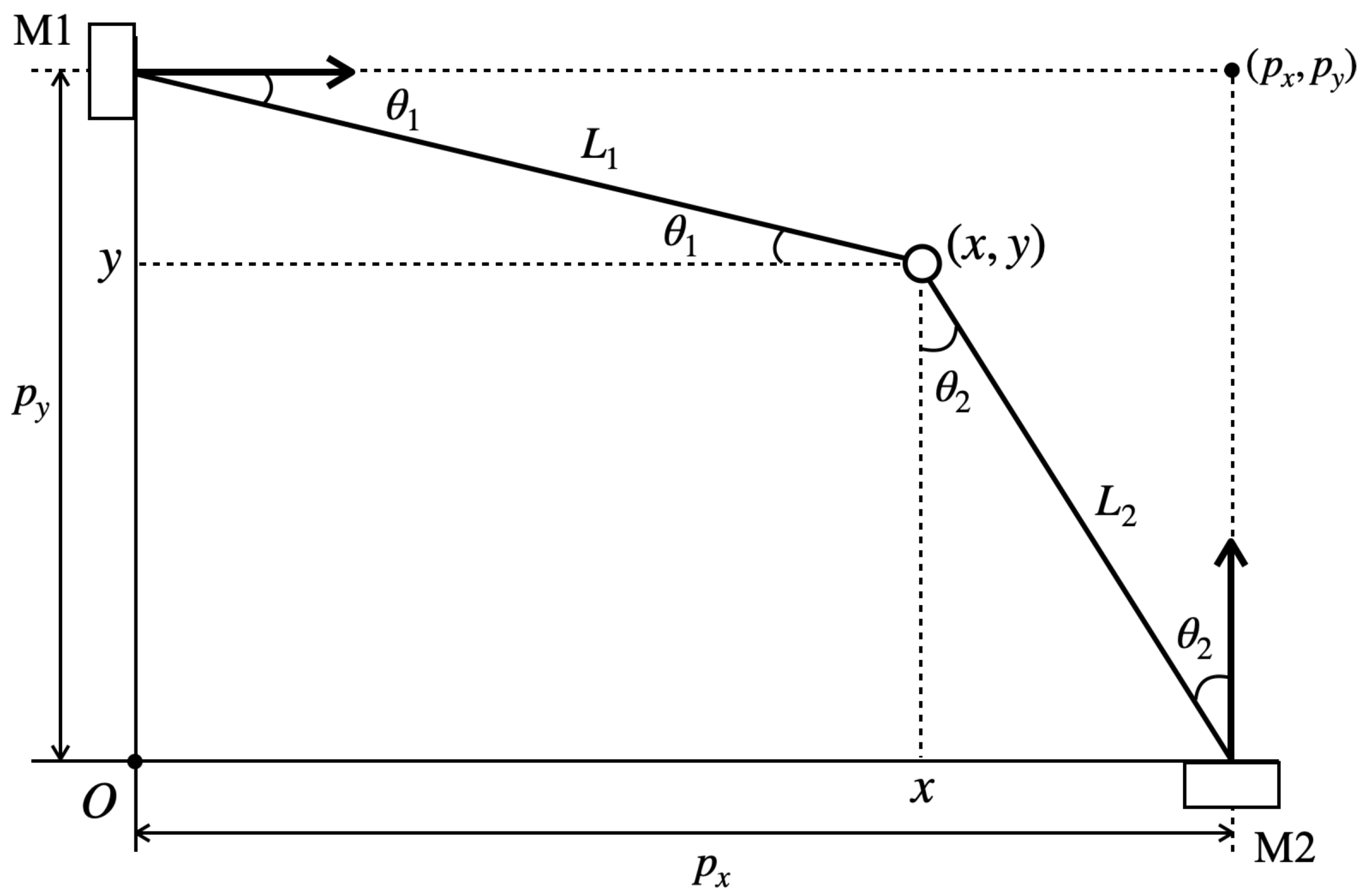
3.1. Position Estimation Principle
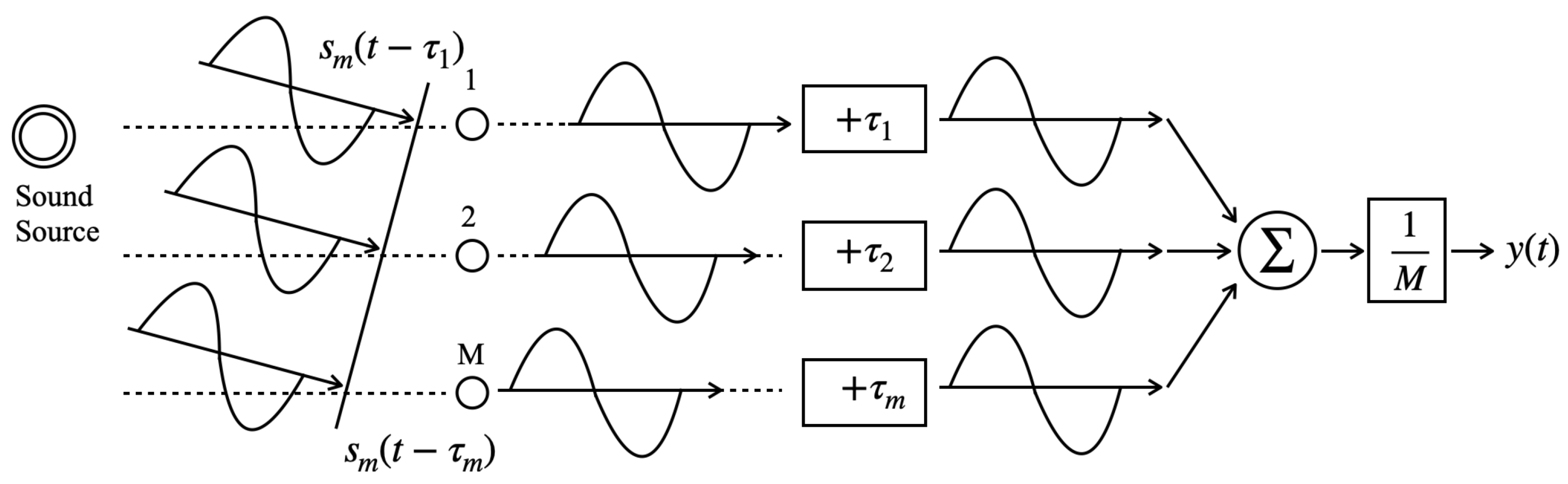
3.2. DAS Beamforming Algorithm
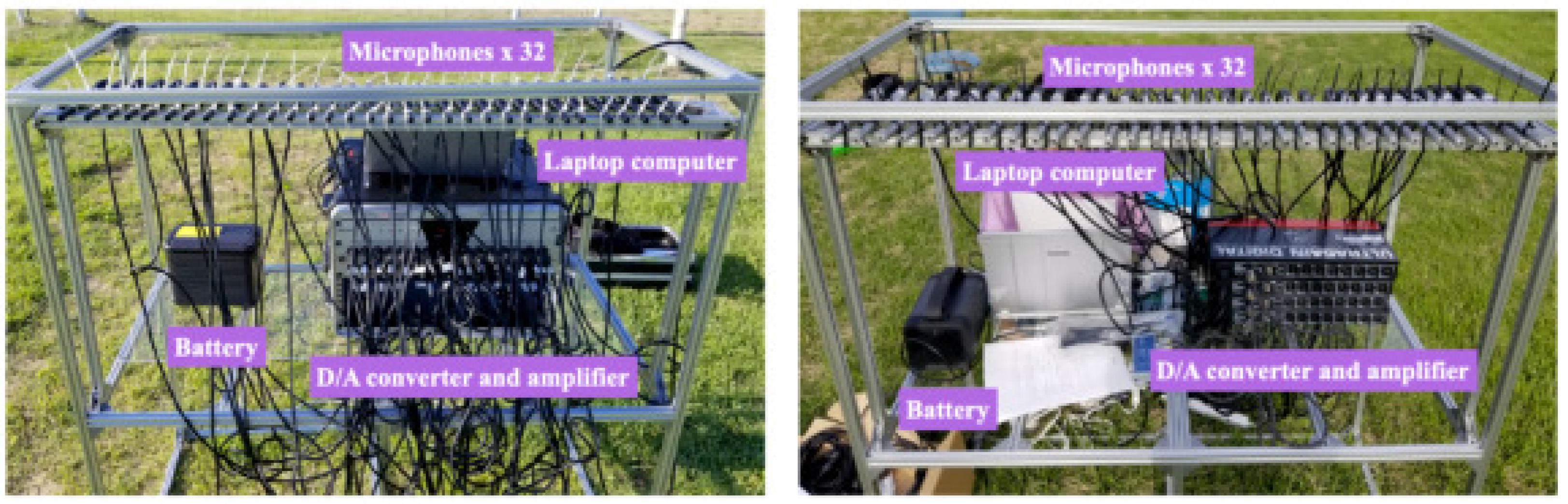
4. Measurement System
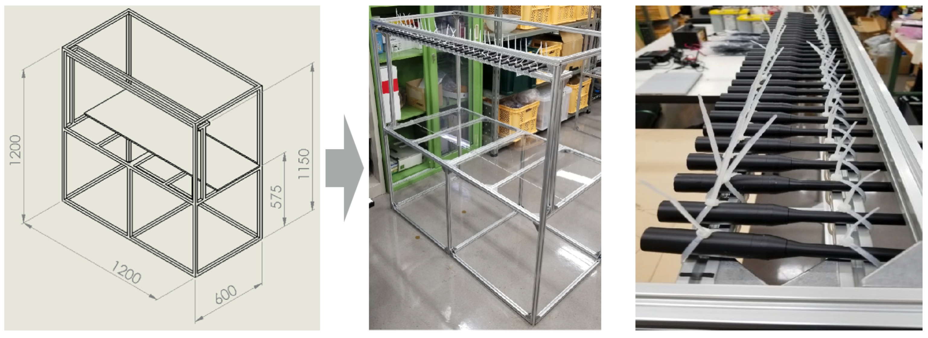
4.1. Mount Design
4.2. Microphone Array
5. Evaluation Experiment
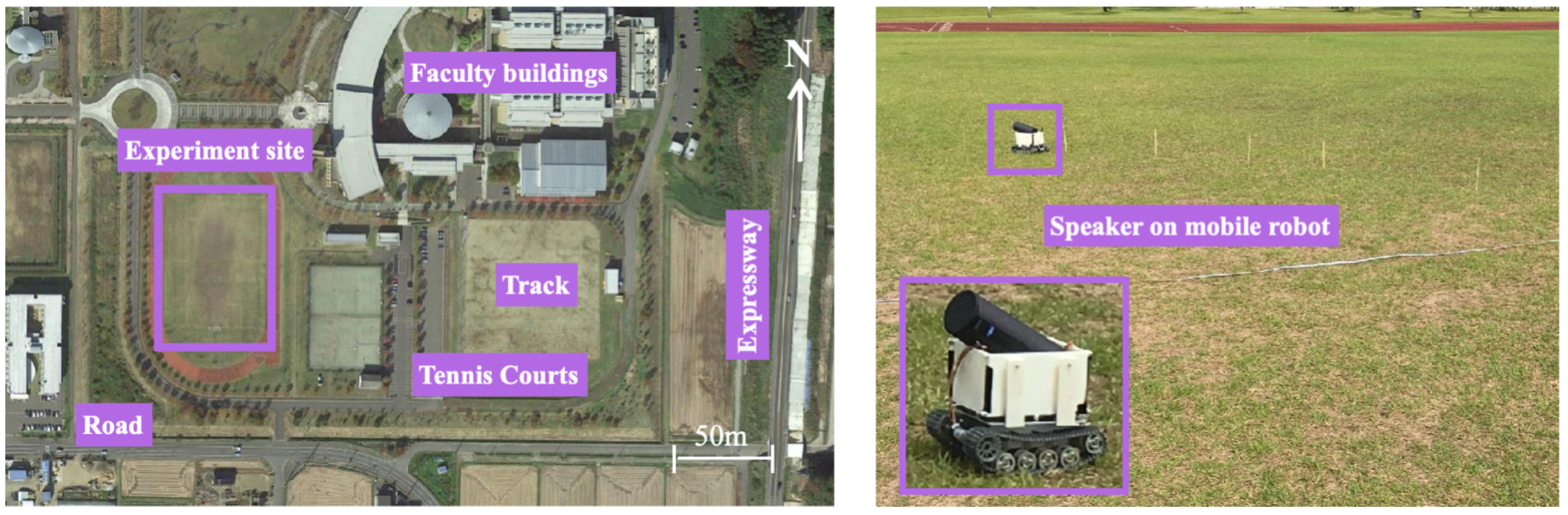
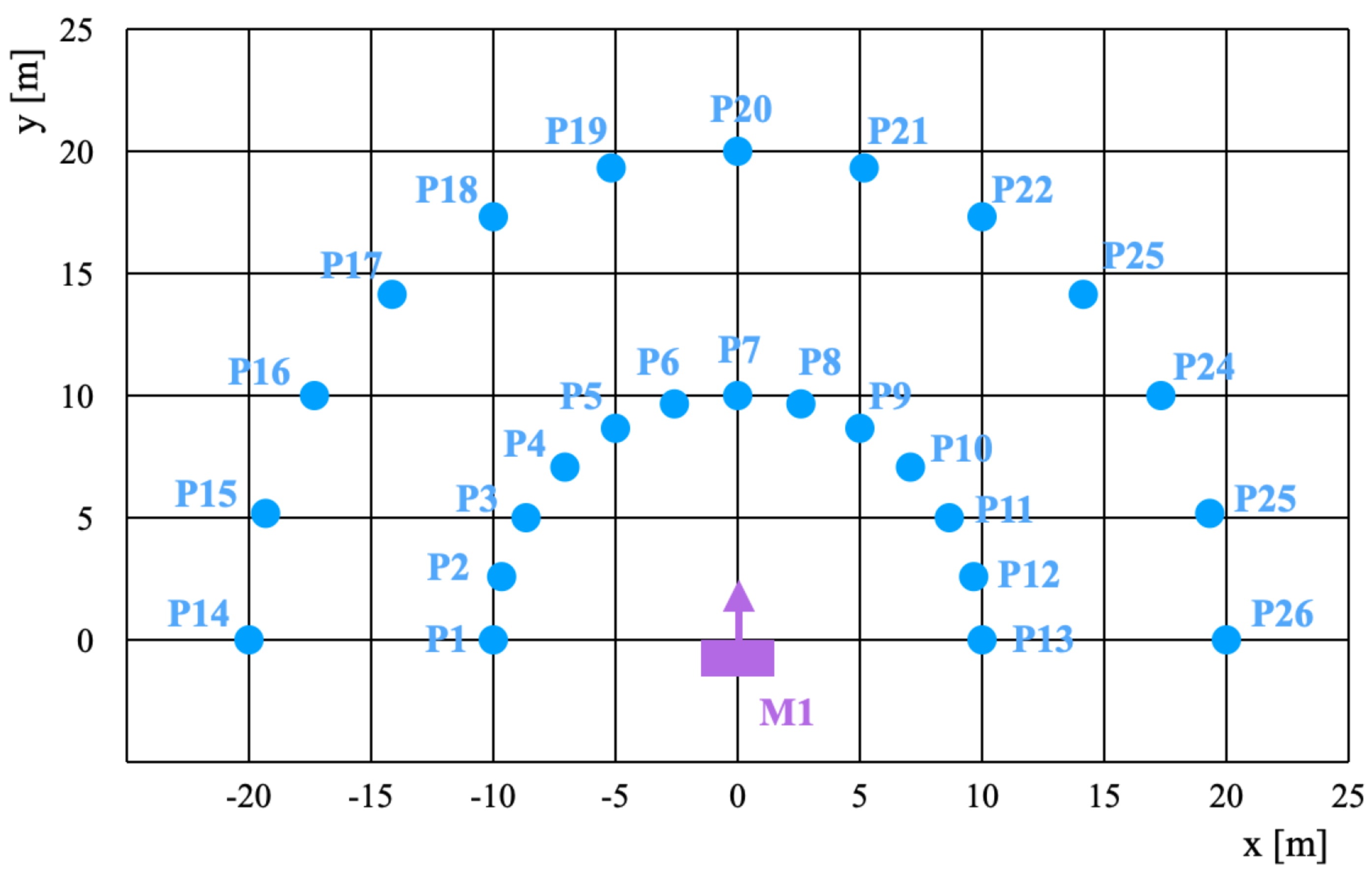
5.1. Experiment Setup
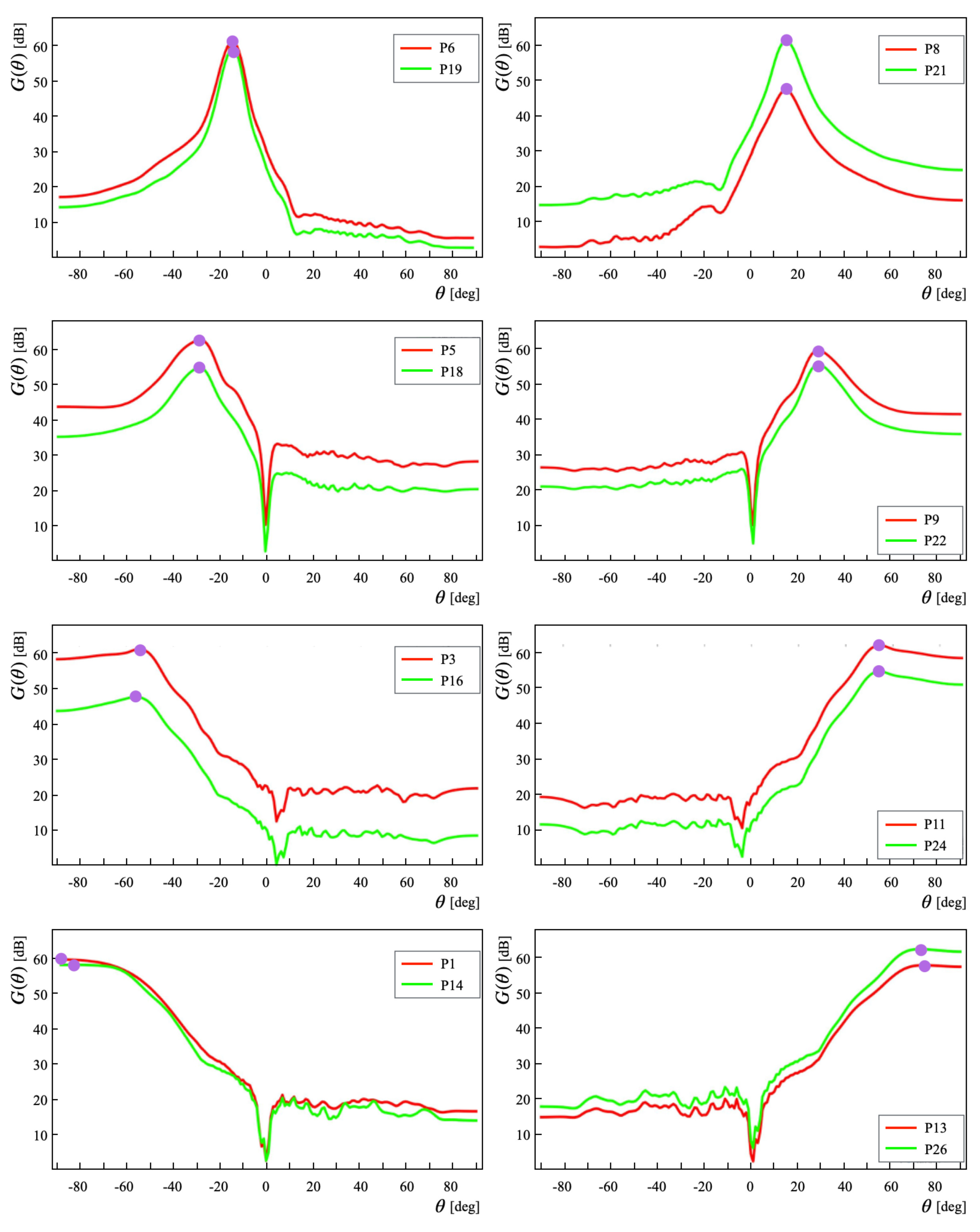
5.2. Experiment A
5.3. Experiment B
5.4. Experiment C
5.5. Discussion
6. Conclusions
Author Contributions
Funding
Institutional Review Board Statement
Informed Consent Statement
Data Availability Statement
Acknowledgments
Conflicts of Interest
Abbreviations
| AD | analog-to-digital |
| AVSS | advanced video and signal-based surveillance |
| BoF | bag-of-features |
| BS | background subtraction |
| CNN | convolutional neural network |
| DAS | delay-and-sum |
| DBDC | Drone-vs-Bird Detection Challenge |
| DCASE | detection and classification of acoustic scenes and events |
| DC-CNN | densely connected convolutional neural network |
| DL | deep learning |
| EM | expectation–maximization |
| GAN | generative adversarial network |
| GMM | Gaussian mixture models |
| HOG | histogram of oriented gradients |
| JST | Japan Standard Time |
| LBP | local binary pattern |
| MF | morphological filtering |
| MIML | multi-instance, multi-label |
| ML | machine learning |
| PCA | principal component analysis |
| RCNN | regions with convolutional neural network |
| RF | random forest |
| SIFT | scale-invariant features transform |
| SVM | support vector machine |
| UGV | unmanned ground vehicle |
| UTC | Coordinated Universal Time |
| WS-DAN | weakly supervised data augmentation network |
| YOLO | you only look once |
References
- Hossain, S.; Sugimoto, H.; Ahmed, G.; Islam, M. Effect of Integrated Rice-Duck Farming on Rice Yield, Farm Productivity, and Rice-Provisioning Ability of Farmers. Asian J. Agric. Dev. 2005, 2, 79–86. [Google Scholar]
- Madokoro, H.; Yamamoto, S.; Nishimura, Y.; Nix, S.; Woo, H.; Sato, K. Prototype Development of Small Mobile Robots for Mallard Navigation in Paddy Fields: Toward Realizing Remote Farming. Robotics 2021, 10, 63. [Google Scholar] [CrossRef]
- Reiher, C.; Yamaguchi, T. Food, agriculture and risk in contemporary Japan. Contemp. Jpn. 2017, 29, 2–13. [Google Scholar] [CrossRef]
- Lack, D.; Varley, G. Detection of Birds by Radar. Nature 1945, 156, 446. [Google Scholar] [CrossRef]
- Chabot, D.; Francis, C.M. Computer-automated bird detection and counts in high-resolution aerial images: A review. J. Field Ornithol. 2016, 87, 343–359. [Google Scholar] [CrossRef]
- Goel, S.; Bhusal, S.; Taylor, M.E.; Karkee, M. Detection and Localization of Birds for Bird Deterrence Using UAS. In Proceedings of the 2017 ASABE Annual International Meeting, Spokane, WA, USA, 16–19 July 2017. [Google Scholar]
- Siahaan, Y.; Wardijono, B.A.; Mukhlis, Y. Design of Birds Detector and Repellent Using Frequency Based Arduino Uno with Android System. In Proceedings of the 2017 2nd International Conference on Information Technology, Information Systems and Electrical Engineering (ICITISEE), Yogyakarta, Indonesia, 1–3 November 2017; pp. 239–243. [Google Scholar]
- Aishwarya, K.; Kathryn, J.C.; Lakshmi, R.B. A Survey on Bird Activity Monitoring and Collision Avoidance Techniques in Windmill Turbines. In Proceedings of the 2016 IEEE Technological Innovations in ICT for Agriculture and Rural Development, Chennai, India, 15–16 July 2016; pp. 188–193. [Google Scholar]
- Bas, Y.; Bas, D.; Julien, J.F. Tadarida: A Toolbox for Animal Detection on Acoustic Recordings. J. Open Res. Softw. 2017, 5, 6. [Google Scholar] [CrossRef] [Green Version]
- Dong, X.; Jia, J. Advances in Automatic Bird Species Recognition from Environmental Audio. J. Phys. Conf. Ser. 2020, 1544, 012110. [Google Scholar] [CrossRef]
- Kahl, S.; Clapp, M.; Hopping, W.; Goëau, H.; Glotin, H.; Planqué, R.; Vellinga, W.P.; Joly, A. Overview of BirdCLEF 2020: Bird Sound Recognition in Complex Acoustic Environments. In Proceedings of the 11th International Conference of the Cross-Language Evaluation Forum for European Languages, Thessaloniki, Greece, 20–25 September 2020. [Google Scholar]
- Qing, C.; Dickinson, P.; Lawson, S.; Freeman, R. Automatic nesting seabird detection based on boosted HOG-LBP descriptors. In Proceedings of the 18th IEEE International Conference on Image, Brussels, Belgium, 11–14 September 2011; pp. 3577–3580. [Google Scholar]
- Descamps, S.; B’echet, A.; Descombes, X.; Arnaud, A.; Zerubia, J. An Automatic Counter for Aerial Images of Aggregations of Large Birds. Bird Study 2011, 58, 302–308. [Google Scholar] [CrossRef]
- Farrell, R.; Oza, O.; Zhang, N.; Morariu, V.I.; Darrell, T.; Davis, L.S. Birdlets: Subordinate categorization using volumetric primitives and pose-normalized appearance. In Proceedings of the International Conference on Computer Vision, Barcelona, Spain, 6–13 November 2011; pp. 161–168. [Google Scholar]
- Mihreteab, K.; Iwahashi, M.; Yamamoto, M. Crow birds detection using HOG and CS-LBP. In Proceedings of the International Symposium on Intelligent Signal Processing and Communications Systems, New Taipei City, Taiwan, 4–7 November 2012. [Google Scholar]
- Liu, J.; Belhumeur, P.N. Bird Part Localization Using Exemplar-Based Models with Enforced Pose and Subcategory Consistency. In Proceedings of the IEEE International Conference on Computer Vision, Sydney, Australia, 3–6 December 2013; pp. 2520–2527. [Google Scholar]
- Xu, Q.; Shi, X. A simplified bird skeleton based flying bird detection. In Proceedings of the 11th World Congress on Intelligent Control and Automation, Shenyang, China, 27–30 June 2014; pp. 1075–1078. [Google Scholar]
- Yoshihashi, R.; Kawakami, R.; Iida, M.; Naemura, T. Evaluation of Bird Detection Using Time-Lapse Images around a Wind Farm. In Proceedings of the European Wind Energy Association Conference, Paris, France, 17–20 November 2015. [Google Scholar]
- T’Jampens, R.; Hernandez, F.; Vandecasteele, F.; Verstockt, S. Automatic detection, tracking and counting of birds in marine video content. In Proceedings of the Sixth International Conference on Image Processing Theory, Tools and Applications, Oulu, Finland, 12–15 December 2016; pp. 1–6. [Google Scholar]
- Takeki, A.; Trinh, T.T.; Yoshihashi, R.; Kawakami, R.; Iida, M.; Naemura, T. Combining Deep Features for Object Detection at Various Scales: Finding Small Birds in Landscape Images. IPSJ Trans. Comput. Vis. Appl. 2016, 8, 5. [Google Scholar] [CrossRef] [Green Version]
- Takeki, A.; Trinh, T.T.; Yoshihashi, R.; Kawakami, R.; Iida, M.; Naemura, T. Detection of Small Birds in Large Images by Combining a Deep Detector with Semantic Segmentation. In Proceedings of the 2016 IEEE International Conference on Image Processing, Phoenix, AR, USA, 25–28 September 2016; pp. 3977–3981. [Google Scholar]
- Yoshihashi, R.; Kawakami, R.; Iida, M.; Naemura, T. Bird Detection and Species Classification with Time-Lapse Images around a Wind Farm: Dataset Construction and Evaluation. Wind Energy 2017, 20, 1983–1995. [Google Scholar] [CrossRef]
- Tian, S.; Cao, X.; Zhang, B.; Ding, Y. Learning the State Space Based on Flying Pattern for Bird Detection. In Proceedings of the 2017 Integrated Communications, Navigation and Surveillance Conference, Herndon, VA, USA, 18–20 April 2017; pp. 5B3-1–5B3-9. [Google Scholar]
- Wu, T.; Luo, X.; Xu, Q. A new skeleton based flying bird detection method for low-altitude air traffic management. Chin. J. Aeronaut. 2018, 31, 2149–2164. [Google Scholar] [CrossRef]
- Lee, S.; Lee, M.; Jeon, H.; Smith, A. Bird Detection in Agriculture Environment using Image Processing and Neural Network. In Proceedings of the 6th International Conference on Control, Decision and Information Technologies, Paris, France, 23–26 April 2019; pp. 1658–1663. [Google Scholar]
- Vishnuvardhan, R.; Deenadayalan, G.; Vijaya Gopala Rao, M.V.; Jadhav, S.P.; Balachandran, A. Automatic Detection of Flying Bird Species Using Computer Vision Techniques. In Proceedings of the International Conference on Physics and Photonics Processes in Nano Sciences, Eluru, India, 20–22 June 2019. [Google Scholar]
- Hong, S.J.; Han, Y.; Kim, S.Y.; Lee, A.Y.; Kim, G. Application of Deep-Learning Methods to Bird Detection Using Unmanned Aerial Vehicle Imagery. Sensors 2019, 19, 1651. [Google Scholar] [CrossRef] [PubMed] [Green Version]
- Boudaoud, L.B.; Maussang, F.; Garello, R.; Chevallier, A. Marine Bird Detection Based on Deep Learning using High-Resolution Aerial Images. In Proceedings of the OCEANS 2019—Marseille, Marseille, France, 17–20 June 2019; pp. 1–7. [Google Scholar]
- Jo, J.; Park, J.; Han, J.; Lee, M.; Smith, A.H. Dynamic Bird Detection Using Image Processing and Neural Network. In Proceedings of the 7th International Conference on Robot Intelligence Technology and Applications, Daejeon, Korea, 1–3 November 2019; pp. 210–214. [Google Scholar]
- Fan, J.; Liu, X.; Wang, X.; Wang, D.; Han, M. Multi-Background Island Bird Detection Based on Faster R-CNN. Cybern. Syst. 2020, 52, 26–35. [Google Scholar] [CrossRef]
- Akcay, H.G.; Kabasakal, B.; Aksu, D.; Demir, N.; Öz, M.; Erdoǧan, A. Automated Bird Counting with Deep Learning for Regional Bird Distribution Mapping. Animals 2020, 10, 1207. [Google Scholar] [CrossRef]
- Mao, X.; Chow, J.K.; Tan, P.S.; Liu, K.; Wu, J.; Su, Z.; Cheong, Y.H.; Ooi, G.L.; Pang, C.C.; Wang, Y. Domain Randomization-Enhanced Deep Learning Models for Bird Detection. Sci. Rep. 2021, 11, 639. [Google Scholar] [CrossRef]
- Marcoň, P.; Janoušek, J.; Pokorný, J.; Novotný, J.; Hutová, E.V.; Širůčková, A.; Čáp, M.; Lázničková, J.; Kadlec, R.; Raichl, P.; et al. A System Using Artificial Intelligence to Detect and Scare Bird Flocks in the Protection of Ripening Fruit. Sensors 2021, 21, 4244. [Google Scholar] [CrossRef] [PubMed]
- Jančovič, P.; Köküer, M. Automatic Detection and Recognition of Tonal Bird Sounds in Noisy Environments. EURASIP J. Adv. Signal Process. 2011, 2011, 982936. [Google Scholar] [CrossRef] [Green Version]
- Briggs, F.; Lakshminarayanan, B.; Neal, L.; Fern, X.Z.; Raich, R.; Hadley, S.J.K.; Hadley, A.S.; Betts, M.G. Acoustic Classification of Multiple Simultaneous Bird Species: A Multi-Instance Multi-Label Approach. J. Acoust. Soc. Am. 2012, 131, 4640–4650. [Google Scholar] [CrossRef] [Green Version]
- Stowell, D.; Plumbley, M.D. Automatic large-scale classification of bird sounds is strongly improved by unsupervised feature learning. PeerJ Life Environ. 2014, 2, E488. [Google Scholar] [CrossRef] [Green Version]
- Papadopoulos, T.; Roberts, S.; Willis, K. Detecting bird sound in unknown acoustic background using crowdsourced training data. arXiv 2015, arXiv:1505.06443v1. [Google Scholar]
- de Oliveira, A.G.; Ventura, T.M.; Ganchev, T.D.; de Figueiredo, J.M.; Jahn, O.; Marques, M.I.; Schuchmann, K.-L. Bird acoustic activity detection based on morphological filtering of the spectrogram. Appl. Acoust. 2015, 98, 34–42. [Google Scholar] [CrossRef]
- Adavanne, S.; Drossos, K.; Cakir, E.; Virtanen, T. Stacked Convolutional and Recurrent Neural Networks for Bird Audio Detection. In Proceedings of the 25th European Signal Processing Conference, Kos, Greece, 28 August–2 September 2017; pp. 1729–1733. [Google Scholar]
- Pellegrini, T. Densely connected CNNs for bird audio detection. In Proceedings of the 25th European Signal Processing Conference, Kos, Greece, 28 August–2 September 2017; pp. 1734–1738. [Google Scholar]
- Cakir, E.; Adavanne, S.; Parascandolo, G.; Drossos, K.; Virtanen, T. Convolutional Recurrent Neural Networks for Bird Audio Detection. In Proceedings of the 25th European Signal Processing Conference, Kos, Greece, 28 August–2 September 2017; pp. 1744–1748. [Google Scholar]
- Kong, Q.; Xu, Y.; Plumbley, M.D. Joint detection and classification convolutional neural network on weakly labelled bird audio detection. In Proceedings of the 25th European Signal Processing Conference, Kos, Greece, 28 August–2 September 2017; pp. 1749–1753. [Google Scholar]
- Grill, T.; Schlüter, J. Two Convolutional Neural Networks for Bird Detection in Audio Signals. In Proceedings of the 25th European Signal Processing Conference, Kos, Greece, 28 August–2 September 2017; pp. 1764–1768. [Google Scholar]
- Lasseck, M. Acoustic Bird Detection with Deep Convolutional Neural Networks. In Proceedings of the IEEE AASP Challenges on Detection and Classification of Acoustic Scenes and Events, Online, 30 March–31 July 2018. [Google Scholar]
- Liang, W.K.; Zabidi, M.M.A. Bird Acoustic Event Detection with Binarized Neural Networks. Preprint 2020. [Google Scholar] [CrossRef]
- Solomes, A.M.; Stowell, D. Efficient Bird Sound Detection on the Bela Embedded System. In Proceedings of the IEEE International Conference on Acoustics, Speech and Signal, Barcelona, Spain, 4–8 May 2020; pp. 746–750. [Google Scholar]
- Hong, T.Y.; Zabidi, M.M.A. Bird Sound Detection with Convolutional Neural Networks using Raw Waveforms and Spectrograms. In Proceedings of the International Symposium on Applied Science and Engineering, Erzurum, Turkey, 7–9 April 2021. [Google Scholar]
- Kahl, S.; Wood, C.M.; Eibl, M.; Klinck, H. BirdNET: A deep learning solution for avian diversity monitoring. Ecol. Inform. 2021, 61, 101236. [Google Scholar] [CrossRef]
- Zhong, M.; Taylor, R.; Bates, N.; Christey, D.; Basnet, B.; Flippin, J.; Palkovitz, S.; Dodhia, R.; Ferres, J.L. Acoustic detection of regionally rare bird species through deep convolutional neural networks. Ecol. Inform. 2021, 64, 101333. [Google Scholar] [CrossRef]
- Deng, J.; Dong, W.; Socher, R.; Li, L.J.; Li, K.; Li, F.F. Imagenet: A Large-Scale Hierarchical Image Database. In Proceedings of the IEEE Conference on Computer Vision and Pattern Recognition, Miami, FL, USA, 20–25 June 2009; pp. 248–255. [Google Scholar]
- Anil, R. CSE 252: Bird’s Eye View: Detecting and Recognizing Birds Using the BIRDS 200 Dataset. 2011. Available online: https://cseweb.ucsd.edu//classes/sp11/cse252c/projects/2011/ranil_final.pdf (accessed on 21 December 2021).
- Wah, C.; Branson, S.; Welinder, P.; Perona, P.; Belongie, S. The Caltech–UCSD Birds-2000-2011 Dataset. Computation & Neural Systems Technical Report, CNS-TR-2011-001. 2011. Available online: http://www.vision.caltech.edu/visipedia/papers/CUB_200_2011.pdf (accessed on 21 December 2021).
- Yoshihashi, R.; Kawakami, R.; Iida, M.; Naemura, T. Construction of a bird image dataset for ecological investigations. In Proceedings of the IEEE International Conference on Image Processing, Quebec City, QC, Canada, 27–30 September 2015; pp. 4248–4252. [Google Scholar]
- Buxton, R.T.; Jones, I.L. Measuring nocturnal seabird activity and status using acoustic recording devices: Applications for island restoration. J. Field Ornithol. 2012, 83, 47–60. [Google Scholar] [CrossRef]
- Glotin, H.; LeCun, Y.; Artieŕes, T.; Mallat, S.; Tchernichovski, O.; Halkias, X. Neural Information Processing Scaled for Bioacoustics, from Neurons to Big Data; Neural Information Processing Systems Foundation: San Diego, CA, USA, 2013. [Google Scholar]
- Stowell, D.; Plumbley, M.D. An open dataset for research on audio field recording archives: Freefield1010. arXiv 2013, arXiv:1309.5275v2. [Google Scholar]
- Goëau, H.; Glotin, H.; Vellinga, W.-P.; Rauber, A. LifeCLEF bird identification task 2014. In Proceedings of the 5th International Conference and Labs of the Evaluation Forum, Sheffield, UK, 15–18 September 2014. [Google Scholar]
- Salamon, J.; Jacoby, C.; Bello, J.P. A dataset and taxonomy for urban sound research. In Proceedings of the 22nd ACM International Conference on Multimedia, Orlando, FL, USA, 3–7 November 2014; pp. 1041–1044. [Google Scholar]
- Vellinga, W.P.; Planqué, R. The Xeno-Canto collection and its relation to sound recognition and classification. In Proceedings of the 6th International Conference and Labs of the Evaluation Forum, Toulouse, France, 8–11 September 2015. [Google Scholar]
- Stowell, D.; Giannoulis, D.; Benetos, E.; Lagrange, M.; Plumbley, M.D. Detection and Classification of Audio Scenes and Events. IEEE Trans. Multimed. 2015, 17, 1733–1746. [Google Scholar] [CrossRef]
- Salamon, J.; Bello, J.P.; Farnsworth, A.; Robbins, M.; Keen, S.; Klinck, H.; Kelling, S. Towards the Automatic Classification of Avian Flight Calls for Bioacoustic Monitoring. PLoS ONE 2016, 11, e0166866. [Google Scholar] [CrossRef]
- Stowell, D.; Wood, M.; Stylianou, Y.; Glotin, H. Bird Detection in Audio: A Survey and a Challenge. In Proceedings of the IEEE 26th International Workshop on Machine Learning for Signal Processing, Salerno, Italy, 13–16 September 2016; pp. 1–6. [Google Scholar]
- Darras, K.; Pütz, P.; Fahrurrozi; Rembold, K.; Tscharntke, T. Measuring sound detection spaces for acoustic animal sampling and monitoring. Biol. Conserv. 2016, 201, 29–37. [Google Scholar] [CrossRef]
- Hervás, M.; Alsina-Pagés, R.M.; Alias, F.; Salvador, M. An FPGA-Based WASN for Remote Real-Time Monitoring of Endangered Species: A Case Study on the Birdsong Recognition of Botaurus stellaris. Sensors 2017, 17, 1331. [Google Scholar] [CrossRef] [PubMed] [Green Version]
- Stowell, D.; Stylianou, Y.; Wood, M.; Pamula, H.; Glotin, H. Automatic acoustic detection of birds through deep learning: The first Bird Audio Detection challenge. Methods Ecol. Evol. 2018, 10, 368–380. [Google Scholar] [CrossRef] [Green Version]
- MacQueen, J.B. Some Methods for classification and Analysis of Multivariate Observations. In Proceedings of the 5th Berkeley Symposium on Mathematical Statistics and Probability; University of California Press: Berkeley, CA, USA, 1967; pp. 281–297. [Google Scholar]
- Serra, J.; Vincent, L. An overview of morphological filtering. Circuits Syst. Signal Process. 1992, 11, 47–108. [Google Scholar] [CrossRef] [Green Version]
- Moon, T.K. The expectation-maximization algorithm. IEEE Signal Process. Mag. 1996, 13, 47–60. [Google Scholar] [CrossRef]
- Freund, Y.; Schapire, R.E. A Decision-Theoretic Generalization of On-Line Learning and an Application to Boosting. J. Comput. Syst. Sci. 1997, 55, 119–139. [Google Scholar] [CrossRef] [Green Version]
- Lowe, D.G. Object recognition from local scale-invariant features. In Proceedings of the International Conference on Computer Vision, Corfu, Greece, 20–25 September 1999. [Google Scholar]
- Breiman, L. Random Forests. Mach. Learn. 2001, 45, 5–32. [Google Scholar] [CrossRef] [Green Version]
- Csurka, G.; Dance, C.R.; Fan, L.; Willamowski, J.; Bray, C. Visual categorization with bags of keypoints. In Proceedings of the 8th European Conference on Computer Vision, Prague, Czech Republic, 11–14 May 2004; pp. 1–22. [Google Scholar]
- Dalall, N.; Triggs, B. Histograms of oriented gradients for human detection. In Proceedings of the IEEE Conference on Computer Vision and Pattern Recognition, Boston, MA, USA, 7–12 June 2015; pp. 886–893. [Google Scholar]
- Boser, B.; Guyon, I.; Vapnik, V. A training algorithm for optimal margin classifiers. In Proceedings of the Fifth Annual Workshop on Computational Learning Theory, Pittsburgh, PA, USA, 27–29 July 1992; pp. 144–152. [Google Scholar]
- Heikkila, M.; Schmid, C. Description of interest regions with local binary patterns. Pattern Recognit. 2009, 42, 425–436. [Google Scholar] [CrossRef] [Green Version]
- Cristani, M.; Farenzena, M.; Bloisi, D.; Murino, V. Background Subtraction for Automated Multisensor Surveillance: A Comprehensive Review. EURASIP J. Adv. Signal Process. 2010, 1, 24. [Google Scholar] [CrossRef] [Green Version]
- Zhou, Z.H.; Zhang, M.L.; Huang, S.J.; Li, Y.F. Multi-Instance Multi-Label Learning. Artif. Intell. 2012, 176, 2291–2320. [Google Scholar] [CrossRef] [Green Version]
- Rumelhart, D.E.; Hinton, G.E.; Williams, R.J. Learning representations by back-propagating errors. Nature 1986, 323, 533–536. [Google Scholar] [CrossRef]
- Lecun, Y.; Bottou, L.; Bengio, Y.; Haffner, P. Gradient-based learning applied to document recognition. Proc. IEEE 1998, 86, 2278–2324. [Google Scholar] [CrossRef] [Green Version]
- Girshick, R.; Donahue, J.; Darrell, T.; Malik, J. Rich feature hierarchies for accurate object detection and semantic segmentation. In Proceedings of the IEEE Conference on Computer Vision and Pattern Recognition, Columbus, OH, USA, 24–27 June 2014; pp. 580–587. [Google Scholar]
- Simonyan, K.; Zisserman, A. Very Deep Convolutional Networks for Large-Scale Image Recognition. arXiv 2015, arXiv:1409.1556v6. [Google Scholar]
- Szegedy, C.; Liu, W.; Jia, Y.; Sermanet, P.; Reed, S.; Anguelov, D.; Erhan, D.; Vanhoucke, V.; Rabinovich, A. Going Deeper with Convolutions. In Proceedings of the IEEE Conference on Computer Vision and Pattern Recognition, Boston, MA, USA, 7–12 June 2015; pp. 1–9. [Google Scholar]
- He, K.; Zhang, X.; Ren, S.; Sun, J. Deep residual learning for image recognition. In Proceedings of the IEEE Conference on Computer Vision and Pattern Recognition, Las Vegas, NV, USA, 27–30 June 2016; pp. 770–778. [Google Scholar]
- Rastegari, M.; Ordonez, V.; Redmon, J.; Farhadi, A. XNOR-Net: ImageNet Classification Using Binary Convolutional Neural Networks. In Proceedings of the 14th European Conference on Computer Vision, Amsterdam, The Netherlands, 11–14 October 2016; pp. 525–542. [Google Scholar]
- Huang, G.; Liu, Z.; van der Maaten, L.; Weinberger, K.Q. Densely Connected Convolutional Networks. In Proceedings of the IEEE Conference on Computer Vision and Pattern Recognition, Honolulu, HI, USA, 22–25 July 2017; pp. 4700–4708. [Google Scholar]
- Wang, X.; Shrivastava, A.; Gupta, A. A-Fast-RCNN: Hard Positive Generation via Adversary for Object Detection. In Proceedings of the IEEE Conference on Computer Vision and Pattern Recognition, Honolulu, HI, USA, 22–25 July 2017; pp. 2606–2615. [Google Scholar]
- Ren, S.; He, K.; Girshick, R.; Sun, J. Faster R-CNN: Towards real-time object detection with region proposal networks. IEEE Trans. Pattern Anal. Mach. Intell. 2017, 39, 1137–1149. [Google Scholar] [CrossRef] [PubMed] [Green Version]
- Redmon, J.; Divvala, S.; Girshick, R.; Farhadi, A. You Only Look Once: Unified, Real-Time Object Detection. In Proceedings of the IEEE Conference on Computer Vision and Pattern Recognition, Las Vegas, NV, USA, 27–30 June 2016; pp. 779–788. [Google Scholar]
- Hu, T.; Qi, H.; Huang, Q.; Lu, Y. See Better before Looking Closer: Weakly Supervised Data Augmentation Network for Fine-Grained Visual Classification. arXiv 2019, arXiv:1901.09891. [Google Scholar]
- Zinemanas, P.; Cancela, P.; Rocamora, M. End-to-end Convolutional Neural Networks for Sound Event Detection in Urban Environments. In Proceedings of the 24th Conference of Open Innovations Association, Moscow, Russia, 8–12 April 2019; pp. 533–539. [Google Scholar]
- Purwins, H.; Li, B.; Virtanen, T.; Schlüter, J.; Chang, S.; Sainath, T. Deep Learning for Audio Signal Processing. IEEE J. Sel. Top. Signal Process. 2019, 13, 206–219. [Google Scholar] [CrossRef] [Green Version]
- Seidailyeva, U.; Akhmetov, D.; Ilipbayeva, L.; Matson, E.T. Real-Time and Accurate Drone Detection in a Video with a Static Background. Sensors 2020, 20, 3856. [Google Scholar] [CrossRef]
- Coluccia, A.; Ghenescu, M.; Piatrik, T.; De Cubber, G.; Schumann, A.; Sommer, L.; Klatte, J.; Schuchert, T.; Beyerer, J.; Farhadi, M.; et al. Drone-vs-Bird Detection Challenge at IEEE AVSS2019. In Proceedings of the 16th IEEE International Conference on Advanced Video and Signal Based Surveillance, Taipei, Taiwan, 18–21 September 2019; pp. 1–7. [Google Scholar]
- Pan, S.J.; Yang, Q. A Survey on Transfer Learning. IEEE Trans. Knowl. Data Eng. 2010, 22, 1345–1359. [Google Scholar] [CrossRef]
- Pan, Z.; Yu, W.; Yi, X.; Khan, A.; Yuan, F.; Zheng, Y. Recent Progress on Generative Adversarial Networks (GANs): A Survey. IEEE Access 2019, 7, 36322–36333. [Google Scholar] [CrossRef]
- Madokoro, H.; Yamamoto, S.; Watanabe, K.; Nishiguchi, M.; Nix, S.; Woo, H.; Sato, K. Prototype Development of Cross-Shaped Microphone Array System for Drone Localization Based on Delay-and-Sum Beamforming in GNSS-Denied Areas. Drones 2021, 5, 123. [Google Scholar] [CrossRef]
- Hashimoto, M.; Madokoro, H.; Watanabe, K.; Nishiguchi, M.; Yamamoto, S.; Woo, H.; Sato, K. Mallard Detection using Microphone Array and Delay-and-Sum Beamforming. In Proceedings of the 19th International Conference on Control, Automation and Systems, Jeju, Korea, 15–18 October 2019; pp. 1566–1571. [Google Scholar]
- Van Trees, H.L. Optimum Array Processing; Wiley: New York, NY, USA, 2002. [Google Scholar]
- Veen, B.; Buckley, K. Beamforming: A versatile approach to spatial filtering. IEEE ASSP Mag. 1988, 5, 4–24. [Google Scholar] [CrossRef]


| Year | Authors | Method | Dataset |
|---|---|---|---|
| 2011 | Qing et al. [12] | Boosted HOG-LBP + SVM | original |
| 2011 | Descamps et al. [13] | Image energy | original |
| 2011 | Farrell et al. [14] | HOG + SVM + PNAD | original |
| 2012 | Mihreteab et al. [15] | HOG + CS-LBP + linear SVM | original |
| 2013 | Liu et al. [16] | HOG + linear SVM | [52] |
| 2014 | Xu et al. [17] | linear SVM classifier | original |
| 2015 | Yoshihashi et al. [18] | BS + CNN | [18] |
| 2016 | T’Jampens et al. [19] | SBGS + SIFT + BoW + SVM | original |
| 2016 | Takeki et al. [20] | CNN (ResNet) + FCNs + DeepLab | original |
| 2016 | Takeki et al. [21] | CNN + FCN + SP | original |
| 2017 | Yoshihashi et al. [22] | CNN (ResNet) | [53] |
| 2017 | Tian et al. [23] | Faster RCNN | original |
| 2018 | Wu et al. [24] | Skeleton-based MPSC | [50,52] |
| 2019 | Lee et al. [25] | CNN | original |
| 2019 | Vishnuvardhan et al. [26] | Faster RCNN | original |
| 2019 | Hong et al. [27] | Faster RCNN | original |
| 2019 | Boudaoud et al. [28] | CNN | original |
| 2019 | Jo et al. [29] | CNN (Inception-v3) | original |
| 2020 | Fan et al. [30] | RCNN | original |
| 2020 | Akcay et al. [31] | CNN + RPN + Fast-RCNN | original |
| 2021 | Mao et al. [32] | Faster RCNN (ResNet-50) | original |
| 2021 | Marcoň et al. [33] | RNN + CNN | original |
| Year | Authors | Method | Dataset |
|---|---|---|---|
| 2011 | Jančovič et al. [34] | GMM | original |
| 2012 | Briggs et al. [35] | MIML | original |
| 2014 | Stowell et al. [36] | PCA + k-means + RF | [55] |
| 2015 | Papadopoulos et al. [37] | GMM | [60] |
| 2015 | Oliveira et al. [38] | DFT + MF | original |
| 2017 | Adavanne et al. [39] | CBRNN | [62] |
| 2017 | Pellegrini et al. [40] | DenseNet | [62] |
| 2017 | Cakir et al. [41] | CRNN | [62] |
| 2017 | Kong et al. [42] | JDC-CNN (VGG) | [56,62] |
| 2017 | Grill et al. [43] | CNN | [56] |
| 2018 | Lassecket al. [44] | CNN | [65] |
| 2020 | Liang et al. [45] | BNN (XNOR-Net) | [58,61] |
| 2020 | Solomes et al. [46] | CNN | [65] |
| 2021 | Hong et al. [47] | 2D-CNN | [58,59] |
| 2021 | Kahl et al. [48] | CNN (ResNet-157) | original |
| 2021 | Zhong et al. [49] | CNN (ResNet-50) + GAN | original |
| Item | M1 | Amount | M2 | Amount |
|---|---|---|---|---|
| Microphone | DBX RTA-M | ×32 | Behringer ECM8000 | ×32 |
| Amplifier | MP32 | ×1 | ADA8200 | ×4 |
| AD converter | Orion32 | ×1 | (included amplifier) | |
| Battery | Jackery 240 | ×1 | Anker 200 | ×1 |
| Parameter | DBX RTA-M | Behringer ECM8000 |
|---|---|---|
| Polar pattern | Omnidirectional | Omnidirectional |
| Frequency range | 20–20,000 Hz | 20–20,000 Hz |
| Impedance | 259 ± 30% (@1 kHz) | 600 |
| Sensitivity | dB | dB |
| Mic head diameter | 10 mm | (no data) |
| Length | 145 mm | 193 mm |
| Weight | (no data) | 120 g |
| Parameter | Experiment A | Experiment B | Experiment C |
|---|---|---|---|
| Date | 19 August 2020 | 26 August 2020 | 28 August 2020 |
| Time (JST) | 14:00–15:00 | 14:00–15:00 | 14:00–15:00 |
| Weather | Sunny | Sunny | Sunny |
| Air pressure (hPa) | 1008.1 | 1008.8 | 1007.2 |
| Temperature (°C) | 28.6 | 31.7 | 33.4 |
| Humidity (%) | 65 | 53 | 58 |
| Wind speed (m/s) | 4.3 | 3.8 | 4.9 |
| Wind direction | WNW | WNW | W |
| Position | E | Position | E | ||||
|---|---|---|---|---|---|---|---|
| P1 | −90 | −90 | 0 | P14 | −90 | −83 | 7 |
| P2 | −75 | −72 | 3 | P15 | −75 | −68 | 7 |
| P3 | −60 | −54 | 6 | P16 | −60 | −56 | 4 |
| P4 | −45 | −44 | 1 | P17 | −45 | −42 | 3 |
| P5 | −30 | −29 | 1 | P18 | −30 | −29 | 1 |
| P6 | −15 | −15 | 0 | P19 | −15 | −15 | 0 |
| P7 | 0 | 0 | 0 | P20 | 0 | 0 | 0 |
| P8 | 15 | 15 | 0 | P21 | 15 | 15 | 0 |
| P9 | 30 | 29 | 1 | P22 | 30 | 29 | 1 |
| P10 | 45 | 43 | 2 | P23 | 45 | 43 | 2 |
| P11 | 60 | 54 | 6 | P24 | 60 | 54 | 6 |
| P12 | 75 | 67 | 8 | P25 | 75 | 63 | 12 |
| P13 | 90 | 74 | 16 | P26 | 90 | 72 | 18 |
| Position | ||||||
|---|---|---|---|---|---|---|
| P1 | −90 | 90 | −86 | 87 | 4 | 3 |
| P2 | −72 | 90 | −71 | 87 | 1 | 3 |
| P3 | −56 | 90 | −56 | 87 | 0 | 3 |
| P4 | −90 | 72 | −87 | 72 | 3 | 0 |
| P5 | −63 | 63 | −63 | 62 | 0 | 1 |
| P6 | −34 | 0 | −34 | 0 | 0 | 0 |
| P7 | −90 | 56 | −83 | 55 | 7 | 1 |
| P8 | −27 | 27 | −27 | 27 | 0 | 0 |
| P9 | −18 | 0 | −18 | 0 | 0 | 0 |
| P10 | 0 | 34 | 0 | 34 | 0 | 0 |
| P11 | 0 | 18 | 0 | 18 | 0 | 0 |
| P12 | 0 | 0 | 0 | 0 | 0 | 0 |
| Position | ||||||
|---|---|---|---|---|---|---|
| P1 | 0 | 0 | 1.47 | 2.00 | 1.47 | 2.00 |
| P2 | 0 | 10 | 1.05 | 9.97 | 1.05 | 0.03 |
| P3 | 0 | 20 | 0.53 | 19.88 | 0.53 | 0.12 |
| P4 | 10 | 0 | 9.40 | 1.08 | 0.60 | 1.08 |
| P5 | 10 | 10 | 10.73 | 9.82 | 0.73 | 0.18 |
| P6 | 10 | 30 | 9.76 | 30.00 | 0.24 | 0.00 |
| P7 | 20 | 0 | 20.16 | 1.21 | 0.16 | 1.21 |
| P8 | 20 | 20 | 19.87 | 19.87 | 0.13 | 0.13 |
| P9 | 20 | 30 | 20.25 | 30.00 | 0.25 | 0.00 |
| P10 | 30 | 10 | 30.00 | 9.76 | 0.00 | 0.24 |
| P11 | 30 | 20 | 30.00 | 20.25 | 0.00 | 0.00 |
| P12 | 30 | 30 | 30.00 | 30.00 | 0.00 | 0.00 |
| Position | ||||||
|---|---|---|---|---|---|---|
| P1 | 45 | −45 | 44 | −45 | 1 | 0 |
| P2 | 31 | −45 | 31 | −45 | 0 | 0 |
| P3 | 18 | −45 | 18 | −44 | 0 | 1 |
| P4 | 8 | −45 | 7 | −43 | 1 | 2 |
| P5 | 0 | −45 | 0 | −44 | 0 | 1 |
| P6 | −6 | −45 | −5 | −44 | 1 | 1 |
| P7 | 45 | −36 | 44 | −34 | 1 | 2 |
| P8 | 27 | −34 | 27 | −33 | 0 | 1 |
| P9 | 11 | −31 | 11 | −31 | 0 | 0 |
| P10 | 0 | −27 | 0 | −27 | 0 | 0 |
| P11 | −8 | −18 | −7 | −17 | 1 | 1 |
| P12 | −14 | 0 | −14 | 0 | 0 | 0 |
| P13 | −18 | 45 | −18 | 45 | 0 | 0 |
| P14 | 45 | −27 | 45 | −25 | 0 | 2 |
| P15 | 18 | −23 | 18 | −23 | 0 | 0 |
| P16 | 0 | −18 | 0 | −18 | 0 | 0 |
| P17 | −18 | 0 | −18 | 0 | 0 | 0 |
| P18 | −23 | 18 | −23 | 18 | 0 | 0 |
| P19 | −27 | 45 | −27 | 45 | 0 | 0 |
| P20 | 45 | −18 | 44 | −18 | 1 | 0 |
| P21 | 0 | −14 | 0 | −13 | 0 | 1 |
| P22 | −18 | −8 | −18 | −7 | 0 | 1 |
| P23 | −27 | 0 | −27 | 0 | 0 | 0 |
| P24 | −31 | 11 | −31 | 10 | 0 | 1 |
| P25 | −34 | 27 | −34 | 27 | 0 | 0 |
| P26 | −36 | 45 | −35 | 44 | 0 | 1 |
| P27 | −45 | −6 | −45 | −6 | 0 | 0 |
| P28 | −45 | 0 | −44 | 0 | 1 | 0 |
| P29 | −45 | 8 | −44 | 8 | 1 | 0 |
| P30 | −45 | 18 | −45 | 17 | 0 | 1 |
| P31 | −45 | 31 | −44 | 30 | 1 | 1 |
| P32 | −45 | 45 | −45 | 45 | 0 | 0 |
| Position | ||||||
|---|---|---|---|---|---|---|
| P1 | 0 | 0 | 0.35 | 0.00 | 0.35 | 0.00 |
| P2 | 5 | 0 | 4.99 | 0.00 | 0.01 | 0.00 |
| P3 | 10 | 0 | 10.01 | 0.35 | 0.01 | 0.35 |
| P4 | 15 | 0 | 15.22 | 0.52 | 0.22 | 0.52 |
| P5 | 20 | 0 | 19.82 | 0.18 | 0.18 | 0.18 |
| P6 | 25 | 0 | 23.70 | 0.11 | 1.30 | 0.11 |
| P7 | 0 | 5 | 0.25 | 5.78 | 0.25 | 0.78 |
| P8 | 5 | 5 | 4.75 | 5.37 | 0.25 | 0.37 |
| P9 | 10 | 5 | 10.15 | 4.95 | 0.15 | 0.05 |
| P10 | 15 | 5 | 15.19 | 4.81 | 0.19 | 0.19 |
| P11 | 20 | 5 | 16.22 | 7.33 | 3.78 | 2.33 |
| P12 | 25 | 5 | 25.05 | 4.95 | 0.05 | 0.05 |
| P13 | 30 | 5 | 30.00 | 4.71 | 0.00 | 0.29 |
| P14 | 0 | 10 | 0.00 | 10.92 | 0.00 | 0.92 |
| P15 | 5 | 10 | 5.06 | 10.08 | 0.06 | 0.08 |
| P16 | 10 | 10 | 9.61 | 10.39 | 0.39 | 0.39 |
| P17 | 20 | 10 | 20.39 | 9.61 | 0.39 | 0.39 |
| P18 | 25 | 10 | 24.94 | 9.92 | 0.06 | 0.08 |
| P19 | 30 | 10 | 30.00 | 10.25 | 0.00 | 0.25 |
| P20 | 0 | 15 | 0.08 | 15.24 | 0.08 | 0.24 |
| P21 | 5 | 15 | 3.34 | 16.66 | 1.66 | 1.66 |
| P22 | 10 | 15 | 12.65 | 13.55 | 2.65 | 1.45 |
| P23 | 15 | 15 | 14.81 | 15.19 | 0.19 | 0.19 |
| P24 | 20 | 15 | 19.38 | 15.17 | 0.62 | 0.17 |
| P25 | 25 | 15 | 25.09 | 15.12 | 0.09 | 0.12 |
| P26 | 30 | 15 | 29.74 | 14.76 | 0.26 | 0.24 |
| P27 | 5 | 20 | 5.30 | 20.00 | 0.30 | 0.00 |
| P28 | 10 | 20 | 10.18 | 19.82 | 0.18 | 0.18 |
| P29 | 15 | 20 | 15.13 | 19.74 | 0.13 | 0.26 |
| P30 | 20 | 20 | 19.37 | 20.00 | 0.63 | 0.00 |
| P31 | 25 | 20 | 24.76 | 19.57 | 0.24 | 0.43 |
| P32 | 30 | 20 | 30.00 | 20.00 | 0.00 | 0.00 |
| Experiment | Axis | 0.3 m | 0.6 m | 0.9 m | 1.2 m |
|---|---|---|---|---|---|
| B | x | 58.3% | 75.0% | 83.3% | 91.7% |
| B | y | 75.0% | 75.0% | 75.0% | 83.3% |
| C | x | 71.9% | 81.3% | 87.5% | 87.5% |
| C | y | 65.6% | 84.4% | 87.5% | 90.6% |
| Mean | 67.7% | 78.9% | 83.3% | 88.3% |
Publisher’s Note: MDPI stays neutral with regard to jurisdictional claims in published maps and institutional affiliations. |
© 2021 by the authors. Licensee MDPI, Basel, Switzerland. This article is an open access article distributed under the terms and conditions of the Creative Commons Attribution (CC BY) license (https://creativecommons.org/licenses/by/4.0/).
Share and Cite
Madokoro, H.; Yamamoto, S.; Watanabe, K.; Nishiguchi, M.; Nix, S.; Woo, H.; Sato, K. Mallard Detection Using Microphone Arrays Combined with Delay-and-Sum Beamforming for Smart and Remote Rice–Duck Farming. Appl. Sci. 2022, 12, 108. https://0-doi-org.brum.beds.ac.uk/10.3390/app12010108
Madokoro H, Yamamoto S, Watanabe K, Nishiguchi M, Nix S, Woo H, Sato K. Mallard Detection Using Microphone Arrays Combined with Delay-and-Sum Beamforming for Smart and Remote Rice–Duck Farming. Applied Sciences. 2022; 12(1):108. https://0-doi-org.brum.beds.ac.uk/10.3390/app12010108
Chicago/Turabian StyleMadokoro, Hirokazu, Satoshi Yamamoto, Kanji Watanabe, Masayuki Nishiguchi, Stephanie Nix, Hanwool Woo, and Kazuhito Sato. 2022. "Mallard Detection Using Microphone Arrays Combined with Delay-and-Sum Beamforming for Smart and Remote Rice–Duck Farming" Applied Sciences 12, no. 1: 108. https://0-doi-org.brum.beds.ac.uk/10.3390/app12010108